NASA Contractor Report CR-2001-210259

Final Report on the Evaluation of the Regional Atmospheric Modeling System in the Eastern Range Dispersion Assessment System

Prepared By: Applied Meteorology Unit Prepared for: Kennedy Space Center Under Contract NAS10-96018

NASA National Aeronautics and Space Administration Office of Management Scientific and Technical Information Program 2001

ii

Attributes and Acknowledgments

NASA/KSC POC: Dr. Francis J. Merceret YA-D

Applied Meteorology Unit (AMU) Jonathan Case

iii

Executive Summary This report presents the final results from an Applied Meteorology Unit (AMU) evaluation of the upgraded

version of the Regional Atmospheric Modeling System (RAMS) Numerical Weather Prediction (NWP) model as run in the Eastern Range Dispersion Assessment System (ERDAS). ERDAS is designed to provide emergency response guidance to the 45th Space Wing/Eastern Range Safety (45 SW/SE) in support of operations at the Eastern Range in the event of an accidental hazardous material release or an aborted vehicle launch.

ERDAS uses the RAMS NWP model to generate prognostic wind and temperature fields for input into ERDAS diffusion algorithms. In addition, RAMS predicts a number of other meteorological quantities on four nested grids with horizontal resolutions of 60, 15, 5, and 1.25 km, respectively. Since the 1.25-km grid is centered over the Kennedy Space Center (KSC) and Cape Canaveral Air Force Station (CCAFS), real-time RAMS forecasts provide an opportunity for improved weather forecasting in support of space operations through high-resolution NWP over the complex land-water interfaces of KSC/CCAFS. The 45 SW/SE and the 45th Weather Squadron (45 WS) tasked the AMU to evaluate the capabilities and accuracy of RAMS for all seasons and under various weather regimes during 1999 and 2000.

The AMU subdivided the RAMS evaluation into three seasons, including the 1999 Florida warm season (May−August), the 1999-2000 cool season (November−March), and the 2000 warm season (May−September). Much of this final report focuses on the 1999-2000 cool and 2000 warm seasons since the ERDAS RAMS interim report summarized the results of the 1999 warm season.

The RAMS evaluation includes an objective and subjective component. The objective component involves point forecast error statistics at all available observational locations on grid 4 (1.25 km resolution), and selected observations on grids 1−3. The point error statistics that were examined include the Root Mean Square (RMS) error (total error), bias (systematic error component), and error standard deviation (random error component). The objective evaluation in this report consists of five segments for examining these point error statistics:

• Verification of the operational RAMS for the 1999-2000 cool and 2000 warm seasons, • Surface wind regime classification for the 2000 warm season, • Thunderstorm day regime classification for the 2000 warm season, • Comparison of point error statistics between the operational configuration and a RAMS

configuration with a coarser horizontal resolution, and • Comparison of RAMS errors to the Eta model errors at the Shuttle Landing Facility (station

symbol TTS). The subjective component of the RAMS evaluation focused on the verification of fronts, precipitation

across the Florida peninsula, and low-level temperature inversions at the Cape Canaveral rawinsonde during the 1999-2000 cool season. The warm-season subjective evaluation focused on the verification of sea breezes during 1999 and 2000, precipitation on grid 4 during 2000, and thunderstorm initiation on grid 4 during 2000.

The most notable point-forecast errors associated with the operational RAMS forecasts are as follows: • RAMS had a surface-based, daytime low-level cold temperature bias that occurs during all

seasons, reaching a maximum of 4.5°C in the cool season and 3.5°C in the warm season. This cold bias is consistent with the results found in the ERDAS RAMS interim evaluation report.

• The vertical temperature profile throughout the atmosphere was typically too stable during both seasons (e.g. too cold near the surface and too warm aloft by 0.5−1.0°C); however, in the lowest 0.5 km during the early morning hours, the RAMS temperature profile is too unstable (too warm at the surface by 0.5−1.0°C and too cold at 0.5 km by nearly 3°C).

• A surface-based nocturnal moist bias was found during the cool season whereas a daytime dry bias occurred in the 2000 warm season.

• At the KSC/CCAFS wind towers, wind direction RMS errors grew rapidly from 20° at initialization to 40° within the first 2 hours of model integration.

• The largest wind direction RMS errors of 60−70° occurred at the surface during the late night and early morning hours associated with light and variable winds common during those times.

• RAMS also experienced a slight low-level easterly wind bias and a southerly wind bias (maximum magnitude about 1−2 m s-1) at all levels above the surface during both seasons.

iv

The classification of model forecasts into specific surface-wind (onshore, offshore, and light) and thunderstorm-day (observed versus forecast) weather regimes yielded the following patterns of errors:

• The largest wind direction RMS errors under any weather regime classification occurred in light wind flow during the late night and early morning hours (80−120°). Thus, the light and variable surface wind regime accounts for the majority of wind direction errors during these hours.

• During the daytime, the easterly surface wind regime experienced the smallest wind direction RMS errors (20−30°) whereas the westerly wind regime had the largest RMS errors (~75°), primarily during the afternoon and evening hours.

• The westerly wind regime experienced the largest random temperature errors during the afternoon and evening hours for the same reasons.

• Upon classifying errors according to forecast and observed thunderstorm days, the AMU found that the largest temperature and wind direction RMS errors occurred on days with observed thunderstorms. These large errors result from cold pools and outflow boundaries generated by the observed thunderstorms.

To simulate a coarser configuration of RAMS, the AMU generated 3-grid RAMS forecasts by withholding the innermost 1.25-km grid, and compared these errors with those of the operational 4-grid configuration. The results from this experiment suggest that:

• Running a higher-resolution configuration of RAMS results in a significant improvement in the surface temperature and moisture error statistics during the warm season, but not during the cool season.

• The error comparison does not indicate much difference in the surface and upper-level wind error statistics during both seasons. (Conversely, the subjective evaluation of the east coast sea breeze showed significant improvement in the 4-grid RAMS over the 3-grid RAMS forecasts.)

• During the warm season, the higher resolution configuration of RAMS tends to over predict wind speeds at the surface and lower levels of the atmosphere compared to the coarser configuration.

For the final portion of the objective evaluation, the AMU compared the RAMS to the Eta model point forecasts at TTS. These results show that:

• RAMS experienced a surface cold bias, but the Eta model consistently had a warm bias, especially during the 2000 warm season. The Eta warm bias was generally not as large in magnitude as the RAMS cold bias, particularly during the 1999-2000 cool season. As a result, the overall RMS errors were typically smaller in the Eta model, especially during the daylight hours.

• The Eta model had a larger moist bias by 0.5−1.0°C compared to RAMS during both seasons. • The Eta model wind direction RMS errors were generally 5−15° smaller than RAMS. • Based on these results, the Eta model generally produces slightly better surface temperature and

wind direction forecasts at TTS, but tends to be slightly too moist compared to RAMS.

The results of the cool-season subjective verification can be summarized as follows: • During the 1999-2000 cool season, RAMS forecast fronts tended to be too weak in the 3-h

temperature changes (-1.9°C bias), and especially moisture changes (-4.6°C bias in dew point temperature changes).

• The pre-frontal temperatures experienced a bias of -1.6°C as a result of the prevailing surface-based cold bias, and may be responsible for most of the 3-h temperature change bias.

• The maximum forecast post-frontal wind speeds were typically too weak by 2.5 m s-1. • RAMS predicted cool-season precipitation patterns associated with fronts across the Florida

peninsula with varying skill. Some rainfall predictions were good in terms of timing and position of pre-frontal rain showers; however, a few events containing significant pre-frontal rain bands were not predicted well by RAMS.

• Only about 50% of the low-level temperature inversions were predicted by RAMS. Among these successfully forecast temperature inversions, RAMS tended to underestimate the magnitude (bias of -2.5°C) and predicted many inversions above the ground rather than based at the surface.

v

The sea-breeze evaluation was examined for the operational RAMS configuration using data from the 1999 and 2000 warm-seasons. In addition, the operational RAMS sea-breeze forecasts were compared to a coarser resolution, 3-grid configuration of RAMS and to the operational National Centers for Environmental Prediction (NCEP) Eta model. The results of these verifications are given below:

• RAMS did an excellent job in forecasting the onset and movement of the east coast sea breeze (ECSB). The 1200 UTC forecast cycle exhibited the highest probability of detection (0.98) and best overall skill.

• Despite the low-level cold temperature bias, RAMS demonstrated this high skill in predicting the occurrence of the ECSB because the cold temperature bias was prevalent over both land and water. As a result, the thermal contrast between land and water that drives the sea-breeze circulation was represented well by the model.

• The RMS error in timing of the sea-breeze onset was between 1.5−2.1 h at all towers and the bias was negligible.

• In the 4-grid/3-grid sea-breeze comparison during 2000, the higher-resolution 4-grid configuration outperformed the 3-grid forecasts in nearly all skill categories.

• RAMS was more skillful than the Eta model for the 0000 UTC cycle only. • In the 1200 UTC forecast cycle, the RAMS probability of detection was significantly higher than

the Eta model, but so was the false alarm rate and bias. The resulting improvement in skill scores of the RAMS over the Eta model were not statistically significant because RAMS tended to over-forecast the sea-breeze occurrence at TTS.

• These results indicate that, despite the comparable or slightly better objective error statistics in the Eta model, the phenomenological verification of the ECSB improves over the Eta model when running the RAMS model with fine horizontal grid spacing such as in the current configuration.

For the precipitation and thunderstorm initiation verifications, the AMU divided grid 4 into six zones, 3 coastal and 3 inland. Precipitation and thunderstorm activity were verified each day during peak convective hours (1500−2300 UTC, or 1100−1900 EDT). For the thunderstorm initiation verification, the AMU defined a RAMS thunderstorm based on a predicted minimum vertical velocity in the charge zone of a forecast storm, combined with forecast precipitation at the ground. The results of the precipitation verification indicate that:

• RAMS predicted precipitation with the highest skill over the inland zones whereas the model had the poorest skill over the coastal zones, especially the southeastern zone of grid 4.

• The 1200 UTC cycle was generally more skillful than the 0000 UTC forecasts. Based on the 1200 UTC cycle, the most accurate precipitation forecasts occurred between 1600−2000 UTC and the least accurate forecasts occurred after 2000 UTC. The reduction of skill after 2000 UTC could be caused by the model’s inability to forecast adequately the evolution and interaction of thunderstorm outflow boundaries.

The results of the thunderstorm initiation verification suggest the following: • The 1200 UTC RAMS forecast cycle predicted daily thunderstorm occurrence much better than

the 0000 UTC cycle. • Thunderstorms were under-predicted in all grid-4 zones of the 0000 UTC cycle, and in the

southeastern zone of the 1200 UTC cycle. • Among the correctly predicted thunderstorm days, RAMS initiated the first thunderstorm correctly

in one or more grid-4 zones about 50% of the time. Meanwhile, RAMS predicted the first daily thunderstorm to within 3 hours of actual initiation about 75% of the time.

The AMU performed a variety of sensitivity tests to isolate the cause(s) of the RAMS objective error statistics, in particular the surface-based cold temperature bias. The only experiment that improved the cold bias (by about 3°C) involved running RAMS with an alternative radiation scheme that ignores the effects of clouds on incoming short-wave radiation. As a result of this experiment, the AMU found that RAMS generated widespread fog at the surface at all times over the ocean, and during the nocturnal hours over land. The fog could be the cause of the low-level cold bias since the fog reduces solar heating during the morning hours when the cold bias rapidly developed. The AMU has not identified the cause of this low-level fog in RAMS.

vi

Finally, the AMU offers some recommendations for improving the existing RAMS forecasting system in the Range Weather Operations at CCAFS. These recommendations include:

• Improving the visualization software used to display RAMS forecasts, • Implementing a four-dimensional data assimilation scheme that ingests high-resolution,

continuous data such as Doppler radar and satellite data, and • Initializing RAMS more frequently (e.g. every 1−3 h as in the National Centers for Environmental

Prediction Rapid Update Cycle model) using high-resolution analysis products as initial fields.

vii

Table of Contents Executive Summary .......................................................................................................................................iii Table of Contents ..........................................................................................................................................vii List of Figures ................................................................................................................................................ix List of Tables................................................................................................................................................xiv List of Abbreviations and Acronyms ..........................................................................................................xvii 1. Introduction ..........................................................................................................................................1

1.1 Task Background ..............................................................................................................................1 1.2 RAMS Configuration in ERDAS......................................................................................................2 1.3 RAMS Forecast Cycle ......................................................................................................................3 1.4 ERDAS RAMS Extension Task .......................................................................................................4 1.5 Report Format and Outline ...............................................................................................................4

2. Methodology ........................................................................................................................................5 2.1 Objective Component .......................................................................................................................5

2.1.1 Standard Evaluation .............................................................................................................5 2.1.2 Regime Classifications .........................................................................................................7 2.1.3 Benchmark Experiments ......................................................................................................7 2.1.4 Gridded Error Statistics........................................................................................................8

2.2 Subjective Component ......................................................................................................................8 2.2.1 1999-2000 Cool Season .......................................................................................................8 2.2.2 1999 and 2000 Warm Seasons .............................................................................................9

3. Data Use and Availability ..................................................................................................................15 3.1 Observational Data..........................................................................................................................15 3.2 Forecast Data ..................................................................................................................................17

4. Objective Evaluation Results .............................................................................................................19 4.1 1999-2000 Cool-season Operational Configuration .......................................................................19

4.1.1 Summary of Surface Errors (KSC/CCAFS towers, METAR, buoys)................................19 4.1.2 Summary of Upper-level Errors (XMR rawinsonde).........................................................20 4.1.3 Discussion of 1999-2000 Cool-season Results ..................................................................20 4.1.4 Low Temperature Verification...........................................................................................22

4.2 2000 Warm Season Operational Configuration ..............................................................................23 4.2.1 Summary of Surface Errors (KSC/CCAFS towers, METAR, buoys)................................23 4.2.2 Summary of Upper-level Errors (XMR rawinsonde and 50-MHz profiler).......................24 4.2.3 Discussion of 2000 Warm Season Results .........................................................................24

4.3 Regime Classification (2000 Warm Season) ..................................................................................27 4.3.1 Surface Wind Regime ........................................................................................................27 4.3.2 Thunderstorm Regime........................................................................................................32

4.4 Comparison between 4-grid and 3-grid RAMS Configurations .....................................................36 4.4.1 1999-2000 Cool Season .....................................................................................................36 4.4.2 2000 Warm Season ............................................................................................................43 4.4.3 Summary of 4-grid/3-grid Error Comparison ....................................................................48

4.5 Comparison between the Operational RAMS and Eta models .......................................................51 4.5.1 1999-2000 Cool Season .....................................................................................................51 4.5.2 2000 Warm Season ............................................................................................................57 4.5.3 Summary of RAMS/Eta Error Comparison .......................................................................61

4.6 Gridded Error Statistics...................................................................................................................61 5. Subjective Evaluation Results ............................................................................................................62

viii

5.1 1999-2000 Cool Season ..................................................................................................................62 5.1.1 Verification of Fronts .........................................................................................................62 5.1.2 Verification of Precipitation...............................................................................................65 5.1.3 Verification of Low-level Temperature Inversions ............................................................69

5.2 1999 and 2000 Warm Seasons ........................................................................................................70 5.2.1 Verification of Sea breeze ..................................................................................................71 5.2.2 Verification of Hourly Precipitation Rates.........................................................................81 5.2.3 Verification of Daily Thunderstorm Initiation ...................................................................88

6. Sensitivity Experiments in ERDAS RAMS Extension Task..............................................................93 6.1 Eta 0-h Forecasts as Background Field...........................................................................................93 6.2 Change of Radiation Scheme ..........................................................................................................93 6.3 Additional Experiments ..................................................................................................................95

7. Recommendations for Improvements.................................................................................................96 7.1 Improve Current Graphics Capabilities...........................................................................................96

7.1.1 Replace Current RAMS Display ........................................................................................96 7.1.2 Utilize Real-time Verification Graphical Tool ...................................................................96

7.2 Improve Data Assimilation and Forecast Cycling ..........................................................................97 7.3 Upgrade RAMS to Latest Version ..................................................................................................97

8. Summary.............................................................................................................................................99 8.1 Summary of the RAMS 4-grid Configuration.................................................................................99 8.2 Summary of Objective Evaluation ..................................................................................................99

8.2.1 Operational RAMS Results ................................................................................................99 8.2.2 Regime Classification Results during the 2000 Warm Season ........................................100 8.2.3 4-grid/3-grid RAMS Configuration Comparison .............................................................101 8.2.4 RAMS/Eta Surface Comparison at TTS...........................................................................101

8.3 Summary of 1999-2000 Cool-Season Subjective Evaluation .......................................................102 8.3.1 Frontal Verification ..........................................................................................................102 8.3.2 Precipitation Verification .................................................................................................102 8.3.3 Low-level Temperature Inversion Verification................................................................102

8.4 Summary of Subjective Evaluation during the 1999 and 2000 Warm Seasons ............................102 8.4.1 Sea-breeze Verification ....................................................................................................103 8.4.2 Precipitation Verification .................................................................................................104 8.4.3 Thunderstorm Initiation Verification ...............................................................................104

8.5 Summary of Sensitivity Experiments............................................................................................104 8.6 Summary of Recommendations ....................................................................................................105

9. References ........................................................................................................................................106 Appendix A .................................................................................................................................................109 Appendix B .................................................................................................................................................114 Appendix C .................................................................................................................................................118 Appendix D .................................................................................................................................................124 Appendix E..................................................................................................................................................126

E1. RAMS Graphical User Interface Startup ......................................................................................126 E2. RAMS Real-time Verification Graphical User Interface ..............................................................126

ix

List of Figures Figure 1.1. The real-time RAMS domains for the 60-km mesh grid (grid 1) covering much of the

southeastern United States and adjacent coastal waters, the 15-km mesh grid (grid 2) covering the Florida peninsula and adjacent coastal waters, the 5-km mesh grid (grid 3) covering east-central Florida and adjacent coastal waters, and the 1.25-km mesh grid (grid 4) covering the area immediately surrounding KSC/CCAFS. .................................................2

Figure 1.2. The ISAN/RAMS analysis and forecast cycle. .................................................................................4 Figure 2.1. A display of the surface and upper-air stations used for point verification of RAMS on all

four forecast grids. ............................................................................................................................6 Figure 2.2. A plot of the geographic locations of KSC, CCAFS, the local water bodies surrounding

KSC/CCAFS, and the 12 KSC/CCAFS wind towers used for the east coast sea-breeze subjective verification. ....................................................................................................................11

Figure 2.3. A plot of the 6-zone classification scheme used for the warm-season subjective precipitation verification during the months of May−September 2000. .........................................14

Figure 3.1. Plot of the number of available KSC/CCAFS wind-tower verification points for a) temperature and dew point temperature at 6 ft during the 1999-2000 cool and 2000 warm seasons, and b) wind at 54 ft for the 1999-2000 cool and 2000 warm seasons. .............................15

Figure 3.2. Time-height plot of the percentage of available 50-MHz DRWP verification data for the 1200 UTC forecast cycle during the a) 1999-2000 cool season (November−March) and b) 2000 warm season (May−September). .......................................................................................16

Figure 3.3. Time-height plot of the number of available XMR wind direction verification data for the 1200 UTC forecast cycle during the a) 1999-2000 cool season (November−March) and b) 2000 warm season (May−September). .......................................................................................17

Figure 3.4. Time-height plot of the percentage of available XMR temperature verification data for the 1200 UTC forecast cycle during the a) 1999-2000 cool season (November−March) and b) 2000 warm season (May−September)..................................................................................17

Figure 3.5. A display of the number of available RAMS forecasts as a function of forecast hour for the a) 1999-2000 Florida cool season (November−March) and b) 2000 Florida warm season (May−September)................................................................................................................18

Figure 4.1. A meteogram plot of the 1200 UTC RAMS temperature errors (°C) during westerly, easterly, and light surface wind regimes for the 2000 Florida warm season. .................................28

Figure 4.2. A meteogram plot of the 0000 UTC RAMS wind direction errors (deg.) during westerly (solid line), easterly (⊗), and light surface wind regimes (∗) for the 2000 Florida warm season..............................................................................................................................................29

Figure 4.3. A meteogram plot of the 1200 UTC RAMS wind direction errors (deg.) during westerly (solid line), easterly (⊗), and light surface wind regimes (∗) for the 2000 Florida warm season..............................................................................................................................................30

Figure 4.4. A meteogram plot of the 0000 UTC RAMS u-wind component errors (m s-1) during westerly (solid line), easterly (⊗), and light surface wind regimes (∗) for the 2000 Florida warm season....................................................................................................................................31

Figure 4.5. A meteogram plot of the 1200 UTC RAMS u-wind component errors (m s-1) during westerly (solid line), easterly (⊗), and light surface wind regimes (∗) for the 2000 Florida warm season....................................................................................................................................32

Figure 4.6. A meteogram plot of 1200 UTC RAMS temperature errors (°C) during the four contingency combinations of thunderstorm forecasts (yes-yes, yes-no, no-yes, no-no) for the 2000 Florida warm season. .......................................................................................................34

x

Figure 4.7. A meteogram plot of the 1200 UTC RAMS wind direction errors (deg.) during the four contingency combinations of thunderstorm forecasts (yes-yes, yes-no, no-yes, no-no) for the 2000 Florida warm season.........................................................................................................35

Figure 4.8. A meteogram plot that displays a comparison between the 1200 UTC forecast cycle surface temperature errors (°C) from the 4- and 3-grid RAMS configurations during the 1999-2000 Florida cool season. ......................................................................................................38

Figure 4.9. A meteogram plot that displays a comparison between the 1200 UTC forecast cycle surface dew point temperature errors (°C) from the 4- and 3-grid RAMS configurations during the 1999-2000 Florida cool season. .....................................................................................39

Figure 4.10. A meteogram plot that displays a comparison between the 1200 UTC forecast cycle near-surface wind direction errors (degrees) from the 4-grid and 3-grid RAMS configurations during the 1999-2000 Florida cool season. .....................................................................................40

Figure 4.11. Vertical profiles of temperature errors (°C) at XMR for the 11-h forecast, displaying a comparison between the 4- and 3-grid configurations of RAMS from the 1200 UTC forecast cycle during the 1999-2000 Florida cool season. ..............................................................41

Figure 4.12. Vertical profiles of wind speed errors (m s-1) at XMR for the 11-h forecast displaying a comparison between the 4- and 3-grid configurations of RAMS from the 1200 UTC forecast cycle during the 1999-2000 Florida cool season. ..............................................................42

Figure 4.13. A meteogram plot that displays a comparison between the 1200 UTC forecast cycle surface temperature errors (°C) from the 4- and 3-grid RAMS configurations during the 2000 Florida warm season. .............................................................................................................45

Figure 4.14. A meteogram plot that displays a comparison between the 1200 UTC forecast cycle surface dew point temperature errors (°C) from the 4- and 3-grid RAMS configurations during the 2000 Florida warm season. ............................................................................................46

Figure 4.15. A meteogram plot that displays a comparison between the 1200 UTC forecast cycle near-surface wind direction errors (degrees) from the 4-grid and 3-grid RAMS configurations during the 2000 Florida warm season. ............................................................................................47

Figure 4.16. Vertical profiles of temperature errors (°C) at XMR for the 10-h forecast, displaying a comparison between the 4- and 3-grid configurations of RAMS from the 1200 UTC forecast cycle during the 2000 Florida warm season. .....................................................................49

Figure 4.17. Vertical profiles of wind speed errors (m s-1) at XMR for the 10-h forecast displaying a comparison between the 4- and 3-grid configurations of RAMS from the 1200 UTC forecast cycle during the 2000 Florida warm season. .....................................................................50

Figure 4.18. A meteogram plot that displays a comparison between the 1200 UTC forecast cycle surface temperature errors (°C) from the RAMS operational configuration and the Eta model during the 1999-2000 Florida cool season. ..........................................................................53

Figure 4.19. A meteogram plot that displays a comparison between the 1200 UTC forecast cycle surface dew point temperature errors (°C) from the RAMS operational configuration and the Eta model during the 1999-2000 Florida cool season...............................................................54

Figure 4.20. A meteogram plot that displays a comparison between the 1200 UTC forecast cycle surface wind direction errors (degrees) from the RAMS operational configuration and the Eta model during the 1999-2000 Florida cool season.....................................................................55

Figure 4.21. A meteogram plot that displays a comparison between the 1200 UTC forecast cycle u-wind component errors (m s-1) from the RAMS operational configuration and the Eta model during the 1999-2000 Florida cool season. ..........................................................................56

Figure 4.22. A meteogram plot that displays a comparison between the 1200 UTC forecast cycle surface temperature errors (°C) from the RAMS operational configuration and the Eta model during the 2000 Florida warm season. .................................................................................58

xi

Figure 4.23. A meteogram plot that displays a comparison between the 1200 UTC forecast cycle surface dew point temperature errors (°C) from the RAMS operational configuration and the Eta model during the 2000 Florida warm season. .....................................................................59

Figure 4.24. A meteogram plot that displays a comparison between the 1200 UTC forecast cycle surface wind direction errors (degrees) from the RAMS operational configuration and the Eta model during the 2000 Florida warm season............................................................................60

Figure 4.25. A meteogram plot that displays a comparison between the 1200 UTC forecast cycle u- and v-wind component biases (m s-1) from the RAMS operational configuration and the Eta model during the 2000 Florida warm season............................................................................60

Figure 5.1. A plot of surface variables at TTS used for verifying RAMS forecast frontal passages/discontinuities during the 1999−2000 Florida cool season..............................................63

Figure 5.2. A plot of surface variables at JAX used for verifying RAMS forecast frontal passages/discontinuities during the 1999−2000 Florida cool season..............................................64

Figure 5.3. The RAMS grid-2 forecast versus observed precipitation features during the 0000 UTC 24 January 2000 forecast cycle. ......................................................................................................68

Figure 5.4. The RAMS grid-2 forecast versus observed precipitation features during the 1200 UTC 11 March 2000 forecast cycle. ........................................................................................................69

Figure 5.5. A plot of observed KSC/CCAFS 16.5-m wind flow on 18 August 2000 illustrating the interaction between local river and ocean breezes. .........................................................................72

Figure 5.6. A plot of RAMS grid-4 forecast near-surface wind flow on 18 August 2000, illustrating the interaction between local river and ocean breezes. ...................................................................73

Figure 5.7. A meteogram plot of RAMS forecast versus observed wind direction (deg) for the 0000 UTC forecast cycle of 18 August 2000...........................................................................................74

Figure 5.8. A meteogram plot of RAMS forecast versus observed wind speed (m s-1) for the 0000 UTC forecast cycle of 18 August 2000...........................................................................................75

Figure 5.9. Observed WSR-74C hourly reflectivity from a 2000-ft Constant Altitude Plan Position Indicator on 25 July 2000. ..............................................................................................................82

Figure 5.10. Hourly RAMS precipitation rate predictions from the 1200 UTC forecast cycle on 25 July 2000.........................................................................................................................................83

Figure 5.11. Categorical and skill scores for the daily occurrence of precipitation during the 1500−2300 UTC window in each of the 6 verification zones of RAMS grid 4. ............................85

Figure 5.12. Categorical scores for the RAMS 1200 UTC precipitation forecasts plotted as a function of the 6 zones on grid 4 and time verification window...................................................................86

Figure 5.13. Categorical scores of RAMS 1200 UTC precipitation forecasts as a function of time of day for the a) 1-h time verification window, b) 2-h time verification window, and c) 3-h time verification window. ...............................................................................................................87

Figure 5.14. Hourly GOES-8 visible satellite imagery and surface winds overlaid with CGLSS cloud-to-ground lightning strikes (denoted by a colored ‘X’ in a, b, and c) compared to RAMS forecast surface winds, 7-km vertical velocity (m s-1, shaded according to the scale provided), and surface instantaneous precipitation rate (mm h-1) (d, e, and f) on 14 May 2000 over the area of RAMS grid 4................................................................................................88

Figure 5.15. The Probability of Detection (POD) and False Alarm Rate (FAR) for the RAMS 0000 and 1200 UTC forecasts of the first daily thunderstorm occurrence in each zone of grid 4 during the hours of 1500−2300 UTC..............................................................................................92

Figure 6.1. A meteogram plot of temperature errors (°C) for the experimental 1200 UTC RAMS forecasts using Eta 0-h forecasts as a background field for the initial conditions, and 0−24-h Eta forecasts as boundary conditions. ................................................................................94

xii

Figure 6.2. A meteogram plot of wind direction errors (deg.) for the experimental 1200 UTC RAMS forecasts using Eta 0-h forecasts as a background field for the initial conditions, and 0−24-h Eta forecasts as boundary conditions..................................................................................95

Figure B1. A meteogram plot of temperature errors (°C) from the 1200 UTC operational RAMS forecast cycle during the 1999-2000 cool season, verified at the 1.8-m level of the KSC/CCAFS wind-tower network................................................................................................114

Figure B2. A meteogram plot of temperature errors (°C) from the 1200 UTC operational RAMS forecast cycle during the 1999-2000 cool season, verified at the buoys offshore of central Florida. ..........................................................................................................................................114

Figure B3. A meteogram plot of dew point temperature errors (°C) from the 1200 UTC operational RAMS forecast cycle during the 1999-2000 cool season, verified at the 1.8-m level of the KSC/CCAFS wind-tower network................................................................................................115

Figure B4. A meteogram plot of the wind speed errors (m s-1) from the 1200 UTC operational RAMS forecast cycle during the 1999-2000 cool season, verified at the 16.5-m level of the KSC/CCAFS wind-tower network..........................................................................................115

Figure B5. A meteogram plot of the wind direction errors (deg.) from the 1200 UTC operational RAMS forecast cycle during the 1999-2000 cool season, verified at the 16.5-m level of the KSC/CCAFS wind-tower network..........................................................................................116

Figure B6. Vertical profiles of the temperature bias (°C) at XMR from the 1200 UTC operational RAMS forecast cycle during the 1999-2000 cool season. ............................................................116

Figure B7. Vertical profiles of the dew point temperature errors (°C) at XMR for the 11-h forecast from the 1200 UTC operational RAMS forecast cycle during the 1999-2000 cool season..........116

Figure B8. Vertical profiles of wind direction errors (deg.) at XMR for the 11-h forecast from the 1200 UTC operational RAMS forecast cycle during the 1999-2000 cool season. .......................117

Figure B9. Vertical profiles of wind speed errors (m s-1) at XMR for the 11-h forecast from the 1200 UTC operational RAMS forecast cycle during the 1999-2000 cool season. ................................117

Figure C1. A meteogram plot of temperature errors (°C) from the 1200 UTC operational RAMS forecast cycle during the 2000 warm season, verified at the 1.8-m level of the KSC/CCAFS wind-tower network................................................................................................118

Figure C2. A meteogram plot of temperature errors (°C) from the 1200 UTC operational RAMS forecast cycle during the 2000 warm season, verified at the buoys offshore of central Florida. ..........................................................................................................................................118

Figure C3. A meteogram plot of dew point temperature errors (°C) from the 1200 UTC operational RAMS forecast cycle during the 2000 warm season, verified at the 1.8-m level of the KSC/CCAFS wind-tower network................................................................................................119

Figure C4. A meteogram plot of the wind speed errors (m s-1) from the 1200 UTC operational RAMS forecast cycle during the 2000 warm season, verified at the 16.5-m level of the KSC/CCAFS wind-tower network................................................................................................119

Figure C5. A meteogram plot of the wind direction errors (deg.) from the 1200 UTC operational RAMS forecast cycle during the 2000 warm season, verified at the 16.5-m level of the KSC/CCAFS wind-tower network................................................................................................120

Figure C6. A meteogram plot of the u-wind component errors (m s-1) from the 1200 UTC operational RAMS forecast cycle during the 2000 warm season, verified at the 16.5-m level of the KSC/CCAFS wind-tower network.............................................................................120

Figure C7. Vertical profiles of temperature errors (°C) at XMR for the 10-h forecast from the 1200 UTC operational RAMS forecast cycle during the 2000 warm season.........................................121

Figure C8. Time-height cross sections of wind speed errors at the KSC/CCAFS 50-MHz DRWP from the 1200 UTC operational RAMS forecast cycle during the 2000 warm season. ................121

xiii

Figure C9. Vertical profiles of wind direction errors (deg.) at XMR for the 3-h forecast from the 1200 UTC operational RAMS forecast cycle during the 2000 warm season. ..............................122

Figure C10. Vertical profiles of wind direction errors (deg.) at XMR for the 10-h forecast from the 1200 UTC operational RAMS forecast cycle during the 2000 warm season. ..............................122

Figure C11. Vertical profiles of wind direction errors (deg.) at XMR for the 22-h forecast from the 1200 UTC operational RAMS forecast cycle during the 2000 warm season. ..............................122

Figure C12. Time-height cross sections of wind direction errors at the KSC/CCAFS 50-MHz DRWP for the 1200 UTC operational RAMS forecast cycle....................................................................122

Figure E1. A sample KSC/CCAFS wind-tower display from the RAMS verification graphical user interface developed by the AMU used to validate RAMS forecasts versus observations in real-time. .......................................................................................................................................127

Figure E2. A sample KSC/CCAFS 50-MHz DRWP time-height cross section from the RAMS verification graphical user interface developed by the AMU used to validate RAMS forecasts versus observations in real-time.....................................................................................128

xiv

List of Tables

Table 1.1. A summary of the grid parameters for all four RAMS grids................................................................3 Table 2.1. A list of the 14 stations in the southeastern United States used to compare the RAMS and

Eta model error statistics. ..................................................................................................................8 Table 2.2. A sample 2 × 2 contingency table for the evaluation of a forecast element is shown from

which categorical and skill scores are computed (see text).............................................................11 Table 4.1. Summary of the 4-grid RAMS surface error statistics at the KSC/CCAFS wind towers,

grid-4 METAR stations, and offshore buoys for the 0000 and 1200 UTC forecast cycles during the 1999-2000 Florida cool season. .....................................................................................19

Table 4.2. Summary of the 4-grid RAMS upper-air error statistics for the 0000 and 1200 UTC forecast cycles during the 1999-2000 Florida cool season. ............................................................20

Table 4.3. Summary of the 0000 UTC RAMS cycle low temperature verification at KSC/CCAFS wind-tower and selected METAR locations. ..................................................................................23

Table 4.4. Summary of the 4-grid RAMS surface error statistics at the KSC/CCAFS wind towers, grid-4 METAR stations, and offshore buoys for the 0000 and 1200 UTC forecast cycles during the 2000 Florida warm season. ............................................................................................23

Table 4.5. Summary of the 4-grid RAMS upper-air error statistics for the 0000 and 1200 UTC forecast cycles during the 2000 Florida warm season.....................................................................24

Table 4.6. The number of days experiencing early morning surface winds of onshore (easterly component), offshore (westerly component), and light or light and variable. ................................27

Table 4.7. A contingency table of the occurrence of RAMS predicted versus observed thunderstorms for a given day, verified on grid 4 during the 2000 Florida warm season. .....................................33

Table 4.8. Summary of the 4-grid/3-grid RAMS error comparison at the KSC/CCAFS wind towers for the 1200 UTC forecast cycle during the 1999-2000 Florida cool season. ......................................36

Table 4.9. Summary of the 4-grid/3-grid RAMS error comparison at the XMR rawinsonde site for the 1200 UTC forecast cycle during the 1999-2000 Florida cool season. ............................................36

Table 4.10. Summary of the 4-grid/3-grid RAMS error comparison at the KSC/CCAFS wind towers for the 1200 UTC forecast cycle during the 2000 Florida warm season.........................................43

Table 4.11. Summary of the 4-grid/3-grid RAMS error comparison at the XMR rawinsonde site and 50-MHz DRWP for the 1200 UTC forecast cycle during the 2000 Florida warm season..............43

Table 4.12. Summary of the 4-grid RAMS and Eta model surface error comparison conducted at TTS for the 1200 UTC forecast cycle during the 1999-2000 Florida cool season. ................................51

Table 4.13. Summary of the 4-grid RAMS and Eta model surface error comparison conducted at TTS for the 1200 UTC forecast cycle during the 2000 Florida warm season.........................................57

Table 5.1. Summary of the cold-frontal error statistics in the operational configuration of RAMS for both the 0000 and 1200 UTC forecast cycles. ................................................................................65

Table 5.2. Summary of the 1999-2000 cool-season precipitation events that were qualitatively examined for verification on RAMS grid 2. ...................................................................................67

Table 5.3. A contingency table of the number of the combined 0000 and 1200 UTC RAMS forecast versus observed occurrences of low-level temperature inversions at the CCAFS rawinsonde during the period of November 1999 to March 2000. .................................................70

Table 5.4. A summary of the root mean square (RMS) error and bias statistics of the RAMS forecast temperature inversion intensity (°C), depth of the inversion (m), and height of the inversion base (m), using the CCAFS rawinsonde from November 1999 to March 2000. ............70

xv

Table 5.5. Contingency tables of the occurrence of the operational RAMS forecast versus observed sea breeze, verified at each of the 12 selected KSC/CCAFS towers of Figure 2.2b during the 1999 and 2000 Florida warm seasons. ......................................................................................76

Table 5.6. Categorical and skill scores of RAMS forecast versus observed sea breeze during the 1999 and 2000 Florida warm seasons, associated with the contingencies in Table 5.5...........................76

Table 5.7. A summary of timing error statistics for the May−August 1999 and May−September 2000 evaluation periods are given for the subjective sea breeze verification performed for the 12 KSC/CCAFS tower locations of Figure 2.2b.............................................................................76

Table 5.8. Contingency tables of the occurrence of the 0000 UTC 4-grid and 3-grid configurations of RAMS versus observed sea breeze, verified at each of the 12 selected KSC/CCAFS towers in Figure 2.2b during the 2000 Florida warm season..........................................................77

Table 5.9. Categorical and skill scores of the 0000 UTC RAMS 4-grid and 3-grid configurations versus observed sea breeze during the 2000 Florida warm season, associated with the contingencies in Table 5.8. .............................................................................................................77

Table 5.10. Contingency tables of the occurrence of the 1200 UTC 4-grid and 3-grid configurations of RAMS versus observed sea breeze, verified at each of the 12 selected KSC/CCAFS towers of Figure 2.2b during the 2000 Florida warm season..........................................................78

Table 5.11. Categorical and skill scores of the 1200 UTC RAMS 4-grid and 3-grid configurations versus observed sea breeze during the 2000 Florida warm season, associated with the contingencies of Table 5.10. ...........................................................................................................78

Table 5.12. Contingency tables of the occurrence of the 4-grid and 3-grid configurations of RAMS versus observed sea breeze for the combined 0000 and 1200 UTC forecast cycles, verified at the 4 mainland KSC/CCAFS towers of Figure 2.2b during the 2000 Florida warm season....................................................................................................................................79

Table 5.13. Categorical and skill scores of the combined 0000 and 1200 UTC RAMS 4-grid and 3-grid configurations versus observed sea breeze during the 2000 Florida warm season, associated with the contingencies of Table 5.12.............................................................................79

Table 5.14. Contingency tables of the occurrence of the 0000 UTC operational RAMS and Eta forecast versus observed sea breeze, verified at TTS for the 1999 and 2000 warm season months.............................................................................................................................................80

Table 5.15. Categorical and skill scores of the 0000 UTC RAMS and Eta forecast versus observed sea breeze during the 1999 and 2000 Florida warm seasons, associated with the contingencies of Table 5.14. ...........................................................................................................80

Table 5.16. Contingency tables of the occurrence of the 1200 UTC operational RAMS and Eta forecast versus observed sea breeze, verified at TTS for the 2000 warm season months only.. ...............................................................................................................................................80

Table 5.17. Categorical and skill scores of the 1200 UTC RAMS and Eta forecast versus observed sea breeze during the 2000 Florida warm seasons, associated with the contingencies of Table 5.16.. .....................................................................................................................................81

Table 5.18. Contingency tables of the occurrence of RAMS predicted versus observed thunderstorms anywhere on grid 4, verified each day between 1500−2300 UTC during the 2000 Florida warm season....................................................................................................................................90

Table 5.19. Categorical and skill scores of RAMS forecast versus observed thunderstorms anywhere on grid 4, associated with the contingencies of Table 5.22. ...........................................................90

Table 5.20. A list of the number of days (and percent correct) that RAMS correctly identified one or more of the grid-4 zones for thunderstorm initiation, and the number of days (and percent correct) that RAMS predicted thunderstorm initiation to the nearest hour (correct), within 1 hour (± 1 hour), within 2 hours (± 2 hours), and within 3 hours (± 3 hours)...............................91

xvi

Table A1. The status of RAMS 4-grid, 3-grid, and Eta point forecasts is displayed for November and December 1999. ............................................................................................................................109

Table A2. The status of RAMS 4-grid, 3-grid, and Eta point forecasts is displayed for January and February 2000. ..............................................................................................................................110

Table A3. The status of RAMS 4-grid, 3-grid, and Eta point forecasts is displayed for March and May 2000...............................................................................................................................................111

Table A4. The status of RAMS 4-grid, 3-grid, and Eta point forecasts is displayed for June and July 2000...............................................................................................................................................112

Table A5. The status of RAMS 4-grid, 3-grid, and Eta point forecasts is displayed for August and September 2000.............................................................................................................................113

Table D1. Levels of statistical significance (%) for various comparisons of the RAMS and Eta sea-breeze categorical and skill scores using a two-tailed, resampling method following Hamill (1999). ...............................................................................................................................125

xvii

List of Abbreviations and Acronyms

Term Description

45 SW/SE 45th Space Wing/Eastern Range Safety 45 WS 45th Weather Squadron ABFM Airborne Field Mill AMU Applied Meteorology Unit CC Chen and Cotton CCAFS Cape Canaveral Air Force Station CGLSS Cloud to Ground Lightning Surveillance System CSI Critical Success Index CSR Computer Sciences Raytheon DAB Daytona Beach, FL 3-letter station identifier DRWP Doppler Radar Wind Profiler ECSB East Coast Sea Breeze ERDAS Eastern Range Dispersion Assessment System FAR False Alarm Rate GARP Global Atmospheric Research Program GATE GARP Atlantic Tropical Experiment GEMPAK General Meteorological Package GOES Geostationary Operational Environmental Satellite GUI Graphical User Interface HP Hewlett Packard HSS Heidke Skill Score HYPACT Hybrid Particle and Concentration Transport ISAN Isentropic Analysis JAX Jacksonville, FL 3-letter station identifier KSC Kennedy Space Center MARSS Meteorological And Range Safety Support MCO Orlando, FL 3-letter station identifier METAR Aviation Routine Weather Report MIA Miami, FL 3-letter station identifier MIDDS Meteorological Interactive Data Display System MLB Melbourne, FL 3-letter station identifier MP Mahrer and Pielke MPI Message-Passing Interface MRC Mission Research Corporation NCEP National Centers for Environmental Prediction NWP Numerical Weather Prediction NWS National Weather Service PBI West Palm Beach, FL 3-letter station identifier POD Probability of Detection

xviii

PON Probability of a Null Event QC Quality Control RAMS Regional Atmospheric Modeling System RMS Root Mean Square RSA Range Standardization and Automation RUC Rapid Update Cycle RWO Range Weather Operations SD Standard Deviation SMC Space and Missile Systems Center SMG Spaceflight Meteorology Group TPA Tampa, FL 3-letter station identifier TTS Shuttle Landing Facility, FL 3-letter station identifier USAF United States Air Force Vis5D Visualization in 5 dimensions VRB Vero Beach, FL 3-letter station identifier WSR-74C Weather Surveillance Radar, model 74C WSR-88D Weather Surveillance Radar-1988 Doppler XMR Cape Canaveral, FL rawinsonde 3-letter station identifier

1

1. Introduction

The Eastern Range Dispersion Assessment System (ERDAS) was developed by Mission Research Corporation (MRC)/ASTER Division (formerly ASTeR, Inc.) for the United States Air Force (USAF). ERDAS is designed to provide emergency response guidance for operations at the Kennedy Space Center (KSC) and Cape Canaveral Air Force Station (CCAFS) in the event of a hazardous material release or an aborted vehicle launch. ERDAS was delivered to the Eastern Range at CCAFS in March 1994. Under Applied Meteorology Unit (AMU) option-hours funding from the USAF Space and Missile Systems Center (SMC), ENSCO was tasked to evaluate the prototype ERDAS during the period March 1994 to December 1995. The evaluation report concluded that ERDAS provided significant improvement over current toxic dispersion modeling capabilities but contained a number of deficiencies. These deficiencies were corrected in the next generation of ERDAS that is part of the newly upgraded Meteorological and Range Safety Support (MARSS) replacement system.

1.1 Task Background

The MARSS replacement system contains an upgraded version of the Regional Atmospheric Modeling System (RAMS) that is designed to run on workstations with multiple processors. Developed at Colorado State University, RAMS is a dynamical numerical weather prediction model with optional parameterization schemes for representing physical processes in the atmosphere. The model may be run in two or three dimensions and in hydrostatic or non-hydrostatic modes. RAMS includes a terrain-following vertical coordinate, a variety of lateral and upper boundary conditions, and capabilities for mixed-phase microphysics. Details on the history, overview, and applications of RAMS can be found in Pielke et al. (1992) whereas a description of ERDAS can be found in Lyons and Tremback (1994).

There are two main differences between the original and upgraded versions of the RAMS configuration in ERDAS. First, the original configuration of RAMS ran without cloud microphysics whereas the new configuration is run with full cloud microphysics on all grids. Second, the areal extent of the innermost, nested grid was expanded and the horizontal resolution was improved from 3 to 1.25 km. While the previous configuration of ERDAS was validated (Evans 1996), a systematic evaluation of the new configuration of ERDAS has not yet been performed. For this reason, representatives from 45th Range Safety (45 SW/SE) and 45th Weather Squadron (45 WS) requested that the upgraded version of RAMS in ERDAS be evaluated.

The prognostic gridded data from RAMS is available to ERDAS for display and input to the Hybrid Particle and Concentration Transport (HYPACT) model. The HYPACT model provides three-dimensional dispersion predictions using RAMS forecast grids to represent the environmental conditions. Thus, the accuracy of dispersion predictions using the HYPACT model is highly dependent upon the accuracy of RAMS forecasts. As a result, the primary goal of this evaluation is to determine the accuracy of RAMS forecasts during all seasons and under various weather regimes.

The evaluation protocol is based on the operational needs of 45 SW/SE and 45 WS and designed to provide specific information about the capabilities, limitations, and daily use of ERDAS RAMS for operations at KSC/CCAFS. The ERDAS RAMS evaluation primarily concentrates on wind and temperature (stability) forecasts that are required for dispersion predictions using the HYPACT model. The RAMS evaluation is divided into two segments, an objective and subjective component. The objective component focuses on model point error statistics at a number of observational locations. Since point error statistics cannot adequately evaluate meteorological phenomena and mesoscale patterns such as sea breezes and precipitation, there is also a subjective portion of the evaluation. The subjective component involves the manual examination of forecasts and observations to determine how RAMS predicts fine-scale phenomena such as sea breezes, precipitation, and thunderstorms.

This report provides a summary of the AMU’s evaluation of the RAMS component of ERDAS for the 1999−2000 cool season, and 1999 and 2000 warm seasons, focusing on local results at KSC/CCAFS and the immediate surrounding area. This report continues the work from the ERDAS RAMS interim report, which presented evaluation results from the 1999 Florida warm season (Case 2000). Therefore, this report will focus primarily on the 1999-2000 cool- and 2000 warm-season results.

2

1.2 RAMS Configuration in ERDAS

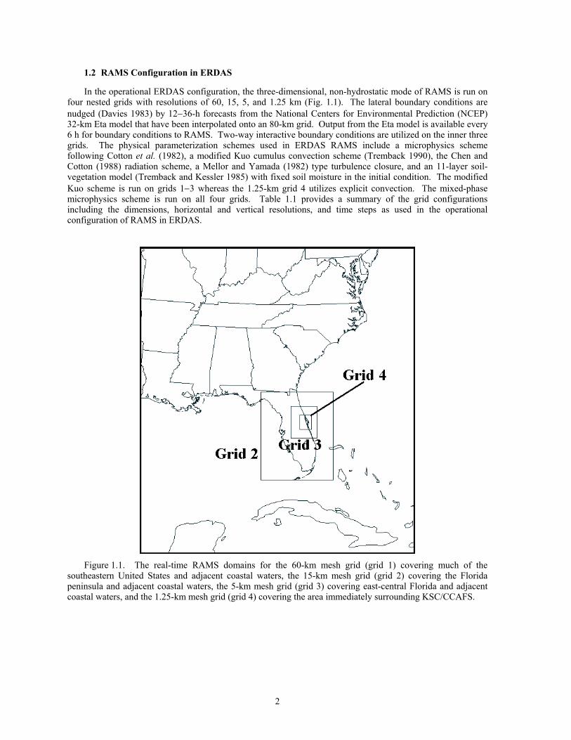
In the operational ERDAS configuration, the three-dimensional, non-hydrostatic mode of RAMS is run on four nested grids with resolutions of 60, 15, 5, and 1.25 km (Fig. 1.1). The lateral boundary conditions are nudged (Davies 1983) by 12−36-h forecasts from the National Centers for Environmental Prediction (NCEP) 32-km Eta model that have been interpolated onto an 80-km grid. Output from the Eta model is available every 6 h for boundary conditions to RAMS. Two-way interactive boundary conditions are utilized on the inner three grids. The physical parameterization schemes used in ERDAS RAMS include a microphysics scheme following Cotton et al. (1982), a modified Kuo cumulus convection scheme (Tremback 1990), the Chen and Cotton (1988) radiation scheme, a Mellor and Yamada (1982) type turbulence closure, and an 11-layer soil-vegetation model (Tremback and Kessler 1985) with fixed soil moisture in the initial condition. The modified Kuo scheme is run on grids 1−3 whereas the 1.25-km grid 4 utilizes explicit convection. The mixed-phase microphysics scheme is run on all four grids. Table 1.1 provides a summary of the grid configurations including the dimensions, horizontal and vertical resolutions, and time steps as used in the operational configuration of RAMS in ERDAS.

Figure 1.1. The real-time RAMS domains for the 60-km mesh grid (grid 1) covering much of the

southeastern United States and adjacent coastal waters, the 15-km mesh grid (grid 2) covering the Florida peninsula and adjacent coastal waters, the 5-km mesh grid (grid 3) covering east-central Florida and adjacent coastal waters, and the 1.25-km mesh grid (grid 4) covering the area immediately surrounding KSC/CCAFS.

3

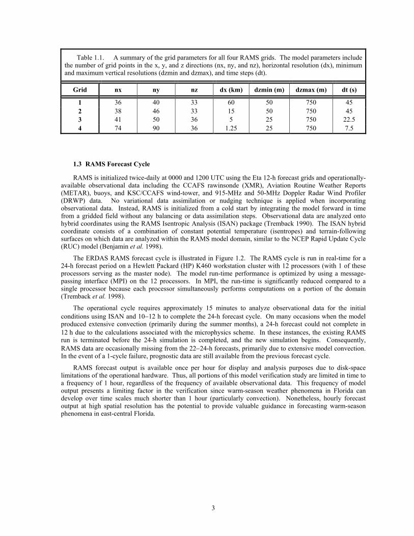
Table 1.1. A summary of the grid parameters for all four RAMS grids. The model parameters include the number of grid points in the x, y, and z directions (nx, ny, and nz), horizontal resolution (dx), minimum and maximum vertical resolutions (dzmin and dzmax), and time steps (dt).

Grid nx ny nz dx (km) dzmin (m) dzmax (m) dt (s)

1 36 40 33 60 50 750 45 2 38 46 33 15 50 750 45 3 41 50 36 5 25 750 22.5 4 74 90 36 1.25 25 750 7.5

1.3 RAMS Forecast Cycle

RAMS is initialized twice-daily at 0000 and 1200 UTC using the Eta 12-h forecast grids and operationally-available observational data including the CCAFS rawinsonde (XMR), Aviation Routine Weather Reports (METAR), buoys, and KSC/CCAFS wind-tower, and 915-MHz and 50-MHz Doppler Radar Wind Profiler (DRWP) data. No variational data assimilation or nudging technique is applied when incorporating observational data. Instead, RAMS is initialized from a cold start by integrating the model forward in time from a gridded field without any balancing or data assimilation steps. Observational data are analyzed onto hybrid coordinates using the RAMS Isentropic Analysis (ISAN) package (Tremback 1990). The ISAN hybrid coordinate consists of a combination of constant potential temperature (isentropes) and terrain-following surfaces on which data are analyzed within the RAMS model domain, similar to the NCEP Rapid Update Cycle (RUC) model (Benjamin et al. 1998).

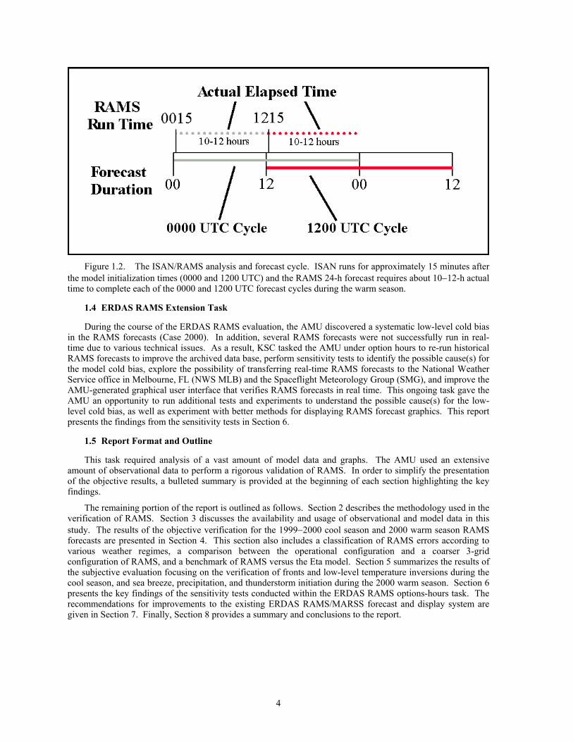
The ERDAS RAMS forecast cycle is illustrated in Figure 1.2. The RAMS cycle is run in real-time for a 24-h forecast period on a Hewlett Packard (HP) K460 workstation cluster with 12 processors (with 1 of these processors serving as the master node). The model run-time performance is optimized by using a message-passing interface (MPI) on the 12 processors. In MPI, the run-time is significantly reduced compared to a single processor because each processor simultaneously performs computations on a portion of the domain (Tremback et al. 1998).

The operational cycle requires approximately 15 minutes to analyze observational data for the initial conditions using ISAN and 10−12 h to complete the 24-h forecast cycle. On many occasions when the model produced extensive convection (primarily during the summer months), a 24-h forecast could not complete in 12 h due to the calculations associated with the microphysics scheme. In these instances, the existing RAMS run is terminated before the 24-h simulation is completed, and the new simulation begins. Consequently, RAMS data are occasionally missing from the 22−24-h forecasts, primarily due to extensive model convection. In the event of a 1-cycle failure, prognostic data are still available from the previous forecast cycle.

RAMS forecast output is available once per hour for display and analysis purposes due to disk-space limitations of the operational hardware. Thus, all portions of this model verification study are limited in time to a frequency of 1 hour, regardless of the frequency of available observational data. This frequency of model output presents a limiting factor in the verification since warm-season weather phenomena in Florida can develop over time scales much shorter than 1 hour (particularly convection). Nonetheless, hourly forecast output at high spatial resolution has the potential to provide valuable guidance in forecasting warm-season phenomena in east-central Florida.

4

Figure 1.2. The ISAN/RAMS analysis and forecast cycle. ISAN runs for approximately 15 minutes after

the model initialization times (0000 and 1200 UTC) and the RAMS 24-h forecast requires about 10−12-h actual time to complete each of the 0000 and 1200 UTC forecast cycles during the warm season.

1.4 ERDAS RAMS Extension Task

During the course of the ERDAS RAMS evaluation, the AMU discovered a systematic low-level cold bias in the RAMS forecasts (Case 2000). In addition, several RAMS forecasts were not successfully run in real-time due to various technical issues. As a result, KSC tasked the AMU under option hours to re-run historical RAMS forecasts to improve the archived data base, perform sensitivity tests to identify the possible cause(s) for the model cold bias, explore the possibility of transferring real-time RAMS forecasts to the National Weather Service office in Melbourne, FL (NWS MLB) and the Spaceflight Meteorology Group (SMG), and improve the AMU-generated graphical user interface that verifies RAMS forecasts in real time. This ongoing task gave the AMU an opportunity to run additional tests and experiments to understand the possible cause(s) for the low-level cold bias, as well as experiment with better methods for displaying RAMS forecast graphics. This report presents the findings from the sensitivity tests in Section 6.

1.5 Report Format and Outline

This task required analysis of a vast amount of model data and graphs. The AMU used an extensive amount of observational data to perform a rigorous validation of RAMS. In order to simplify the presentation of the objective results, a bulleted summary is provided at the beginning of each section highlighting the key findings.

The remaining portion of the report is outlined as follows. Section 2 describes the methodology used in the verification of RAMS. Section 3 discusses the availability and usage of observational and model data in this study. The results of the objective verification for the 1999−2000 cool season and 2000 warm season RAMS forecasts are presented in Section 4. This section also includes a classification of RAMS errors according to various weather regimes, a comparison between the operational configuration and a coarser 3-grid configuration of RAMS, and a benchmark of RAMS versus the Eta model. Section 5 summarizes the results of the subjective evaluation focusing on the verification of fronts and low-level temperature inversions during the cool season, and sea breeze, precipitation, and thunderstorm initiation during the 2000 warm season. Section 6 presents the key findings of the sensitivity tests conducted within the ERDAS RAMS options-hours task. The recommendations for improvements to the existing ERDAS RAMS/MARSS forecast and display system are given in Section 7. Finally, Section 8 provides a summary and conclusions to the report.

5

2. Methodology

The AMU evaluation of RAMS during the 1999−2000 cool, and 1999 and 2000 warm seasons includes both an objective and subjective component, following the methodology used in the interim ERDAS RAMS report. The objective component is designed to present a representative set of model errors of winds, temperature, and moisture for both the surface and upper-levels. The goal of the subjective verification is to provide an assessment of the forecast timing and propagation of the east-central Florida East Coast Sea Breeze (ECSB), daytime forecast precipitation, and forecast thunderstorm initiation by examining selected RAMS forecast fields. Since the 1999 warm-season objective and subjective results were thoroughly discussed in the interim report, this final report will focus on results from the 1999-2000 cool and 2000 warm seasons.

2.1 Objective Component

The objective component of the RAMS evaluation consists of five separate segments listed below that compute point error statistics:

• Verification of the operational 4-grid configuration of RAMS.

• Surface wind regime classification.

• Thunderstorm day regime classification.

• Comparison of point error statistics between the operational configuration and a RAMS configuration with a coarser horizontal resolution

• Comparison of RAMS errors to the Eta model errors.

Each portion of the objective component focuses on point error statistics at many different observational locations on all four forecast grids with emphasis placed on stations in grid 4.

2.1.1 Standard Evaluation

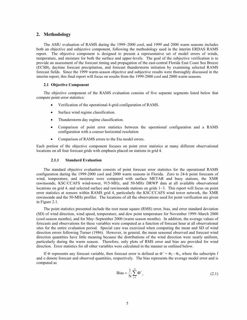
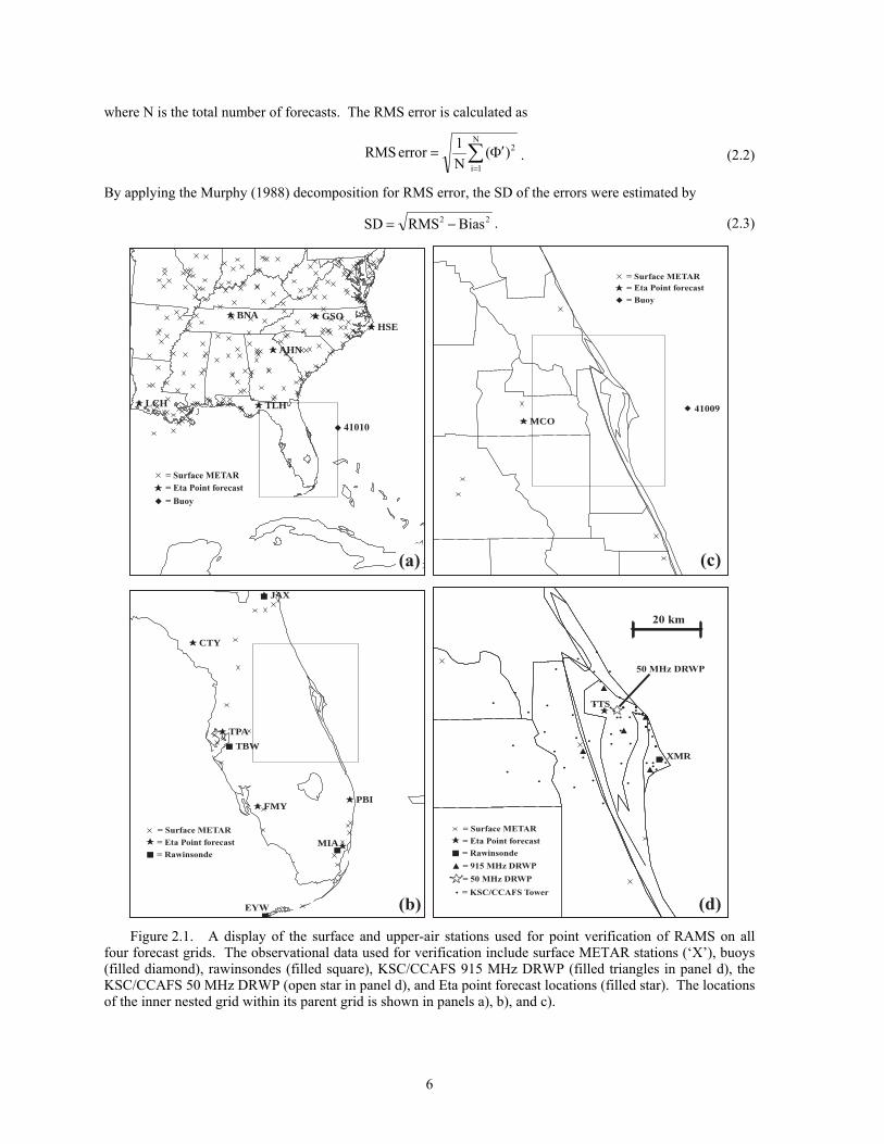
The standard objective evaluation consists of point forecast error statistics for the operational RAMS configuration during the 1999-2000 cool and 2000 warm seasons in Florida. Zero to 24-h point forecasts of wind, temperature, and moisture were compared with surface METAR and buoy stations, the XMR rawinsonde, KSC/CCAFS wind-tower, 915-MHz, and 50-MHz DRWP data at all available observational locations on grid 4, and selected surface and rawinsonde stations on grids 1−3. This report will focus on point error statistics at sensors within RAMS grid 4, particularly the KSC/CCAFS wind tower network, the XMR rawinsonde and the 50-MHz profiler. The locations of all the observations used for point verification are given in Figure 2.1.

The point statistics presented include the root mean square (RMS) error, bias, and error standard deviation (SD) of wind direction, wind speed, temperature, and dew point temperature for November 1999−March 2000 (cool-season months), and for May−September 2000 (warm season months). In addition, the average values of forecasts and observations for these variables were computed as a function of forecast hour at all observational sites for the entire evaluation period. Special care was exercised when computing the mean and SD of wind direction errors following Turner (1986). However, in general, the mean seasonal observed and forecast wind direction quantities have little meaning because the distributions of the wind direction were nearly uniform, particularly during the warm season. Therefore, only plots of RMS error and bias are provided for wind direction. Error statistics for all other variables were calculated in the manner as outlined below.

If Φ represents any forecast variable, then forecast error is defined as Φ’ = Φf - Φo, where the subscripts f and o denote forecast and observed quantities, respectively. The bias represents the average model error and is computed as

∑=

Φ′=N

1iN1Bias , (2.1)

6

where N is the total number of forecasts. The RMS error is calculated as

2N

1i)(

N1error RMS ∑

=

Φ′= . (2.2)

By applying the Murphy (1988) decomposition for RMS error, the SD of the errors were estimated by

22 BiasRMSSD −= . (2.3)

AHN

BNA GSOHSE

TLHLCH

41010

(a)

= Surface METAR= Eta Point forecast

= Buoy

MCO

(c)

41009

= Surface METAR= Eta Point forecast

= Buoy

CTY

FMY

JAX

MIA

PBI

TPA

TBW

(b)EYW

= Surface METAR

= Eta Point forecast

= Rawinsonde

TTS

XMR

50 MHz DRWP

(d)

= Surface METAR

= Eta Point forecast

= Rawinsonde

= 915 MHz DRWP

= 50 MHz DRWP

= KSC/CCAFS Tower

20 km

Figure 2.1. A display of the surface and upper-air stations used for point verification of RAMS on all

four forecast grids. The observational data used for verification include surface METAR stations (‘X’), buoys (filled diamond), rawinsondes (filled square), KSC/CCAFS 915 MHz DRWP (filled triangles in panel d), the KSC/CCAFS 50 MHz DRWP (open star in panel d), and Eta point forecast locations (filled star). The locations of the inner nested grid within its parent grid is shown in panels a), b), and c).

7

For purposes of interpretation in this report, we have assumed that the magnitude of the observational error is negligible compared to the model error. The total model error (RMS error) includes contributions from both systematic and random errors. Systematic error (bias) can be caused by a consistent misrepresentation of physical parameters such as radiation or model-generated convection. Random or nonsystematic errors, given by the error SD, represent the errors caused by uncertainties in the model initial condition or unresolveable differences in scales between the forecasts and observations. Note that the error standard deviation contains a component of natural variability since the model value is an average over a grid volume whereas the observed value is usually a point measurement.

A quality control (QC) check was performed on all point error statistics to remove any errors greater than 3 standard deviations from the mean error (bias). This QC check was performed to screen out bad observations or corrupted model forecasts and generally resulted in the rejection of less than 2 percent of all possible errors.

2.1.2 Regime Classifications

The second and third segments of the objective evaluation involve the computation of point error statistics under various weather regimes for the operational RAMS configuration during the 2000 warm season. Specifically, two types of regimes are examined in this report, surface winds and thunderstorm days. During each day, the surface wind regime was identified according to the early morning wind flow observed across the KSC/CCAFS wind-tower network. The days were then grouped into three classes of wind-flow patterns: westerly (offshore), easterly (onshore), and light or light and variable, where light wind regimes were defined as sustained speeds less than 5 knots. The RAMS forecasts were grouped together according to the similar surface wind regimes and error statistics were compiled for the similar wind regimes.

For the thunderstorm regime classification, the RAMS point forecasts were computed for all combinations of forecast and observed thunderstorms on grid 4. Every day was categorized according to the occurrence of observed or forecast thunderstorms within the area of the RAMS grid 4. Each RAMS forecast fell into one of four categories: both observed and forecast thunderstorms, observed but no forecast thunderstorms, forecast but no observed thunderstorms, and no observed or forecast thunderstorms. Point error statistics were computed for each of these four combinations of thunderstorm days during the 2000 warm season. The results of the regime classification experiments are presented in Section 5.2.3.

2.1.3 Benchmark Experiments

The fourth and fifth segments of the objective evaluation consist of two benchmark experiments. One benchmark experiment compares the RAMS 4-grid operational configuration to a 3-grid configuration by simply excluding grid 4 and rerunning RAMS with only grids 1, 2, and 3. The statistics were computed separately for the 3-grid and 4-grid data for the forecast cycles when both models runs were available (refer to Appendix A). Section 4.5 presents the results of this comparison for observational data within the grid 4 domain. The goal of this experiment is to measure the impact from a decrease in horizontal resolution of the innermost grid on the resulting forecast errors.

The second benchmark experiment compares the Eta point forecasts at 14 surface stations in the southeastern United States and 4 upper-air stations in the Florida peninsula to RAMS forecasts interpolated to the same stations (refer to Fig. 2.1 and Table 2.1). This important benchmark compares RAMS forecasts to the widely-used NCEP Eta model and quantifies any added value that may be provided by the RAMS over the Eta model, based on an objective comparison. This report will focus on the RAMS/Eta comparison at TTS (surface only), since this station is the only available location on RAMS grid 4. The results from the Eta model benchmark are discussed in Section 4.6.

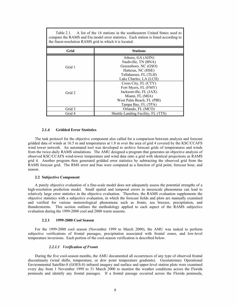
8

Table 2.1. A list of the 14 stations in the southeastern United States used to compare the RAMS and Eta model error statistics. Each station is listed according to the finest-resolution RAMS grid in which it is located.

Grid Stations

Grid 1

Athens, GA (AHN) Nashville, TN (BNA)

Greensboro, NC (GSO) Hatteras, NC (HSE)

Tallahassee, FL (TLH) Lake Charles, LA (LCH)

Grid 2

Cross City, FL (CTY) Fort Myers, FL (FMY) Jacksonville, FL (JAX)

Miami, FL (MIA) West Palm Beach, FL (PBI)

Tampa Bay, FL (TPA) Grid 3 Orlando, FL (MCO) Grid 4 Shuttle Landing Facility, FL (TTS)

2.1.4 Gridded Error Statistics

The task protocol for the objective component also called for a comparison between analysis and forecast gridded data of winds at 16.5 m and temperatures at 1.8 m over the area of grid 4 covered by the KSC/CCAFS wind tower network. An automated tool was developed to archive forecast grids of temperatures and winds from the twice-daily RAMS simulations. The AMU designed a program that generates an objective analysis of observed KSC/CCAFS wind-tower temperature and wind data onto a grid with identical projections as RAMS grid 4. Another program then generated gridded error statistics by subtracting the observed grid from the RAMS forecast grid. The RMS error and bias were computed as a function of grid point, forecast hour, and season.

2.2 Subjective Component

A purely objective evaluation of a fine-scale model does not adequately assess the potential strengths of a high-resolution prediction model. Small spatial and temporal errors in mesoscale phenomena can lead to relatively large error statistics in the objective evaluation. Therefore, the RAMS evaluation supplements the objective statistics with a subjective evaluation, in which the forecast fields and plots are manually examined and verified for various meteorological phenomena such as fronts, sea breezes, precipitation, and thunderstorms. This section outlines the methodology applied to each aspect of the RAMS subjective evaluation during the 1999-2000 cool and 2000 warm seasons.

2.2.1 1999-2000 Cool Season

For the 1999-2000 cool season (November 1999 to March 2000), the AMU was tasked to perform subjective verifications of frontal passages, precipitation associated with frontal zones, and low-level temperature inversions. Each portion of the cool-season verification is described below.

2.2.1.1 Verification of Fronts

During the five cool-season months, the AMU documented all occurrences of any type of observed frontal discontinuity (wind shifts, temperature, or dew point temperature gradients). Geostationary Operational Environmental Satellite-8 (GOES-8) infrared imagery and surface and upper-level station plots were examined every day from 1 November 1999 to 31 March 2000 to monitor the weather conditions across the Florida peninsula and identify any frontal passages. If a frontal passage occurred across the Florida peninsula,

9

graphical traces (meteograms) of hourly temperature, dew point temperature, wind direction, wind speed, and mean sea-level pressure observations and RAMS forecasts were examined at seven selected surface stations on the east coast of the Florida peninsula (Jacksonville (JAX), Daytona Beach (DAB), the Shuttle Landing Facility (TTS), Melbourne (MLB), Vero Beach (VRB), West Palm Beach (PBI), and Miami (MIA)). Frontal passages were verified for both the 0000 UTC and 1200 UTC RAMS forecast cycles whenever the 24-h forecast overlapped an observed frontal passage and sufficient archived forecast and observed data were available. The discontinuities in winds, temperature, and dew point temperature were each verified independently because the wind shifts and temperature/dew point temperature gradients often occurred at different times with a frontal passage.

The forecast errors associated with frontal passages were examined for three criteria: pre-frontal conditions, the frontal transition zone, and post-frontal maximum wind speed. The pre-frontal forecast wind direction, temperature, and dew point temperature errors were obtained by differencing the observations from the RAMS forecast values at each surface station that experienced both a forecast and observed frontal passage. The errors in forecast frontal timing were computed to the nearest hour, limited by the frequency of available RAMS output. The intensity of the frontal zone was verified by comparing the observed and forecast 3-h changes in each meteorological quantity following the initial observed or forecast discontinuity. Finally, the maximum forecast post-frontal wind speed was verified against the maximum observed post-frontal wind speed for each forecast that experienced a frontal passage. The results of the frontal verification are presented in Section 5.1.1.

2.2.1.2 Verification of Precipitation

The 1999-2000 cool season offered only a small number of cases for frontal-associated precipitation verification. Very few significant frontal passages occurred with substantial frontal or pre-frontal rain bands, thereby preventing a robust verification of RAMS forecast precipitation during the cool season. The two most significant frontal events with precipitation across the Florida peninsula occurred on 2 November 1999 and 24 January 2000, but each case had problems in the RAMS forecast. The 0000 UTC RAMS forecast cycle failed on 2 November. On the 24 January case, the NCEP Eta model poorly predicted the development of an Atlantic coastal cyclone prediction, and thus did not provide adequate boundary conditions for the RAMS forecasts. Additional cases with weak or broken squall lines occurred on a few days in March.

Section 5.1.2 summarizes the most significant precipitation events for which sufficient forecast and observational data were available for subjective verification. In addition, a few RAMS forecasts are compared to observed satellite and rain-gauge data for the 24 January and 11 March 2000 events. To compare rain-gauge data to RAMS forecast precipitation, archived rainfall data from the St. John River, south Florida, and KSC networks were obtained from the Goddard Space Flight Center. An objective analysis was performed on the accumulated hourly rain-gauge data at every hour for the entire 1999-2000 cool season to obtain observed rainfall on RAMS grids 2, 3, and 4. RAMS forecast rainfall was then compared to these gridded rain-gauge data overlaid on infrared satellite imagery, primarily focusing on grid-2 for peninsula-scale rainfall verification associated with fronts and troughs.

2.2.1.3 Verification of Low-level Temperature Inversions

For all five cool-season months, the occurrence of observed and forecast temperature inversions at XMR were recorded in the lowest 3 km of the atmosphere, including both surface-based radiational inversions and elevated subsidence inversions. Approximately 80% of the cases examined were surface-based radiational inversions. Both the 0000 UTC and 1200 UTC RAMS forecast cycles were examined and verified against the observed morning XMR sounding, which was typically released at 1115 UTC. Therefore, the 11-h forecast from the 0000 UTC RAMS cycle and the 23-h forecast from the previous day’s 1200 UTC RAMS cycle are the verifying forecast hours.

The number of model forecast “hits” and “misses” were compiled to determine how well RAMS can predict the occurrence of a temperature inversion. When both an observed and forecast inversion occurred, specific parameters were verified including the intensity of the temperature inversion in °C, the height of the inversion base in meters, and the depth of the inversion layer in meters.

10

2.2.2 1999 and 2000 Warm Seasons

To supplement the 1999 warm-season results from the ERDAS RAMS interim report, the AMU was tasked to perform an additional sea-breeze and precipitation verification, as well as a thunderstorm initiation verification for the 2000 warm season. The comprehensive sea-breeze verification in this report contains results for both 1999 and 2000, whereas the precipitation and thunderstorm initiation verification results are only for the 2000 warm season. The methodology for each of these three studies is described below.

2.2.2.1 Verification of Sea breeze for the 1999 and 2000 Warm Seasons

As in the ERDAS RAMS interim report, the AMU conducted a sea-breeze verification at several individual KSC/CCAFS wind towers located over east-central Florida (Case 2000). For this final report, the AMU fine-tuned the verification methodology used in the interim report to increase the size of the data base, facilitate the efficiency of the verification technique, and increase the stringency of the original sea-breeze evaluation. To increase the sample size, the AMU examined all archived RAMS forecasts for 1999 and 2000 rather than AMU working days only. Note that the 2000 warm season includes forecasts from May−September whereas the 1999 warm season only includes forecasts from May−August due to non-availability of Eta background grids and boundary conditions during much of September 1999. The archived point forecasts and observations were converted to the General Meteorological Package (GEMPAK) format for analysis and display at all available wind towers.

To facilitate the efficiency of the verification technique, the AMU selected 12 rather than 13 wind towers to conduct the modified ECSB verification, representing 3 different zones in the network (the coastal barrier islands, Merritt Island, and mainland Florida). In each zone, 4 towers were identified in a north-south orientation that contained the most data for both the 1999 and 2000 Florida warm seasons. Twelve-panel graphical plots (meteograms) displaying both the forecast and observed wind direction and speed were generated for all RAMS forecast cycles to verify the occurrence and timing of the ECSB at all selected towers. Where possible, the same towers were used in the modified verification as in the interim report study; however, during the 2000 warm season, several KSC/CCAFS wind towers experienced significant data outages due to Range Standardization and Automation (RSA) testing. The wind towers with the most missing data were those well west of the Indian river over mainland Florida. Thus, only towers near the Indian river could be used to represent the mainland Florida zone.

The AMU utilized both GOES-8 visible imagery and Weather Surveillance Radar, model 74C (WSR-74C) reflectivity data to identify the occurrence of the ECSB. An observed sea breeze is typically accompanied by a sharp clearing line and reflectivity fine line, which propagate westward with the sea breeze. To determine the occurrence and timing of the sea-breeze passage, the AMU examined each KSC/CCAFS tower for a development or wind-shift to an onshore wind component (wind direction between 335° and 155°, the approximate orientation of the Florida coastline). During easterly flow regimes, a sea-breeze passage was determined by a distinct increase in the negative (easterly) u-wind at each KSC/CCAFS tower. The AMU then applied these same wind criteria to the ERDAS RAMS forecasts interpolated to each KSC/CCAFS tower location to determine the forecast ECSB passage.

To increase the stringency of the evaluation, the occurrence of a forecast sea breeze was verified on a per-tower basis at each selected tower rather than at any tower (as was done in the interim report). This modified methodology not only demands more accuracy in the model predictions, but it also increases the size of the data base. Finally, the stringency of the analysis was also increased by refining the definition of an onshore versus offshore wind at coastal towers 1 and 3. At these towers, the wind directions representing onshore flow were expanded due to the specific orientation of the coastline along the Cape (Fig. 2.2). Onshore flow was defined as a wind direction between 180° and 335° at tower 1 and between 200° and 335° at tower 3. As a result, both of these towers have a larger range of wind directions that are onshore compared to the other selected towers.

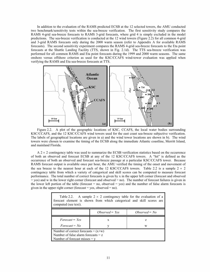
11

In addition to the evaluation of the RAMS predicted ECSB at the 12 selected towers, the AMU conducted two benchmark/sensitivity tests within the sea-breeze verification. The first sensitivity study compares the RAMS 4-grid sea-breeze forecasts to RAMS 3-grid forecasts, where grid 4 is simply excluded in the model predictions. The sea-breeze verification is conducted at the 12 wind towers (Figure 2.2) for all common 4-grid and 3-grid RAMS forecasts only during the 2000 warm season (refer to Appendix A for available RAMS forecasts). The second sensitivity experiment compares the RAMS 4-grid sea-breeze forecasts to the Eta point forecasts at the Shuttle Landing Facility (TTS, shown in Fig. 2.1d). The TTS sea-breeze verification was performed for all common RAMS and Eta point forecasts during the 1999 and 2000 warm seasons. The same onshore versus offshore criterion as used for the KSC/CCAFS wind-tower evaluation was applied when verifying the RAMS and Eta sea-breeze forecasts at TTS.

Figure 2.2. A plot of the geographic locations of KSC, CCAFS, the local water bodies surrounding

KSC/CCAFS, and the 12 KSC/CCAFS wind towers used for the east coast sea-breeze subjective verification. The labels of geographical locations are given in a) and the wind tower locations are shown in b). The wind towers were chosen to examine the timing of the ECSB along the immediate Atlantic coastline, Merritt Island, and mainland Florida.

A 2 × 2 contingency table was used to summarize the ECSB verification statistics based on the occurrence of both an observed and forecast ECSB at any of the 12 KSC/CCAFS towers. A “hit” is defined as the occurrence of both an observed and forecast sea-breeze passage at a particular KSC/CCAFS tower. Because RAMS forecast output is available once per hour, the AMU verified the timing of the onset and movement of the sea breeze to the nearest hour at each of the 12 KSC/CCAFS towers. Table 2.2 is a sample 2 × 2 contingency table from which a variety of categorical and skill scores can be computed to measure forecast performance. The total number of correct forecasts is given by x in the upper left corner (forecast and observed = yes) and w in the lower right corner (forecast and observed = no). The number of forecast failures is given in the lower left portion of the table (forecast = no, observed = yes) and the number of false alarm forecasts is given in the upper right corner (forecast = yes, observed = no).

Table 2.2. A sample 2 × 2 contingency table for the evaluation of a forecast element is shown from which categorical and skill scores are computed (see text).

Observed = Yes Observed = No

Forecast = Yes x z

Forecast = No y w Number of correct forecasts = (x+w) Number of false alarm forecasts = z Number of forecast misses = y

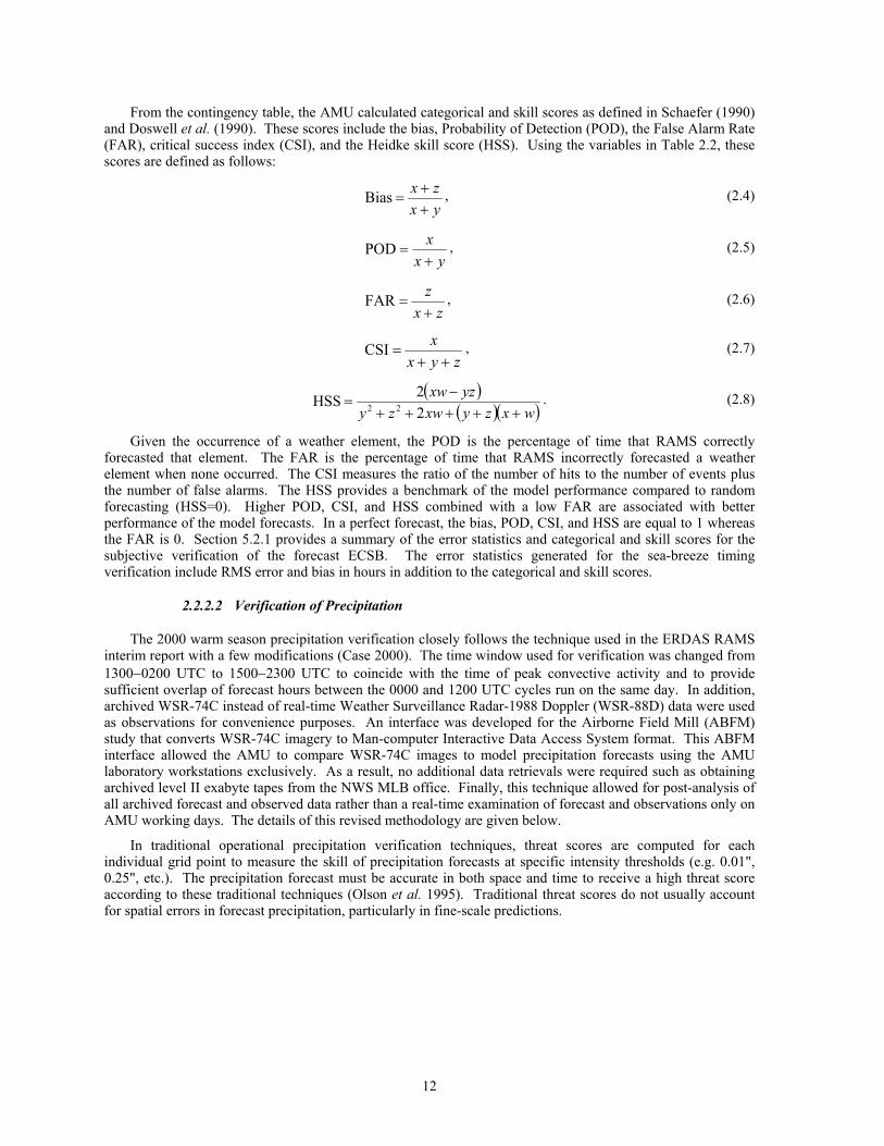
12

From the contingency table, the AMU calculated categorical and skill scores as defined in Schaefer (1990) and Doswell et al. (1990). These scores include the bias, Probability of Detection (POD), the False Alarm Rate (FAR), critical success index (CSI), and the Heidke skill score (HSS). Using the variables in Table 2.2, these scores are defined as follows:

yxzx

++

=Bias , (2.4)

yxx+

=POD , (2.5)

zxz+

=FAR , (2.6)

zyxx

++=CSI , (2.7)

( )( )( )wxzyxwzyyzxw

+++++−

=22HSS 22

. (2.8)

Given the occurrence of a weather element, the POD is the percentage of time that RAMS correctly forecasted that element. The FAR is the percentage of time that RAMS incorrectly forecasted a weather element when none occurred. The CSI measures the ratio of the number of hits to the number of events plus the number of false alarms. The HSS provides a benchmark of the model performance compared to random forecasting (HSS=0). Higher POD, CSI, and HSS combined with a low FAR are associated with better performance of the model forecasts. In a perfect forecast, the bias, POD, CSI, and HSS are equal to 1 whereas the FAR is 0. Section 5.2.1 provides a summary of the error statistics and categorical and skill scores for the subjective verification of the forecast ECSB. The error statistics generated for the sea-breeze timing verification include RMS error and bias in hours in addition to the categorical and skill scores.

2.2.2.2 Verification of Precipitation

The 2000 warm season precipitation verification closely follows the technique used in the ERDAS RAMS interim report with a few modifications (Case 2000). The time window used for verification was changed from 1300−0200 UTC to 1500−2300 UTC to coincide with the time of peak convective activity and to provide sufficient overlap of forecast hours between the 0000 and 1200 UTC cycles run on the same day. In addition, archived WSR-74C instead of real-time Weather Surveillance Radar-1988 Doppler (WSR-88D) data were used as observations for convenience purposes. An interface was developed for the Airborne Field Mill (ABFM) study that converts WSR-74C imagery to Man-computer Interactive Data Access System format. This ABFM interface allowed the AMU to compare WSR-74C images to model precipitation forecasts using the AMU laboratory workstations exclusively. As a result, no additional data retrievals were required such as obtaining archived level II exabyte tapes from the NWS MLB office. Finally, this technique allowed for post-analysis of all archived forecast and observed data rather than a real-time examination of forecast and observations only on AMU working days. The details of this revised methodology are given below.

In traditional operational precipitation verification techniques, threat scores are computed for each individual grid point to measure the skill of precipitation forecasts at specific intensity thresholds (e.g. 0.01", 0.25", etc.). The precipitation forecast must be accurate in both space and time to receive a high threat score according to these traditional techniques (Olson et al. 1995). Traditional threat scores do not usually account for spatial errors in forecast precipitation, particularly in fine-scale predictions.

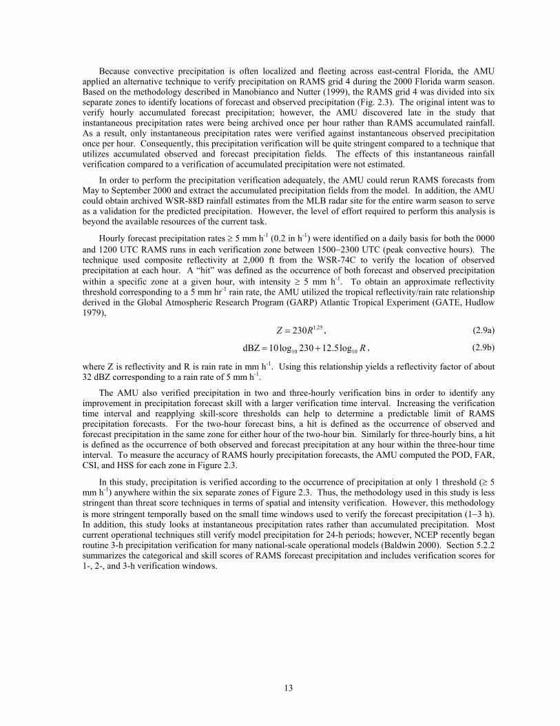
13

Because convective precipitation is often localized and fleeting across east-central Florida, the AMU applied an alternative technique to verify precipitation on RAMS grid 4 during the 2000 Florida warm season. Based on the methodology described in Manobianco and Nutter (1999), the RAMS grid 4 was divided into six separate zones to identify locations of forecast and observed precipitation (Fig. 2.3). The original intent was to verify hourly accumulated forecast precipitation; however, the AMU discovered late in the study that instantaneous precipitation rates were being archived once per hour rather than RAMS accumulated rainfall. As a result, only instantaneous precipitation rates were verified against instantaneous observed precipitation once per hour. Consequently, this precipitation verification will be quite stringent compared to a technique that utilizes accumulated observed and forecast precipitation fields. The effects of this instantaneous rainfall verification compared to a verification of accumulated precipitation were not estimated.

In order to perform the precipitation verification adequately, the AMU could rerun RAMS forecasts from May to September 2000 and extract the accumulated precipitation fields from the model. In addition, the AMU could obtain archived WSR-88D rainfall estimates from the MLB radar site for the entire warm season to serve as a validation for the predicted precipitation. However, the level of effort required to perform this analysis is beyond the available resources of the current task.

Hourly forecast precipitation rates ≥ 5 mm h-1 (0.2 in h-1) were identified on a daily basis for both the 0000 and 1200 UTC RAMS runs in each verification zone between 1500−2300 UTC (peak convective hours). The technique used composite reflectivity at 2,000 ft from the WSR-74C to verify the location of observed precipitation at each hour. A “hit” was defined as the occurrence of both forecast and observed precipitation within a specific zone at a given hour, with intensity ≥ 5 mm h-1. To obtain an approximate reflectivity threshold corresponding to a 5 mm hr-1 rain rate, the AMU utilized the tropical reflectivity/rain rate relationship derived in the Global Atmospheric Research Program (GARP) Atlantic Tropical Experiment (GATE, Hudlow 1979),

25.1230RZ = , (2.9a)

R1010 log5.12230log10dBZ += , (2.9b)

where Z is reflectivity and R is rain rate in mm h-1. Using this relationship yields a reflectivity factor of about 32 dBZ corresponding to a rain rate of 5 mm h-1.

The AMU also verified precipitation in two and three-hourly verification bins in order to identify any improvement in precipitation forecast skill with a larger verification time interval. Increasing the verification time interval and reapplying skill-score thresholds can help to determine a predictable limit of RAMS precipitation forecasts. For the two-hour forecast bins, a hit is defined as the occurrence of observed and forecast precipitation in the same zone for either hour of the two-hour bin. Similarly for three-hourly bins, a hit is defined as the occurrence of both observed and forecast precipitation at any hour within the three-hour time interval. To measure the accuracy of RAMS hourly precipitation forecasts, the AMU computed the POD, FAR, CSI, and HSS for each zone in Figure 2.3.

In this study, precipitation is verified according to the occurrence of precipitation at only 1 threshold (≥ 5 mm h-1) anywhere within the six separate zones of Figure 2.3. Thus, the methodology used in this study is less stringent than threat score techniques in terms of spatial and intensity verification. However, this methodology is more stringent temporally based on the small time windows used to verify the forecast precipitation (1−3 h). In addition, this study looks at instantaneous precipitation rates rather than accumulated precipitation. Most current operational techniques still verify model precipitation for 24-h periods; however, NCEP recently began routine 3-h precipitation verification for many national-scale operational models (Baldwin 2000). Section 5.2.2 summarizes the categorical and skill scores of RAMS forecast precipitation and includes verification scores for 1-, 2-, and 3-h verification windows.

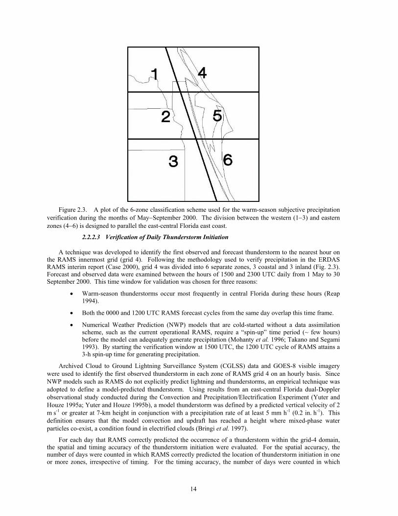
14

Figure 2.3. A plot of the 6-zone classification scheme used for the warm-season subjective precipitation

verification during the months of May−September 2000. The division between the western (1−3) and eastern zones (4−6) is designed to parallel the east-central Florida east coast.

2.2.2.3 Verification of Daily Thunderstorm Initiation

A technique was developed to identify the first observed and forecast thunderstorm to the nearest hour on the RAMS innermost grid (grid 4). Following the methodology used to verify precipitation in the ERDAS RAMS interim report (Case 2000), grid 4 was divided into 6 separate zones, 3 coastal and 3 inland (Fig. 2.3). Forecast and observed data were examined between the hours of 1500 and 2300 UTC daily from 1 May to 30 September 2000. This time window for validation was chosen for three reasons:

• Warm-season thunderstorms occur most frequently in central Florida during these hours (Reap 1994).

• Both the 0000 and 1200 UTC RAMS forecast cycles from the same day overlap this time frame.

• Numerical Weather Prediction (NWP) models that are cold-started without a data assimilation scheme, such as the current operational RAMS, require a “spin-up” time period (~ few hours) before the model can adequately generate precipitation (Mohanty et al. 1996; Takano and Segami 1993). By starting the verification window at 1500 UTC, the 1200 UTC cycle of RAMS attains a 3-h spin-up time for generating precipitation.

Archived Cloud to Ground Lightning Surveillance System (CGLSS) data and GOES-8 visible imagery were used to identify the first observed thunderstorm in each zone of RAMS grid 4 on an hourly basis. Since NWP models such as RAMS do not explicitly predict lightning and thunderstorms, an empirical technique was adopted to define a model-predicted thunderstorm. Using results from an east-central Florida dual-Doppler observational study conducted during the Convection and Precipitation/Electrification Experiment (Yuter and Houze 1995a; Yuter and Houze 1995b), a model thunderstorm was defined by a predicted vertical velocity of 2 m s-1 or greater at 7-km height in conjunction with a precipitation rate of at least 5 mm h-1 (0.2 in. h-1). This definition ensures that the model convection and updraft has reached a height where mixed-phase water particles co-exist, a condition found in electrified clouds (Bringi et al. 1997).

For each day that RAMS correctly predicted the occurrence of a thunderstorm within the grid-4 domain, the spatial and timing accuracy of the thunderstorm initiation were evaluated. For the spatial accuracy, the number of days were counted in which RAMS correctly predicted the location of thunderstorm initiation in one or more zones, irrespective of timing. For the timing accuracy, the number of days were counted in which

15

RAMS correctly predicted the initiation time exactly (0-h difference between observations and forecast), within 1 h (-1 to +1 h error), within 2 h (-2 to +2 h error), and within 3 h (-3 to +3 h error) of the observed time, irrespective of spatial accuracy. In addition, the spatial and timing accuracy of thunderstorm initiation were examined in combination by developing contingency tables and determining categorical and skill scores for each individual grid-4 zone based on specific timing thresholds. The results of the thunderstorm initiation verification are presented in Section 5.2.3.

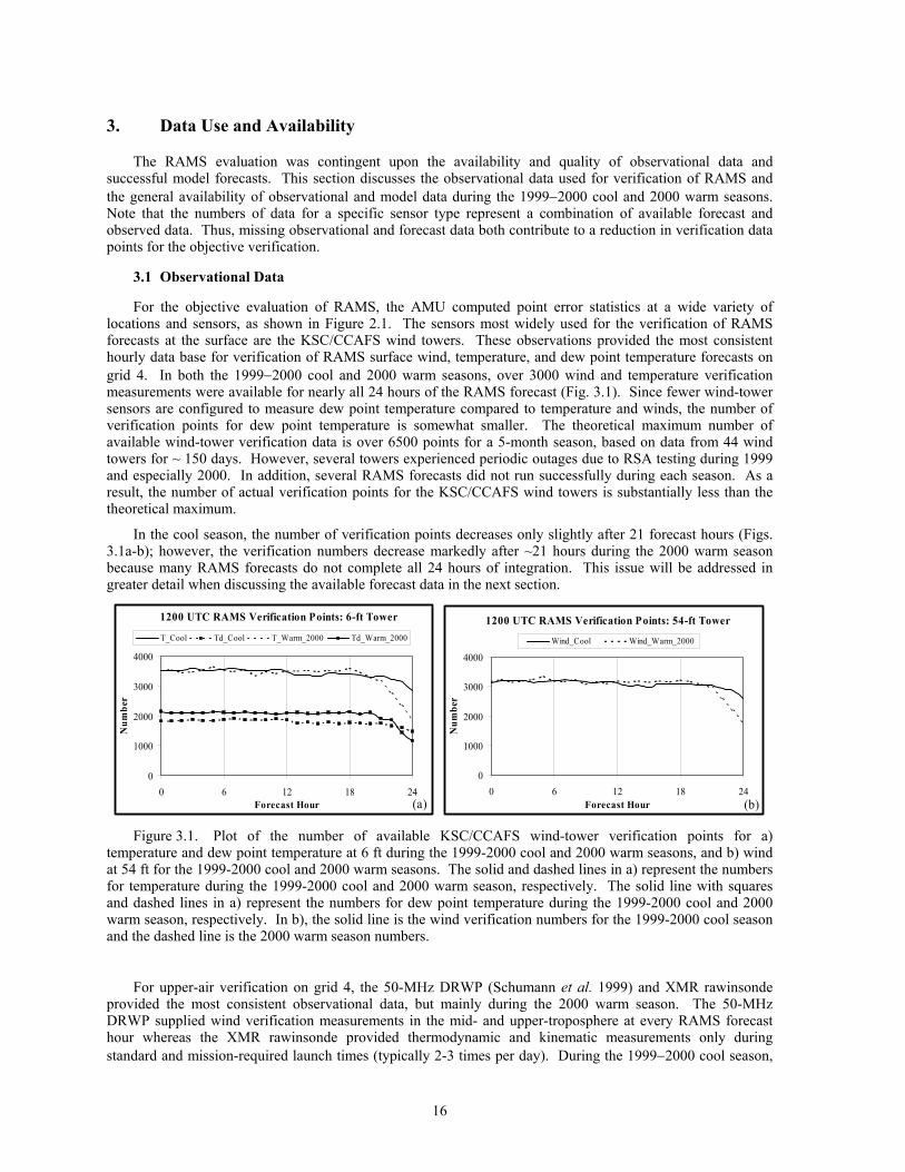
16

3. Data Use and Availability

The RAMS evaluation was contingent upon the availability and quality of observational data and successful model forecasts. This section discusses the observational data used for verification of RAMS and the general availability of observational and model data during the 1999−2000 cool and 2000 warm seasons. Note that the numbers of data for a specific sensor type represent a combination of available forecast and observed data. Thus, missing observational and forecast data both contribute to a reduction in verification data points for the objective verification.

3.1 Observational Data

For the objective evaluation of RAMS, the AMU computed point error statistics at a wide variety of locations and sensors, as shown in Figure 2.1. The sensors most widely used for the verification of RAMS forecasts at the surface are the KSC/CCAFS wind towers. These observations provided the most consistent hourly data base for verification of RAMS surface wind, temperature, and dew point temperature forecasts on grid 4. In both the 1999−2000 cool and 2000 warm seasons, over 3000 wind and temperature verification measurements were available for nearly all 24 hours of the RAMS forecast (Fig. 3.1). Since fewer wind-tower sensors are configured to measure dew point temperature compared to temperature and winds, the number of verification points for dew point temperature is somewhat smaller. The theoretical maximum number of available wind-tower verification data is over 6500 points for a 5-month season, based on data from 44 wind towers for ~ 150 days. However, several towers experienced periodic outages due to RSA testing during 1999 and especially 2000. In addition, several RAMS forecasts did not run successfully during each season. As a result, the number of actual verification points for the KSC/CCAFS wind towers is substantially less than the theoretical maximum.

In the cool season, the number of verification points decreases only slightly after 21 forecast hours (Figs. 3.1a-b); however, the verification numbers decrease markedly after ~21 hours during the 2000 warm season because many RAMS forecasts do not complete all 24 hours of integration. This issue will be addressed in greater detail when discussing the available forecast data in the next section.

1200 UTC RAMS Verification Points: 6-ft Tower

0

1000

2000

3000

4000

0 6 12 18 24Forecast Hour

Num

ber

T_Cool Td_Cool T_Warm_2000 Td_Warm_2000

(a)

1200 UTC RAMS Verification Points: 54-ft Tower

0

1000

2000

3000

4000

0 6 12 18 24Forecast Hour

Num

ber

Wind_Cool Wind_Warm_2000

(b) Figure 3.1. Plot of the number of available KSC/CCAFS wind-tower verification points for a)

temperature and dew point temperature at 6 ft during the 1999-2000 cool and 2000 warm seasons, and b) wind at 54 ft for the 1999-2000 cool and 2000 warm seasons. The solid and dashed lines in a) represent the numbers for temperature during the 1999-2000 cool and 2000 warm season, respectively. The solid line with squares and dashed lines in a) represent the numbers for dew point temperature during the 1999-2000 cool and 2000 warm season, respectively. In b), the solid line is the wind verification numbers for the 1999-2000 cool season and the dashed line is the 2000 warm season numbers.

For upper-air verification on grid 4, the 50-MHz DRWP (Schumann et al. 1999) and XMR rawinsonde provided the most consistent observational data, but mainly during the 2000 warm season. The 50-MHz DRWP supplied wind verification measurements in the mid- and upper-troposphere at every RAMS forecast hour whereas the XMR rawinsonde provided thermodynamic and kinematic measurements only during standard and mission-required launch times (typically 2-3 times per day). During the 1999−2000 cool season,

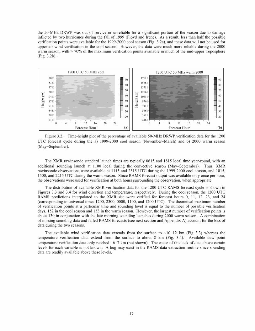
17

the 50-MHz DRWP was out of service or unreliable for a significant portion of the season due to damage inflicted by two hurricanes during the fall of 1999 (Floyd and Irene). As a result, less than half the possible verification points were available for the 1999-2000 cool season (Fig. 3.2a), and these data will not be used for upper-air wind verification in the cool season. However, the data were much more reliable during the 2000 warm season, with > 70% of the maximum verification points available in much of the mid-upper troposphere (Fig. 3.2b).

21613811546171118761

1041112061137111536117011

0 4 8 12 16 20 24

Forecast Hour

20

30

40

50

60

70

80

90

1200 UTC 50 MHz cool

(a)

21613811546171118761

1041112061137111536117011

0 4 8 12 16 20 24

Forecast Hour

20

30

40

50

60

70

80

90

1200 UTC 50 MHz warm 2000

(b) Figure 3.2. Time-height plot of the percentage of available 50-MHz DRWP verification data for the 1200

UTC forecast cycle during the a) 1999-2000 cool season (November−March) and b) 2000 warm season (May−September).

The XMR rawinsonde standard launch times are typically 0615 and 1815 local time year-round, with an additional sounding launch at 1100 local during the convective season (May−September). Thus, XMR rawinsonde observations were available at 1115 and 2315 UTC during the 1999-2000 cool season, and 1015, 1500, and 2215 UTC during the warm season. Since RAMS forecast output was available only once per hour, the observations were used for verification at both hours surrounding the observation, when appropriate.

The distribution of available XMR verification data for the 1200 UTC RAMS forecast cycle is shown in Figures 3.3 and 3.4 for wind direction and temperature, respectively. During the cool season, the 1200 UTC RAMS predictions interpolated to the XMR site were verified for forecast hours 0, 11, 12, 23, and 24 (corresponding to universal times 1200, 2300, 0000, 1100, and 1200 UTC). The theoretical maximum number of verification points at a particular time and sounding level is equal to the number of possible verification days, 152 in the cool season and 153 in the warm season. However, the largest number of verification points is about 130 in conjunction with the late-morning sounding launches during 2000 warm season. A combination of missing sounding data and failed RAMS forecasts (see next section and Appendix A) account for the loss of data during the two seasons.

The available wind verification data extends from the surface to ~10−12 km (Fig 3.3) whereas the temperature verification data extend from the surface to about 8 km (Fig. 3.4). Available dew point temperature verification data only reached ~6−7 km (not shown). The cause of this lack of data above certain levels for each variable is not known. A bug may exist in the RAMS data extraction routine since sounding data are readily available above these levels.

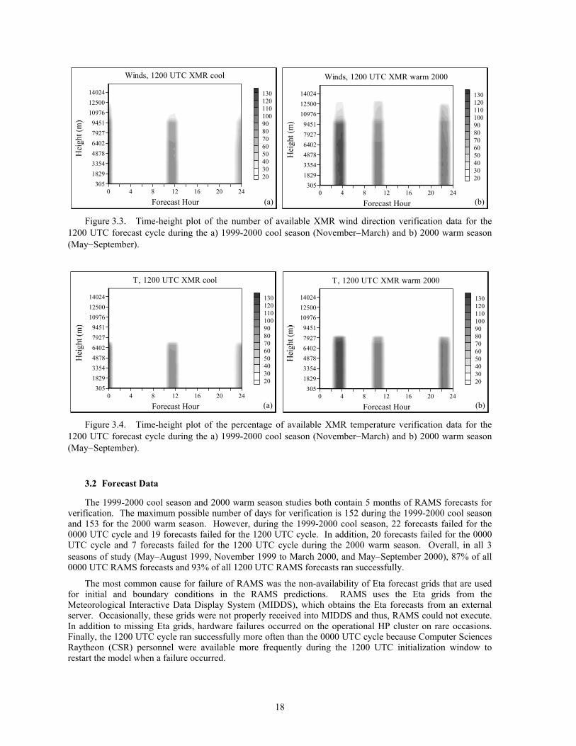
18

305182933544878640279279451

109761250014024

0 4 8 12 16 20 24

Forecast Hour

2030405060708090100110120130

Winds, 1200 UTC XMR cool

(a)

305182933544878640279279451

109761250014024

0 4 8 12 16 20 24

Forecast Hour

2030405060708090100110120130

Winds, 1200 UTC XMR warm 2000

(b) Figure 3.3. Time-height plot of the number of available XMR wind direction verification data for the

1200 UTC forecast cycle during the a) 1999-2000 cool season (November−March) and b) 2000 warm season (May−September).

305182933544878640279279451

109761250014024

0 4 8 12 16 20 24

Forecast Hour

2030405060708090100110120130

T, 1200 UTC XMR cool

(a)

305182933544878640279279451

109761250014024

0 4 8 12 16 20 24

Forecast Hour

2030405060708090100110120130

T, 1200 UTC XMR warm 2000

(b) Figure 3.4. Time-height plot of the percentage of available XMR temperature verification data for the

1200 UTC forecast cycle during the a) 1999-2000 cool season (November−March) and b) 2000 warm season (May−September).

3.2 Forecast Data

The 1999-2000 cool season and 2000 warm season studies both contain 5 months of RAMS forecasts for verification. The maximum possible number of days for verification is 152 during the 1999-2000 cool season and 153 for the 2000 warm season. However, during the 1999-2000 cool season, 22 forecasts failed for the 0000 UTC cycle and 19 forecasts failed for the 1200 UTC cycle. In addition, 20 forecasts failed for the 0000 UTC cycle and 7 forecasts failed for the 1200 UTC cycle during the 2000 warm season. Overall, in all 3 seasons of study (May−August 1999, November 1999 to March 2000, and May−September 2000), 87% of all 0000 UTC RAMS forecasts and 93% of all 1200 UTC RAMS forecasts ran successfully.

The most common cause for failure of RAMS was the non-availability of Eta forecast grids that are used for initial and boundary conditions in the RAMS predictions. RAMS uses the Eta grids from the Meteorological Interactive Data Display System (MIDDS), which obtains the Eta forecasts from an external server. Occasionally, these grids were not properly received into MIDDS and thus, RAMS could not execute. In addition to missing Eta grids, hardware failures occurred on the operational HP cluster on rare occasions. Finally, the 1200 UTC cycle ran successfully more often than the 0000 UTC cycle because Computer Sciences Raytheon (CSR) personnel were available more frequently during the 1200 UTC initialization window to restart the model when a failure occurred.

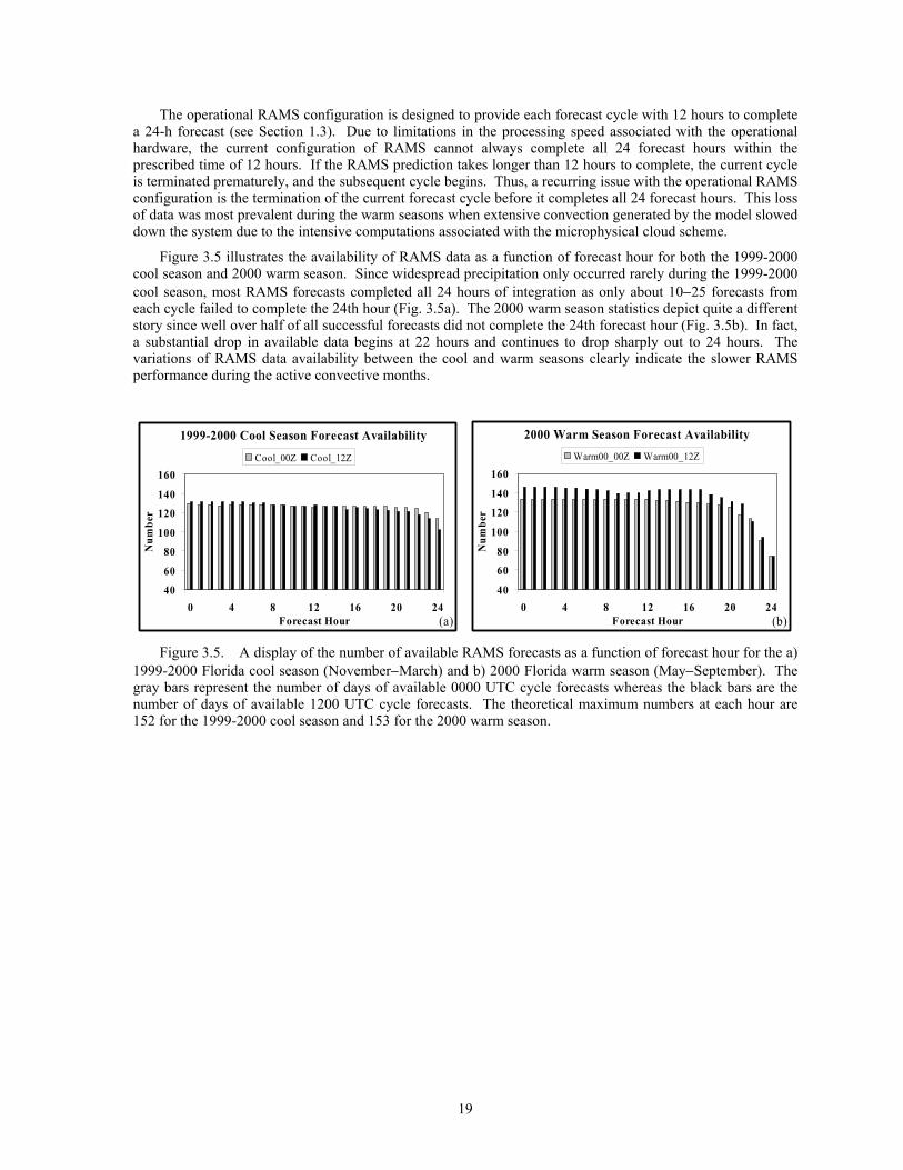
19

The operational RAMS configuration is designed to provide each forecast cycle with 12 hours to complete a 24-h forecast (see Section 1.3). Due to limitations in the processing speed associated with the operational hardware, the current configuration of RAMS cannot always complete all 24 forecast hours within the prescribed time of 12 hours. If the RAMS prediction takes longer than 12 hours to complete, the current cycle is terminated prematurely, and the subsequent cycle begins. Thus, a recurring issue with the operational RAMS configuration is the termination of the current forecast cycle before it completes all 24 forecast hours. This loss of data was most prevalent during the warm seasons when extensive convection generated by the model slowed down the system due to the intensive computations associated with the microphysical cloud scheme.

Figure 3.5 illustrates the availability of RAMS data as a function of forecast hour for both the 1999-2000 cool season and 2000 warm season. Since widespread precipitation only occurred rarely during the 1999-2000 cool season, most RAMS forecasts completed all 24 hours of integration as only about 10−25 forecasts from each cycle failed to complete the 24th hour (Fig. 3.5a). The 2000 warm season statistics depict quite a different story since well over half of all successful forecasts did not complete the 24th forecast hour (Fig. 3.5b). In fact, a substantial drop in available data begins at 22 hours and continues to drop sharply out to 24 hours. The variations of RAMS data availability between the cool and warm seasons clearly indicate the slower RAMS performance during the active convective months.

1999-2000 Cool Season Forecast Availability

40

60

80

100

120

140

160

0 4 8 12 16 20 24Forecast Hour

Num

ber

Cool_00Z Cool_12Z

(a)

2000 Warm Season Forecast Availability

40

60

80

100

120

140

160

0 4 8 12 16 20 24Forecast Hour

Num

ber

Warm00_00Z Warm00_12Z

(b) Figure 3.5. A display of the number of available RAMS forecasts as a function of forecast hour for the a)

1999-2000 Florida cool season (November−March) and b) 2000 Florida warm season (May−September). The gray bars represent the number of days of available 0000 UTC cycle forecasts whereas the black bars are the number of days of available 1200 UTC cycle forecasts. The theoretical maximum numbers at each hour are 152 for the 1999-2000 cool season and 153 for the 2000 warm season.

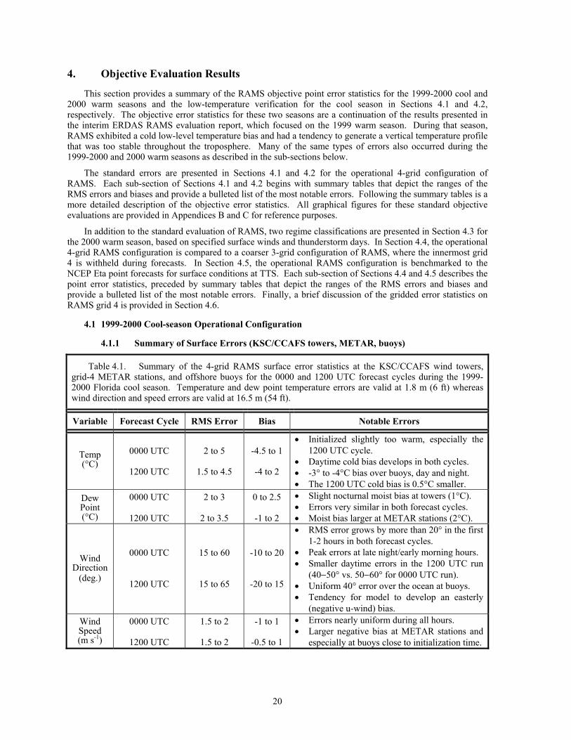
20

4. Objective Evaluation Results

This section provides a summary of the RAMS objective point error statistics for the 1999-2000 cool and 2000 warm seasons and the low-temperature verification for the cool season in Sections 4.1 and 4.2, respectively. The objective error statistics for these two seasons are a continuation of the results presented in the interim ERDAS RAMS evaluation report, which focused on the 1999 warm season. During that season, RAMS exhibited a cold low-level temperature bias and had a tendency to generate a vertical temperature profile that was too stable throughout the troposphere. Many of the same types of errors also occurred during the 1999-2000 and 2000 warm seasons as described in the sub-sections below.

The standard errors are presented in Sections 4.1 and 4.2 for the operational 4-grid configuration of RAMS. Each sub-section of Sections 4.1 and 4.2 begins with summary tables that depict the ranges of the RMS errors and biases and provide a bulleted list of the most notable errors. Following the summary tables is a more detailed description of the objective error statistics. All graphical figures for these standard objective evaluations are provided in Appendices B and C for reference purposes.

In addition to the standard evaluation of RAMS, two regime classifications are presented in Section 4.3 for the 2000 warm season, based on specified surface winds and thunderstorm days. In Section 4.4, the operational 4-grid RAMS configuration is compared to a coarser 3-grid configuration of RAMS, where the innermost grid 4 is withheld during forecasts. In Section 4.5, the operational RAMS configuration is benchmarked to the NCEP Eta point forecasts for surface conditions at TTS. Each sub-section of Sections 4.4 and 4.5 describes the point error statistics, preceded by summary tables that depict the ranges of the RMS errors and biases and provide a bulleted list of the most notable errors. Finally, a brief discussion of the gridded error statistics on RAMS grid 4 is provided in Section 4.6.

4.1 1999-2000 Cool-season Operational Configuration

4.1.1 Summary of Surface Errors (KSC/CCAFS towers, METAR, buoys)

Table 4.1. Summary of the 4-grid RAMS surface error statistics at the KSC/CCAFS wind towers, grid-4 METAR stations, and offshore buoys for the 0000 and 1200 UTC forecast cycles during the 1999-2000 Florida cool season. Temperature and dew point temperature errors are valid at 1.8 m (6 ft) whereas wind direction and speed errors are valid at 16.5 m (54 ft).

Variable Forecast Cycle RMS Error Bias Notable Errors

Temp (°C)

0000 UTC

1200 UTC

2 to 5

1.5 to 4.5

-4.5 to 1

-4 to 2

• Initialized slightly too warm, especially the 1200 UTC cycle.

• Daytime cold bias develops in both cycles. • -3° to -4°C bias over buoys, day and night. • The 1200 UTC cold bias is 0.5°C smaller.

Dew Point (°C)

0000 UTC

1200 UTC

2 to 3

2 to 3.5

0 to 2.5

-1 to 2

• Slight nocturnal moist bias at towers (1°C). • Errors very similar in both forecast cycles. • Moist bias larger at METAR stations (2°C).

Wind Direction

(deg.)

0000 UTC

1200 UTC

15 to 60

15 to 65

-10 to 20

-20 to 15

• RMS error grows by more than 20° in the first 1-2 hours in both forecast cycles.

• Peak errors at late night/early morning hours. • Smaller daytime errors in the 1200 UTC run

(40−50° vs. 50−60° for 0000 UTC run). • Uniform 40° error over the ocean at buoys. • Tendency for model to develop an easterly

(negative u-wind) bias. Wind Speed (m s-1)

0000 UTC

1200 UTC

1.5 to 2

1.5 to 2

-1 to 1

-0.5 to 1

• Errors nearly uniform during all hours. • Larger negative bias at METAR stations and

especially at buoys close to initialization time.

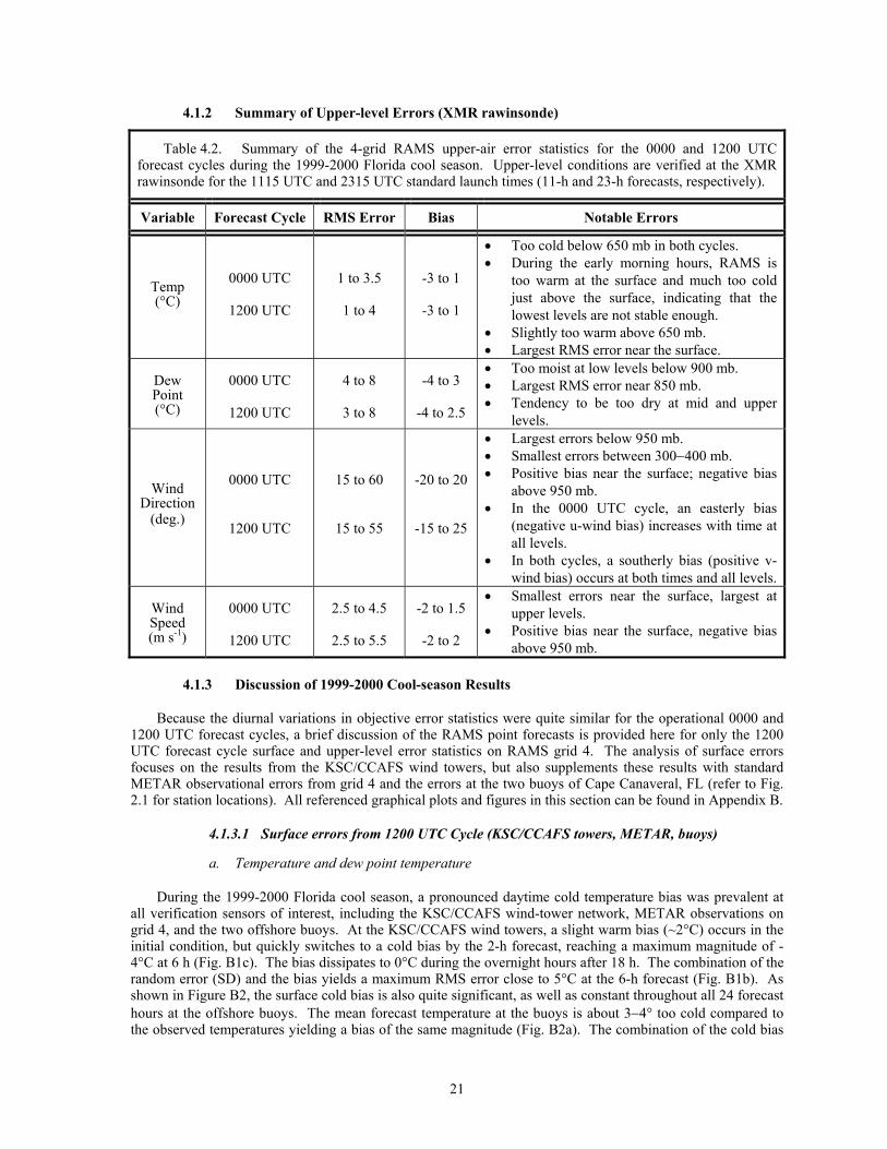
21

4.1.2 Summary of Upper-level Errors (XMR rawinsonde)

Table 4.2. Summary of the 4-grid RAMS upper-air error statistics for the 0000 and 1200 UTC forecast cycles during the 1999-2000 Florida cool season. Upper-level conditions are verified at the XMR rawinsonde for the 1115 UTC and 2315 UTC standard launch times (11-h and 23-h forecasts, respectively).

Variable Forecast Cycle RMS Error Bias Notable Errors

Temp (°C)

0000 UTC

1200 UTC

1 to 3.5

1 to 4

-3 to 1

-3 to 1

• Too cold below 650 mb in both cycles. • During the early morning hours, RAMS is

too warm at the surface and much too cold just above the surface, indicating that the lowest levels are not stable enough.

• Slightly too warm above 650 mb. • Largest RMS error near the surface.

Dew Point (°C)

0000 UTC

1200 UTC

4 to 8

3 to 8

-4 to 3

-4 to 2.5

• Too moist at low levels below 900 mb. • Largest RMS error near 850 mb. • Tendency to be too dry at mid and upper

levels.

Wind Direction

(deg.)

0000 UTC

1200 UTC

15 to 60

15 to 55

-20 to 20

-15 to 25

• Largest errors below 950 mb. • Smallest errors between 300−400 mb. • Positive bias near the surface; negative bias

above 950 mb. • In the 0000 UTC cycle, an easterly bias

(negative u-wind bias) increases with time at all levels.

• In both cycles, a southerly bias (positive v-wind bias) occurs at both times and all levels.

Wind Speed (m s-1)

0000 UTC

1200 UTC

2.5 to 4.5

2.5 to 5.5

-2 to 1.5

-2 to 2

• Smallest errors near the surface, largest at upper levels.

• Positive bias near the surface, negative bias above 950 mb.

4.1.3 Discussion of 1999-2000 Cool-season Results

Because the diurnal variations in objective error statistics were quite similar for the operational 0000 and 1200 UTC forecast cycles, a brief discussion of the RAMS point forecasts is provided here for only the 1200 UTC forecast cycle surface and upper-level error statistics on RAMS grid 4. The analysis of surface errors focuses on the results from the KSC/CCAFS wind towers, but also supplements these results with standard METAR observational errors from grid 4 and the errors at the two buoys of Cape Canaveral, FL (refer to Fig. 2.1 for station locations). All referenced graphical plots and figures in this section can be found in Appendix B.

4.1.3.1 Surface errors from 1200 UTC Cycle (KSC/CCAFS towers, METAR, buoys)

a. Temperature and dew point temperature

During the 1999-2000 Florida cool season, a pronounced daytime cold temperature bias was prevalent at all verification sensors of interest, including the KSC/CCAFS wind-tower network, METAR observations on grid 4, and the two offshore buoys. At the KSC/CCAFS wind towers, a slight warm bias (~2°C) occurs in the initial condition, but quickly switches to a cold bias by the 2-h forecast, reaching a maximum magnitude of -4°C at 6 h (Fig. B1c). The bias dissipates to 0°C during the overnight hours after 18 h. The combination of the random error (SD) and the bias yields a maximum RMS error close to 5°C at the 6-h forecast (Fig. B1b). As shown in Figure B2, the surface cold bias is also quite significant, as well as constant throughout all 24 forecast hours at the offshore buoys. The mean forecast temperature at the buoys is about 3−4° too cold compared to the observed temperatures yielding a bias of the same magnitude (Fig. B2a). The combination of the cold bias

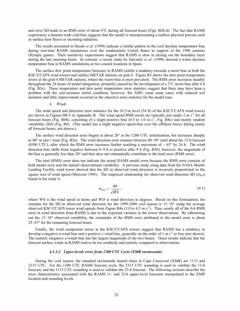
22

and error SD leads to an RMS error of about 4°C during all forecast hours (Figs. B2b-d). The fact that RAMS experiences a domain-wide cold bias suggests that the model is misrepresenting a surface physical process such as surface heat fluxes or incoming radiation.

The results presented in Snook et al. (1998) indicate a similar pattern in the cool daytime temperature bias during real-time RAMS simulations over the southeastern United States in support of the 1996 summer Olympic games. Their sensitivity experiments suggest that RAMS is slow in mixing out the boundary layer during the late morning hours. In contrast, a recent study by Salvador et al. (1999) showed a warm daytime temperature bias in RAMS simulations at two coastal locations in Spain.

The surface dew point temperature forecasts in RAMS exhibit a tendency towards a moist bias at both the KSC/CCAFS wind towers and surface METAR stations on grid 4. Figure B3 shows the dew point temperature errors at the grid-4 METAR stations, where the warm bias is most prevalent. The RMS error increases steadily throughout the 24 hours of model integration, primarily caused by the development of a 2°C moist bias after 6 h (Fig. B3c). These temperature and dew point temperature error statistics suggest that there may have been a problem with the soil-moisture initial condition; however, the AMU reran some cases with reduced soil moisture and little improvement occurred in the objective error statistics for the model runs.

b. Winds

The wind speed and direction error statistics for the 16.5-m level (54 ft) of the KSC/CCAFS wind towers are shown in Figures B4-5 in Appendix B. The wind speed RMS errors are typically just under 2 m s-1 for all forecast hours (Fig. B4b), consisting of a slight positive bias (0.5 to 1.0 m s-1, Fig. B4c) and mostly random variability (SD) (Fig. B4). (The model has a slight negative speed bias over the offshore buoys during nearly all forecast hours, not shown.).

The surface wind direction error begins at about 20° at the 1200 UTC initialization, but increases sharply to 40° in just 1 hour (Fig. B5a). The wind direction error remains between 40−50° until about the 15-h forecast (0300 UTC), after which the RMS error increases further reaching a maximum of ~ 65° by 24 h. The wind direction bias shifts from negative between 0−9 h to positive after 9 h (Fig. B5b); however, the magnitude of the bias is generally less than 20° and thus does not substantially contribute to the total error (RMS error).

The total (RMS) error does not indicate the actual RAMS model error because the RMS error consists of both model error and the natural observational variability. A previous study using data from the NASA Shuttle Landing Facility wind tower showed that the SD in observed wind direction is inversely proportional to the square root of wind speed (Merceret 1995). The empirical relationship for observed wind direction SD (σWD) found in his study is

WSWD44

=σ , (4.1)

where WS is the wind speed in knots and WD is wind direction in degrees. Based on this formulation, the estimate for the SD in observed wind direction for the 1999-2000 cool season is 15–18° using the average observed KSC/CCAFS tower wind speeds from Figure B4a (3.0 to 4.3 m s-1). Thus, nearly all of the 0-h RMS error in wind direction from RAMS is due to the expected variance in the tower observations. By subtracting out the 15−18° observed variability, the remainder of the RMS error attributed to the model error is about 25−47° for the remaining forecast hours.

Finally, the wind component errors at the KSC/CCAFS towers suggest that RAMS has a tendency to develop a negative u-wind bias and a positive v-wind bias, generally on the order of 1 m s-1 or less (not shown). The easterly (negative u-wind) bias has the largest magnitude of the two biases. These results indicate that the forecast surface winds in RAMS tend to be too southerly and easterly compared to observations.

4.1.3.2 Upper-levels error from 1200 UTC Cycle (XMR rawinsonde)

During the cool season, the standard rawinsonde launch times at Cape Canaveral (XMR) are 1115 and 2315 UTC. For the 1200 UTC RAMS forecast cycle, the 2315 UTC sounding is used to validate the 11-h forecast, and the 1115 UTC sounding is used to validate the 23-h forecast. The following sections describe the error characteristics associated with the RAMS 11- and 23-h upper-level forecasts interpolated to the XMR location and sounding levels.

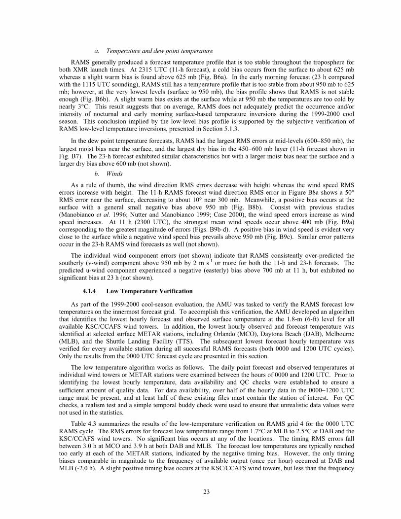
23

a. Temperature and dew point temperature

RAMS generally produced a forecast temperature profile that is too stable throughout the troposphere for both XMR launch times. At 2315 UTC (11-h forecast), a cold bias occurs from the surface to about 625 mb whereas a slight warm bias is found above 625 mb (Fig. B6a). In the early morning forecast (23 h compared with the 1115 UTC sounding), RAMS still has a temperature profile that is too stable from about 950 mb to 625 mb; however, at the very lowest levels (surface to 950 mb), the bias profile shows that RAMS is not stable enough (Fig. B6b). A slight warm bias exists at the surface while at 950 mb the temperatures are too cold by nearly 3°C. This result suggests that on average, RAMS does not adequately predict the occurrence and/or intensity of nocturnal and early morning surface-based temperature inversions during the 1999-2000 cool season. This conclusion implied by the low-level bias profile is supported by the subjective verification of RAMS low-level temperature inversions, presented in Section 5.1.3.

In the dew point temperature forecasts, RAMS had the largest RMS errors at mid-levels (600−850 mb), the largest moist bias near the surface, and the largest dry bias in the 450−600 mb layer (11-h forecast shown in Fig. B7). The 23-h forecast exhibited similar characteristics but with a larger moist bias near the surface and a larger dry bias above 600 mb (not shown).

b. Winds

As a rule of thumb, the wind direction RMS errors decrease with height whereas the wind speed RMS errors increase with height. The 11-h RAMS forecast wind direction RMS error in Figure B8a shows a 50° RMS error near the surface, decreasing to about 10° near 300 mb. Meanwhile, a positive bias occurs at the surface with a general small negative bias above 950 mb (Fig. B8b). Consist with previous studies (Manobianco et al. 1996; Nutter and Manobianco 1999; Case 2000), the wind speed errors increase as wind speed increases. At 11 h (2300 UTC), the strongest mean wind speeds occur above 400 mb (Fig. B9a) corresponding to the greatest magnitude of errors (Figs. B9b-d). A positive bias in wind speed is evident very close to the surface while a negative wind speed bias prevails above 950 mb (Fig. B9c). Similar error patterns occur in the 23-h RAMS wind forecasts as well (not shown).

The individual wind component errors (not shown) indicate that RAMS consistently over-predicted the southerly (v-wind) component above 950 mb by 2 m s-1 or more for both the 11-h and 23-h forecasts. The predicted u-wind component experienced a negative (easterly) bias above 700 mb at 11 h, but exhibited no significant bias at 23 h (not shown).

4.1.4 Low Temperature Verification

As part of the 1999-2000 cool-season evaluation, the AMU was tasked to verify the RAMS forecast low temperatures on the innermost forecast grid. To accomplish this verification, the AMU developed an algorithm that identifies the lowest hourly forecast and observed surface temperature at the 1.8-m (6-ft) level for all available KSC/CCAFS wind towers. In addition, the lowest hourly observed and forecast temperature was identified at selected surface METAR stations, including Orlando (MCO), Daytona Beach (DAB), Melbourne (MLB), and the Shuttle Landing Facility (TTS). The subsequent lowest forecast hourly temperature was verified for every available station during all successful RAMS forecasts (both 0000 and 1200 UTC cycles). Only the results from the 0000 UTC forecast cycle are presented in this section.

The low temperature algorithm works as follows. The daily point forecast and observed temperatures at individual wind towers or METAR stations were examined between the hours of 0000 and 1200 UTC. Prior to identifying the lowest hourly temperature, data availability and QC checks were established to ensure a sufficient amount of quality data. For data availability, over half of the hourly data in the 0000−1200 UTC range must be present, and at least half of these existing files must contain the station of interest. For QC checks, a realism test and a simple temporal buddy check were used to ensure that unrealistic data values were not used in the statistics.

Table 4.3 summarizes the results of the low-temperature verification on RAMS grid 4 for the 0000 UTC RAMS cycle. The RMS errors for forecast low temperature range from 1.7°C at MLB to 2.5°C at DAB and the KSC/CCAFS wind towers. No significant bias occurs at any of the locations. The timing RMS errors fall between 3.0 h at MCO and 3.9 h at both DAB and MLB. The forecast low temperatures are typically reached too early at each of the METAR stations, indicated by the negative timing bias. However, the only timing biases comparable in magnitude to the frequency of available output (once per hour) occurred at DAB and MLB (-2.0 h). A slight positive timing bias occurs at the KSC/CCAFS wind towers, but less than the frequency

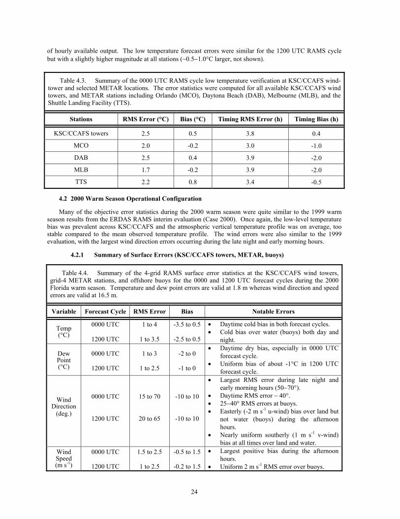
24

of hourly available output. The low temperature forecast errors were similar for the 1200 UTC RAMS cycle but with a slightly higher magnitude at all stations (~0.5−1.0°C larger, not shown).

Table 4.3. Summary of the 0000 UTC RAMS cycle low temperature verification at KSC/CCAFS wind-tower and selected METAR locations. The error statistics were computed for all available KSC/CCAFS wind towers, and METAR stations including Orlando (MCO), Daytona Beach (DAB), Melbourne (MLB), and the Shuttle Landing Facility (TTS).

Stations RMS Error (°C) Bias (°C) Timing RMS Error (h) Timing Bias (h)

KSC/CCAFS towers 2.5 0.5 3.8 0.4

MCO 2.0 -0.2 3.0 -1.0

DAB 2.5 0.4 3.9 -2.0

MLB 1.7 -0.2 3.9 -2.0

TTS 2.2 0.8 3.4 -0.5

4.2 2000 Warm Season Operational Configuration

Many of the objective error statistics during the 2000 warm season were quite similar to the 1999 warm season results from the ERDAS RAMS interim evaluation (Case 2000). Once again, the low-level temperature bias was prevalent across KSC/CCAFS and the atmospheric vertical temperature profile was on average, too stable compared to the mean observed temperature profile. The wind errors were also similar to the 1999 evaluation, with the largest wind direction errors occurring during the late night and early morning hours.

4.2.1 Summary of Surface Errors (KSC/CCAFS towers, METAR, buoys)

Table 4.4. Summary of the 4-grid RAMS surface error statistics at the KSC/CCAFS wind towers, grid-4 METAR stations, and offshore buoys for the 0000 and 1200 UTC forecast cycles during the 2000 Florida warm season. Temperature and dew point errors are valid at 1.8 m whereas wind direction and speed errors are valid at 16.5 m.

Variable Forecast Cycle RMS Error Bias Notable Errors

Temp (°C)

0000 UTC

1200 UTC

1 to 4

1 to 3.5

-3.5 to 0.5

-2.5 to 0.5

• Daytime cold bias in both forecast cycles. • Cold bias over water (buoys) both day and

night.

Dew Point (°C)

0000 UTC

1200 UTC

1 to 3

1 to 2.5

-2 to 0

-1 to 0

• Daytime dry bias, especially in 0000 UTC forecast cycle.

• Uniform bias of about -1°C in 1200 UTC forecast cycle.

Wind Direction

(deg.)

0000 UTC

1200 UTC

15 to 70

20 to 65

-10 to 10

-10 to 10

• Largest RMS error during late night and early morning hours (50−70°).

• Daytime RMS error ~ 40°. • 25−40° RMS errors at buoys. • Easterly (-2 m s-1 u-wind) bias over land but

not water (buoys) during the afternoon hours.

• Nearly uniform southerly (1 m s-1 v-wind) bias at all times over land and water.

Wind Speed (m s-1)

0000 UTC

1200 UTC

1.5 to 2.5

1 to 2.5

-0.5 to 1.5

-0.2 to 1.5

• Largest positive bias during the afternoon hours.

• Uniform 2 m s-1 RMS error over buoys.

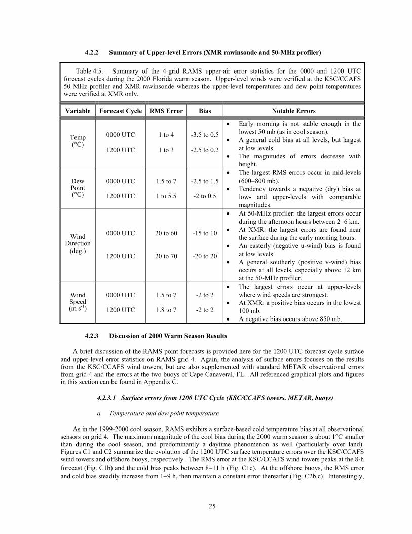
25

4.2.2 Summary of Upper-level Errors (XMR rawinsonde and 50-MHz profiler)

Table 4.5. Summary of the 4-grid RAMS upper-air error statistics for the 0000 and 1200 UTC forecast cycles during the 2000 Florida warm season. Upper-level winds were verified at the KSC/CCAFS 50 MHz profiler and XMR rawinsonde whereas the upper-level temperatures and dew point temperatures were verified at XMR only.

Variable Forecast Cycle RMS Error Bias Notable Errors

Temp (°C)

0000 UTC

1200 UTC

1 to 4

1 to 3

-3.5 to 0.5

-2.5 to 0.2

• Early morning is not stable enough in the lowest 50 mb (as in cool season).

• A general cold bias at all levels, but largest at low levels.

• The magnitudes of errors decrease with height.

Dew Point (°C)

0000 UTC

1200 UTC

1.5 to 7

1 to 5.5

-2.5 to 1.5

-2 to 0.5

• The largest RMS errors occur in mid-levels (600−800 mb).

• Tendency towards a negative (dry) bias at low- and upper-levels with comparable magnitudes.

Wind Direction

(deg.)

0000 UTC

1200 UTC

20 to 60

20 to 70

-15 to 10

-20 to 20

• At 50-MHz profiler: the largest errors occur during the afternoon hours between 2−6 km.

• At XMR: the largest errors are found near the surface during the early morning hours.

• An easterly (negative u-wind) bias is found at low levels.

• A general southerly (positive v-wind) bias occurs at all levels, especially above 12 km at the 50-MHz profiler.

Wind Speed (m s-1)

0000 UTC

1200 UTC

1.5 to 7

1.8 to 7

-2 to 2

-2 to 2

• The largest errors occur at upper-levels where wind speeds are strongest.

• At XMR: a positive bias occurs in the lowest 100 mb.

• A negative bias occurs above 850 mb.

4.2.3 Discussion of 2000 Warm Season Results

A brief discussion of the RAMS point forecasts is provided here for the 1200 UTC forecast cycle surface and upper-level error statistics on RAMS grid 4. Again, the analysis of surface errors focuses on the results from the KSC/CCAFS wind towers, but are also supplemented with standard METAR observational errors from grid 4 and the errors at the two buoys of Cape Canaveral, FL. All referenced graphical plots and figures in this section can be found in Appendix C.

4.2.3.1 Surface errors from 1200 UTC Cycle (KSC/CCAFS towers, METAR, buoys)

a. Temperature and dew point temperature

As in the 1999-2000 cool season, RAMS exhibits a surface-based cold temperature bias at all observational sensors on grid 4. The maximum magnitude of the cool bias during the 2000 warm season is about 1°C smaller than during the cool season, and predominantly a daytime phenomenon as well (particularly over land). Figures C1 and C2 summarize the evolution of the 1200 UTC surface temperature errors over the KSC/CCAFS wind towers and offshore buoys, respectively. The RMS error at the KSC/CCAFS wind towers peaks at the 8-h forecast (Fig. C1b) and the cold bias peaks between 8−11 h (Fig. C1c). At the offshore buoys, the RMS error and cold bias steadily increase from 1−9 h, then maintain a constant error thereafter (Fig. C2b,c). Interestingly,

26

the random component of the errors (SD) at the buoys remains nearly constant during all 24 forecast hours (Fig. C2d).

Contrary to the 1999-2000 cool season, the RAMS surface dew point temperature errors indicate a small dry bias at the KSC/CCAFS wind towers, as shown in Figure C3. The model consistently has about a -1°C dry bias at nearly all forecast hours. Meanwhile, the RMS error and SD grow only about 1°C from 0−6 h, then maintain a constant error thereafter.

b. Winds

The RAMS forecast wind speeds at the KSC/CCAFS contain a 1−2 m s-1 positive bias, primarily during the afternoon and evening hours (4−15 h in Fig. C4c). The ECSB typically propagates westward through the KSC/CCAFS tower network during the late morning and early afternoon hours (1500−1800 UTC, Cetola 1997) corresponding to the 3−6-h forecasts from the 1200 UTC RAMS run. These results suggest that the forecast wind speeds are slightly too strong following the passage of the ECSB. Both the RMS error and SD steadily grow from initialization to 9 h, then decrease thereafter (Figs. C4b,d). At the two offshore buoys, the RMS error and SD are nearly constant at 2 m s-1 during all 24 forecast hours with virtually no bias prevalent (not shown).

The wind direction errors at the KSC/CCAFS towers are given in Figure C5 and show a rapid growth in RMS error from 20−40° between initialization and the 2-h forecast. After 2 h, the RMS error remains at or slightly above 40° through 18 h (0600 UTC), after which the errors grow rapidly to about 60−65° (Fig. C5a). This peak in surface wind direction RMS error occurs during the light and variable wind regime of the late night and early morning hours, possibly caused by an inability of RAMS to predict adequately the return flow associated with nocturnal land breezes. Only a negligible bias occurs with a magnitude less than 10° (Fig. C5b).

To obtain the approximate portion of the RMS error attributed to the model, the same exercise is conducted with the wind direction RMS errors as in the 1999-2000 cool season. Using Eq. (4.1) and the mean observed surface wind speeds for the 2000 warm season (ranging from 2.2 to 4.2 m s-1 in Fig. C4a), the average variability in the observed wind direction at the KSC/CCAFS wind towers is about 15−21° for all forecast hours. The observed variability is largest during the late night and early morning hours when wind speeds are lightest. By subtracting the 15−21° observational variability from the range of total RMS error after initialization (40−65°), the resulting model RMS error is about 25−44°. These errors may result from the model's inability to resolve explicitly small-scale turbulent eddies, especially those associated with the light and variable winds during the nocturnal and early morning hours. In addition, a more sophisticated initialization scheme, such as four-dimensional data assimilation, may reduce the growth rate of these wind direction errors between 0−2 h by better incorporating the high-resolution observational data available in east-central Florida.

Finally, by examining the u-wind component errors of Figure C6, it becomes evident that RAMS over-predicts the magnitude of the easterly wind component following the sea-breeze passage at the KSC/CCAFS wind-tower network. During the afternoon and evening hours (4−14 h), corresponding to the times of the mean post-sea breeze regime, the forecast u-wind component experiences a 1−2 m s-1 easterly bias, peaking at 7 h (Fig. C6c).

4.2.3.2 Upper-levels error from 1200 UTC Cycle (XMR rawinsonde, 50 MHz profiler)

During the warm season, the standard rawinsonde launch times at Cape Canaveral (XMR) are 1015, 1500, and 2215 UTC. For the 1200 UTC RAMS forecast cycle, the 1500 UTC sounding is used to validate the 3-h forecast, the 2215 UTC sounding is used to validate the 10-h forecast, and the 1015 UTC sounding is used to validate the 22-h forecast. In addition, the 50-MHz DRWP data from the top of the each hour are used to verify RAMS wind forecasts from about 2−16-km height. The following sections describe the upper-level error characteristics associated with the RAMS 3-, 10- and 22-h forecasts interpolated to the XMR sounding levels, and the RAMS forecasts at all hours interpolated to the 50-MHz DRWP levels.

a. Temperature and dew point temperature

The forecasts at 3, 10, and 22 h all show that RAMS predicts a temperature profile that is too stable relative to observations, similar to the 1999-2000 cool-season results. Figure C7 shows the 10-h forecast errors (valid

27

2200 UTC) as a function of pressure at XMR. The main contributor to the overly stable forecast profile is a substantial cool bias below 650 mb that steadily increases to a maximum at the surface (Fig. C7c). As a result the RMS error also increases from 650 mb down to the surface (Fig. C7b). The temperature errors are nearly constant above 650 mb in the 10-h forecast as well as the 3-h and 22-h forecasts (not shown). Except for the surface, the SD of the errors is nearly constant at about 1°C as a function of height for all three forecast times at about 1°C. Thus, the primary contributor to the growth of the total error at low levels is the model’s systematic cold error.

The profile of dew point temperature errors during the 2000 warm season is also quite similar to the error profile during the 1999-2000 cool season. In all three forecast times verified at XMR, the dew point errors are smallest near the surface (1.5−3.0°C) and increase with height reaching a maximum of 5−6°C between 600−800 mb, then decrease above 600 mb (not shown). The errors are composed of primarily random variability since the SD is quite similar to the RMS error and the biases are small in magnitude relative to the RMS error.

b. Winds

The errors in wind speed and wind direction exhibit a similar pattern to the 1999-2000 cool-season errors, but the change in magnitude of the errors as a function of height is not as pronounced as the cool season, particularly with wind direction. In the lowest 2 km (roughly surface to 800 mb) at XMR, the magnitude of the wind speed errors increase slightly with time from about 2 m s-1 at the 3-h forecast to 2.5 m s-1 at the 10-h and 22-h forecasts (not shown). The wind speed errors are nearly constant with height in the lowest 2 km as well.

Above 2 km, the wind speeds can be verified against the 50-MHz DRWP on an hourly basis. Figure C8 shows a time-height cross section of RAMS wind speed errors at the 50-MHz DRWP location. By comparing the mean observed and forecast wind speeds in Figures C8a and b, it appears that the RAMS wind speeds are slightly weaker than the observed speeds. The plot in Figure C8d reveals a 1−2 m s-1 negative bias at nearly all levels particularly after the 12-h forecast. Meanwhile, the total error in Figure C8c depicts an increase in RMS error with height reaching a maximum between 12−14 km, corresponding to the axis of maximum observed wind speed.

The wind direction errors verified at XMR in the lowest 2 km (roughly surface to 800 mb) indicate that RAMS forecasts have the largest errors near the surface for the 3-h and 22-h forecasts (1500 and 1000 UTC respectively shown in Figs. C9a and C11a). At these times, the RMS error decreases with height from the surface to 800 mb. Meanwhile, the wind direction errors during the late afternoon, post-sea breeze regime have a much different profile between the surface and 800 mb (Fig C10). During the mean post-sea breeze regime, the wind direction RMS errors increase from about 30° near the surface to about 50−55° between 800−900 mb. This late-afternoon error structure could result from consist accurate predictions of the sea-breeze onset and propagation across east-central Florida near the surface (refer to the results of the east-coast sea-breeze subjective verification in Section 5.2.1), combined with uncertainty in the depth of the sea-breeze circulation.

The wind direction verification above 2 km at the 50-MHz profiler is shown in Figure C12. A general increase in the RMS error occurs in the first 6 forecast hours at nearly all vertical levels (Fig. C12a). Most of the errors are between 30−50° for all levels and forecast hours at the 50-MHz DRWP. The magnitude of the bias is typically 10° or less (Fig. C12b) and thus, substantially less than the magnitude of the RMS error. As a result, most of the errors are composed of random variability.

The wind component errors do not have many extraordinary characteristics that are substantially different from the wind speed and direction errors. The RMS errors increase with height for both wind components (as in the wind speed) and only a 1 m s-1 easterly bias occurs below 950 mb in the 10-h forecast at XMR (not shown). The v-wind component tends to have the largest bias at all times and levels, especially in the lowest levels of the atmosphere. Generally, a 1−2 m s-1 southerly bias is evident with the greatest bias occurring in the 10-h forecast below 800 mb at XMR (not shown).

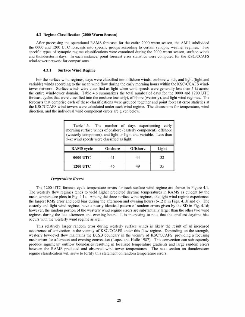
28

4.3 Regime Classification (2000 Warm Season)

After processing the operational RAMS forecasts for the entire 2000 warm season, the AMU subdivided the 0000 and 1200 UTC forecasts into specific groups according to certain synoptic weather regimes. Two specific types of synoptic regime classifications were examined during the 2000 warm season, surface winds and thunderstorm days. In each instance, point forecast error statistics were computed for the KSC/CCAFS wind-tower network for comparisons.

4.3.1 Surface Wind Regime

For the surface wind regimes, days were classified into offshore winds, onshore winds, and light (light and variable) winds according to the mean wind flow during the early morning hours within the KSC/CCAFS wind-tower network. Surface winds were classified as light when wind speeds were generally less than 5 kt across the entire wind-tower domain. Table 4.6 summarizes the total number of days for the 0000 and 1200 UTC forecast cycles that were classified into the onshore (easterly), offshore (westerly), and light wind regimes. The forecasts that comprise each of these classifications were grouped together and point forecast error statistics at the KSC/CCAFS wind towers were calculated under each wind regime. The discussions for temperature, wind direction, and the individual wind component errors are given below.

Table 4.6. The number of days experiencing early morning surface winds of onshore (easterly component), offshore (westerly component), and light or light and variable. Less than 5-kt wind speeds were classified as light.

RAMS cycle Onshore Offshore Light

0000 UTC 41 44 32

1200 UTC 46 49 35

Temperature Errors

The 1200 UTC forecast cycle temperature errors for each surface wind regime are shown in Figure 4.1. The westerly flow regimes tends to yield higher predicted daytime temperatures in RAMS as evident by the mean temperature plots in Fig. 4.1a. Among the three surface wind regimes, the light wind regime experiences the largest RMS error and cold bias during the afternoon and evening hours (6-12 h in Figs. 4.1b and c). The easterly and light wind regimes have a nearly identical pattern of random errors given by the SD in Fig. 4.1d; however, the random portion of the westerly wind regime errors are substantially larger than the other two wind regimes during the late afternoon and evening hours. It is interesting to note that the smallest daytime bias occurs with the westerly wind regime as well.

This relatively larger random error during westerly surface winds is likely the result of an increased occurrence of convection in the vicinity of KSC/CCAFS under this flow regime. Depending on the strength, westerly low-level flow maintains the ECSB boundary in the vicinity of KSC/CCAFS, providing a focusing mechanism for afternoon and evening convection (López and Holle 1987). This convection can subsequently produce significant outflow boundaries resulting in localized temperature gradients and large random errors between the RAMS predicted and observed wind-tower temperatures. The next section on thunderstorm regime classification will serve to fortify this statement on random temperature errors.

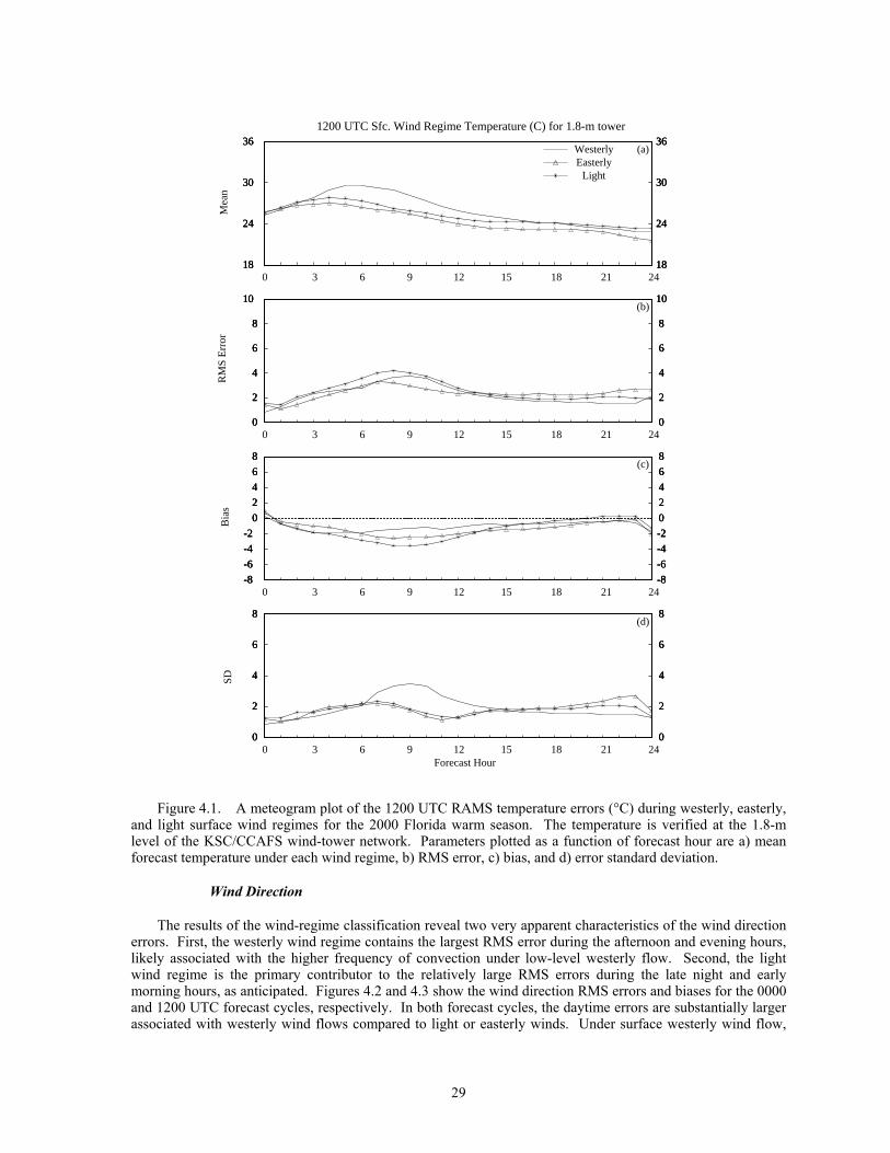
29

18

24

30

36

18

24

30

36

0

2

4

6

8

10

0

2

4

6

8

10

-8

-6

-4

-2

0

2

4

6

8

-8

-6

-4

-2

0

2

4

6

8

10/00 10/02 10/04 10/06 10/08 10/10 10/12 10/14 10/16 10/18 10/20 10/22 11/000

2

4

6

8

0

2

4

6

8

18

24

30

36

18

24

30

36

0

2

4

6

8

10

0

2

4

6

8

10

-8

-6

-4

-2

0

2

4

6

8

-8

-6

-4

-2

0

2

4

6

8

10/00 10/02 10/04 10/06 10/08 10/10 10/12 10/14 10/16 10/18 10/20 10/22 11/000

2

4

6

8

0

2

4

6

8

18

24

30

36

18

24

30

36

0

2

4

6

8

10

0

2

4

6

8

10

-8

-6

-4

-2

0

2

4

6

8

-8

-6

-4

-2

0

2

4

6

8

10/00 10/02 10/04 10/06 10/08 10/10 10/12 10/14 10/16 10/18 10/20 10/22 11/000

2

4

6

8

0

2

4

6

8

(a)WesterlyEasterly

(b)

(c)

(d)

Mea

nR

MS

Err

orB

ias

SD

0 3 6 9 12 15 18 21 24

0 3 6 9 12 15 18 21 24

0 3 6 9 12 15 18 21 24

0 3 6 9 12 15 18 21 24

Forecast Hour

1200 UTC Sfc. Wind Regime Temperature (C) for 1.8-m tower

Light

Figure 4.1. A meteogram plot of the 1200 UTC RAMS temperature errors (°C) during westerly, easterly,

and light surface wind regimes for the 2000 Florida warm season. The temperature is verified at the 1.8-m level of the KSC/CCAFS wind-tower network. Parameters plotted as a function of forecast hour are a) mean forecast temperature under each wind regime, b) RMS error, c) bias, and d) error standard deviation.

Wind Direction

The results of the wind-regime classification reveal two very apparent characteristics of the wind direction errors. First, the westerly wind regime contains the largest RMS error during the afternoon and evening hours, likely associated with the higher frequency of convection under low-level westerly flow. Second, the light wind regime is the primary contributor to the relatively large RMS errors during the late night and early morning hours, as anticipated. Figures 4.2 and 4.3 show the wind direction RMS errors and biases for the 0000 and 1200 UTC forecast cycles, respectively. In both forecast cycles, the daytime errors are substantially larger associated with westerly wind flows compared to light or easterly winds. Under surface westerly wind flow,

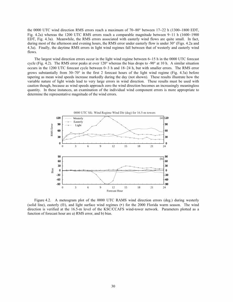
30

the 0000 UTC wind direction RMS errors reach a maximum of 70−80° between 17−22 h (1300−1800 EDT, Fig. 4.2a) whereas the 1200 UTC RMS errors reach a comparable magnitude between 9−11 h (1600−1900 EDT, Fig. 4.3a). Meanwhile, the RMS errors associated with easterly wind flows are quite small. In fact, during most of the afternoon and evening hours, the RMS error under easterly flow is under 30° (Figs. 4.2a and 4.3a). Finally, the daytime RMS errors in light wind regimes fall between that of westerly and easterly wind flows.

The largest wind direction errors occur in the light wind regime between 6−15 h in the 0000 UTC forecast cycle (Fig. 4.2). The RMS error peaks at over 120° whereas the bias drops to -90° at 10 h. A similar situation occurs in the 1200 UTC forecast cycle between 0−3 h and 18−24 h, but with smaller errors. The RMS error grows substantially from 30−70° in the first 2 forecast hours of the light wind regime (Fig. 4.3a) before tapering as mean wind speeds increase markedly during the day (not shown). These results illustrate how the variable nature of light winds lead to very large errors in wind direction. These results must be used with caution though, because as wind speeds approach zero the wind direction becomes an increasingly meaningless quantity. In these instances, an examination of the individual wind component errors is more appropriate to determine the representative magnitude of the wind errors.

0

30

60

90

120

0

30

60

90

120

10/00 10/02 10/04 10/06 10/08 10/10 10/12 10/14 10/16 10/18 10/20 10/22 11/00-90

-60

-30

0

30

60

90

-90

-60

-30

0

30

60

90

0

30

60

90

120

0

30

60

90

120

10/00 10/02 10/04 10/06 10/08 10/10 10/12 10/14 10/16 10/18 10/20 10/22 11/00-90

-60

-30

0

30

60

90

-90

-60

-30

0

30

60

90

0

30

60

90

120

0

30

60

90

120

10/00 10/02 10/04 10/06 10/08 10/10 10/12 10/14 10/16 10/18 10/20 10/22 11/00-90

-60

-30

0

30

60

90

-90

-60

-30

0

30

60

90

(a)

(b)

RM

S E

rror

Bia

s

0 3 6 9 12 15 18 21 24

0 3 6 9 12 15 18 21 24

Forecast Hour

WesterlyEasterly

Light

0000 UTC Sfc. Wind Regime Wind Dir (deg) for 16.5-m towers

Figure 4.2. A meteogram plot of the 0000 UTC RAMS wind direction errors (deg.) during westerly

(solid line), easterly (⊗), and light surface wind regimes (∗) for the 2000 Florida warm season. The wind direction is verified at the 16.5-m level of the KSC/CCAFS wind-tower network. Parameters plotted as a function of forecast hour are a) RMS error, and b) bias.

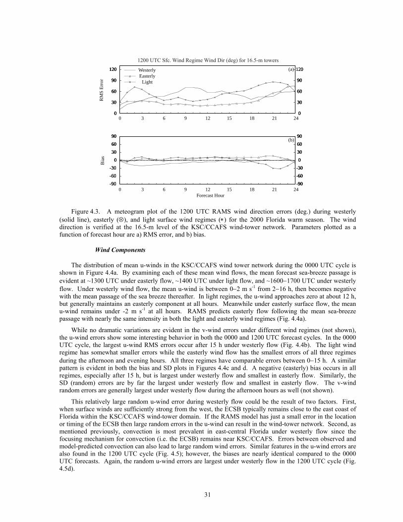
31

0

30

60

90

120

0

30

60

90

120

10/00 10/02 10/04 10/06 10/08 10/10 10/12 10/14 10/16 10/18 10/20 10/22 11/00-90

-60

-30

0

30

60

90

-90

-60

-30

0

30

60

90

0

30

60

90

120

0

30

60

90

120

10/00 10/02 10/04 10/06 10/08 10/10 10/12 10/14 10/16 10/18 10/20 10/22 11/00-90

-60

-30

0

30

60

90

-90

-60

-30

0

30

60

90

0

30

60

90

120

0

30

60

90

120

10/00 10/02 10/04 10/06 10/08 10/10 10/12 10/14 10/16 10/18 10/20 10/22 11/00-90

-60

-30

0

30

60

90

-90

-60

-30

0

30

60

90

(a)

(b)

RM

S E

rror

Bia

s

0 3 6 9 12 15 18 21 24

0 3 6 9 12 15 18 21 24

Forecast Hour

WesterlyEasterly

Light

1200 UTC Sfc. Wind Regime Wind Dir (deg) for 16.5-m towers

Figure 4.3. A meteogram plot of the 1200 UTC RAMS wind direction errors (deg.) during westerly

(solid line), easterly (⊗), and light surface wind regimes (∗) for the 2000 Florida warm season. The wind direction is verified at the 16.5-m level of the KSC/CCAFS wind-tower network. Parameters plotted as a function of forecast hour are a) RMS error, and b) bias.

Wind Components

The distribution of mean u-winds in the KSC/CCAFS wind tower network during the 0000 UTC cycle is shown in Figure 4.4a. By examining each of these mean wind flows, the mean forecast sea-breeze passage is evident at ~1300 UTC under easterly flow, ~1400 UTC under light flow, and ~1600−1700 UTC under westerly flow. Under westerly wind flow, the mean u-wind is between 0−2 m s-1 from 2−16 h, then becomes negative with the mean passage of the sea breeze thereafter. In light regimes, the u-wind approaches zero at about 12 h, but generally maintains an easterly component at all hours. Meanwhile under easterly surface flow, the mean u-wind remains under -2 m s-1 at all hours. RAMS predicts easterly flow following the mean sea-breeze passage with nearly the same intensity in both the light and easterly wind regimes (Fig. 4.4a).

While no dramatic variations are evident in the v-wind errors under different wind regimes (not shown), the u-wind errors show some interesting behavior in both the 0000 and 1200 UTC forecast cycles. In the 0000 UTC cycle, the largest u-wind RMS errors occur after 15 h under westerly flow (Fig. 4.4b). The light wind regime has somewhat smaller errors while the easterly wind flow has the smallest errors of all three regimes during the afternoon and evening hours. All three regimes have comparable errors between 0−15 h. A similar pattern is evident in both the bias and SD plots in Figures 4.4c and d. A negative (easterly) bias occurs in all regimes, especially after 15 h, but is largest under westerly flow and smallest in easterly flow. Similarly, the SD (random) errors are by far the largest under westerly flow and smallest in easterly flow. The v-wind random errors are generally largest under westerly flow during the afternoon hours as well (not shown).

This relatively large random u-wind error during westerly flow could be the result of two factors. First, when surface winds are sufficiently strong from the west, the ECSB typically remains close to the east coast of Florida within the KSC/CCAFS wind-tower domain. If the RAMS model has just a small error in the location or timing of the ECSB then large random errors in the u-wind can result in the wind-tower network. Second, as mentioned previously, convection is most prevalent in east-central Florida under westerly flow since the focusing mechanism for convection (i.e. the ECSB) remains near KSC/CCAFS. Errors between observed and model-predicted convection can also lead to large random wind errors. Similar features in the u-wind errors are also found in the 1200 UTC cycle (Fig. 4.5); however, the biases are nearly identical compared to the 0000 UTC forecasts. Again, the random u-wind errors are largest under westerly flow in the 1200 UTC cycle (Fig. 4.5d).

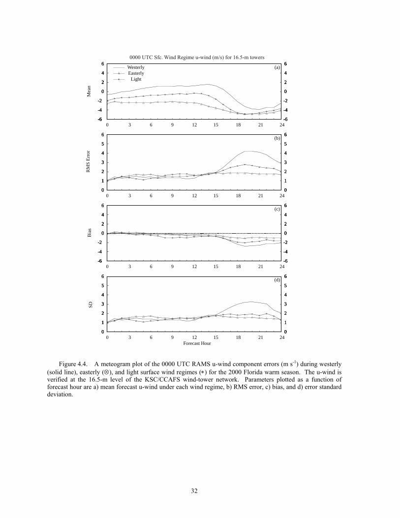
32

-6

-4

-2

0

2

4

6

-6

-4

-2

0

2

4

6

0

1

2

3

4

5

6

0

1

2

3

4

5

6

-6

-4

-2

0

2

4

6

-6

-4

-2

0

2

4

6

10/00 10/02 10/04 10/06 10/08 10/10 10/12 10/14 10/16 10/18 10/20 10/22 11/000

1

2

3

4

5

6

0

1

2

3

4

5

6

-6

-4

-2

0

2

4

6

-6

-4

-2

0

2

4

6

0

1

2

3

4

5

6

0

1

2

3

4

5

6

-6

-4

-2

0

2

4

6

-6

-4

-2

0

2

4

6

10/00 10/02 10/04 10/06 10/08 10/10 10/12 10/14 10/16 10/18 10/20 10/22 11/000

1

2

3

4

5

6

0

1

2

3

4

5

6

-6

-4

-2

0

2

4

6

-6

-4

-2

0

2

4

6

0

1

2

3

4

5

6

0

1

2

3

4

5

6

-6

-4

-2

0

2

4

6

-6

-4

-2

0

2

4

6

10/00 10/02 10/04 10/06 10/08 10/10 10/12 10/14 10/16 10/18 10/20 10/22 11/000

1

2

3

4

5

6

0

1

2

3

4

5

6

(a)WesterlyEasterly

(b)

(c)

(d)

Mea

nR

MS

Err

orB

ias

SD

0 3 6 9 12 15 18 21 24

0 3 6 9 12 15 18 21 24

0 3 6 9 12 15 18 21 24

0 3 6 9 12 15 18 21 24

Forecast Hour

Light

0000 UTC Sfc. Wind Regime u-wind (m/s) for 16.5-m towers

Figure 4.4. A meteogram plot of the 0000 UTC RAMS u-wind component errors (m s-1) during westerly

(solid line), easterly (⊗), and light surface wind regimes (∗) for the 2000 Florida warm season. The u-wind is verified at the 16.5-m level of the KSC/CCAFS wind-tower network. Parameters plotted as a function of forecast hour are a) mean forecast u-wind under each wind regime, b) RMS error, c) bias, and d) error standard deviation.

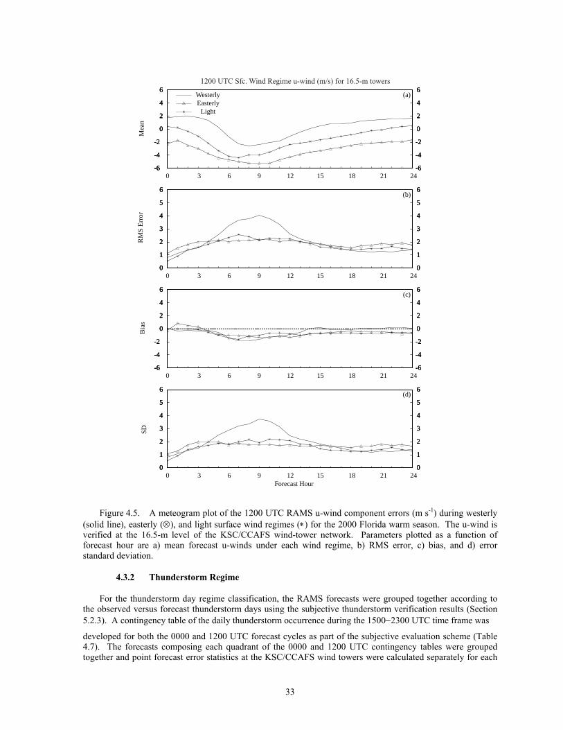
33

-6

-4

-2

0

2

4

6

-6

-4

-2

0

2

4

6

0

1

2

3

4

5

6

0

1

2

3

4

5

6

-6

-4

-2

0

2

4

6

-6

-4

-2

0

2

4

6

10/00 10/02 10/04 10/06 10/08 10/10 10/12 10/14 10/16 10/18 10/20 10/22 11/000

1

2

3

4

5

6

0

1

2

3

4

5

6

-6

-4

-2

0

2

4

6

-6

-4

-2

0

2

4

6

0

1

2

3

4

5

6

0

1

2

3

4

5

6

-6

-4

-2

0

2

4

6

-6

-4

-2

0

2

4

6

10/00 10/02 10/04 10/06 10/08 10/10 10/12 10/14 10/16 10/18 10/20 10/22 11/000

1

2

3

4

5

6

0

1

2

3

4

5

6

-6

-4

-2

0

2

4

6

-6

-4

-2

0

2

4

6

0

1

2

3

4

5

6

0

1

2

3

4

5

6

-6

-4

-2

0

2

4

6

-6

-4

-2

0

2

4

6

10/00 10/02 10/04 10/06 10/08 10/10 10/12 10/14 10/16 10/18 10/20 10/22 11/000

1

2

3

4

5

6

0

1

2

3

4

5

6

(a)WesterlyEasterly

(b)

(c)

(d)

Mea

nR

MS

Err

orB

ias

SD

0 3 6 9 12 15 18 21 24

0 3 6 9 12 15 18 21 24

0 3 6 9 12 15 18 21 24

0 3 6 9 12 15 18 21 24

Forecast Hour

Light

1200 UTC Sfc. Wind Regime u-wind (m/s) for 16.5-m towers

Figure 4.5. A meteogram plot of the 1200 UTC RAMS u-wind component errors (m s-1) during westerly

(solid line), easterly (⊗), and light surface wind regimes (∗) for the 2000 Florida warm season. The u-wind is verified at the 16.5-m level of the KSC/CCAFS wind-tower network. Parameters plotted as a function of forecast hour are a) mean forecast u-winds under each wind regime, b) RMS error, c) bias, and d) error standard deviation.

4.3.2 Thunderstorm Regime

For the thunderstorm day regime classification, the RAMS forecasts were grouped together according to the observed versus forecast thunderstorm days using the subjective thunderstorm verification results (Section 5.2.3). A contingency table of the daily thunderstorm occurrence during the 1500−2300 UTC time frame was

developed for both the 0000 and 1200 UTC forecast cycles as part of the subjective evaluation scheme (Table 4.7). The forecasts composing each quadrant of the 0000 and 1200 UTC contingency tables were grouped together and point forecast error statistics at the KSC/CCAFS wind towers were calculated separately for each

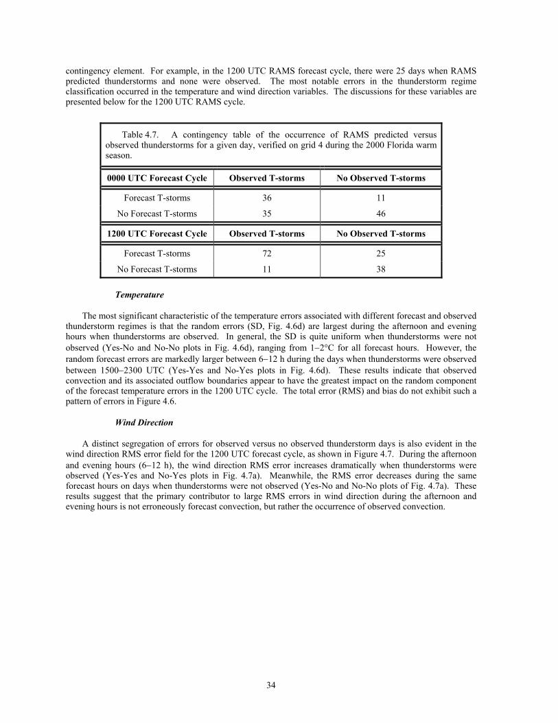
34

contingency element. For example, in the 1200 UTC RAMS forecast cycle, there were 25 days when RAMS predicted thunderstorms and none were observed. The most notable errors in the thunderstorm regime classification occurred in the temperature and wind direction variables. The discussions for these variables are presented below for the 1200 UTC RAMS cycle.

Table 4.7. A contingency table of the occurrence of RAMS predicted versus observed thunderstorms for a given day, verified on grid 4 during the 2000 Florida warm season.

0000 UTC Forecast Cycle Observed T-storms No Observed T-storms

Forecast T-storms 36 11

No Forecast T-storms 35 46

1200 UTC Forecast Cycle Observed T-storms No Observed T-storms

Forecast T-storms 72 25

No Forecast T-storms 11 38

Temperature

The most significant characteristic of the temperature errors associated with different forecast and observed thunderstorm regimes is that the random errors (SD, Fig. 4.6d) are largest during the afternoon and evening hours when thunderstorms are observed. In general, the SD is quite uniform when thunderstorms were not observed (Yes-No and No-No plots in Fig. 4.6d), ranging from 1−2°C for all forecast hours. However, the random forecast errors are markedly larger between 6−12 h during the days when thunderstorms were observed between 1500−2300 UTC (Yes-Yes and No-Yes plots in Fig. 4.6d). These results indicate that observed convection and its associated outflow boundaries appear to have the greatest impact on the random component of the forecast temperature errors in the 1200 UTC cycle. The total error (RMS) and bias do not exhibit such a pattern of errors in Figure 4.6.

Wind Direction

A distinct segregation of errors for observed versus no observed thunderstorm days is also evident in the wind direction RMS error field for the 1200 UTC forecast cycle, as shown in Figure 4.7. During the afternoon and evening hours (6−12 h), the wind direction RMS error increases dramatically when thunderstorms were observed (Yes-Yes and No-Yes plots in Fig. 4.7a). Meanwhile, the RMS error decreases during the same forecast hours on days when thunderstorms were not observed (Yes-No and No-No plots of Fig. 4.7a). These results suggest that the primary contributor to large RMS errors in wind direction during the afternoon and evening hours is not erroneously forecast convection, but rather the occurrence of observed convection.

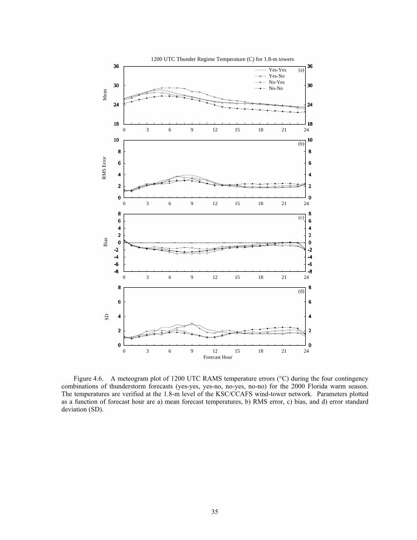
35

18

24

30

36

18

24

30

36

0

2

4

6

8

10

0

2

4

6

8

10

-8

-6

-4

-2

0

2

4

6

8

-8

-6

-4

-2

0

2

4

6

8

10/00 10/02 10/04 10/06 10/08 10/10 10/12 10/14 10/16 10/18 10/20 10/22 11/000

2

4

6

8

0

2

4

6

8

18

24

30

36

18

24

30

36

0

2

4

6

8

10

0

2

4

6

8

10

-8

-6

-4

-2

0

2

4

6

8

-8

-6

-4

-2

0

2

4

6

8

10/00 10/02 10/04 10/06 10/08 10/10 10/12 10/14 10/16 10/18 10/20 10/22 11/000

2

4

6

8

0

2

4

6

8

18

24

30

36

18

24

30

36

0

2

4

6

8

10

0

2

4

6

8

10

-8

-6

-4

-2

0

2

4

6

8

-8

-6

-4

-2

0

2

4

6

8

10/00 10/02 10/04 10/06 10/08 10/10 10/12 10/14 10/16 10/18 10/20 10/22 11/000

2

4

6

8

0

2

4

6

8

18

24

30

36

18

24

30

36

0

2

4

6

8

10

0

2

4

6

8

10

-8

-6

-4

-2

0

2

4

6

8

-8

-6

-4

-2

0

2

4

6

8

10/00 10/02 10/04 10/06 10/08 10/10 10/12 10/14 10/16 10/18 10/20 10/22 11/000

2

4

6

8

0

2

4

6

8

(a)Yes-YesYes-No

(b)

(c)

(d)

Mea

nR

MS

Err

orB

ias

SD

0 3 6 9 12 15 18 21 24

0 3 6 9 12 15 18 21 24

0 3 6 9 12 15 18 21 24

0 3 6 9 12 15 18 21 24

Forecast Hour

1200 UTC Thunder Regime Temperature (C) for 1.8-m towers

No-YesNo-No

Figure 4.6. A meteogram plot of 1200 UTC RAMS temperature errors (°C) during the four contingency

combinations of thunderstorm forecasts (yes-yes, yes-no, no-yes, no-no) for the 2000 Florida warm season. The temperatures are verified at the 1.8-m level of the KSC/CCAFS wind-tower network. Parameters plotted as a function of forecast hour are a) mean forecast temperatures, b) RMS error, c) bias, and d) error standard deviation (SD).

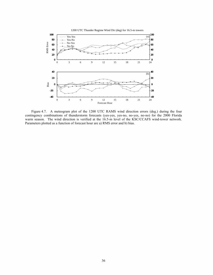
36

0

20

40

60

80

100

0

20

40

60

80

100

10/00 10/02 10/04 10/06 10/08 10/10 10/12 10/14 10/16 10/18 10/20 10/22 11/00-40

-20

0

20

40

-40

-20

0

20

40

0

20

40

60

80

100

0

20

40

60

80

100

10/00 10/02 10/04 10/06 10/08 10/10 10/12 10/14 10/16 10/18 10/20 10/22 11/00-40

-20

0

20

40

-40

-20

0

20

40

0

20

40

60

80

100

0

20

40

60

80

100

10/00 10/02 10/04 10/06 10/08 10/10 10/12 10/14 10/16 10/18 10/20 10/22 11/00-40

-20

0

20

40

-40

-20

0

20

40

0

20

40

60

80

100

0

20

40

60

80

100

10/00 10/02 10/04 10/06 10/08 10/10 10/12 10/14 10/16 10/18 10/20 10/22 11/00-40

-20

0

20

40

-40

-20

0

20

40

(a)

(b)

RM

S E

rror

Bia

s

0 3 6 9 12 15 18 21 24

0 3 6 9 12 15 18 21 24

Forecast Hour

1200 UTC Thunder Regime Wind Dir (deg) for 16.5-m towers

Yes-YesYes-NoNo-YesNo-No

Figure 4.7. A meteogram plot of the 1200 UTC RAMS wind direction errors (deg.) during the four

contingency combinations of thunderstorm forecasts (yes-yes, yes-no, no-yes, no-no) for the 2000 Florida warm season. The wind direction is verified at the 16.5-m level of the KSC/CCAFS wind-tower network. Parameters plotted as a function of forecast hour are a) RMS error and b) bias.

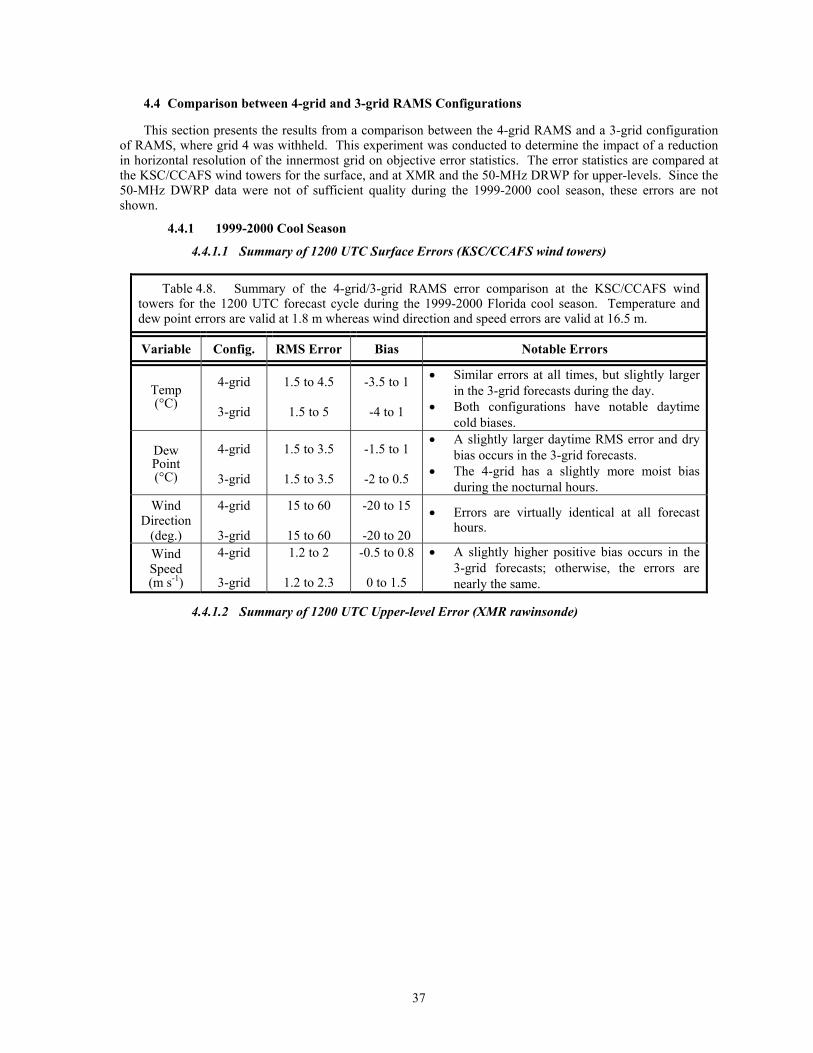
37

4.4 Comparison between 4-grid and 3-grid RAMS Configurations

This section presents the results from a comparison between the 4-grid RAMS and a 3-grid configuration of RAMS, where grid 4 was withheld. This experiment was conducted to determine the impact of a reduction in horizontal resolution of the innermost grid on objective error statistics. The error statistics are compared at the KSC/CCAFS wind towers for the surface, and at XMR and the 50-MHz DRWP for upper-levels. Since the 50-MHz DWRP data were not of sufficient quality during the 1999-2000 cool season, these errors are not shown.

4.4.1 1999-2000 Cool Season

4.4.1.1 Summary of 1200 UTC Surface Errors (KSC/CCAFS wind towers)

Table 4.8. Summary of the 4-grid/3-grid RAMS error comparison at the KSC/CCAFS wind towers for the 1200 UTC forecast cycle during the 1999-2000 Florida cool season. Temperature and dew point errors are valid at 1.8 m whereas wind direction and speed errors are valid at 16.5 m.

Variable Config. RMS Error Bias Notable Errors

Temp (°C)

4-grid

3-grid

1.5 to 4.5

1.5 to 5

-3.5 to 1

-4 to 1

• Similar errors at all times, but slightly larger in the 3-grid forecasts during the day.

• Both configurations have notable daytime cold biases.

Dew Point (°C)

4-grid

3-grid

1.5 to 3.5

1.5 to 3.5

-1.5 to 1

-2 to 0.5

• A slightly larger daytime RMS error and dry bias occurs in the 3-grid forecasts.

• The 4-grid has a slightly more moist bias during the nocturnal hours.

Wind Direction

(deg.)

4-grid

3-grid

15 to 60

15 to 60

-20 to 15

-20 to 20

• Errors are virtually identical at all forecast hours.

Wind Speed (m s-1)

4-grid

3-grid

1.2 to 2

1.2 to 2.3

-0.5 to 0.8

0 to 1.5

• A slightly higher positive bias occurs in the 3-grid forecasts; otherwise, the errors are nearly the same.

4.4.1.2 Summary of 1200 UTC Upper-level Error (XMR rawinsonde)

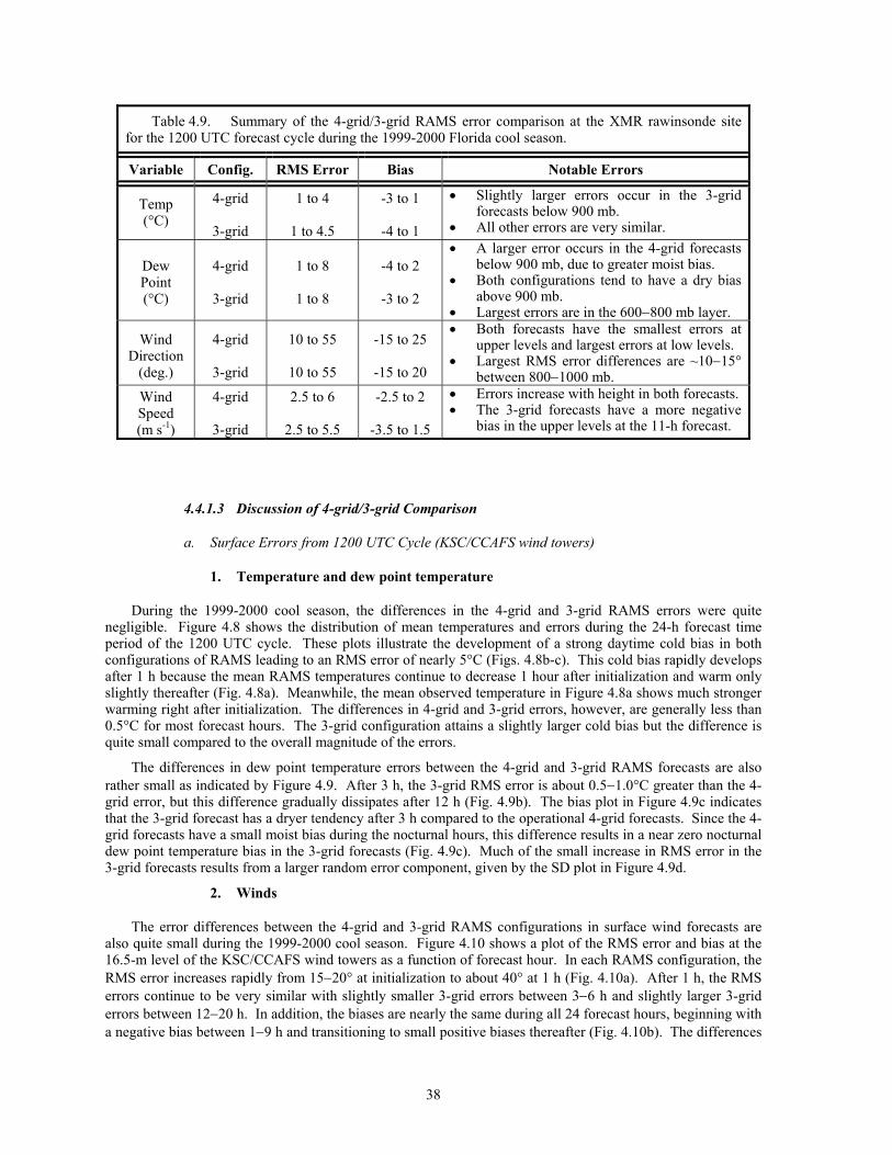
38

Table 4.9. Summary of the 4-grid/3-grid RAMS error comparison at the XMR rawinsonde site for the 1200 UTC forecast cycle during the 1999-2000 Florida cool season.

Variable Config. RMS Error Bias Notable Errors

Temp (°C)

4-grid

3-grid

1 to 4

1 to 4.5

-3 to 1

-4 to 1

• Slightly larger errors occur in the 3-grid forecasts below 900 mb.

• All other errors are very similar.

Dew Point (°C)

4-grid

3-grid

1 to 8

1 to 8

-4 to 2

-3 to 2

• A larger error occurs in the 4-grid forecasts below 900 mb, due to greater moist bias.

• Both configurations tend to have a dry bias above 900 mb.

• Largest errors are in the 600−800 mb layer.

Wind Direction

(deg.)

4-grid

3-grid

10 to 55

10 to 55

-15 to 25

-15 to 20

• Both forecasts have the smallest errors at upper levels and largest errors at low levels.

• Largest RMS error differences are ~10−15° between 800−1000 mb.

Wind Speed (m s-1)

4-grid

3-grid

2.5 to 6

2.5 to 5.5

-2.5 to 2

-3.5 to 1.5

• Errors increase with height in both forecasts. • The 3-grid forecasts have a more negative

bias in the upper levels at the 11-h forecast.

4.4.1.3 Discussion of 4-grid/3-grid Comparison

a. Surface Errors from 1200 UTC Cycle (KSC/CCAFS wind towers)

1. Temperature and dew point temperature

During the 1999-2000 cool season, the differences in the 4-grid and 3-grid RAMS errors were quite negligible. Figure 4.8 shows the distribution of mean temperatures and errors during the 24-h forecast time period of the 1200 UTC cycle. These plots illustrate the development of a strong daytime cold bias in both configurations of RAMS leading to an RMS error of nearly 5°C (Figs. 4.8b-c). This cold bias rapidly develops after 1 h because the mean RAMS temperatures continue to decrease 1 hour after initialization and warm only slightly thereafter (Fig. 4.8a). Meanwhile, the mean observed temperature in Figure 4.8a shows much stronger warming right after initialization. The differences in 4-grid and 3-grid errors, however, are generally less than 0.5°C for most forecast hours. The 3-grid configuration attains a slightly larger cold bias but the difference is quite small compared to the overall magnitude of the errors.

The differences in dew point temperature errors between the 4-grid and 3-grid RAMS forecasts are also rather small as indicated by Figure 4.9. After 3 h, the 3-grid RMS error is about 0.5−1.0°C greater than the 4-grid error, but this difference gradually dissipates after 12 h (Fig. 4.9b). The bias plot in Figure 4.9c indicates that the 3-grid forecast has a dryer tendency after 3 h compared to the operational 4-grid forecasts. Since the 4-grid forecasts have a small moist bias during the nocturnal hours, this difference results in a near zero nocturnal dew point temperature bias in the 3-grid forecasts (Fig. 4.9c). Much of the small increase in RMS error in the 3-grid forecasts results from a larger random error component, given by the SD plot in Figure 4.9d.

2. Winds

The error differences between the 4-grid and 3-grid RAMS configurations in surface wind forecasts are also quite small during the 1999-2000 cool season. Figure 4.10 shows a plot of the RMS error and bias at the 16.5-m level of the KSC/CCAFS wind towers as a function of forecast hour. In each RAMS configuration, the RMS error increases rapidly from 15−20° at initialization to about 40° at 1 h (Fig. 4.10a). After 1 h, the RMS errors continue to be very similar with slightly smaller 3-grid errors between 3−6 h and slightly larger 3-grid errors between 12−20 h. In addition, the biases are nearly the same during all 24 forecast hours, beginning with a negative bias between 1−9 h and transitioning to small positive biases thereafter (Fig. 4.10b). The differences

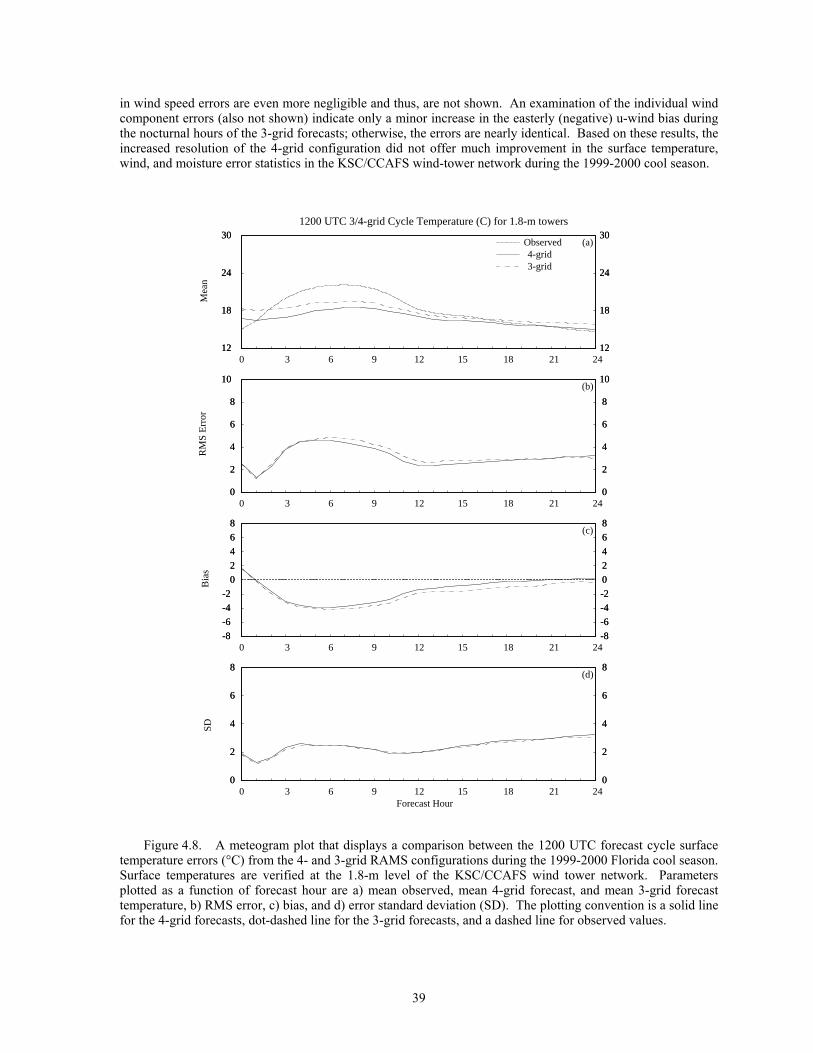
39

in wind speed errors are even more negligible and thus, are not shown. An examination of the individual wind component errors (also not shown) indicate only a minor increase in the easterly (negative) u-wind bias during the nocturnal hours of the 3-grid forecasts; otherwise, the errors are nearly identical. Based on these results, the increased resolution of the 4-grid configuration did not offer much improvement in the surface temperature, wind, and moisture error statistics in the KSC/CCAFS wind-tower network during the 1999-2000 cool season.

12

18

24

30

12

18

24

30

0

2

4

6

8

10

0

2

4

6

8

10

-8

-6

-4

-2

0

2

4

6

8

-8

-6

-4

-2

0

2

4

6

8

10/00 10/02 10/04 10/06 10/08 10/10 10/12 10/14 10/16 10/18 10/20 10/22 11/000

2

4

6

8

0

2

4

6

8

12

18

24

30

12

18

24

30

0

2

4

6

8

10

0

2

4

6

8

10

-8

-6

-4

-2

0

2

4

6

8

-8

-6

-4

-2

0

2

4

6

8

10/00 10/02 10/04 10/06 10/08 10/10 10/12 10/14 10/16 10/18 10/20 10/22 11/000

2

4

6

8

0

2

4

6

8

(a)Observed4-grid

(b)

(c)

(d)

Mea

nR

MS

Err

orB

ias

SD

0 3 6 9 12 15 18 21 24

0 3 6 9 12 15 18 21 24

0 3 6 9 12 15 18 21 24

0 3 6 9 12 15 18 21 24

Forecast Hour

1200 UTC 3/4-grid Cycle Temperature (C) for 1.8-m towers

3-grid

Figure 4.8. A meteogram plot that displays a comparison between the 1200 UTC forecast cycle surface

temperature errors (°C) from the 4- and 3-grid RAMS configurations during the 1999-2000 Florida cool season. Surface temperatures are verified at the 1.8-m level of the KSC/CCAFS wind tower network. Parameters plotted as a function of forecast hour are a) mean observed, mean 4-grid forecast, and mean 3-grid forecast temperature, b) RMS error, c) bias, and d) error standard deviation (SD). The plotting convention is a solid line for the 4-grid forecasts, dot-dashed line for the 3-grid forecasts, and a dashed line for observed values.

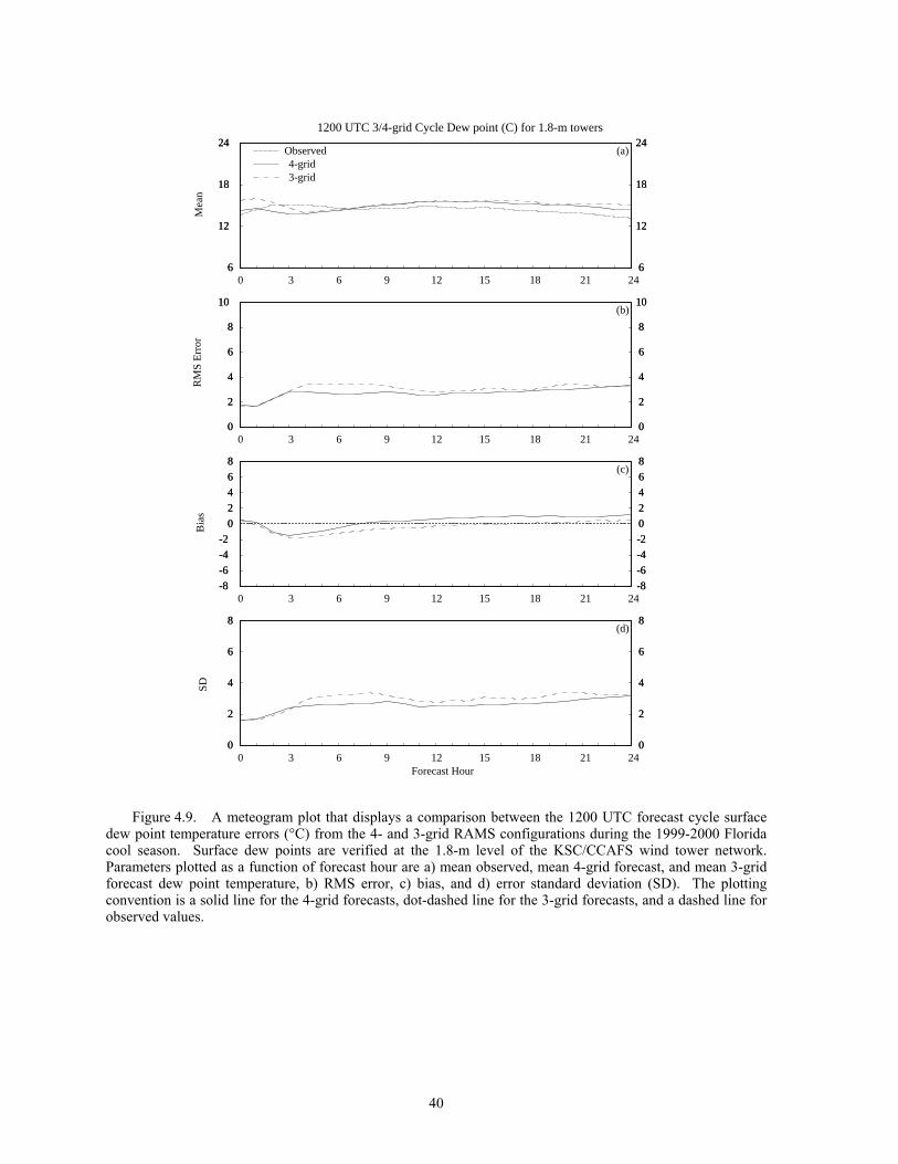
40

6

12

18

24

6

12

18

24

0

2

4

6

8

10

0

2

4

6

8

10

-8

-6

-4

-2

0

2

4

6

8

-8

-6

-4

-2

0

2

4

6

8

10/00 10/02 10/04 10/06 10/08 10/10 10/12 10/14 10/16 10/18 10/20 10/22 11/000

2

4

6

8

0

2

4

6

8

6

12

18

24

6

12

18

24

0

2

4

6

8

10

0

2

4

6

8

10

-8

-6

-4

-2

0

2

4

6

8

-8

-6

-4

-2

0

2

4

6

8

10/00 10/02 10/04 10/06 10/08 10/10 10/12 10/14 10/16 10/18 10/20 10/22 11/000

2

4

6

8

0

2

4

6

8

(a)Observed4-grid

(b)

(c)

(d)

Mea

nR

MS

Err

orB

ias

SD

0 3 6 9 12 15 18 21 24

0 3 6 9 12 15 18 21 24

0 3 6 9 12 15 18 21 24

0 3 6 9 12 15 18 21 24

Forecast Hour

1200 UTC 3/4-grid Cycle Dew point (C) for 1.8-m towers

3-grid

Figure 4.9. A meteogram plot that displays a comparison between the 1200 UTC forecast cycle surface

dew point temperature errors (°C) from the 4- and 3-grid RAMS configurations during the 1999-2000 Florida cool season. Surface dew points are verified at the 1.8-m level of the KSC/CCAFS wind tower network. Parameters plotted as a function of forecast hour are a) mean observed, mean 4-grid forecast, and mean 3-grid forecast dew point temperature, b) RMS error, c) bias, and d) error standard deviation (SD). The plotting convention is a solid line for the 4-grid forecasts, dot-dashed line for the 3-grid forecasts, and a dashed line for observed values.

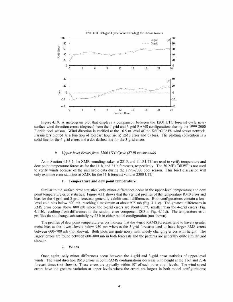
41

0

20

40

60

80

100

0

20

40

60

80

100

10/00 10/02 10/04 10/06 10/08 10/10 10/12 10/14 10/16 10/18 10/20 10/22 11/00-40

-20

0

20

40

-40

-20

0

20

40

0

20

40

60

80

100

0

20

40

60

80

100

10/00 10/02 10/04 10/06 10/08 10/10 10/12 10/14 10/16 10/18 10/20 10/22 11/00-40

-20

0

20

40

-40

-20

0

20

40

(a)

(b)

RM

S E

rror

Bia

s

0 3 6 9 12 15 18 21 24

0 3 6 9 12 15 18 21 24

Forecast Hour

1200 UTC 3/4-grid Cycle Wind Dir (deg) for 16.5-m towers

4-grid3-grid

Figure 4.10. A meteogram plot that displays a comparison between the 1200 UTC forecast cycle near-

surface wind direction errors (degrees) from the 4-grid and 3-grid RAMS configurations during the 1999-2000 Florida cool season. Wind direction is verified at the 16.5-m level of the KSC/CCAFS wind tower network. Parameters plotted as a function of forecast hour are a) RMS error and b) bias. The plotting convention is a solid line for the 4-grid errors and a dot-dashed line for the 3-grid errors.

b. Upper-level Errors from 1200 UTC Cycle (XMR rawinsonde)

As in Section 4.1.3.2, the XMR soundings taken at 2315, and 1115 UTC are used to verify temperature and dew point temperature forecasts for the 11-h, and 23-h forecasts, respectively. The 50-MHz DRWP is not used to verify winds because of the unreliable data during the 1999-2000 cool season. This brief discussion will only examine error statistics at XMR for the 11-h forecast valid at 2300 UTC.

1. Temperature and dew point temperature

Similar to the surface error statistics, only minor differences occur in the upper-level temperature and dew point temperature error statistics. Figure 4.11 shows that the vertical profiles of the temperature RMS error and bias for the 4-grid and 3-grid forecasts generally exhibit small differences. Both configurations contain a low-level cold bias below 600 mb, reaching a maximum at about 975 mb (Fig. 4.11c). The greatest differences in RMS error occur above 800 mb where the 3-grid errors are about 0.5°C smaller than the 4-grid errors (Fig. 4.11b), resulting from differences in the random error component (SD in Fig. 4.11d). The temperature error profiles do not change substantially by 23 h in either model configuration (not shown).

The profiles of dew point temperature errors indicate that the 4-grid RAMS forecasts tend to have a greater moist bias at the lowest levels below 950 mb whereas the 3-grid forecasts tend to have larger RMS errors between 600−700 mb (not shown). Both plots are quite noisy with widely changing errors with height. The largest errors are found between 600−800 mb in both forecasts and the patterns are generally quite similar (not shown).

2. Winds

Once again, only minor differences occur between the 4-grid and 3-grid error statistics of upper-level winds. The wind direction RMS errors in both RAMS configurations decrease with height at the 11-h and 23-h forecast times (not shown). These errors are typically within 10° of each other at all levels. The wind speed errors have the greatest variation at upper levels where the errors are largest in both model configurations;

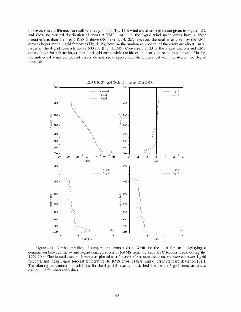
42

however, these differences are still relatively minor. The 11-h wind speed error plots are given in Figure 4.12 and show the vertical distribution of errors at XMR. At 11 h, the 3-grid wind speed errors have a larger negative bias than the 4-grid RAMS above 600 mb (Fig. 4.12c); however, the total error given by the RMS error is larger in the 4-grid forecasts (Fig. 4.12b) because the random component of the errors are about 1 m s-1 larger in the 4-grid forecasts above 500 mb (Fig. 4.12d). Conversely at 23 h, the 3-grid random and RMS errors above 600 mb are larger than the 4-grid errors while the biases are nearly the same (not shown). Finally, the individual wind component errors do not show appreciable differences between the 4-grid and 3-grid forecasts.

-30 -20 -10 0 10 20 30

300

400

500

600

700

800

900

1000

-30 -20 -10 0 10 20 30

300

400

500

600

700

800

900

1000

-30 -20 -10 0 10 20 30

300

400

500

600

700

800

900

1000

0 2 4 6

300

400

500

600

700

800

900

1000

0 2 4 6

300

400

500

600

700

800

900

1000

0 2 4 6

300

400

500

600

700

800

900

1000

0 2 4 6

300

400

500

600

700

800

900

1000

-6 -4 -2 0 2 4 6

300

400

500

600

700

800

900

1000

-6 -4 -2 0 2 4 6

300

400

500

600

700

800

900

1000

Observed4-grid

Mean

(a)

RMS Error

(b)

SD

(d)

Bias

(c)

Pres

sure

(m

b)

Pres

sure

(m

b)

Pres

sure

(m

b)

Pres

sure

(m

b)

1200 UTC 3/4-grid Cycle 11-h Temp (C) at XMR

3-grid

4-grid3-grid

4-grid3-grid

4-grid3-grid

Figure 4.11. Vertical profiles of temperature errors (°C) at XMR for the 11-h forecast, displaying a

comparison between the 4- and 3-grid configurations of RAMS from the 1200 UTC forecast cycle during the 1999-2000 Florida cool season. Parameters plotted as a function of pressure are a) mean observed, mean 4-grid forecast, and mean 3-grid forecast temperature, b) RMS error, c) bias, and d) error standard deviation (SD). The plotting convention is a solid line for the 4-grid forecasts, dot-dashed line for the 3-grid forecasts, and a dashed line for observed values.

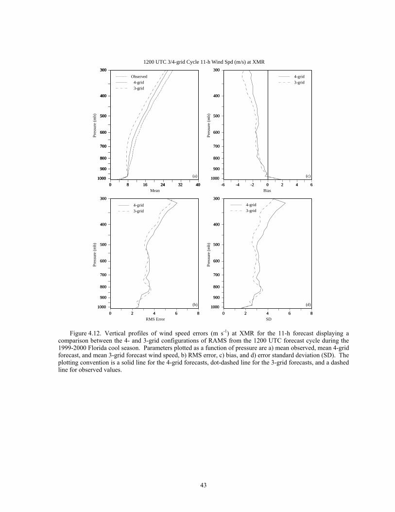
43

0 8 16 24 32 40

300

400

500

600

700

800

900

1000

0 8 16 24 32 40

300

400

500

600

700

800

900

1000

0 8 16 24 32 40

300

400

500

600

700

800

900

1000

0 2 4 6 8

300

400

500

600

700

800

900

1000

0 2 4 6 8

300

400

500

600

700

800

900

1000

0 2 4 6 8

300

400

500

600

700

800

900

1000

0 2 4 6 8

300

400

500

600

700

800

900

1000

-6 -4 -2 0 2 4 6

300

400

500

600

700

800

900

1000

-6 -4 -2 0 2 4 6

300

400

500

600

700

800

900

1000

Observed4-grid

Mean

(a)

RMS Error

(b)

SD

(d)

Bias

(c)

Pres

sure

(m

b)

Pres

sure

(m

b)

Pres

sure

(m

b)

Pres

sure

(m

b)

1200 UTC 3/4-grid Cycle 11-h Wind Spd (m/s) at XMR

3-grid

4-grid3-grid

4-grid3-grid

4-grid3-grid

Figure 4.12. Vertical profiles of wind speed errors (m s-1) at XMR for the 11-h forecast displaying a

comparison between the 4- and 3-grid configurations of RAMS from the 1200 UTC forecast cycle during the 1999-2000 Florida cool season. Parameters plotted as a function of pressure are a) mean observed, mean 4-grid forecast, and mean 3-grid forecast wind speed, b) RMS error, c) bias, and d) error standard deviation (SD). The plotting convention is a solid line for the 4-grid forecasts, dot-dashed line for the 3-grid forecasts, and a dashed line for observed values.

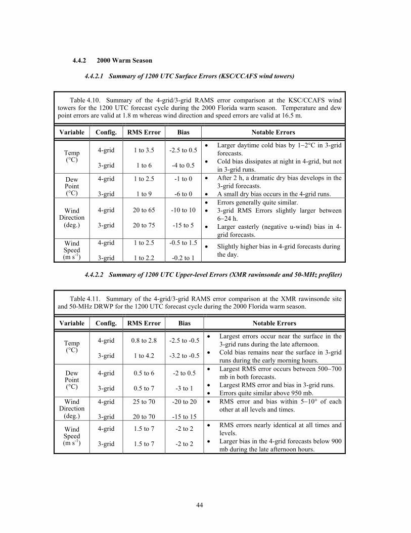
44

4.4.2 2000 Warm Season

4.4.2.1 Summary of 1200 UTC Surface Errors (KSC/CCAFS wind towers)

Table 4.10. Summary of the 4-grid/3-grid RAMS error comparison at the KSC/CCAFS wind towers for the 1200 UTC forecast cycle during the 2000 Florida warm season. Temperature and dew point errors are valid at 1.8 m whereas wind direction and speed errors are valid at 16.5 m.

Variable Config. RMS Error Bias Notable Errors

Temp (°C)

4-grid

3-grid

1 to 3.5

1 to 6

-2.5 to 0.5

-4 to 0.5

• Larger daytime cold bias by 1−2°C in 3-grid forecasts.

• Cold bias dissipates at night in 4-grid, but not in 3-grid runs.

Dew Point (°C)

4-grid

3-grid

1 to 2.5

1 to 9

-1 to 0

-6 to 0

• After 2 h, a dramatic dry bias develops in the 3-grid forecasts.

• A small dry bias occurs in the 4-grid runs.

Wind Direction

(deg.)

4-grid

3-grid

20 to 65

20 to 75

-10 to 10

-15 to 5

• Errors generally quite similar. • 3-grid RMS Errors slightly larger between

6−24 h. • Larger easterly (negative u-wind) bias in 4-

grid forecasts. Wind Speed (m s-1)

4-grid

3-grid

1 to 2.5

1 to 2.2

-0.5 to 1.5

-0.2 to 1

• Slightly higher bias in 4-grid forecasts during the day.

4.4.2.2 Summary of 1200 UTC Upper-level Errors (XMR rawinsonde and 50-MHz profiler)

Table 4.11. Summary of the 4-grid/3-grid RAMS error comparison at the XMR rawinsonde site and 50-MHz DRWP for the 1200 UTC forecast cycle during the 2000 Florida warm season.

Variable Config. RMS Error Bias Notable Errors

Temp (°C)

4-grid

3-grid

0.8 to 2.8

1 to 4.2

-2.5 to -0.5

-3.2 to -0.5

• Largest errors occur near the surface in the 3-grid runs during the late afternoon.

• Cold bias remains near the surface in 3-grid runs during the early morning hours.

Dew Point (°C)

4-grid

3-grid

0.5 to 6

0.5 to 7

-2 to 0.5

-3 to 1

• Largest RMS error occurs between 500−700 mb in both forecasts.

• Largest RMS error and bias in 3-grid runs. • Errors quite similar above 950 mb.

Wind Direction

(deg.)

4-grid

3-grid

25 to 70

20 to 70

-20 to 20

-15 to 15

• RMS error and bias within 5−10° of each other at all levels and times.

Wind Speed (m s-1)

4-grid

3-grid

1.5 to 7

1.5 to 7

-2 to 2

-2 to 2

• RMS errors nearly identical at all times and levels.

• Larger bias in the 4-grid forecasts below 900 mb during the late afternoon hours.

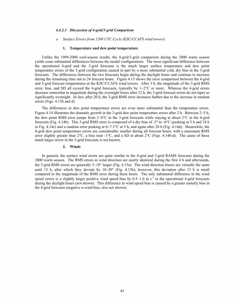
45

4.4.2.3 Discussion of 4-grid/3-grid Comparison

a. Surface Errors from 1200 UTC Cycle (KSC/CCAFS wind towers)

1. Temperature and dew point temperature

Unlike the 1999-2000 cool-season results, the 4-grid/3-grid comparison during the 2000 warm season yields some substantial differences between the model configurations. The most significant difference between the operational 4-grid and the 3-grid forecasts is the much larger surface temperature and dew point temperature errors of the 3-grid configuration caused in part by a more substantial cold, dry bias in the 3-grid forecasts. The differences between the two forecasts begin during the daylight hours and continue to increase during the remaining time out to 24 forecast hours. Figure 4.13 shows the error comparison between the 4-grid and 3-grid forecast temperatures at the KSC/CCAFS wind towers. After 3 h, the magnitude of the 3-grid RMS error, bias, and SD all exceed the 4-grid forecasts, typically by 1−2°C or more. Whereas the 4-grid errors decrease somewhat in magnitude during the overnight hours after 12 h, the 3-grid forecast errors do not taper as significantly overnight. In fact, after 20 h, the 3-grid RMS error increases further due to the increase in random errors (Figs. 4.13b and d).

The differences in dew point temperature errors are even more substantial than the temperature errors. Figure 4.14 illustrates the dramatic growth in the 3-grid dew point temperature errors after 2 h. Between 2−5 h, the dew point RMS error jumps from 2−8°C in the 3-grid forecasts while staying at about 2°C in the 4-grid forecasts (Fig. 4.14b). This 3-grid RMS error is composed of a dry bias of -5° to -6°C (peaking at 5 h and 24 h in Fig. 4.14c) and a random error peaking at 6−7.5°C at 5 h, and again after 20 h (Fig. 4.14d). Meanwhile, the 4-grid dew point temperature errors are considerably smaller during all forecast hours, with a maximum RMS error slightly greater than 2°C, a bias near -1°C, and a SD at about 2°C (Figs. 4.14b-d). The cause of these much larger errors in the 3-grid forecasts is not known.

2. Winds

In general, the surface wind errors are quite similar in the 4-grid and 3-grid RAMS forecasts during the 2000 warm season. The RMS errors in wind direction are nearly identical during the first 4 h and afterwards, the 3-grid RMS errors are generally 5−10° larger (Fig. 4.15a). The wind direction biases are virtually the same until 13 h, after which they deviate by 10−20° (Fig. 4.15b); however, this deviation after 13 h is small compared to the magnitude of the RMS error during these hours. The only substantial difference in the wind speed errors is a slightly larger positive wind speed bias by 0.5−1.0 m s-1 in the operational 4-grid forecasts during the daylight hours (not shown). This difference in wind speed bias is caused by a greater easterly bias in the 4-grid forecasts (negative u-wind bias, also not shown).

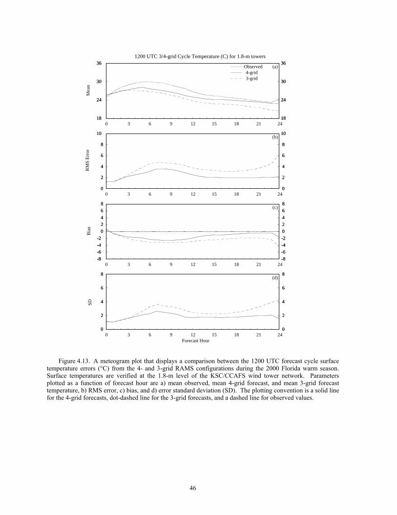
46

18

24

30

36

18

24

30

36

0

2

4

6

8

10

0

2

4

6

8

10

-8

-6

-4

-2

0

2

4

6

8

-8

-6

-4

-2

0

2

4

6

8

10/00 10/02 10/04 10/06 10/08 10/10 10/12 10/14 10/16 10/18 10/20 10/22 11/000

2

4

6

8

0

2

4

6

8

18

24

30

36

18

24

30

36

0

2

4

6

8

10

0

2

4

6

8

10

-8

-6

-4

-2

0

2

4

6

8

-8

-6

-4

-2

0

2

4

6

8

10/00 10/02 10/04 10/06 10/08 10/10 10/12 10/14 10/16 10/18 10/20 10/22 11/000

2

4

6

8

0

2

4

6

8

(a)Observed4-grid

(b)

(c)

(d)

Mea

nR

MS

Err

orB

ias

SD

0 3 6 9 12 15 18 21 24

0 3 6 9 12 15 18 21 24

0 3 6 9 12 15 18 21 24

0 3 6 9 12 15 18 21 24

Forecast Hour

1200 UTC 3/4-grid Cycle Temperature (C) for 1.8-m towers

3-grid

Figure 4.13. A meteogram plot that displays a comparison between the 1200 UTC forecast cycle surface

temperature errors (°C) from the 4- and 3-grid RAMS configurations during the 2000 Florida warm season. Surface temperatures are verified at the 1.8-m level of the KSC/CCAFS wind tower network. Parameters plotted as a function of forecast hour are a) mean observed, mean 4-grid forecast, and mean 3-grid forecast temperature, b) RMS error, c) bias, and d) error standard deviation (SD). The plotting convention is a solid line for the 4-grid forecasts, dot-dashed line for the 3-grid forecasts, and a dashed line for observed values.

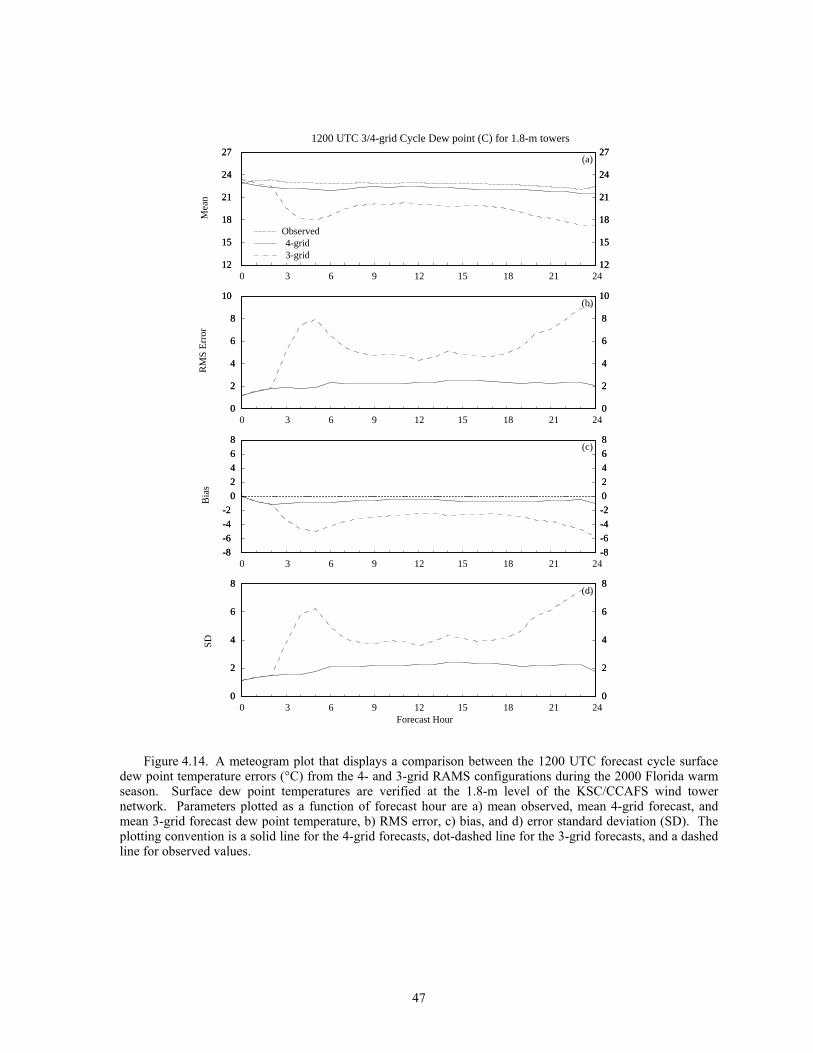
47

12

15

18

21

24

27

12

15

18

21

24

27

0

2

4

6

8

10

0

2

4

6

8

10

-8

-6

-4

-2

0

2

4

6

8

-8

-6

-4

-2

0

2

4

6

8

10/00 10/02 10/04 10/06 10/08 10/10 10/12 10/14 10/16 10/18 10/20 10/22 11/000

2

4

6

8

0

2

4

6

8

12

15

18

21

24

27

12

15

18

21

24

27

0

2

4

6

8

10

0

2

4

6

8

10

-8

-6

-4

-2

0

2

4

6

8

-8

-6

-4

-2

0

2

4

6

8

10/00 10/02 10/04 10/06 10/08 10/10 10/12 10/14 10/16 10/18 10/20 10/22 11/000

2

4

6

8

0

2

4

6

8

(a)

Observed4-grid

(b)

(c)

(d)

Mea

nR

MS

Err

orB

ias

SD

0 3 6 9 12 15 18 21 24

0 3 6 9 12 15 18 21 24

0 3 6 9 12 15 18 21 24

0 3 6 9 12 15 18 21 24

Forecast Hour

1200 UTC 3/4-grid Cycle Dew point (C) for 1.8-m towers

3-grid

Figure 4.14. A meteogram plot that displays a comparison between the 1200 UTC forecast cycle surface

dew point temperature errors (°C) from the 4- and 3-grid RAMS configurations during the 2000 Florida warm season. Surface dew point temperatures are verified at the 1.8-m level of the KSC/CCAFS wind tower network. Parameters plotted as a function of forecast hour are a) mean observed, mean 4-grid forecast, and mean 3-grid forecast dew point temperature, b) RMS error, c) bias, and d) error standard deviation (SD). The plotting convention is a solid line for the 4-grid forecasts, dot-dashed line for the 3-grid forecasts, and a dashed line for observed values.

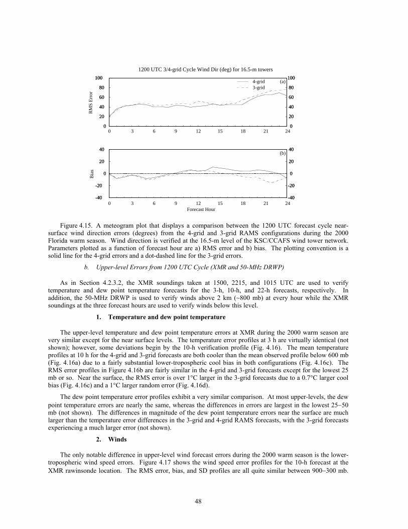
48

0

20

40

60

80

100

0

20

40

60

80

100

10/00 10/02 10/04 10/06 10/08 10/10 10/12 10/14 10/16 10/18 10/20 10/22 11/00-40

-20

0

20

40

-40

-20

0

20

40

0

20

40

60

80

100

0

20

40

60

80

100

10/00 10/02 10/04 10/06 10/08 10/10 10/12 10/14 10/16 10/18 10/20 10/22 11/00-40

-20

0

20

40

-40

-20

0

20

40

(a)

(b)

RM

S E

rror

Bia

s

0 3 6 9 12 15 18 21 24

0 3 6 9 12 15 18 21 24

Forecast Hour

1200 UTC 3/4-grid Cycle Wind Dir (deg) for 16.5-m towers

4-grid3-grid

Figure 4.15. A meteogram plot that displays a comparison between the 1200 UTC forecast cycle near-

surface wind direction errors (degrees) from the 4-grid and 3-grid RAMS configurations during the 2000 Florida warm season. Wind direction is verified at the 16.5-m level of the KSC/CCAFS wind tower network. Parameters plotted as a function of forecast hour are a) RMS error and b) bias. The plotting convention is a solid line for the 4-grid errors and a dot-dashed line for the 3-grid errors.

b. Upper-level Errors from 1200 UTC Cycle (XMR and 50-MHz DRWP)

As in Section 4.2.3.2, the XMR soundings taken at 1500, 2215, and 1015 UTC are used to verify temperature and dew point temperature forecasts for the 3-h, 10-h, and 22-h forecasts, respectively. In addition, the 50-MHz DRWP is used to verify winds above 2 km (~800 mb) at every hour while the XMR soundings at the three forecast hours are used to verify winds below this level.

1. Temperature and dew point temperature

The upper-level temperature and dew point temperature errors at XMR during the 2000 warm season are very similar except for the near surface levels. The temperature error profiles at 3 h are virtually identical (not shown); however, some deviations begin by the 10-h verification profile (Fig. 4.16). The mean temperature profiles at 10 h for the 4-grid and 3-grid forecasts are both cooler than the mean observed profile below 600 mb (Fig. 4.16a) due to a fairly substantial lower-tropospheric cool bias in both configurations (Fig. 4.16c). The RMS error profiles in Figure 4.16b are fairly similar in the 4-grid and 3-grid forecasts except for the lowest 25 mb or so. Near the surface, the RMS error is over 1°C larger in the 3-grid forecasts due to a 0.7°C larger cool bias (Fig. 4.16c) and a 1°C larger random error (Fig. 4.16d).

The dew point temperature error profiles exhibit a very similar comparison. At most upper-levels, the dew point temperature errors are nearly the same, whereas the differences in errors are largest in the lowest 25−50 mb (not shown). The differences in magnitude of the dew point temperature errors near the surface are much larger than the temperature error differences in the 3-grid and 4-grid RAMS forecasts, with the 3-grid forecasts experiencing a much larger error (not shown).

2. Winds

The only notable difference in upper-level wind forecast errors during the 2000 warm season is the lower-tropospheric wind speed errors. Figure 4.17 shows the wind speed error profiles for the 10-h forecast at the XMR rawinsonde location. The RMS error, bias, and SD profiles are all quite similar between 900−300 mb.

49

The only substantial differences in errors occurs below 900 mb where a larger RMS error by about 1 m s-1 is found in the operational 4-grid forecasts (Fig. 4.17b). This difference in RMS error is almost entirely attributed to a larger positive wind speed bias in the 4-grid forecasts compared to the 3-grid configuration (Fig. 4.17c).

The upper-level wind direction errors are within 0−10° of each other at all times and levels for both the 50-MHz DRWP and the XMR rawinsonde (not shown). Also not shown are the individual wind component errors, which have only minor differences throughout the troposphere.

4.4.3 Summary of 4-grid/3-grid Error Comparison

The collective results from the 4-grid/3-grid comparison during the 1999-2000 cool, and 1999 and 2000 warm seasons suggest the following about the RAMS model in east-central Florida:

• Running a higher-resolution configuration of RAMS results in a significant improvement in the surface temperature and moisture error statistics during the warm season, but not during the cool season.

• The error comparison does not yield a noticeable improvement in the surface and upper-level wind error statistics during both seasons.

• During the warm season, the higher resolution configuration of RAMS tends to over predict wind speeds at the surface and lower levels of the atmosphere.

Additional subjective evaluations in Section 5 will help to illustrate the total benefit of running the higher resolution, operational configuration of RAMS, particularly with respect to sea-breeze forecasts within the KSC/CCAFS wind-tower network.

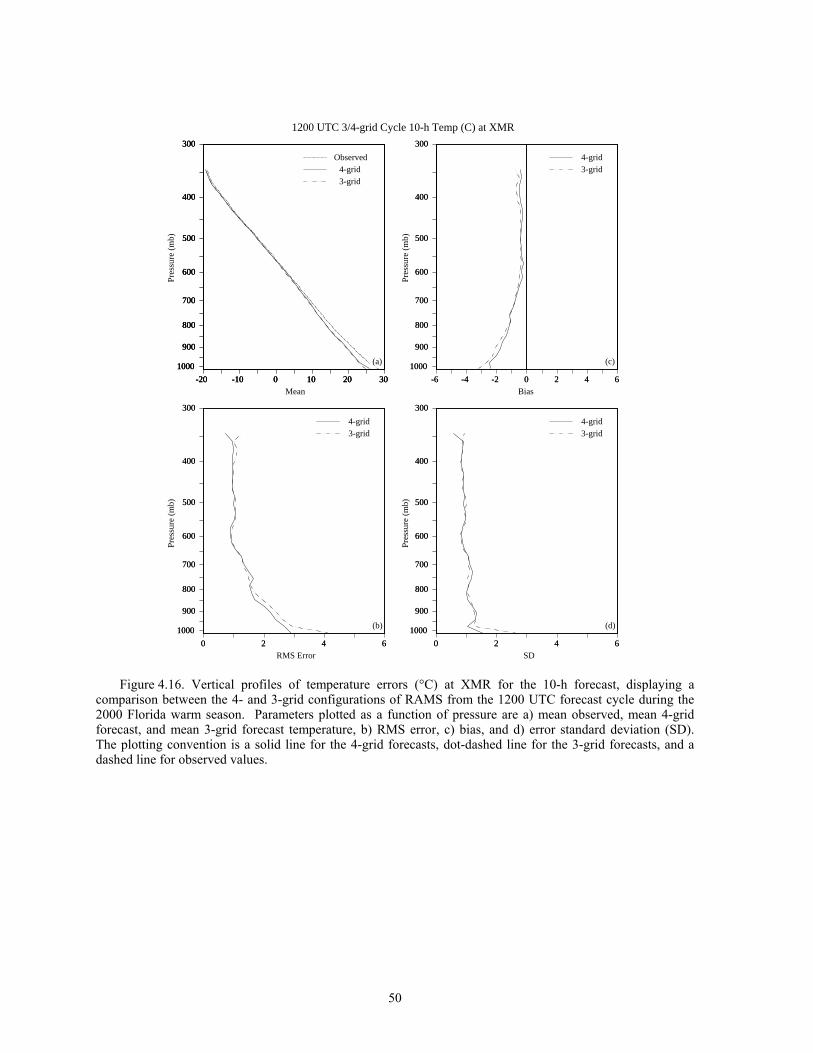
50

-20 -10 0 10 20 30

300

400

500

600

700

800

900

1000

-20 -10 0 10 20 30

300

400

500

600

700

800

900

1000

-20 -10 0 10 20 30

300

400

500

600

700

800

900

1000

0 2 4 6

300

400

500

600

700

800

900

1000

0 2 4 6

300

400

500

600

700

800

900

1000

0 2 4 6

300

400

500

600

700

800

900

1000

0 2 4 6

300

400

500

600

700

800

900

1000

-6 -4 -2 0 2 4 6

300

400

500

600

700

800

900

1000

-6 -4 -2 0 2 4 6

300

400

500

600

700

800

900

1000

Observed4-grid

Mean

(a)

RMS Error

(b)

SD

(d)

Bias

(c)

Pres

sure

(m

b)

Pres

sure

(m

b)

Pres

sure

(m

b)

Pres

sure

(m

b)

1200 UTC 3/4-grid Cycle 10-h Temp (C) at XMR

3-grid

4-grid3-grid

4-grid3-grid

4-grid3-grid

Figure 4.16. Vertical profiles of temperature errors (°C) at XMR for the 10-h forecast, displaying a

comparison between the 4- and 3-grid configurations of RAMS from the 1200 UTC forecast cycle during the 2000 Florida warm season. Parameters plotted as a function of pressure are a) mean observed, mean 4-grid forecast, and mean 3-grid forecast temperature, b) RMS error, c) bias, and d) error standard deviation (SD). The plotting convention is a solid line for the 4-grid forecasts, dot-dashed line for the 3-grid forecasts, and a dashed line for observed values.

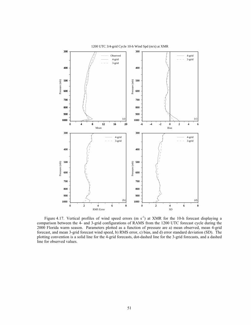
51

0 4 8 12 16 20

300

400

500

600

700

800

900

1000

0 4 8 12 16 20

300

400

500

600

700

800

900

1000

0 4 8 12 16 20

300

400

500

600

700

800

900

1000

0 2 4 6 8

300

400

500

600

700

800

900

1000

0 2 4 6 8

300

400

500

600

700

800

900

1000

0 2 4 6 8

300

400

500

600

700

800

900

1000

0 2 4 6 8

300

400

500

600

700

800

900

1000

-6 -4 -2 0 2 4 6

300

400

500

600

700

800

900

1000

-6 -4 -2 0 2 4 6

300

400

500

600

700

800

900

1000

Observed4-grid

Mean

(a)

RMS Error

(b)

SD

(d)

Bias

(c)

Pres

sure

(m

b)

Pres

sure

(m

b)

Pres

sure

(m

b)

Pres

sure

(m

b)

1200 UTC 3/4-grid Cycle 10-h Wind Spd (m/s) at XMR

3-grid

4-grid3-grid

4-grid3-grid

4-grid3-grid

Figure 4.17. Vertical profiles of wind speed errors (m s-1) at XMR for the 10-h forecast displaying a

comparison between the 4- and 3-grid configurations of RAMS from the 1200 UTC forecast cycle during the 2000 Florida warm season. Parameters plotted as a function of pressure are a) mean observed, mean 4-grid forecast, and mean 3-grid forecast wind speed, b) RMS error, c) bias, and d) error standard deviation (SD). The plotting convention is a solid line for the 4-grid forecasts, dot-dashed line for the 3-grid forecasts, and a dashed line for observed values.

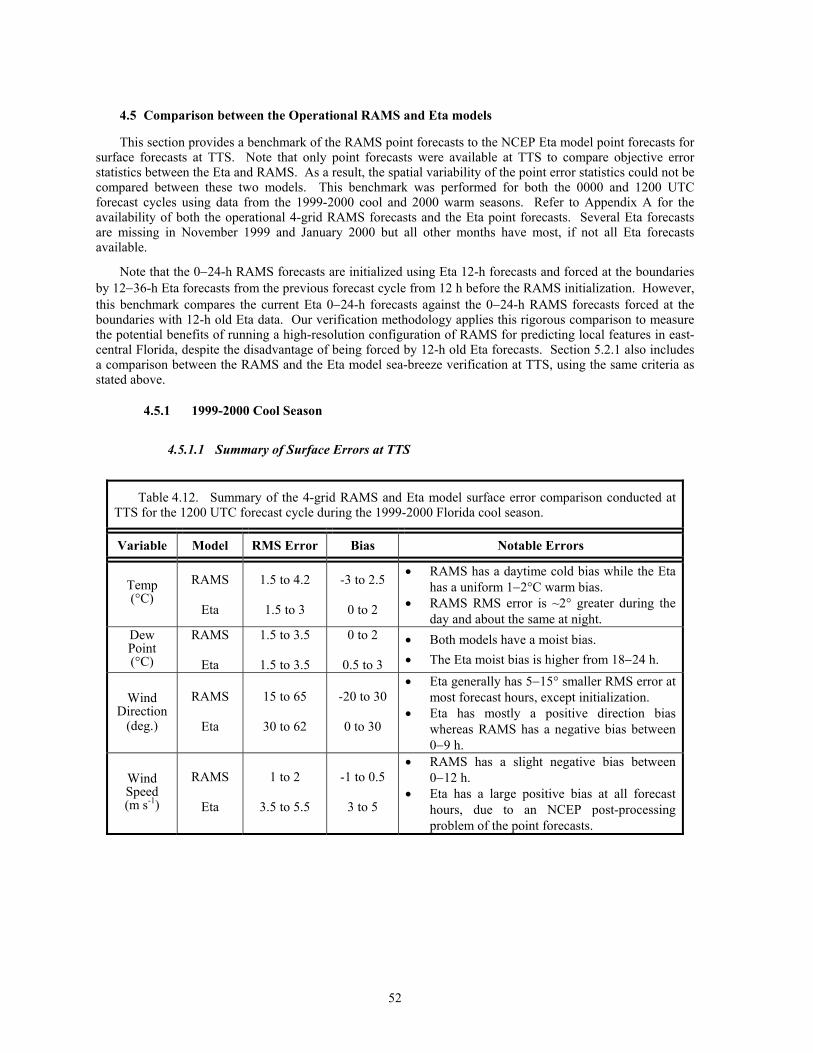
52

4.5 Comparison between the Operational RAMS and Eta models

This section provides a benchmark of the RAMS point forecasts to the NCEP Eta model point forecasts for surface forecasts at TTS. Note that only point forecasts were available at TTS to compare objective error statistics between the Eta and RAMS. As a result, the spatial variability of the point error statistics could not be compared between these two models. This benchmark was performed for both the 0000 and 1200 UTC forecast cycles using data from the 1999-2000 cool and 2000 warm seasons. Refer to Appendix A for the availability of both the operational 4-grid RAMS forecasts and the Eta point forecasts. Several Eta forecasts are missing in November 1999 and January 2000 but all other months have most, if not all Eta forecasts available.

Note that the 0−24-h RAMS forecasts are initialized using Eta 12-h forecasts and forced at the boundaries by 12−36-h Eta forecasts from the previous forecast cycle from 12 h before the RAMS initialization. However, this benchmark compares the current Eta 0−24-h forecasts against the 0−24-h RAMS forecasts forced at the boundaries with 12-h old Eta data. Our verification methodology applies this rigorous comparison to measure the potential benefits of running a high-resolution configuration of RAMS for predicting local features in east-central Florida, despite the disadvantage of being forced by 12-h old Eta forecasts. Section 5.2.1 also includes a comparison between the RAMS and the Eta model sea-breeze verification at TTS, using the same criteria as stated above.

4.5.1 1999-2000 Cool Season

4.5.1.1 Summary of Surface Errors at TTS

Table 4.12. Summary of the 4-grid RAMS and Eta model surface error comparison conducted at TTS for the 1200 UTC forecast cycle during the 1999-2000 Florida cool season.

Variable Model RMS Error Bias Notable Errors

Temp (°C)

RAMS

Eta

1.5 to 4.2

1.5 to 3

-3 to 2.5

0 to 2

• RAMS has a daytime cold bias while the Eta has a uniform 1−2°C warm bias.

• RAMS RMS error is ~2° greater during the day and about the same at night.

Dew Point (°C)

RAMS

Eta

1.5 to 3.5

1.5 to 3.5

0 to 2

0.5 to 3

• Both models have a moist bias. • The Eta moist bias is higher from 18−24 h.

Wind Direction

(deg.)

RAMS

Eta

15 to 65

30 to 62

-20 to 30

0 to 30

• Eta generally has 5−15° smaller RMS error at most forecast hours, except initialization.

• Eta has mostly a positive direction bias whereas RAMS has a negative bias between 0−9 h.

Wind Speed (m s-1)

RAMS

Eta

1 to 2

3.5 to 5.5

-1 to 0.5

3 to 5

• RAMS has a slight negative bias between 0−12 h.

• Eta has a large positive bias at all forecast hours, due to an NCEP post-processing problem of the point forecasts.

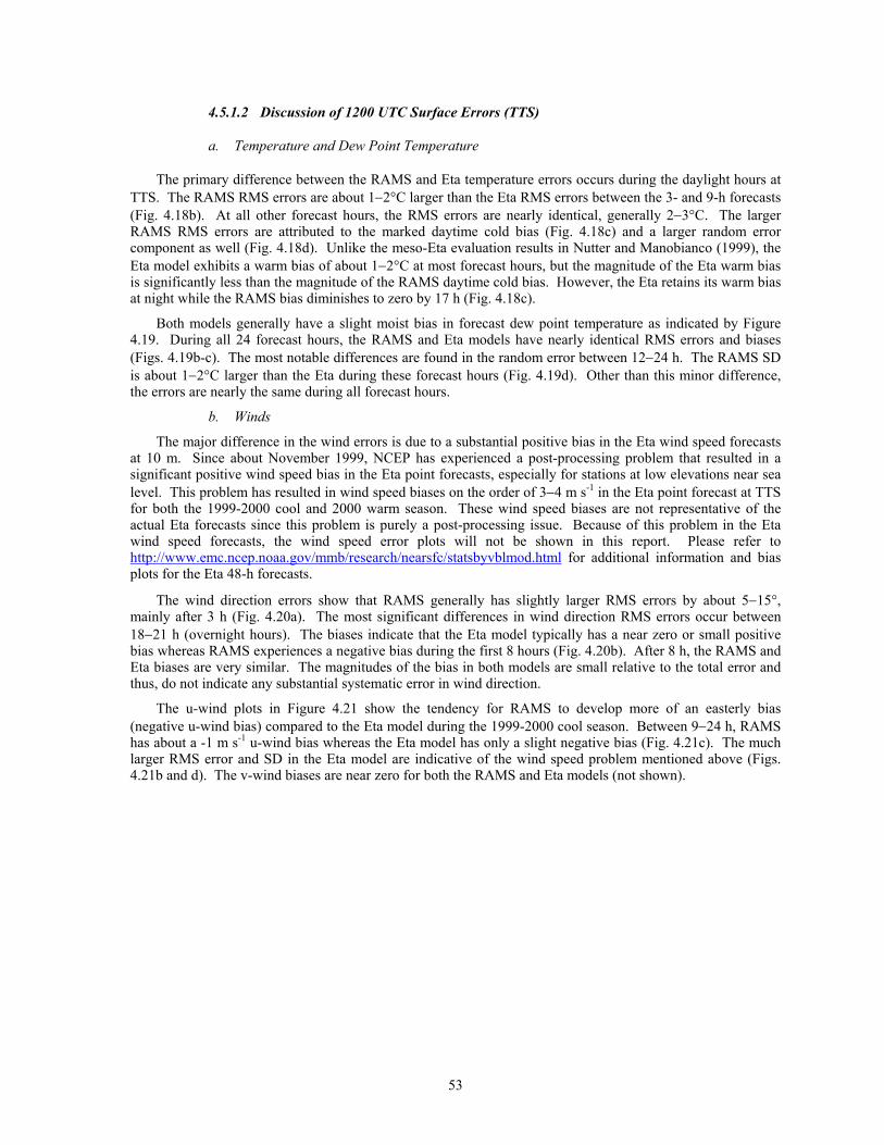
53

4.5.1.2 Discussion of 1200 UTC Surface Errors (TTS)

a. Temperature and Dew Point Temperature

The primary difference between the RAMS and Eta temperature errors occurs during the daylight hours at TTS. The RAMS RMS errors are about 1−2°C larger than the Eta RMS errors between the 3- and 9-h forecasts (Fig. 4.18b). At all other forecast hours, the RMS errors are nearly identical, generally 2−3°C. The larger RAMS RMS errors are attributed to the marked daytime cold bias (Fig. 4.18c) and a larger random error component as well (Fig. 4.18d). Unlike the meso-Eta evaluation results in Nutter and Manobianco (1999), the Eta model exhibits a warm bias of about 1−2°C at most forecast hours, but the magnitude of the Eta warm bias is significantly less than the magnitude of the RAMS daytime cold bias. However, the Eta retains its warm bias at night while the RAMS bias diminishes to zero by 17 h (Fig. 4.18c).

Both models generally have a slight moist bias in forecast dew point temperature as indicated by Figure 4.19. During all 24 forecast hours, the RAMS and Eta models have nearly identical RMS errors and biases (Figs. 4.19b-c). The most notable differences are found in the random error between 12−24 h. The RAMS SD is about 1−2°C larger than the Eta during these forecast hours (Fig. 4.19d). Other than this minor difference, the errors are nearly the same during all forecast hours.

b. Winds

The major difference in the wind errors is due to a substantial positive bias in the Eta wind speed forecasts at 10 m. Since about November 1999, NCEP has experienced a post-processing problem that resulted in a significant positive wind speed bias in the Eta point forecasts, especially for stations at low elevations near sea level. This problem has resulted in wind speed biases on the order of 3−4 m s-1 in the Eta point forecast at TTS for both the 1999-2000 cool and 2000 warm season. These wind speed biases are not representative of the actual Eta forecasts since this problem is purely a post-processing issue. Because of this problem in the Eta wind speed forecasts, the wind speed error plots will not be shown in this report. Please refer to http://www.emc.ncep.noaa.gov/mmb/research/nearsfc/statsbyvblmod.html for additional information and bias plots for the Eta 48-h forecasts.

The wind direction errors show that RAMS generally has slightly larger RMS errors by about 5−15°, mainly after 3 h (Fig. 4.20a). The most significant differences in wind direction RMS errors occur between 18−21 h (overnight hours). The biases indicate that the Eta model typically has a near zero or small positive bias whereas RAMS experiences a negative bias during the first 8 hours (Fig. 4.20b). After 8 h, the RAMS and Eta biases are very similar. The magnitudes of the bias in both models are small relative to the total error and thus, do not indicate any substantial systematic error in wind direction.

The u-wind plots in Figure 4.21 show the tendency for RAMS to develop more of an easterly bias (negative u-wind bias) compared to the Eta model during the 1999-2000 cool season. Between 9−24 h, RAMS has about a -1 m s-1 u-wind bias whereas the Eta model has only a slight negative bias (Fig. 4.21c). The much larger RMS error and SD in the Eta model are indicative of the wind speed problem mentioned above (Figs. 4.21b and d). The v-wind biases are near zero for both the RAMS and Eta models (not shown).

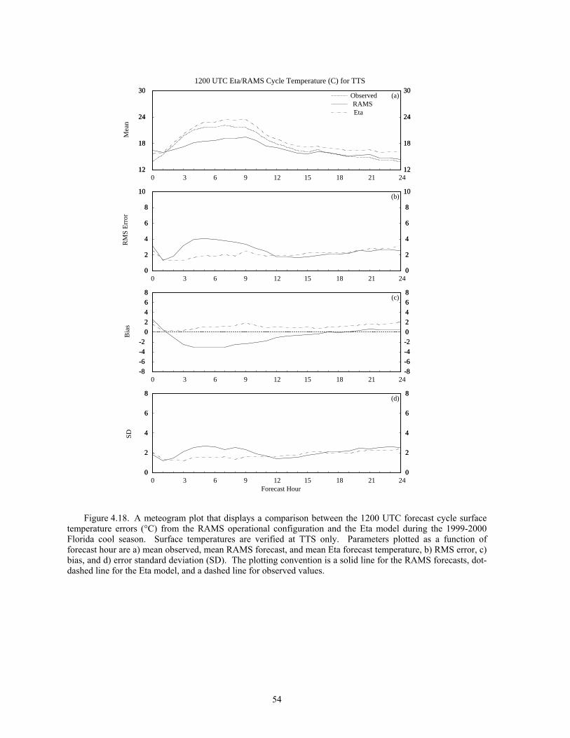
54

12

18

24

30

12

18

24

30

0

2

4

6

8

10

0

2

4

6

8

10

-8

-6

-4

-2

0

2

4

6

8

-8

-6

-4

-2

0

2

4

6

8

10/00 10/02 10/04 10/06 10/08 10/10 10/12 10/14 10/16 10/18 10/20 10/22 11/000

2

4

6

8

0

2

4

6

8

12

18

24

30

12

18

24

30

0

2

4

6

8

10

0

2

4

6

8

10

-8

-6

-4

-2

0

2

4

6

8

-8

-6

-4

-2

0

2

4

6

8

10/00 10/02 10/04 10/06 10/08 10/10 10/12 10/14 10/16 10/18 10/20 10/22 11/000

2

4

6

8

0

2

4

6

8

(a)ObservedRAMS

(b)

(c)

(d)

Mea

nR

MS

Err

orB

ias

SD

0 3 6 9 12 15 18 21 24

0 3 6 9 12 15 18 21 24

0 3 6 9 12 15 18 21 24

0 3 6 9 12 15 18 21 24

Forecast Hour

1200 UTC Eta/RAMS Cycle Temperature (C) for TTS

Eta

Figure 4.18. A meteogram plot that displays a comparison between the 1200 UTC forecast cycle surface

temperature errors (°C) from the RAMS operational configuration and the Eta model during the 1999-2000 Florida cool season. Surface temperatures are verified at TTS only. Parameters plotted as a function of forecast hour are a) mean observed, mean RAMS forecast, and mean Eta forecast temperature, b) RMS error, c) bias, and d) error standard deviation (SD). The plotting convention is a solid line for the RAMS forecasts, dot-dashed line for the Eta model, and a dashed line for observed values.

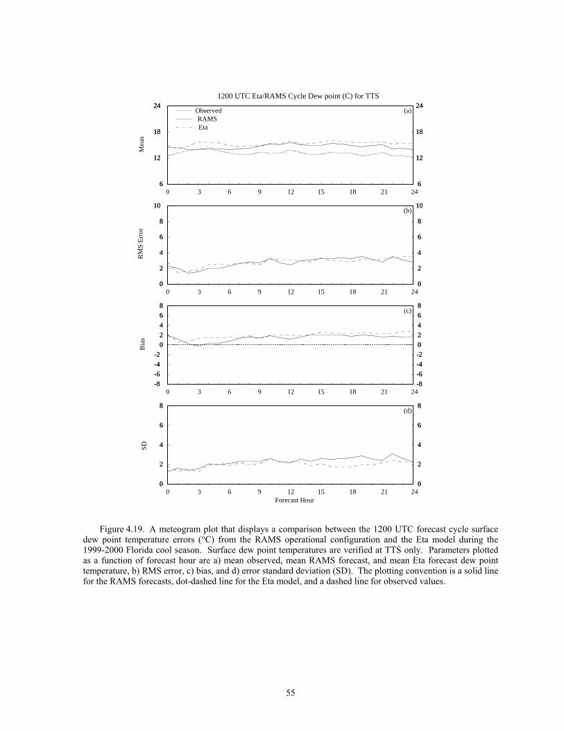
55

6

12

18

24

6

12

18

24

0

2

4

6

8

10

0

2

4

6

8

10

-8

-6

-4

-2

0

2

4

6

8

-8

-6

-4

-2

0

2

4

6

8

10/00 10/02 10/04 10/06 10/08 10/10 10/12 10/14 10/16 10/18 10/20 10/22 11/000

2

4

6

8

0

2

4

6

8

6

12

18

24

6

12

18

24

0

2

4

6

8

10

0

2

4

6

8

10

-8

-6

-4

-2

0

2

4

6

8

-8

-6

-4

-2

0

2

4

6

8

10/00 10/02 10/04 10/06 10/08 10/10 10/12 10/14 10/16 10/18 10/20 10/22 11/000

2

4

6

8

0

2

4

6

8

(a)ObservedRAMS

(b)

(c)

(d)

Mea

nR

MS

Err

orB

ias

SD

0 3 6 9 12 15 18 21 24

0 3 6 9 12 15 18 21 24

0 3 6 9 12 15 18 21 24

0 3 6 9 12 15 18 21 24

Forecast Hour

1200 UTC Eta/RAMS Cycle Dew point (C) for TTS

Eta

Figure 4.19. A meteogram plot that displays a comparison between the 1200 UTC forecast cycle surface

dew point temperature errors (°C) from the RAMS operational configuration and the Eta model during the 1999-2000 Florida cool season. Surface dew point temperatures are verified at TTS only. Parameters plotted as a function of forecast hour are a) mean observed, mean RAMS forecast, and mean Eta forecast dew point temperature, b) RMS error, c) bias, and d) error standard deviation (SD). The plotting convention is a solid line for the RAMS forecasts, dot-dashed line for the Eta model, and a dashed line for observed values.

56

0

20

40

60

80

100

0

20

40

60

80

100

10/00 10/02 10/04 10/06 10/08 10/10 10/12 10/14 10/16 10/18 10/20 10/22 11/00-40

-20

0

20

40

-40

-20

0

20

40

0

20

40

60

80

100

0

20

40

60

80

100

10/00 10/02 10/04 10/06 10/08 10/10 10/12 10/14 10/16 10/18 10/20 10/22 11/00-40

-20

0

20

40

-40

-20

0

20

40

(a)

(b)

RM

S E

rror

Bia

s

0 3 6 9 12 15 18 21 24

0 3 6 9 12 15 18 21 24

Forecast Hour

1200 UTC Eta/RAMS Cycle Wind Dir (deg) for TTS

RAMSEta

Figure 4.20. A meteogram plot that displays a comparison between the 1200 UTC forecast cycle surface

wind direction errors (degrees) from the RAMS operational configuration and the Eta model during the 1999-2000 Florida cool season. Surface wind direction is verified at TTS only. Parameters plotted as a function of forecast hour are a) RMS error and b) bias. The plotting convention is a solid line for the RAMS errors and a dot-dashed line for the Eta model errors.

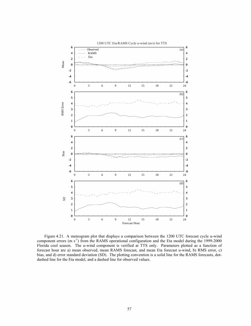
57

-6

-4

-2

0

2

4

6

-6

-4

-2

0

2

4

6

0

1

2

3

4

5

6

0

1

2

3

4

5

6

-6

-4

-2

0

2

4

6

-6

-4

-2

0

2

4

6

10/00 10/02 10/04 10/06 10/08 10/10 10/12 10/14 10/16 10/18 10/20 10/22 11/000

1

2

3

4

5

6

0

1

2

3

4

5

6

-6

-4

-2

0

2

4

6

-6

-4

-2

0

2

4

6

0

1

2

3

4

5

6

0

1

2

3

4

5

6

-6

-4

-2

0

2

4

6

-6

-4

-2

0

2

4

6

10/00 10/02 10/04 10/06 10/08 10/10 10/12 10/14 10/16 10/18 10/20 10/22 11/000

1

2

3

4

5

6

0

1

2

3

4

5

6

(a)ObservedRAMS

(b)

(c)

(d)

Mea

nR

MS

Err

orB

ias

SD

0 3 6 9 12 15 18 21 24

0 3 6 9 12 15 18 21 24

0 3 6 9 12 15 18 21 24

0 3 6 9 12 15 18 21 24

Forecast Hour

Eta

1200 UTC Eta/RAMS Cycle u-wind (m/s) for TTS

Figure 4.21. A meteogram plot that displays a comparison between the 1200 UTC forecast cycle u-wind

component errors (m s-1) from the RAMS operational configuration and the Eta model during the 1999-2000 Florida cool season. The u-wind component is verified at TTS only. Parameters plotted as a function of forecast hour are a) mean observed, mean RAMS forecast, and mean Eta forecast u-wind, b) RMS error, c) bias, and d) error standard deviation (SD). The plotting convention is a solid line for the RAMS forecasts, dot-dashed line for the Eta model, and a dashed line for observed values.

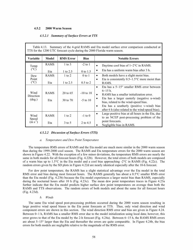
58

4.5.2 2000 Warm Season

4.5.2.1 Summary of Surface Errors at TTS

Table 4.13. Summary of the 4-grid RAMS and Eta model surface error comparison conducted at TTS for the 1200 UTC forecast cycle during the 2000 Florida warm season.

Variable Model RMS Error Bias Notable Errors

Temp (°C)

RAMS

Eta

1 to 3

1 to 2.5

-2 to 1

0 to 1.5

• Daytime cool bias of 1−2°C in RAMS. • Eta has a uniform warm bias after 3 h.

Dew Point (°C)

RAMS

Eta

1 to 2

1 to 2.5

0 to 1

0.5 to 2

• Both models have a slight moist bias. • Eta is consistently 0.5−1.5°C more moist than

RAMS.

Wind Direction

(deg.)

RAMS

Eta

20 to 65

30 to 70

-10 to 18

-5 to 10

• Eta has a 5−15° smaller RMS error between 6−15 h.

• RAMS has a smaller initialization error. • Eta has a larger easterly (negative u-wind)

bias, related to the wind-speed bias. • Eta has a southerly (positive v-wind) bias

after 6 h (also related to the wind-speed bias).

Wind Speed (m s-1)

RAMS

Eta

1 to 2

3 to 5

-1 to 0

2 to 4.5

• Large positive bias at all hours in the Eta, due to an NCEP post-processing problem of the point forecasts.

• Negligible bias in RAMS.

4.5.2.2 Discussion of Surface Errors (TTS)

a. Temperature and Dew Point Temperature

The temperature RMS errors of RAMS and the Eta model are much more similar in the 2000 warm season than during the 1999-2000 cool season. The RAMS and Eta temperature errors for the 2000 warm season are shown in Figure 4.22. With the exception of a few minor deviations, the temperature RMS errors are nearly the same in both models for all forecast hours (Fig. 4.22b). However, the total errors of both models are composed of a warm bias up to 1.5°C in the Eta model and a cool bias approaching -2°C in RAMS (Fig. 4.22c). The random errors given by the SD plots in Figure 4.22d are nearly identical especially after the 10-h forecast.

For dew point temperature, the RAMS has a slight statistical advantage over the Eta model in the total RMS error and bias during most forecast hours. The RAMS generally has about a 0.5°C smaller RMS error than the Eta model (Fig. 4.23b) because the Eta model experiences a larger moist bias than RAMS, especially during the nocturnal hours after 10 h (Fig. 4.23c). The mean dew point temperature traces in Figure 4.23a further indicate that the Eta model predicts higher surface dew point temperatures on average than both the RAMS and TTS observations. The random errors of both models and about the same for all forecast hours (Fig. 4.23d).

b. Winds

The same Eta wind speed post-processing problem occurred during the 2000 warm season resulting in large positive wind speed biases in the Eta point forecasts at TTS. Thus, only wind direction and wind component errors are shown in this section. The wind direction RMS error and bias are given in Figure 4.24. Between 0−1 h, RAMS has a smaller RMS error due to the model initialization using local data; however, this error grows to that of the Eta model by the 2-h forecast (Fig. 4.24a). Between 6−15 h, the RAMS RMS errors are about 5−15° larger than the Eta and thereafter the errors are quite comparable. In Figure 4.24b, the bias errors for both models are negligible relative to the magnitude of the RMS error.

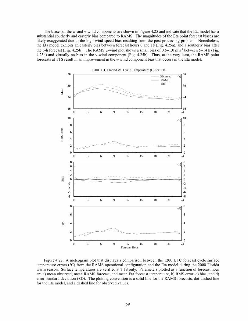
59

The biases of the u- and v-wind components are shown in Figure 4.25 and indicate that the Eta model has a substantial southerly and easterly bias compared to RAMS. The magnitudes of the Eta point forecast biases are likely exaggerated due to the high wind speed bias resulting from the post-processing problem. Nonetheless, the Eta model exhibits an easterly bias between forecast hours 0 and 18 (Fig. 4.25a), and a southerly bias after the 6-h forecast (Fig. 4.25b). The RAMS u-wind plot shows a small bias of 0.5−1.0 m s-1 between 5−14 h (Fig. 4.25a) and virtually no bias in the v-wind component (Fig. 4.25b). Thus, at the very least, the RAMS point forecasts at TTS result in an improvement in the v-wind component bias that occurs in the Eta model.

18

24

30

36

18

24

30

36

0

2

4

6

8

10

0

2

4

6

8

10

-8

-6

-4

-2

0

2

4

6

8

-8

-6

-4

-2

0

2

4

6

8

10/00 10/02 10/04 10/06 10/08 10/10 10/12 10/14 10/16 10/18 10/20 10/22 11/000

2

4

6

8

0

2

4

6

8

18

24

30

36

18

24

30

36

0

2

4

6

8

10

0

2

4

6

8

10

-8

-6

-4

-2

0

2

4

6

8

-8

-6

-4

-2

0

2

4

6

8

10/00 10/02 10/04 10/06 10/08 10/10 10/12 10/14 10/16 10/18 10/20 10/22 11/000

2

4

6

8

0

2

4

6

8

(a)ObservedRAMS

(b)

(c)

(d)

Mea

nR

MS

Err

orB

ias

SD

0 3 6 9 12 15 18 21 24

0 3 6 9 12 15 18 21 24

0 3 6 9 12 15 18 21 24

0 3 6 9 12 15 18 21 24

Forecast Hour

1200 UTC Eta/RAMS Cycle Temperature (C) for TTS

Eta

Figure 4.22. A meteogram plot that displays a comparison between the 1200 UTC forecast cycle surface

temperature errors (°C) from the RAMS operational configuration and the Eta model during the 2000 Florida warm season. Surface temperatures are verified at TTS only. Parameters plotted as a function of forecast hour are a) mean observed, mean RAMS forecast, and mean Eta forecast temperature, b) RMS error, c) bias, and d) error standard deviation (SD). The plotting convention is a solid line for the RAMS forecasts, dot-dashed line for the Eta model, and a dashed line for observed values.

60

12

15

18

21

24

27

12

15

18

21

24

27

0

2

4

6

8

10

0

2

4

6

8

10

-8

-6

-4

-2

0

2

4

6

8

-8

-6

-4

-2

0

2

4

6

8

10/00 10/02 10/04 10/06 10/08 10/10 10/12 10/14 10/16 10/18 10/20 10/22 11/000

2

4

6

8

0

2

4

6

8

12

15

18

21

24

27

12

15

18

21

24

27

0

2

4

6

8

10

0

2

4

6

8

10

-8

-6

-4

-2

0

2

4

6

8

-8

-6

-4

-2

0

2

4

6

8

10/00 10/02 10/04 10/06 10/08 10/10 10/12 10/14 10/16 10/18 10/20 10/22 11/000

2

4

6

8

0

2

4

6

8

(a)

ObservedRAMS

(b)

(c)

(d)

Mea

nR

MS

Err

orB

ias

SD

0 3 6 9 12 15 18 21 24

0 3 6 9 12 15 18 21 24

0 3 6 9 12 15 18 21 24

0 3 6 9 12 15 18 21 24

Forecast Hour

1200 UTC Eta/RAMS Cycle Dew point (C) for TTS

Eta

Figure 4.23. A meteogram plot that displays a comparison between the 1200 UTC forecast cycle surface

dew point temperature errors (°C) from the RAMS operational configuration and the Eta model during the 2000 Florida warm season. Surface dew point temperatures are verified at TTS only. Parameters plotted as a function of forecast hour are a) mean observed, mean RAMS forecast, and mean Eta forecast dew point temperature, b) RMS error, c) bias, and d) error standard deviation (SD). The plotting convention is a solid line for the RAMS forecasts, dot-dashed line for the Eta model, and a dashed line for observed values.

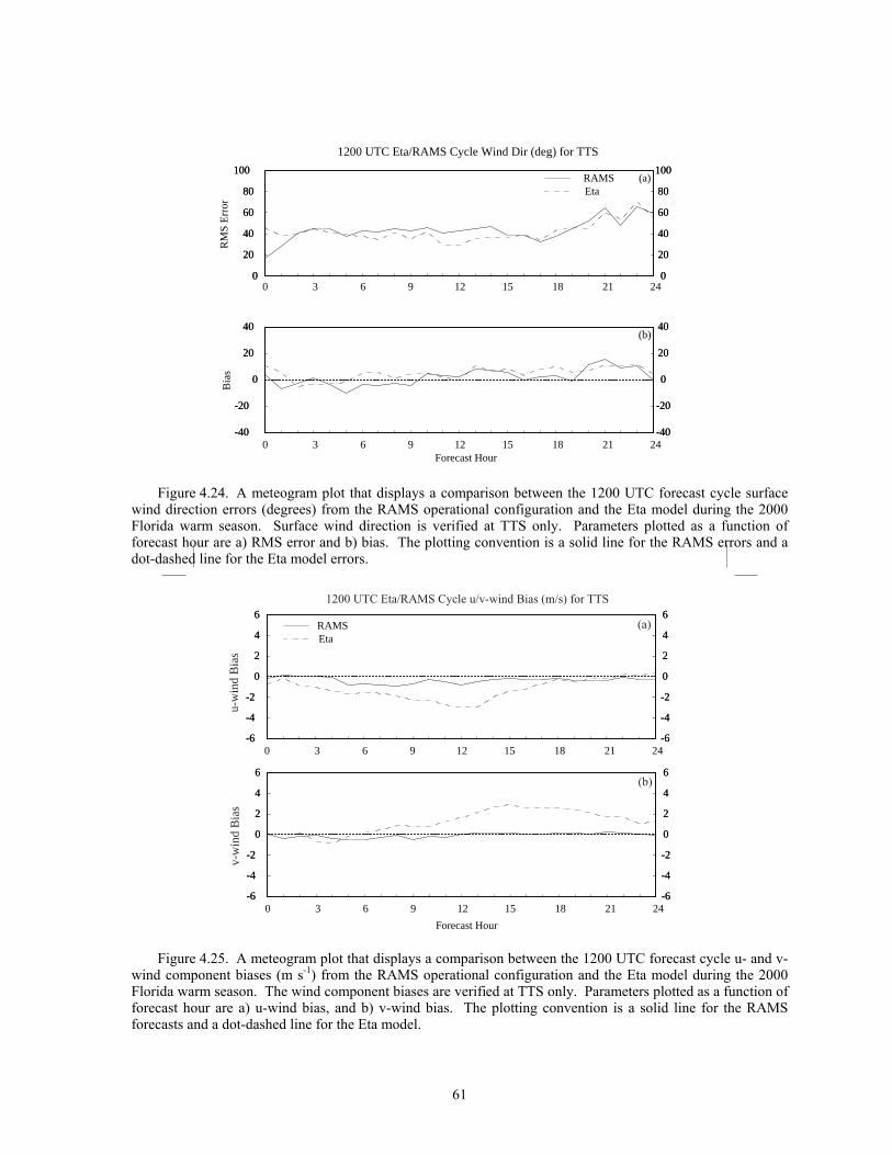
61

0

20

40

60

80

100

0

20

40

60

80

100

10/00 10/02 10/04 10/06 10/08 10/10 10/12 10/14 10/16 10/18 10/20 10/22 11/00-40

-20

0

20

40

-40

-20

0

20

40

0

20

40

60

80

100

0

20

40

60

80

100

10/00 10/02 10/04 10/06 10/08 10/10 10/12 10/14 10/16 10/18 10/20 10/22 11/00-40

-20

0

20

40

-40

-20

0

20

40

(a)

(b)

RM

S E

rror

Bia

s

0 3 6 9 12 15 18 21 24

0 3 6 9 12 15 18 21 24

Forecast Hour

1200 UTC Eta/RAMS Cycle Wind Dir (deg) for TTS

RAMSEta

Figure 4.24. A meteogram plot that displays a comparison between the 1200 UTC forecast cycle surface

wind direction errors (degrees) from the RAMS operational configuration and the Eta model during the 2000 Florida warm season. Surface wind direction is verified at TTS only. Parameters plotted as a function of forecast hour are a) RMS error and b) bias. The plotting convention is a solid line for the RAMS errors and a dot-dashed line for the Eta model errors.

Forecast Hour

-6

-4

-2

0

2

4

6

-6

-4

-2

0

2

4

6

-6

-4

-2

0

2

4

6

-6

-4

-2

0

2

4

6

0 3 6 9 12 15 18 21 24

-6

-4

-2

0

2

4

6

-6

-4

-2

0

2

4

6

-6

-4

-2

0

2

4

6

-6

-4

-2

0

2

4

6

0 3 6 9 12 15 18 21 24

(a)

(b)

u-w

ind

Bia

sv-

win

d B

ias

RAMSEta

1200 UTC Eta/RAMS Cycle u/v-wind Bias (m/s) for TTS

Figure 4.25. A meteogram plot that displays a comparison between the 1200 UTC forecast cycle u- and v-

wind component biases (m s-1) from the RAMS operational configuration and the Eta model during the 2000 Florida warm season. The wind component biases are verified at TTS only. Parameters plotted as a function of forecast hour are a) u-wind bias, and b) v-wind bias. The plotting convention is a solid line for the RAMS forecasts and a dot-dashed line for the Eta model.

62

4.5.3 Summary of RAMS/Eta Error Comparison

Based on the surface objective error statistics at TTS during the 1999-2000 cool, and 1999 and 2000 warm seasons, the following conclusions can be made:

• RAMS has a 1−2°C larger temperature error during the cool season due to the prevailing surface cold bias.

• The two models have comparable total errors during the warm season, composed of separate types of biases. The Eta has a 1−1.5°C warm bias while RAMS has a 1−2°C cold bias.

• Eta has a cool-season nocturnal warm bias whereas RAMS has no nocturnal bias.

• Both models have a moist bias during the cool season (0.5−1.0°C smaller in RAMS) but only the Eta has a moist bias in the warm season. Thus, RAMS total dew point temperature errors are slightly improved over the Eta during the warm season.

• The Eta model has 5−15° smaller wind direction errors during both seasons. During the warm season, the Eta wind direction errors are smaller mainly during the afternoon and evening hours.

• In the cool season, RAMS has more of a nocturnal easterly wind bias than the Eta model.

• In the warm season, the Eta model has a greater southerly and easterly wind bias than the RAMS.

• Overall, the RAMS model does not exhibit dramatically improved error statistics over the Eta model.

The subjective sea-breeze comparison between RAMS and the Eta model at TTS is presented in Section 5.2.1.3. These results will show that the objective error statistics are not sufficient in illustrating the potential added value of a local, high-resolution model such as RAMS. The combination of objective and subjective evaluation is necessary to adequately verify fine-scale forecasts such as those generated by RAMS in east-central Florida.

4.6 Gridded Error Statistics

The final portion of the RAMS objective verification is a comparison between objectively-analyzed KSC/CCAFS wind-tower observations and forecast gridded data over the area of grid 4. Objective error statistics such as RMS error and bias were computed at all available grid points on RAMS grid 4 where observational data influenced the objective analysis. Based on the spatial and temporal distribution of error statistics for temperature and winds, no significant additional information was obtained in this experiment. The results of the gridded error statistics were consistent with the point forecast error statistics for the KSC/CCAFS wind towers, and little additional information added to our understanding of the nature of RAMS errors within the area of the KSC/CCAFS wind towers.

The factor that most limited the value added from this exercise is the fact that very few (if any) observations are available over the rivers and immediate oceanic regions. As a result, the error statistics experienced unrepresentative gradients along the coastlines and river boundaries, caused by larger errors over water since RAMS is able to resolve the temperature and wind differences between water and land areas. Since nearly all of the wind towers are located over land only, the objective analysis of tower observations is valid only for land areas and does not include any information about temperature, wind, and moisture over the Banana and Indian rivers. Essentially, the KSC/CCAFS observational network is not sufficient to verify the spatial gradients of the RAMS forecasts from the 1.25-km resolution grid. This situation illustrates one of the major difficulties in verifying NWP models run at very high spatial resolutions. To verify adequately this type of configured NWP model, the observational network must have sufficiently high spatial and temporal resolution to resolve the features predicted.

63

5. Subjective Evaluation Results

This section presents results from an extensive number of subjective verification experiments for both the 1999-2000 cool, and 1999 and 2000 warm seasons. The 1999-2000 cool-season subjective verification results include:

• Frontal passages at seven east coast stations in Section 5.1.1.

• Cool-season precipitation verification in Section 5.1.2. During the 1999-2000 cool season, very few significant precipitation events occurred and thus, Section 5.1.2 includes only a brief summary of the events that occurred along with two precipitation examples.

• Low-level temperature inversions at the XMR rawinsonde in Section 5.1.3.

The warm season results also include three components:

• Sea-breeze verification at the KSC/CCAFS wind towers and at TTS for 1999 and 2000 forecasts presented in Section 5.2.1.

• Precipitation validation on RAMS grid 4 for the 2000 months shown in Section 5.2.2.

• Thunderstorm initiation verification for the 2000 months given in Section 5.2.3.

Even though the ERDAS RAMS interim report contained the 1999 warm season sea-breeze verification results, the AMU evaluated these sea-breeze forecasts again for two reasons. First, the AMU modified the evaluation technique to include all available archived forecast data for both the 1999 and 2000 warm seasons compared to data only during AMU working days, as was done in the interim report on the 1999 data. Second, by performing the evaluation for all available archived forecasts, the AMU could build a database of sea-breeze verification statistics for two Florida warm seasons, thereby increasing the robustness of the results. It is important to note that the 1999 database contains forecasts during the months of May−August whereas the 2000 warm season database contains forecasts for May−September.

The precipitation and thunderstorm initiation verifications are performed on the 2000 warm season forecasts only, as tasked in the ERDAS RAMS extension evaluation. The precipitation verification closely follows the technique used in the ERDAS RAMS interim report, but with a few modifications (refer to Section 2.2.2.2 and Case 2000). As with the sea-breeze evaluation, the precipitation verification was modified from the technique used for the 1999 warm season to include all available archived forecasts during the 2000 warm season in order to maximize the verification data base. However, the appropriate WSR-74C reflectivity fields for the precipitation verification were not archived until late May 2000. Thus, the precipitation verification is performed only for the months of June−September 2000. The thunderstorm initiation verification was conducted for all 2000 warm season months (May−September).

5.1 1999-2000 Cool Season

The results from the 1999-2000 Florida cool-season subjective verification are presented in this section. All three components of the cool-season subjective verification were conducted from November 1999 to March 2000. Refer to Section 2.2.1 for the methodology used in each experiment.

5.1.1 Verification of Fronts

During the five cool-season months, the AMU documented all occurrences of any type of observed frontal discontinuities (wind shifts, temperature, or dew point temperature gradients). Graphical traces (meteograms) of observed and forecast hourly temperature, dew point temperature, wind direction, wind speed, and pressure observations were examined at seven selected surface stations in the Florida peninsula [Jacksonville (JAX), Daytona Beach (DAB), the Shuttle Landing Facility (TTS), Melbourne (MLB), Vero Beach (VRB), West Palm Beach (PBI), and Miami (MIA)]. Figure 5.1 shows a sample meteogram from 22 December 1999 illustrating the evolution of forecast and observed variables during the passage of a weak front at TTS. Note the smooth transition in the forecast wind shift compared to the observed wind shift in Figure 5.1b. From 1400−1500 UTC, the observed wind direction changes sharply from southwesterly (~240°) to northwesterly (> 300°). Meanwhile, the RAMS forecast has a very gradual shift from south-southwesterly winds at 1400 UTC to

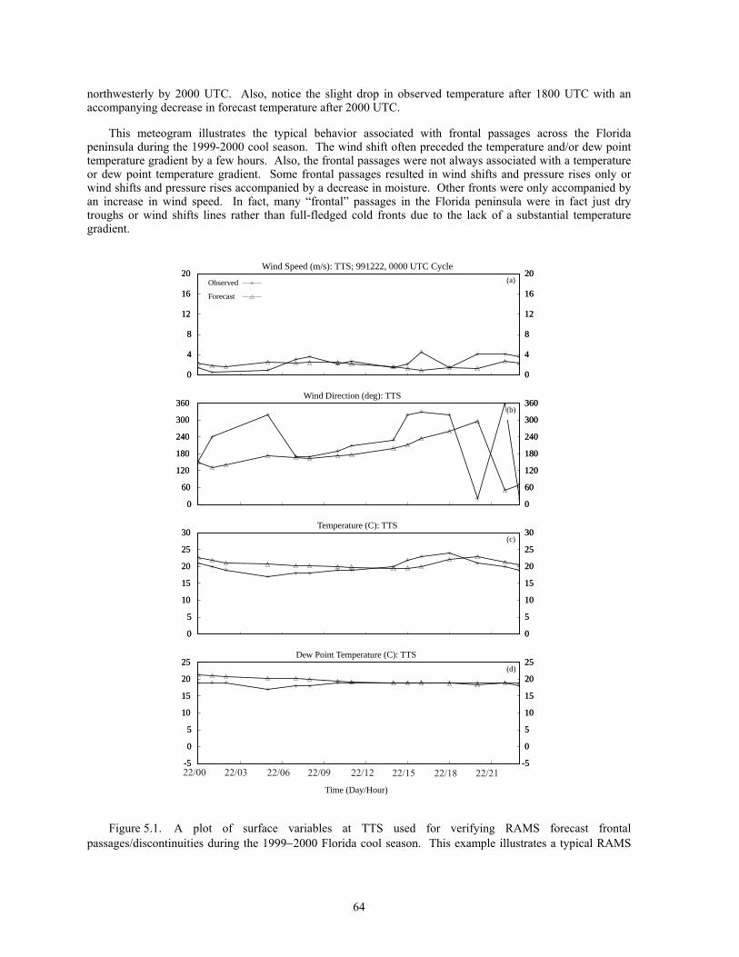
64

northwesterly by 2000 UTC. Also, notice the slight drop in observed temperature after 1800 UTC with an accompanying decrease in forecast temperature after 2000 UTC.

This meteogram illustrates the typical behavior associated with frontal passages across the Florida peninsula during the 1999-2000 cool season. The wind shift often preceded the temperature and/or dew point temperature gradient by a few hours. Also, the frontal passages were not always associated with a temperature or dew point temperature gradient. Some frontal passages resulted in wind shifts and pressure rises only or wind shifts and pressure rises accompanied by a decrease in moisture. Other fronts were only accompanied by an increase in wind speed. In fact, many “frontal” passages in the Florida peninsula were in fact just dry troughs or wind shifts lines rather than full-fledged cold fronts due to the lack of a substantial temperature gradient.

0

4

8

12

16

20

0

4

8

12

16

20

0

60

120

180

240

300

360

0

60

120

180

240

300

360

0

5

10

15

20

25

30

0

5

10

15

20

25

30

-5

0

5

10

15

20

25

-5

0

5

10

15

20

25

0

4

8

12

16

20

0

4

8

12

16

20

0

60

120

180

240

300

360

0

60

120

180

240

300

360

0

5

10

15

20

25

30

0

5

10

15

20

25

30

-5

0

5

10

15

20

25

-5

0

5

10

15

20

25Dew Point Temperature (C): TTS

Temperature (C): TTS

Wind Direction (deg): TTS

Wind Speed (m/s): TTS; 991222, 0000 UTC Cycle

Observed

Forecast

Time (Day/Hour)

(a)

(b)

(c)

(d)

22/00 22/03 22/06 22/09 22/12 22/15 22/18 22/21

Figure 5.1. A plot of surface variables at TTS used for verifying RAMS forecast frontal

passages/discontinuities during the 1999−2000 Florida cool season. This example illustrates a typical RAMS

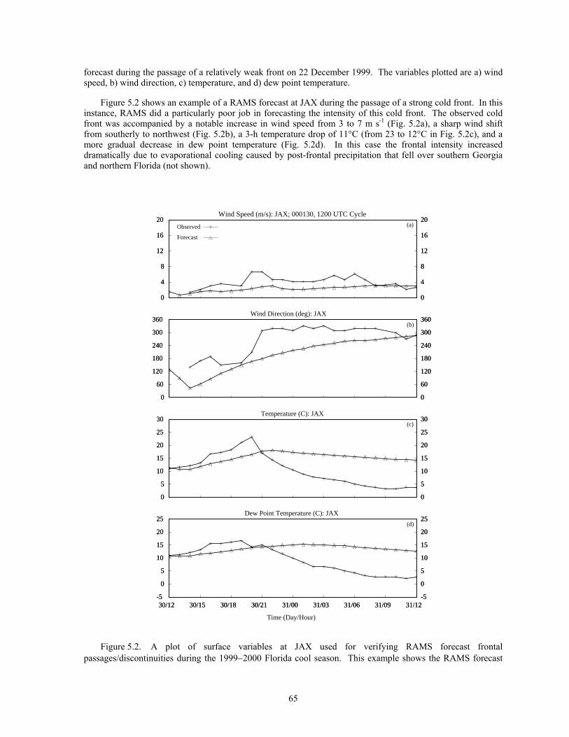
65

forecast during the passage of a relatively weak front on 22 December 1999. The variables plotted are a) wind speed, b) wind direction, c) temperature, and d) dew point temperature.

Figure 5.2 shows an example of a RAMS forecast at JAX during the passage of a strong cold front. In this instance, RAMS did a particularly poor job in forecasting the intensity of this cold front. The observed cold front was accompanied by a notable increase in wind speed from 3 to 7 m s-1 (Fig. 5.2a), a sharp wind shift from southerly to northwest (Fig. 5.2b), a 3-h temperature drop of 11°C (from 23 to 12°C in Fig. 5.2c), and a more gradual decrease in dew point temperature (Fig. 5.2d). In this case the frontal intensity increased dramatically due to evaporational cooling caused by post-frontal precipitation that fell over southern Georgia and northern Florida (not shown).

0

4

8

12

16

20

0

4

8

12

16

20

0

60

120

180

240

300

360

0

60

120

180

240

300

360

0

5

10

15

20

25

30

0

5

10

15

20

25

30

30/12 30/15 30/18 30/21 31/00 31/03 31/06 31/09 31/12-5

0

5

10

15

20

25

-5

0

5

10

15

20

25

0

4

8

12

16

20

0

4

8

12

16

20

0

60

120

180

240

300

360

0

60

120

180

240

300

360

0

5

10

15

20

25

30

0

5

10

15

20

25

30

30/12 30/15 30/18 30/21 31/00 31/03 31/06 31/09 31/12-5

0

5

10

15

20

25

-5

0

5

10

15

20

25Dew Point Temperature (C): JAX

Temperature (C): JAX

Wind Direction (deg): JAX

Wind Speed (m/s): JAX; 000130, 1200 UTC Cycle

Observed

Forecast

Time (Day/Hour)

(a)

(b)

(c)

(d)

Figure 5.2. A plot of surface variables at JAX used for verifying RAMS forecast frontal

passages/discontinuities during the 1999−2000 Florida cool season. This example shows the RAMS forecast

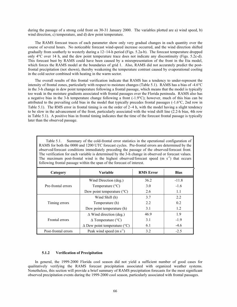
66

during the passage of a strong cold front on 30-31 January 2000. The variables plotted are a) wind speed, b) wind direction, c) temperature, and d) dew point temperature.

The RAMS forecast traces of each parameter show only very gradual changes in each quantity over the course of several hours. No noticeable forecast wind-speed increase occurred, and the wind direction shifted gradually from southerly to westerly during a 12−14-h period (Figs. 5.2a-b). The forecast temperature dropped only 4°C over 14 h, and the dew point temperature trace does not indicate any discontinuity (Figs. 5.2c-d). This forecast bust by RAMS could have been caused by a misrepresentation of the front in the Eta model, which forces the RAMS model at the boundaries of grid 1. Also, RAMS did not accurately predict the post-frontal precipitation (not shown), thereby weakening the temperature contrast caused by evaporational cooling in the cold sector combined with heating in the warm sector.

The overall results of this frontal verification indicate that RAMS has a tendency to under-represent the intensity of frontal zones, particularly with respect to moisture changes (Table 5.1). RAMS has a bias of -4.6°C in the 3-h change in dew point temperature following a frontal passage, which means that the model is typically too weak in the moisture gradients associated with frontal passages over the Florida peninsula. RAMS also has a negative bias in the 3-h temperature change following a front (-1.9°C); however, much of this bias can be attributed to the prevailing cold bias in the model that typically precedes frontal passages (-1.6°C, 2nd row in Table 5.1). The RMS error in frontal timing is on the order of 2−4 h, with the model having a slight tendency to be slow in the advancement of the front, particularly associated with the wind shift line (2.2-h bias, 4th row in Table 5.1). A positive bias in frontal timing indicates that the time of the forecast frontal passage is typically later than the observed passage.

Table 5.1. Summary of the cold-frontal error statistics in the operational configuration of RAMS for both the 0000 and 1200 UTC forecast cycles. Pre-frontal errors are determined by the observed/forecast conditions immediately preceding the passage of the observed/forecast front. The verification for each variable is determined by the 3-h change in observed or forecast values. The maximum post-frontal wind is the highest observed/forecast speed (m s-1) that occurs following frontal passage within the span of the forecast of interest.

Category Variable RMS Error Bias

Wind Direction (deg.) 36.2 -11.8 Pre-frontal errors Temperature (°C) 3.0 -1.6

Dew point temperature (°C) 2.6 1.1 Wind Shift (h) 3.7 2.2

Timing errors Temperature (h) 2.2 0.2 Dew point temperature (h) 3.1 1.2 ∆ Wind direction (deg.) 46.9 1.9

Frontal errors ∆ Temperature (°C) 3.1 -1.9 ∆ Dew point temperature (°C) 6.1 -4.6

Post-frontal errors Peak wind speed (m s-1) 3.2 -2.5

5.1.2 Verification of Precipitation

In general, the 1999-2000 Florida cool season did not yield a sufficient number of good cases for qualitatively verifying the RAMS forecast precipitation associated with organized weather systems. Nonetheless, this section will provide a brief summary of RAMS precipitation forecasts for the most significant observed precipitation events during the 1999-2000 cool season, particularly associated with frontal passages.

67

Table 5.2 summarizes the seven most substantial precipitation events during the 1999-2000 cool season. Based on these events, RAMS performed with variable accuracy when forecasting cool-season precipitation events across the Florida peninsula. RAMS generally did not accurately predict the timing and location of pre-frontal rain bands, but could handle the rain bands associated with the actual cold front better. With some events such as 17 December 1999 and 31 January 2000, RAMS did not predict any substantial precipitation despite the occurrence of fairly widespread observed rainfall. In the 2 November 1999 cold front and associated squall line, the timing of the frontal passage was substantially in error and thus, the rainfall was not predicted well at all. In the 12 March and 27 March 2000 frontal events, RAMS did not predict the significant convection that occurred over southern Florida, but accurately predicted the lighter precipitation over central Florida.

Figure 5.3 shows an example of how RAMS missed the pre-frontal rain band during the 24 January 2000 strong frontal passage over the Florida peninsula. This figure also illustrates the accurate prediction of the frontal band; however, most of the precipitation fell with the pre-frontal squall line, so the forecast rainfall rates are much too high associated with the frontal passage. At 0900 UTC, a substantial amount of convection is prevalent across the Florida peninsula, especially concentrated over the southern and eastern portions (Fig. 5.3a). RAMS does not indicate forecast precipitation in any portion of the grid-2 domain at this time. The squall line has cleared much of the peninsula by 1200 UTC when a second band of convection becomes prevalent across the northwestern portions of grid 2 (Fig. 5.3b). Between 1500−1800 UTC, the frontal band quickly moves into central Florida and weakens noticeably by 1800 UTC (Figs. 5.3c-d). At these times, RAMS predicts a fairly intense rain band associated with the second observed cloud band with rainfall rates exceeding 40 mm h-1 in some instances. However, only light precipitation occurred with the passage of the frontal band since most of the heaviest rainfall occurred with the pre-frontal rain band. This case shows how RAMS had difficulty in predicting pre-frontal squall lines during the 1999-2000 cool-season precipitation events.

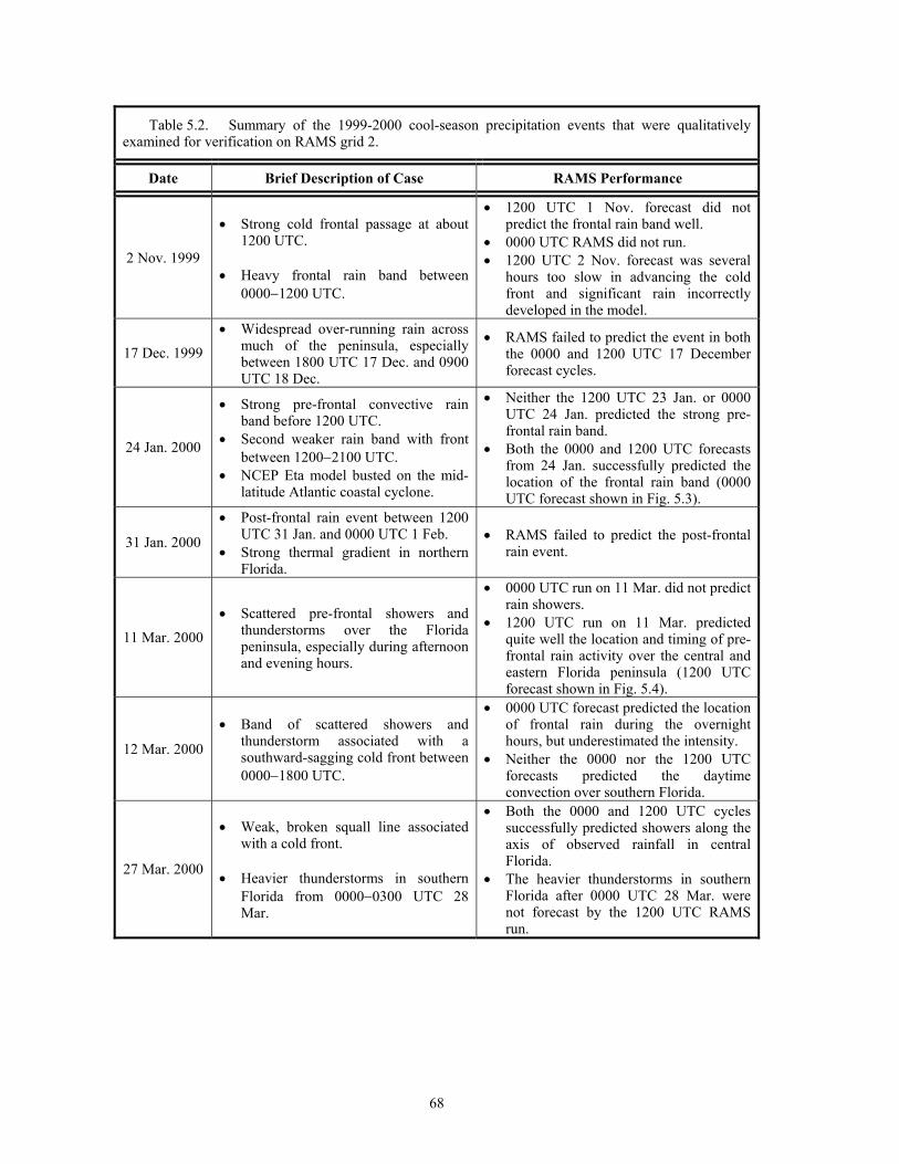
68

Table 5.2. Summary of the 1999-2000 cool-season precipitation events that were qualitatively examined for verification on RAMS grid 2.

Date Brief Description of Case RAMS Performance

2 Nov. 1999

• Strong cold frontal passage at about 1200 UTC.

• Heavy frontal rain band between

0000−1200 UTC.

• 1200 UTC 1 Nov. forecast did not predict the frontal rain band well.

• 0000 UTC RAMS did not run. • 1200 UTC 2 Nov. forecast was several

hours too slow in advancing the cold front and significant rain incorrectly developed in the model.

17 Dec. 1999 • Widespread over-running rain across

much of the peninsula, especially between 1800 UTC 17 Dec. and 0900 UTC 18 Dec.

• RAMS failed to predict the event in both the 0000 and 1200 UTC 17 December forecast cycles.

24 Jan. 2000

• Strong pre-frontal convective rain band before 1200 UTC.

• Second weaker rain band with front between 1200−2100 UTC.

• NCEP Eta model busted on the mid-latitude Atlantic coastal cyclone.

• Neither the 1200 UTC 23 Jan. or 0000 UTC 24 Jan. predicted the strong pre-frontal rain band.

• Both the 0000 and 1200 UTC forecasts from 24 Jan. successfully predicted the location of the frontal rain band (0000 UTC forecast shown in Fig. 5.3).

31 Jan. 2000

• Post-frontal rain event between 1200 UTC 31 Jan. and 0000 UTC 1 Feb.

• Strong thermal gradient in northern Florida.

• RAMS failed to predict the post-frontal rain event.

11 Mar. 2000 • Scattered pre-frontal showers and

thunderstorms over the Florida peninsula, especially during afternoon and evening hours.

• 0000 UTC run on 11 Mar. did not predict rain showers.

• 1200 UTC run on 11 Mar. predicted quite well the location and timing of pre-frontal rain activity over the central and eastern Florida peninsula (1200 UTC forecast shown in Fig. 5.4).

12 Mar. 2000

• Band of scattered showers and thunderstorm associated with a southward-sagging cold front between 0000−1800 UTC.

• 0000 UTC forecast predicted the location of frontal rain during the overnight hours, but underestimated the intensity.

• Neither the 0000 nor the 1200 UTC forecasts predicted the daytime convection over southern Florida.

27 Mar. 2000

• Weak, broken squall line associated with a cold front.

• Heavier thunderstorms in southern

Florida from 0000−0300 UTC 28 Mar.

• Both the 0000 and 1200 UTC cycles successfully predicted showers along the axis of observed rainfall in central Florida.

• The heavier thunderstorms in southern Florida after 0000 UTC 28 Mar. were not forecast by the 1200 UTC RAMS run.

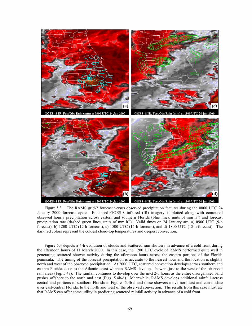
69

Figure 5.3. The RAMS grid-2 forecast versus observed precipitation features during the 0000 UTC 24

January 2000 forecast cycle. Enhanced GOES-8 infrared (IR) imagery is plotted along with contoured observed hourly precipitation across eastern and southern Florida (blue lines, units of mm h-1) and forecast precipitation rate (dashed green lines, units of mm h-1). Valid times on 24 January are: a) 0900 UTC (9-h forecast), b) 1200 UTC (12-h forecast), c) 1500 UTC (15-h forecast), and d) 1800 UTC (18-h forecast). The dark red colors represent the coldest cloud-top temperatures and deepest convection.

Figure 5.4 depicts a 4-h evolution of clouds and scattered rain showers in advance of a cold front during the afternoon hours of 11 March 2000. In this case, the 1200 UTC cycle of RAMS performed quite well in generating scattered shower activity during the afternoon hours across the eastern portions of the Florida peninsula. The timing of the forecast precipitation is accurate to the nearest hour and the location is slightly north and west of the observed precipitation. At 2000 UTC, scattered convection develops across southern and eastern Florida close to the Atlantic coast whereas RAMS develops showers just to the west of the observed rain areas (Fig. 5.4a). The rainfall continues to develop over the next 2-3 hours as the entire disorganized band pushes offshore to the north and east (Figs. 5.4b-d). Meanwhile, RAMS develops additional rainfall across central and portions of southern Florida in Figures 5.4b-d and these showers move northeast and consolidate over east-central Florida, to the north and west of the observed convection. The results from this case illustrate that RAMS can offer some utility in predicting scattered rainfall activity in advance of a cold front.

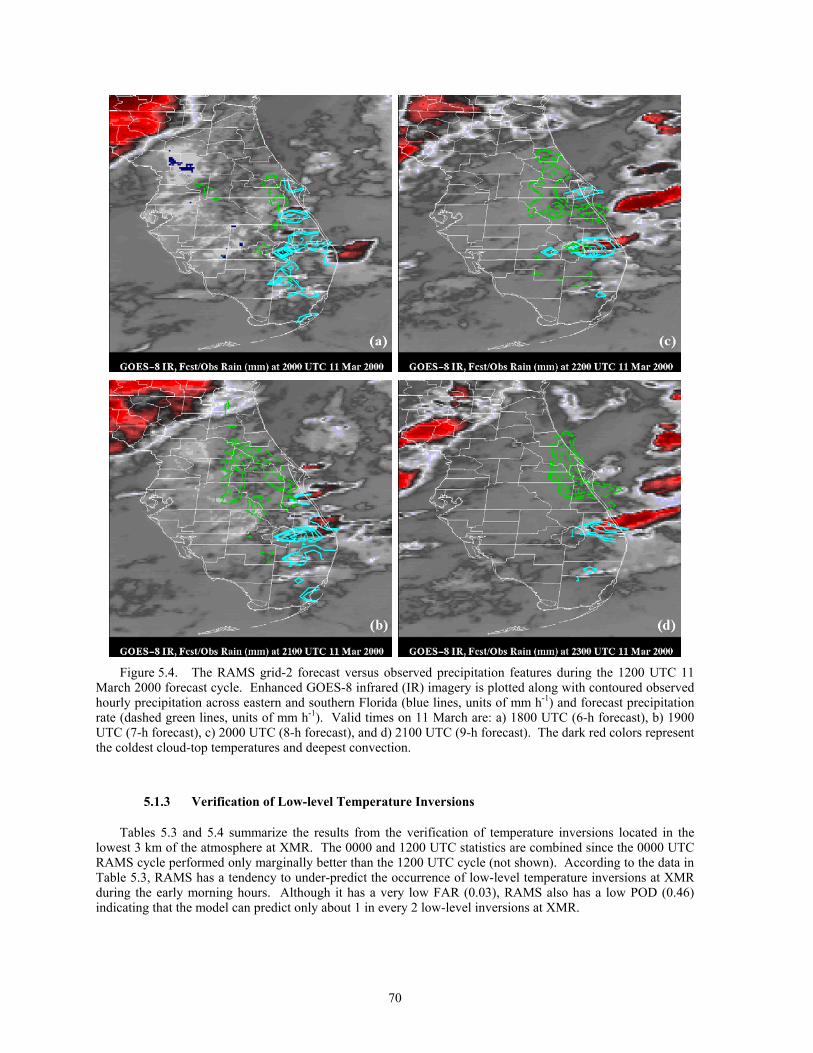
70

Figure 5.4. The RAMS grid-2 forecast versus observed precipitation features during the 1200 UTC 11

March 2000 forecast cycle. Enhanced GOES-8 infrared (IR) imagery is plotted along with contoured observed hourly precipitation across eastern and southern Florida (blue lines, units of mm h-1) and forecast precipitation rate (dashed green lines, units of mm h-1). Valid times on 11 March are: a) 1800 UTC (6-h forecast), b) 1900 UTC (7-h forecast), c) 2000 UTC (8-h forecast), and d) 2100 UTC (9-h forecast). The dark red colors represent the coldest cloud-top temperatures and deepest convection.

5.1.3 Verification of Low-level Temperature Inversions

Tables 5.3 and 5.4 summarize the results from the verification of temperature inversions located in the lowest 3 km of the atmosphere at XMR. The 0000 and 1200 UTC statistics are combined since the 0000 UTC RAMS cycle performed only marginally better than the 1200 UTC cycle (not shown). According to the data in Table 5.3, RAMS has a tendency to under-predict the occurrence of low-level temperature inversions at XMR during the early morning hours. Although it has a very low FAR (0.03), RAMS also has a low POD (0.46) indicating that the model can predict only about 1 in every 2 low-level inversions at XMR.

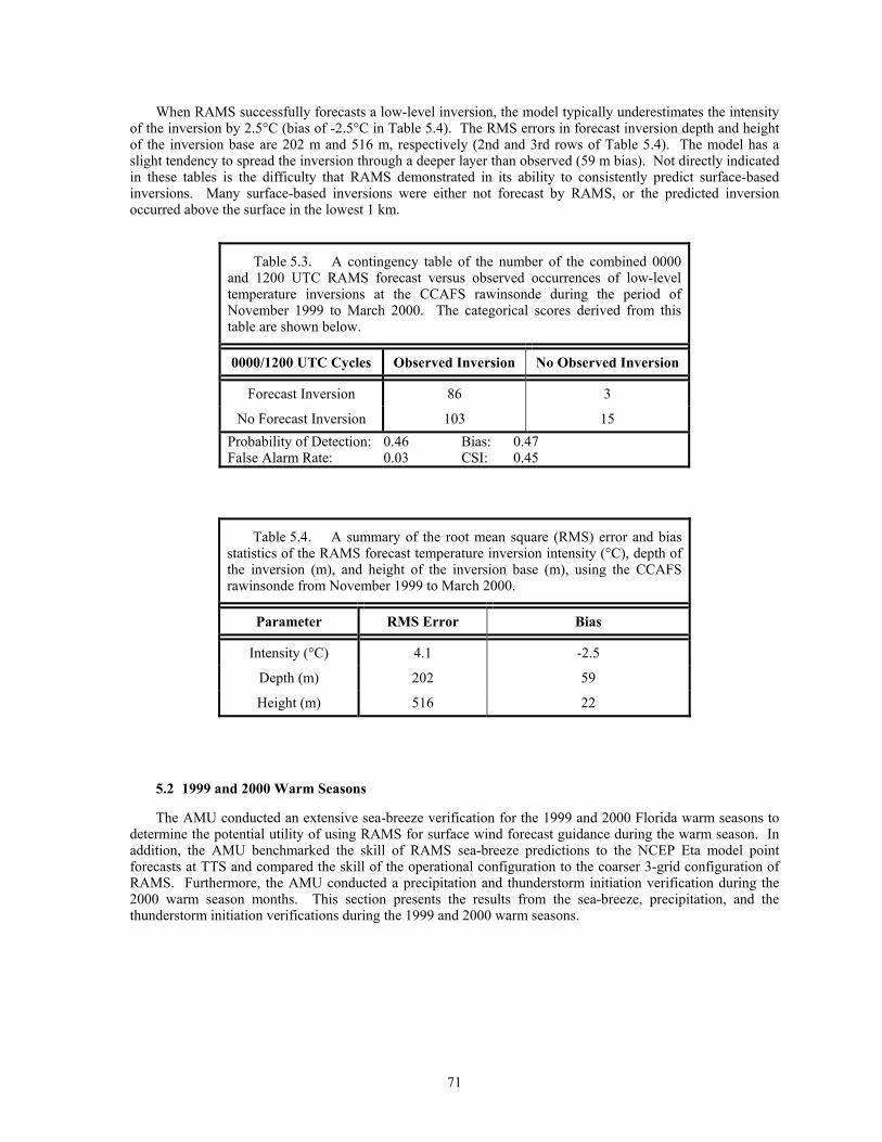
71

When RAMS successfully forecasts a low-level inversion, the model typically underestimates the intensity of the inversion by 2.5°C (bias of -2.5°C in Table 5.4). The RMS errors in forecast inversion depth and height of the inversion base are 202 m and 516 m, respectively (2nd and 3rd rows of Table 5.4). The model has a slight tendency to spread the inversion through a deeper layer than observed (59 m bias). Not directly indicated in these tables is the difficulty that RAMS demonstrated in its ability to consistently predict surface-based inversions. Many surface-based inversions were either not forecast by RAMS, or the predicted inversion occurred above the surface in the lowest 1 km.

Table 5.3. A contingency table of the number of the combined 0000 and 1200 UTC RAMS forecast versus observed occurrences of low-level temperature inversions at the CCAFS rawinsonde during the period of November 1999 to March 2000. The categorical scores derived from this table are shown below.

0000/1200 UTC Cycles Observed Inversion No Observed Inversion

Forecast Inversion 86 3

No Forecast Inversion 103 15 Probability of Detection: 0.46 Bias: 0.47 False Alarm Rate: 0.03 CSI: 0.45

Table 5.4. A summary of the root mean square (RMS) error and bias statistics of the RAMS forecast temperature inversion intensity (°C), depth of the inversion (m), and height of the inversion base (m), using the CCAFS rawinsonde from November 1999 to March 2000.

Parameter RMS Error Bias

Intensity (°C) 4.1 -2.5

Depth (m) 202 59

Height (m) 516 22

5.2 1999 and 2000 Warm Seasons

The AMU conducted an extensive sea-breeze verification for the 1999 and 2000 Florida warm seasons to determine the potential utility of using RAMS for surface wind forecast guidance during the warm season. In addition, the AMU benchmarked the skill of RAMS sea-breeze predictions to the NCEP Eta model point forecasts at TTS and compared the skill of the operational configuration to the coarser 3-grid configuration of RAMS. Furthermore, the AMU conducted a precipitation and thunderstorm initiation verification during the 2000 warm season months. This section presents the results from the sea-breeze, precipitation, and the thunderstorm initiation verifications during the 1999 and 2000 warm seasons.

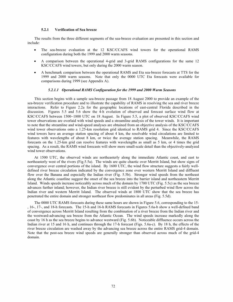
72

5.2.1 Verification of Sea breeze

The results from the three different segments of the sea-breeze evaluation are presented in this section and include:

• The sea-breeze evaluation at the 12 KSC/CCAFS wind towers for the operational RAMS configuration during both the 1999 and 2000 warm seasons.

• A comparison between the operational 4-grid and 3-grid RAMS configurations for the same 12 KSC/CCAFS wind towers, but only during the 2000 warm season.

• A benchmark comparison between the operational RAMS and Eta sea-breeze forecasts at TTS for the 1999 and 2000 warm seasons. Note that only the 0000 UTC Eta forecasts were available for comparisons during 1999 (see Appendix A).

5.2.1.1 Operational RAMS Configuration for the 1999 and 2000 Warm Seasons

This section begins with a sample sea-breeze passage from 18 August 2000 to provide an example of the sea-breeze verification procedure and to illustrate the capability of RAMS in resolving the sea and river breeze interactions. Refer to Figure 2.2a for the geographic locations of east-central Florida described in the discussion. Figures 5.5 and 5.6 show the 4-h evolution of observed and forecast surface wind flow at KSC/CCAFS between 1500−1800 UTC on 18 August. In Figure 5.5, a plot of observed KSC/CCAFS wind tower observations are overlaid with wind speeds and a streamline analysis of the tower winds. It is important to note that the streamline and wind-speed analyses are obtained from an objective analysis of the KSC/CCAFS wind tower observations onto a 1.25-km resolution grid identical to RAMS grid 4. Since the KSC/CCAFS wind towers have an average station spacing of about 4 km, the resolvable wind circulations are limited to features with wavelengths of about 8 km, or twice the average station spacing. Meanwhile, the RAMS forecasts on the 1.25-km grid can resolve features with wavelengths as small as 5 km, or 4 times the grid spacing. As a result, the RAMS wind forecasts will show more small-scale detail than the objectively-analyzed wind tower observations.

At 1500 UTC, the observed winds are northeasterly along the immediate Atlantic coast, and east to northeasterly west of the rivers (Fig.5.5a). The winds are quite chaotic over Merritt Island, but show signs of convergence over central portions of the island. By 1600 UTC, the wind flow structure suggests a fairly well-defined river breeze circulation indicated by the convergence zone over western Merritt Island and diffluent flow over the Banana and especially the Indian river (Fig. 5.5b). Stronger wind speeds from the northeast along the Atlantic coastline suggest the onset of the sea breeze into the barrier island and northeastern Merritt Island. Winds speeds increase noticeably across much of the domain by 1700 UTC (Fig. 5.5c) as the sea breeze advances further inland; however, the Indian river breeze is still evident by the perturbed wind flow across the Indian river and western Merritt Island. The observed winds at 1800 UTC show that the sea breeze has penetrated the entire domain and stronger northeast flow predominates in all areas (Fig. 5.5d).

The 0000 UTC RAMS forecasts during these same hours are shown in Figure 5.6, corresponding to the 15-, 16-, 17-, and 18-h forecasts. The 15-h and 16-h RAMS forecasts in Figures 5.6a-b show a well-defined band of convergence across Merritt Island resulting from the combination of a river breeze from the Indian river and the westward-advancing sea breeze from the Atlantic Ocean. The wind speeds increase markedly along the coast by 16 h as the sea breeze begins to advance westward (Fig. 5.6b). Noticeable diffluence occurs across the Indian river at 15 and 16 h, and continues through the 17-h forecast (Figs. 5.6a-c). By 18 h, the effects of the river breeze circulation are washed away by the advancing sea breeze across the entire RAMS grid-4 domain. Note that the post-sea breeze wind speeds are generally stronger than observed across much of the grid-4 domain.

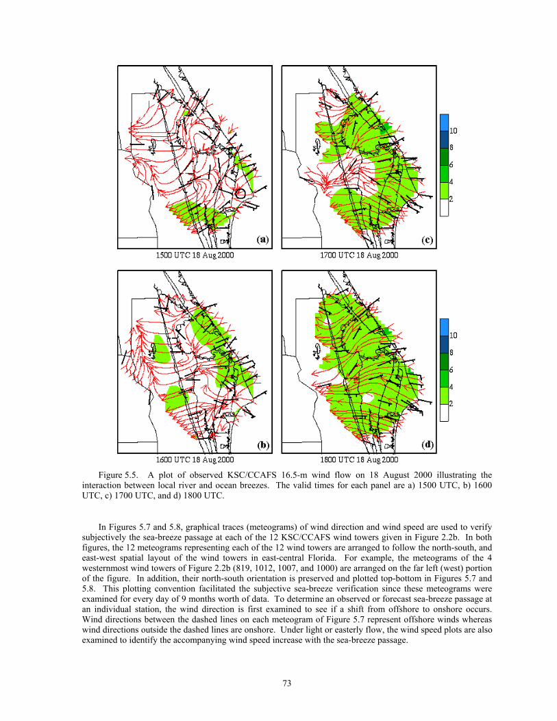
73

Figure 5.5. A plot of observed KSC/CCAFS 16.5-m wind flow on 18 August 2000 illustrating the

interaction between local river and ocean breezes. The valid times for each panel are a) 1500 UTC, b) 1600 UTC, c) 1700 UTC, and d) 1800 UTC.

In Figures 5.7 and 5.8, graphical traces (meteograms) of wind direction and wind speed are used to verify subjectively the sea-breeze passage at each of the 12 KSC/CCAFS wind towers given in Figure 2.2b. In both figures, the 12 meteograms representing each of the 12 wind towers are arranged to follow the north-south, and east-west spatial layout of the wind towers in east-central Florida. For example, the meteograms of the 4 westernmost wind towers of Figure 2.2b (819, 1012, 1007, and 1000) are arranged on the far left (west) portion of the figure. In addition, their north-south orientation is preserved and plotted top-bottom in Figures 5.7 and 5.8. This plotting convention facilitated the subjective sea-breeze verification since these meteograms were examined for every day of 9 months worth of data. To determine an observed or forecast sea-breeze passage at an individual station, the wind direction is first examined to see if a shift from offshore to onshore occurs. Wind directions between the dashed lines on each meteogram of Figure 5.7 represent offshore winds whereas wind directions outside the dashed lines are onshore. Under light or easterly flow, the wind speed plots are also examined to identify the accompanying wind speed increase with the sea-breeze passage.

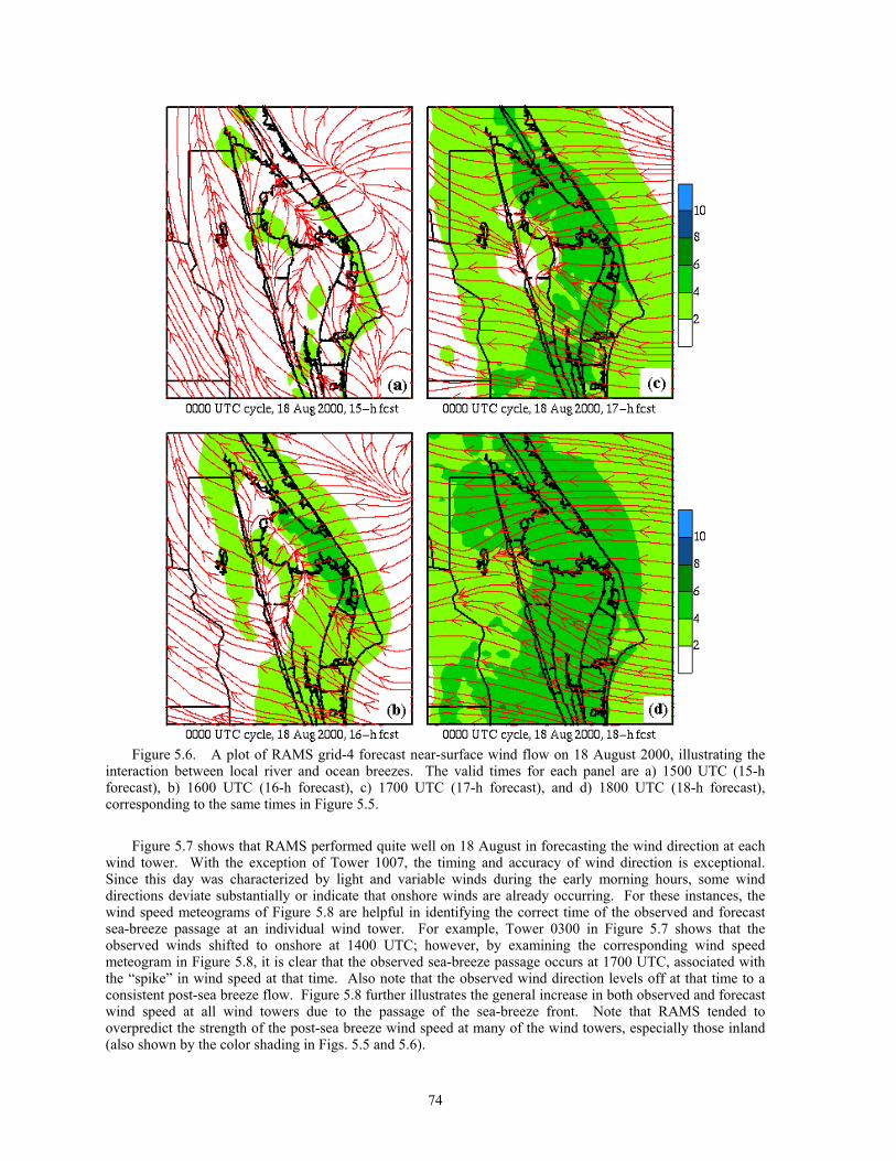
74

Figure 5.6. A plot of RAMS grid-4 forecast near-surface wind flow on 18 August 2000, illustrating the

interaction between local river and ocean breezes. The valid times for each panel are a) 1500 UTC (15-h forecast), b) 1600 UTC (16-h forecast), c) 1700 UTC (17-h forecast), and d) 1800 UTC (18-h forecast), corresponding to the same times in Figure 5.5.

Figure 5.7 shows that RAMS performed quite well on 18 August in forecasting the wind direction at each wind tower. With the exception of Tower 1007, the timing and accuracy of wind direction is exceptional. Since this day was characterized by light and variable winds during the early morning hours, some wind directions deviate substantially or indicate that onshore winds are already occurring. For these instances, the wind speed meteograms of Figure 5.8 are helpful in identifying the correct time of the observed and forecast sea-breeze passage at an individual wind tower. For example, Tower 0300 in Figure 5.7 shows that the observed winds shifted to onshore at 1400 UTC; however, by examining the corresponding wind speed meteogram in Figure 5.8, it is clear that the observed sea-breeze passage occurs at 1700 UTC, associated with the “spike” in wind speed at that time. Also note that the observed wind direction levels off at that time to a consistent post-sea breeze flow. Figure 5.8 further illustrates the general increase in both observed and forecast wind speed at all wind towers due to the passage of the sea-breeze front. Note that RAMS tended to overpredict the strength of the post-sea breeze wind speed at many of the wind towers, especially those inland (also shown by the color shading in Figs. 5.5 and 5.6).

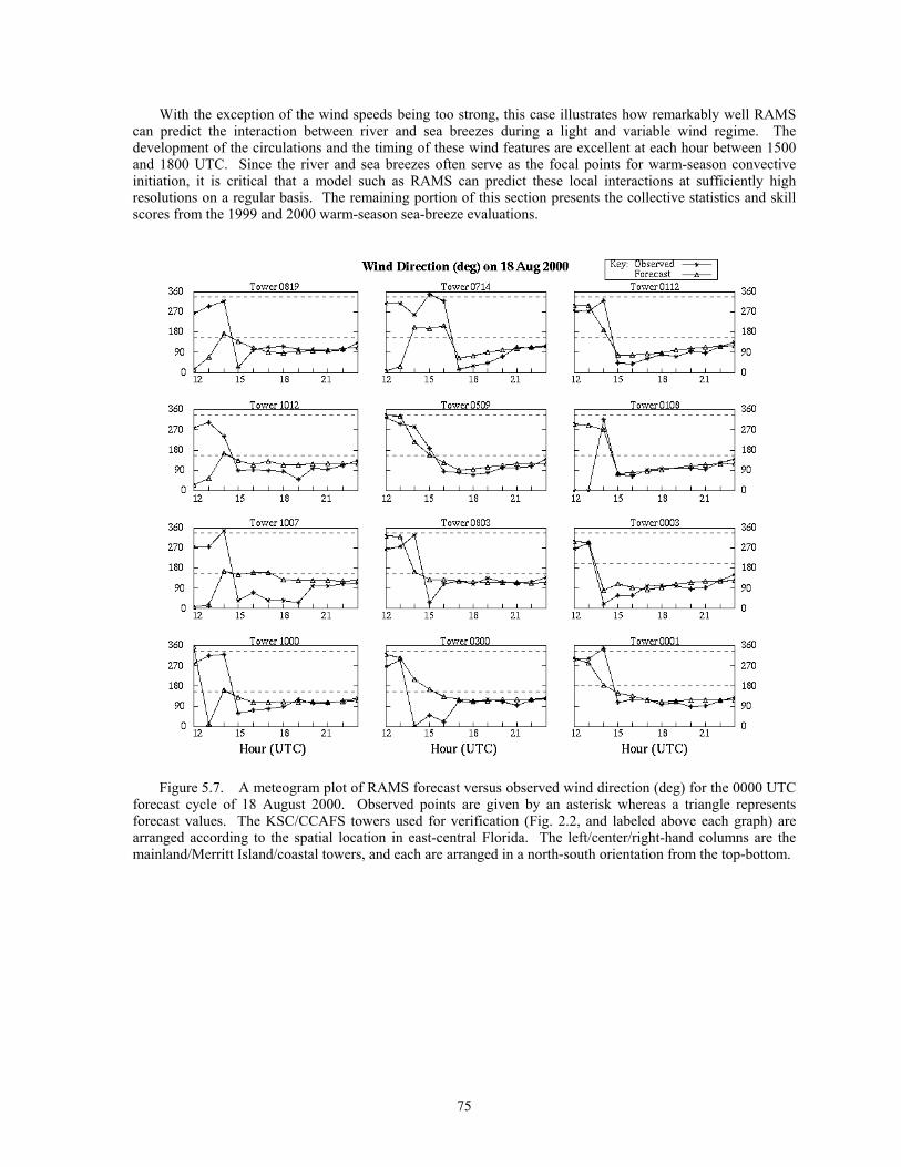
75

With the exception of the wind speeds being too strong, this case illustrates how remarkably well RAMS can predict the interaction between river and sea breezes during a light and variable wind regime. The development of the circulations and the timing of these wind features are excellent at each hour between 1500 and 1800 UTC. Since the river and sea breezes often serve as the focal points for warm-season convective initiation, it is critical that a model such as RAMS can predict these local interactions at sufficiently high resolutions on a regular basis. The remaining portion of this section presents the collective statistics and skill scores from the 1999 and 2000 warm-season sea-breeze evaluations.

Figure 5.7. A meteogram plot of RAMS forecast versus observed wind direction (deg) for the 0000 UTC

forecast cycle of 18 August 2000. Observed points are given by an asterisk whereas a triangle represents forecast values. The KSC/CCAFS towers used for verification (Fig. 2.2, and labeled above each graph) are arranged according to the spatial location in east-central Florida. The left/center/right-hand columns are the mainland/Merritt Island/coastal towers, and each are arranged in a north-south orientation from the top-bottom.

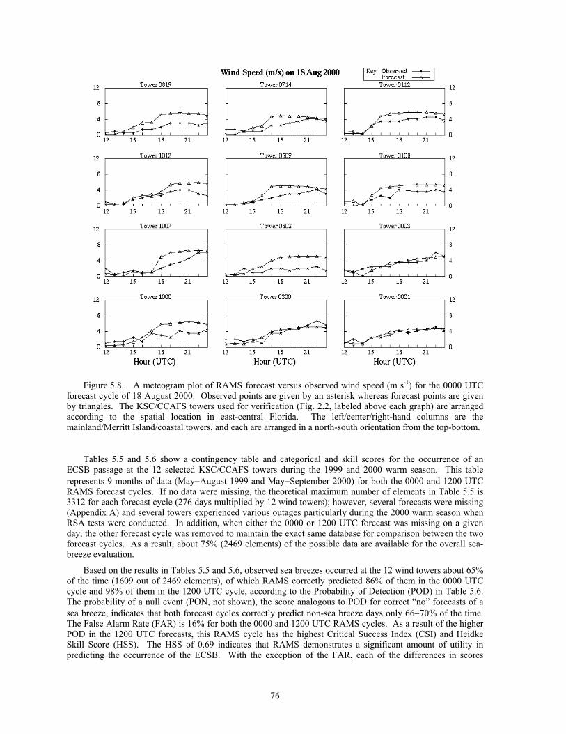
76

Figure 5.8. A meteogram plot of RAMS forecast versus observed wind speed (m s-1) for the 0000 UTC

forecast cycle of 18 August 2000. Observed points are given by an asterisk whereas forecast points are given by triangles. The KSC/CCAFS towers used for verification (Fig. 2.2, labeled above each graph) are arranged according to the spatial location in east-central Florida. The left/center/right-hand columns are the mainland/Merritt Island/coastal towers, and each are arranged in a north-south orientation from the top-bottom.

Tables 5.5 and 5.6 show a contingency table and categorical and skill scores for the occurrence of an ECSB passage at the 12 selected KSC/CCAFS towers during the 1999 and 2000 warm season. This table represents 9 months of data (May−August 1999 and May−September 2000) for both the 0000 and 1200 UTC RAMS forecast cycles. If no data were missing, the theoretical maximum number of elements in Table 5.5 is 3312 for each forecast cycle (276 days multiplied by 12 wind towers); however, several forecasts were missing (Appendix A) and several towers experienced various outages particularly during the 2000 warm season when RSA tests were conducted. In addition, when either the 0000 or 1200 UTC forecast was missing on a given day, the other forecast cycle was removed to maintain the exact same database for comparison between the two forecast cycles. As a result, about 75% (2469 elements) of the possible data are available for the overall sea-breeze evaluation.

Based on the results in Tables 5.5 and 5.6, observed sea breezes occurred at the 12 wind towers about 65% of the time (1609 out of 2469 elements), of which RAMS correctly predicted 86% of them in the 0000 UTC cycle and 98% of them in the 1200 UTC cycle, according to the Probability of Detection (POD) in Table 5.6. The probability of a null event (PON, not shown), the score analogous to POD for correct “no” forecasts of a sea breeze, indicates that both forecast cycles correctly predict non-sea breeze days only 66−70% of the time. The False Alarm Rate (FAR) is 16% for both the 0000 and 1200 UTC RAMS cycles. As a result of the higher POD in the 1200 UTC forecasts, this RAMS cycle has the highest Critical Success Index (CSI) and Heidke Skill Score (HSS). The HSS of 0.69 indicates that RAMS demonstrates a significant amount of utility in predicting the occurrence of the ECSB. With the exception of the FAR, each of the differences in scores

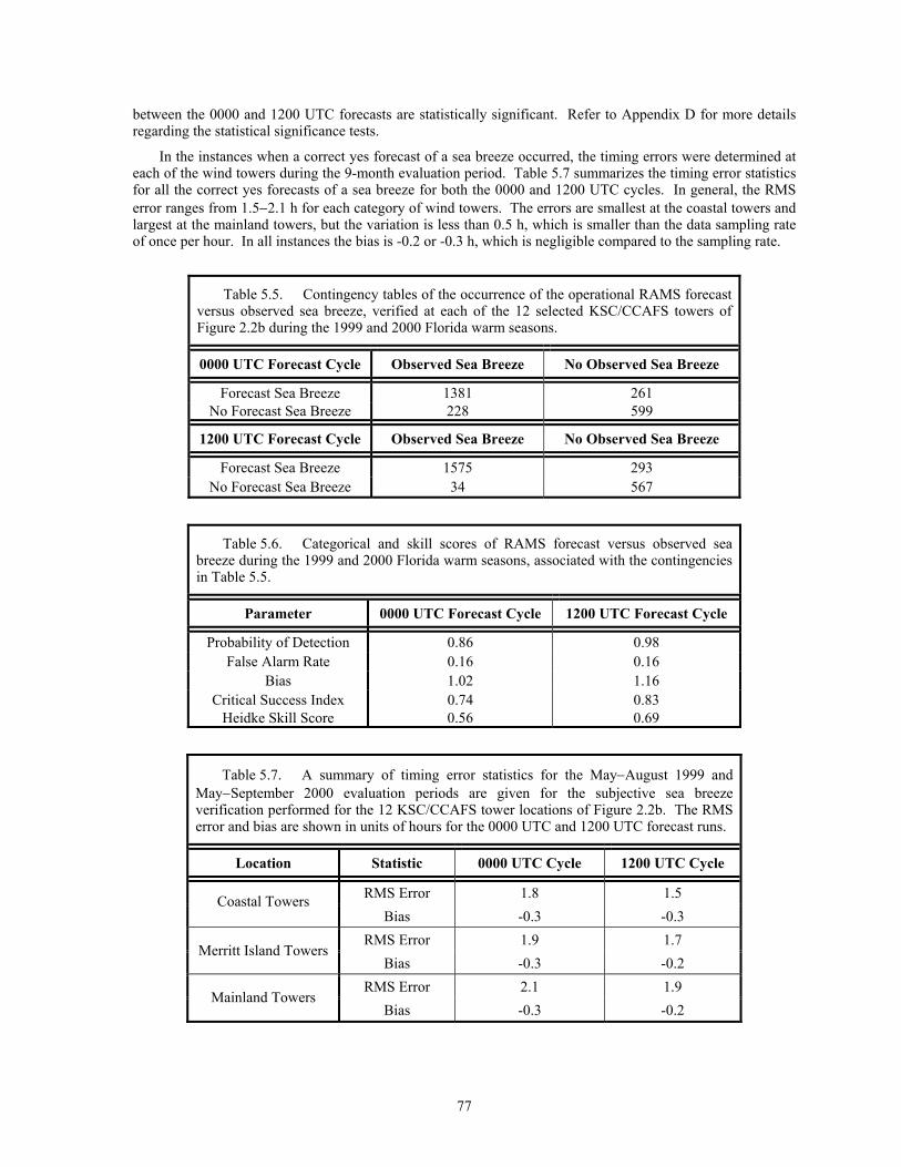
77

between the 0000 and 1200 UTC forecasts are statistically significant. Refer to Appendix D for more details regarding the statistical significance tests.

In the instances when a correct yes forecast of a sea breeze occurred, the timing errors were determined at each of the wind towers during the 9-month evaluation period. Table 5.7 summarizes the timing error statistics for all the correct yes forecasts of a sea breeze for both the 0000 and 1200 UTC cycles. In general, the RMS error ranges from 1.5−2.1 h for each category of wind towers. The errors are smallest at the coastal towers and largest at the mainland towers, but the variation is less than 0.5 h, which is smaller than the data sampling rate of once per hour. In all instances the bias is -0.2 or -0.3 h, which is negligible compared to the sampling rate.

Table 5.5. Contingency tables of the occurrence of the operational RAMS forecast versus observed sea breeze, verified at each of the 12 selected KSC/CCAFS towers of Figure 2.2b during the 1999 and 2000 Florida warm seasons.

0000 UTC Forecast Cycle Observed Sea Breeze No Observed Sea Breeze

Forecast Sea Breeze 1381 261 No Forecast Sea Breeze 228 599

1200 UTC Forecast Cycle Observed Sea Breeze No Observed Sea Breeze

Forecast Sea Breeze 1575 293 No Forecast Sea Breeze 34 567

Table 5.6. Categorical and skill scores of RAMS forecast versus observed sea breeze during the 1999 and 2000 Florida warm seasons, associated with the contingencies in Table 5.5.

Parameter 0000 UTC Forecast Cycle 1200 UTC Forecast Cycle

Probability of Detection 0.86 0.98 False Alarm Rate 0.16 0.16

Bias 1.02 1.16 Critical Success Index 0.74 0.83

Heidke Skill Score 0.56 0.69

Table 5.7. A summary of timing error statistics for the May−August 1999 and May−September 2000 evaluation periods are given for the subjective sea breeze verification performed for the 12 KSC/CCAFS tower locations of Figure 2.2b. The RMS error and bias are shown in units of hours for the 0000 UTC and 1200 UTC forecast runs.

Location Statistic 0000 UTC Cycle 1200 UTC Cycle

RMS Error 1.8 1.5 Coastal Towers Bias -0.3 -0.3

RMS Error 1.9 1.7 Merritt Island Towers

Bias -0.3 -0.2 RMS Error 2.1 1.9

Mainland Towers Bias -0.3 -0.2

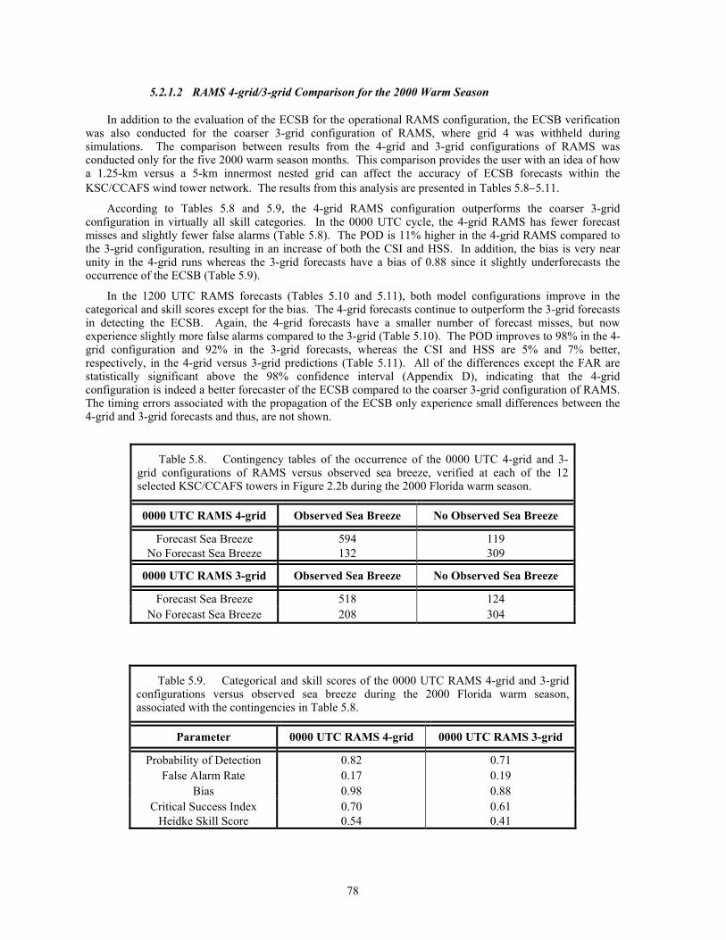
78

5.2.1.2 RAMS 4-grid/3-grid Comparison for the 2000 Warm Season

In addition to the evaluation of the ECSB for the operational RAMS configuration, the ECSB verification was also conducted for the coarser 3-grid configuration of RAMS, where grid 4 was withheld during simulations. The comparison between results from the 4-grid and 3-grid configurations of RAMS was conducted only for the five 2000 warm season months. This comparison provides the user with an idea of how a 1.25-km versus a 5-km innermost nested grid can affect the accuracy of ECSB forecasts within the KSC/CCAFS wind tower network. The results from this analysis are presented in Tables 5.8−5.11.

According to Tables 5.8 and 5.9, the 4-grid RAMS configuration outperforms the coarser 3-grid configuration in virtually all skill categories. In the 0000 UTC cycle, the 4-grid RAMS has fewer forecast misses and slightly fewer false alarms (Table 5.8). The POD is 11% higher in the 4-grid RAMS compared to the 3-grid configuration, resulting in an increase of both the CSI and HSS. In addition, the bias is very near unity in the 4-grid runs whereas the 3-grid forecasts have a bias of 0.88 since it slightly underforecasts the occurrence of the ECSB (Table 5.9).

In the 1200 UTC RAMS forecasts (Tables 5.10 and 5.11), both model configurations improve in the categorical and skill scores except for the bias. The 4-grid forecasts continue to outperform the 3-grid forecasts in detecting the ECSB. Again, the 4-grid forecasts have a smaller number of forecast misses, but now experience slightly more false alarms compared to the 3-grid (Table 5.10). The POD improves to 98% in the 4-grid configuration and 92% in the 3-grid forecasts, whereas the CSI and HSS are 5% and 7% better, respectively, in the 4-grid versus 3-grid predictions (Table 5.11). All of the differences except the FAR are statistically significant above the 98% confidence interval (Appendix D), indicating that the 4-grid configuration is indeed a better forecaster of the ECSB compared to the coarser 3-grid configuration of RAMS. The timing errors associated with the propagation of the ECSB only experience small differences between the 4-grid and 3-grid forecasts and thus, are not shown.

Table 5.8. Contingency tables of the occurrence of the 0000 UTC 4-grid and 3-grid configurations of RAMS versus observed sea breeze, verified at each of the 12 selected KSC/CCAFS towers in Figure 2.2b during the 2000 Florida warm season.

0000 UTC RAMS 4-grid Observed Sea Breeze No Observed Sea Breeze

Forecast Sea Breeze 594 119 No Forecast Sea Breeze 132 309

0000 UTC RAMS 3-grid Observed Sea Breeze No Observed Sea Breeze

Forecast Sea Breeze 518 124 No Forecast Sea Breeze 208 304

Table 5.9. Categorical and skill scores of the 0000 UTC RAMS 4-grid and 3-grid configurations versus observed sea breeze during the 2000 Florida warm season, associated with the contingencies in Table 5.8.

Parameter 0000 UTC RAMS 4-grid 0000 UTC RAMS 3-grid

Probability of Detection 0.82 0.71 False Alarm Rate 0.17 0.19

Bias 0.98 0.88 Critical Success Index 0.70 0.61

Heidke Skill Score 0.54 0.41

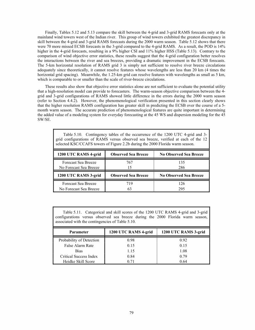
79

Finally, Tables 5.12 and 5.13 compare the skill between the 4-grid and 3-grid RAMS forecasts only at the mainland wind towers west of the Indian river. This group of wind towers exhibited the greatest discrepancy in skill between the 4-grid and 3-grid RAMS forecasts during the 2000 warm season. Table 5.12 shows that there were 70 more missed ECSB forecasts in the 3-grid compared to the 4-grid RAMS. As a result, the POD is 14% higher in the 4-grid forecasts, resulting in a 9% higher CSI and 11% higher HSS (Table 5.13). Contrary to the comparison of wind objective error statistics, these results suggest that the 4-grid configuration better resolves the interactions between the river and sea breezes, providing a dramatic improvement in the ECSB forecasts. The 5-km horizontal resolution of RAMS grid 3 is simply not sufficient to resolve river breeze circulations adequately since theoretically, it cannot resolve features whose wavelengths are less than 20 km (4 times the horizontal grid spacing). Meanwhile, the 1.25-km grid can resolve features with wavelengths as small as 5 km, which is comparable to or smaller than the scale of river-breeze circulations.

These results also show that objective error statistics alone are not sufficient to evaluate the potential utility that a high-resolution model can provide to forecasters. The warm-season objective comparison between the 4-grid and 3-grid configurations of RAMS showed little difference in the errors during the 2000 warm season (refer to Section 4.4.2). However, the phenomenological verification presented in this section clearly shows that the higher resolution RAMS configuration has greater skill in predicting the ECSB over the course of a 5-month warm season. The accurate prediction of phenomenological features are quite important in determining the added value of a modeling system for everyday forecasting at the 45 WS and dispersion modeling for the 45 SW/SE.

Table 5.10. Contingency tables of the occurrence of the 1200 UTC 4-grid and 3-grid configurations of RAMS versus observed sea breeze, verified at each of the 12 selected KSC/CCAFS towers of Figure 2.2b during the 2000 Florida warm season.

1200 UTC RAMS 4-grid Observed Sea Breeze No Observed Sea Breeze

Forecast Sea Breeze 767 135 No Forecast Sea Breeze 15 286

1200 UTC RAMS 3-grid Observed Sea Breeze No Observed Sea Breeze

Forecast Sea Breeze 719 126 No Forecast Sea Breeze 63 295

Table 5.11. Categorical and skill scores of the 1200 UTC RAMS 4-grid and 3-grid configurations versus observed sea breeze during the 2000 Florida warm season, associated with the contingencies of Table 5.10.

Parameter 1200 UTC RAMS 4-grid 1200 UTC RAMS 3-grid

Probability of Detection 0.98 0.92 False Alarm Rate 0.15 0.15

Bias 1.15 1.08 Critical Success Index 0.84 0.79

Heidke Skill Score 0.71 0.64

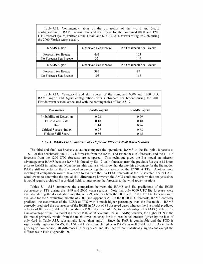
80

Table 5.12. Contingency tables of the occurrence of the 4-grid and 3-grid configurations of RAMS versus observed sea breeze for the combined 0000 and 1200 UTC forecast cycles, verified at the 4 mainland KSC/CCAFS towers of Figure 2.2b during the 2000 Florida warm season.

RAMS 4-grid Observed Sea Breeze No Observed Sea Breeze

Forecast Sea Breeze 463 103 No Forecast Sea Breeze 35 149

RAMS 3-grid Observed Sea Breeze No Observed Sea Breeze

Forecast Sea Breeze 393 84 No Forecast Sea Breeze 105 168

Table 5.13. Categorical and skill scores of the combined 0000 and 1200 UTC RAMS 4-grid and 3-grid configurations versus observed sea breeze during the 2000 Florida warm season, associated with the contingencies of Table 5.12.

Parameter RAMS 4-grid RAMS 3-grid

Probability of Detection 0.93 0.79 False Alarm Rate 0.18 0.18

Bias 1.14 0.96 Critical Success Index 0.77 0.68

Heidke Skill Score 0.56 0.45

5.2.1.3 RAMS/Eta Comparison at TTS for the 1999 and 2000 Warm Seasons

The third and final sea-breeze evaluation compares the operational RAMS to the Eta point forecasts at TTS. For this benchmark, the 13−23-h forecasts from the RAMS and Eta 0000 UTC forecasts, and the 1−11-h forecasts from the 1200 UTC forecasts are compared. This technique gives the Eta model an inherent advantage over RAMS because RAMS is forced by Eta 12−36-h forecasts from the previous Eta cycle 12 hours prior to RAMS initialization. Nonetheless, this analysis will show that despite this advantage for the Eta model, RAMS still outperforms the Eta model in predicting the occurrence of the ECSB at TTS. Another more meaningful comparison would have been to evaluate the Eta ECSB forecasts at the 12 selected KSC/CCAFS wind towers to determine the spatial skill differences; however, the AMU could not perform this analysis since it would require archived Eta gridded fields to interpolate the forecasts to the wind-tower locations.

Tables 5.14−5.17 summarize the comparison between the RAMS and Eta predictions of the ECSB occurrence at TTS during the 1999 and 2000 warm seasons. Note that only 0000 UTC Eta forecasts were available during the 4 evaluation months in 1999, whereas both the 0000 and 1200 UTC Eta forecasts were available for the 5 evaluation months of 2000 (see Appendix A). In the 0000 UTC forecasts, RAMS correctly predicted the occurrence of the ECSB at TTS with a much higher percentage than the Eta model. RAMS correctly predicted the occurrence of the ECSB in 73 out of 88 observed cases whereas the Eta model predicted only 47 of 88 cases (Table 5.14), yielding a POD difference of 30% to the advantage of RAMS (Table 5.15). One advantage of the Eta model is a better PON at 88% versus 78% in RAMS; however, the higher PON in the Eta model primarily results from the much lower tendency for it to predict sea breezes (given by the bias of only 0.61 in Table 5.15, substantially lower than unity). Since the FAR is comparable and the POD is significantly higher in RAMS, the CSI and HSS are much higher in RAMS as well (Table 5.15). As in the 4-grid/3-grid comparison, all differences in categorical and skill scores are statistically significant except the differences in FAR (Appendix D).

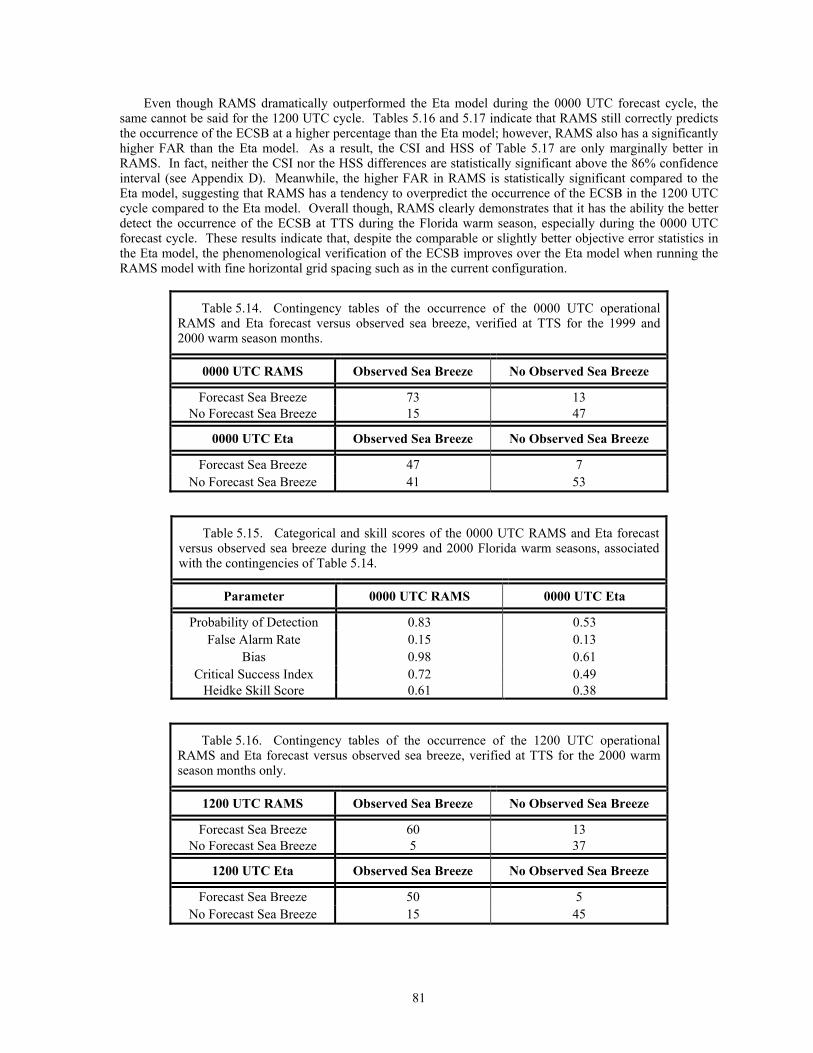
81

Even though RAMS dramatically outperformed the Eta model during the 0000 UTC forecast cycle, the same cannot be said for the 1200 UTC cycle. Tables 5.16 and 5.17 indicate that RAMS still correctly predicts the occurrence of the ECSB at a higher percentage than the Eta model; however, RAMS also has a significantly higher FAR than the Eta model. As a result, the CSI and HSS of Table 5.17 are only marginally better in RAMS. In fact, neither the CSI nor the HSS differences are statistically significant above the 86% confidence interval (see Appendix D). Meanwhile, the higher FAR in RAMS is statistically significant compared to the Eta model, suggesting that RAMS has a tendency to overpredict the occurrence of the ECSB in the 1200 UTC cycle compared to the Eta model. Overall though, RAMS clearly demonstrates that it has the ability the better detect the occurrence of the ECSB at TTS during the Florida warm season, especially during the 0000 UTC forecast cycle. These results indicate that, despite the comparable or slightly better objective error statistics in the Eta model, the phenomenological verification of the ECSB improves over the Eta model when running the RAMS model with fine horizontal grid spacing such as in the current configuration.

Table 5.14. Contingency tables of the occurrence of the 0000 UTC operational RAMS and Eta forecast versus observed sea breeze, verified at TTS for the 1999 and 2000 warm season months.

0000 UTC RAMS Observed Sea Breeze No Observed Sea Breeze

Forecast Sea Breeze 73 13 No Forecast Sea Breeze 15 47

0000 UTC Eta Observed Sea Breeze No Observed Sea Breeze

Forecast Sea Breeze 47 7 No Forecast Sea Breeze 41 53

Table 5.15. Categorical and skill scores of the 0000 UTC RAMS and Eta forecast versus observed sea breeze during the 1999 and 2000 Florida warm seasons, associated with the contingencies of Table 5.14.

Parameter 0000 UTC RAMS 0000 UTC Eta

Probability of Detection 0.83 0.53 False Alarm Rate 0.15 0.13

Bias 0.98 0.61 Critical Success Index 0.72 0.49

Heidke Skill Score 0.61 0.38

Table 5.16. Contingency tables of the occurrence of the 1200 UTC operational RAMS and Eta forecast versus observed sea breeze, verified at TTS for the 2000 warm season months only.

1200 UTC RAMS Observed Sea Breeze No Observed Sea Breeze

Forecast Sea Breeze 60 13 No Forecast Sea Breeze 5 37

1200 UTC Eta Observed Sea Breeze No Observed Sea Breeze

Forecast Sea Breeze 50 5 No Forecast Sea Breeze 15 45

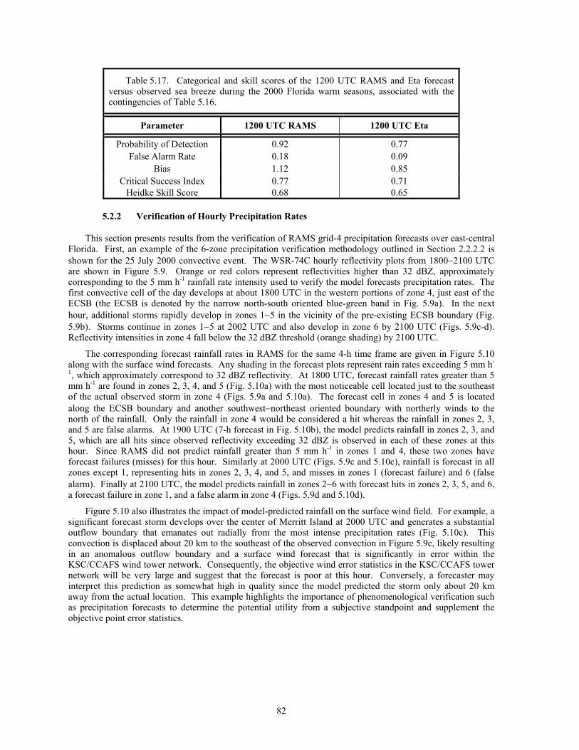
82

Table 5.17. Categorical and skill scores of the 1200 UTC RAMS and Eta forecast versus observed sea breeze during the 2000 Florida warm seasons, associated with the contingencies of Table 5.16.

Parameter 1200 UTC RAMS 1200 UTC Eta

Probability of Detection 0.92 0.77 False Alarm Rate 0.18 0.09

Bias 1.12 0.85 Critical Success Index 0.77 0.71

Heidke Skill Score 0.68 0.65

5.2.2 Verification of Hourly Precipitation Rates

This section presents results from the verification of RAMS grid-4 precipitation forecasts over east-central Florida. First, an example of the 6-zone precipitation verification methodology outlined in Section 2.2.2.2 is shown for the 25 July 2000 convective event. The WSR-74C hourly reflectivity plots from 1800−2100 UTC are shown in Figure 5.9. Orange or red colors represent reflectivities higher than 32 dBZ, approximately corresponding to the 5 mm h-1 rainfall rate intensity used to verify the model forecasts precipitation rates. The first convective cell of the day develops at about 1800 UTC in the western portions of zone 4, just east of the ECSB (the ECSB is denoted by the narrow north-south oriented blue-green band in Fig. 5.9a). In the next hour, additional storms rapidly develop in zones 1−5 in the vicinity of the pre-existing ECSB boundary (Fig. 5.9b). Storms continue in zones 1−5 at 2002 UTC and also develop in zone 6 by 2100 UTC (Figs. 5.9c-d). Reflectivity intensities in zone 4 fall below the 32 dBZ threshold (orange shading) by 2100 UTC.

The corresponding forecast rainfall rates in RAMS for the same 4-h time frame are given in Figure 5.10 along with the surface wind forecasts. Any shading in the forecast plots represent rain rates exceeding 5 mm h-

1, which approximately correspond to 32 dBZ reflectivity. At 1800 UTC, forecast rainfall rates greater than 5 mm h-1 are found in zones 2, 3, 4, and 5 (Fig. 5.10a) with the most noticeable cell located just to the southeast of the actual observed storm in zone 4 (Figs. 5.9a and 5.10a). The forecast cell in zones 4 and 5 is located along the ECSB boundary and another southwest−northeast oriented boundary with northerly winds to the north of the rainfall. Only the rainfall in zone 4 would be considered a hit whereas the rainfall in zones 2, 3, and 5 are false alarms. At 1900 UTC (7-h forecast in Fig. 5.10b), the model predicts rainfall in zones 2, 3, and 5, which are all hits since observed reflectivity exceeding 32 dBZ is observed in each of these zones at this hour. Since RAMS did not predict rainfall greater than 5 mm h-1 in zones 1 and 4, these two zones have forecast failures (misses) for this hour. Similarly at 2000 UTC (Figs. 5.9c and 5.10c), rainfall is forecast in all zones except 1, representing hits in zones 2, 3, 4, and 5, and misses in zones 1 (forecast failure) and 6 (false alarm). Finally at 2100 UTC, the model predicts rainfall in zones 2−6 with forecast hits in zones 2, 3, 5, and 6, a forecast failure in zone 1, and a false alarm in zone 4 (Figs. 5.9d and 5.10d).

Figure 5.10 also illustrates the impact of model-predicted rainfall on the surface wind field. For example, a significant forecast storm develops over the center of Merritt Island at 2000 UTC and generates a substantial outflow boundary that emanates out radially from the most intense precipitation rates (Fig. 5.10c). This convection is displaced about 20 km to the southeast of the observed convection in Figure 5.9c, likely resulting in an anomalous outflow boundary and a surface wind forecast that is significantly in error within the KSC/CCAFS wind tower network. Consequently, the objective wind error statistics in the KSC/CCAFS tower network will be very large and suggest that the forecast is poor at this hour. Conversely, a forecaster may interpret this prediction as somewhat high in quality since the model predicted the storm only about 20 km away from the actual location. This example highlights the importance of phenomenological verification such as precipitation forecasts to determine the potential utility from a subjective standpoint and supplement the objective point error statistics.

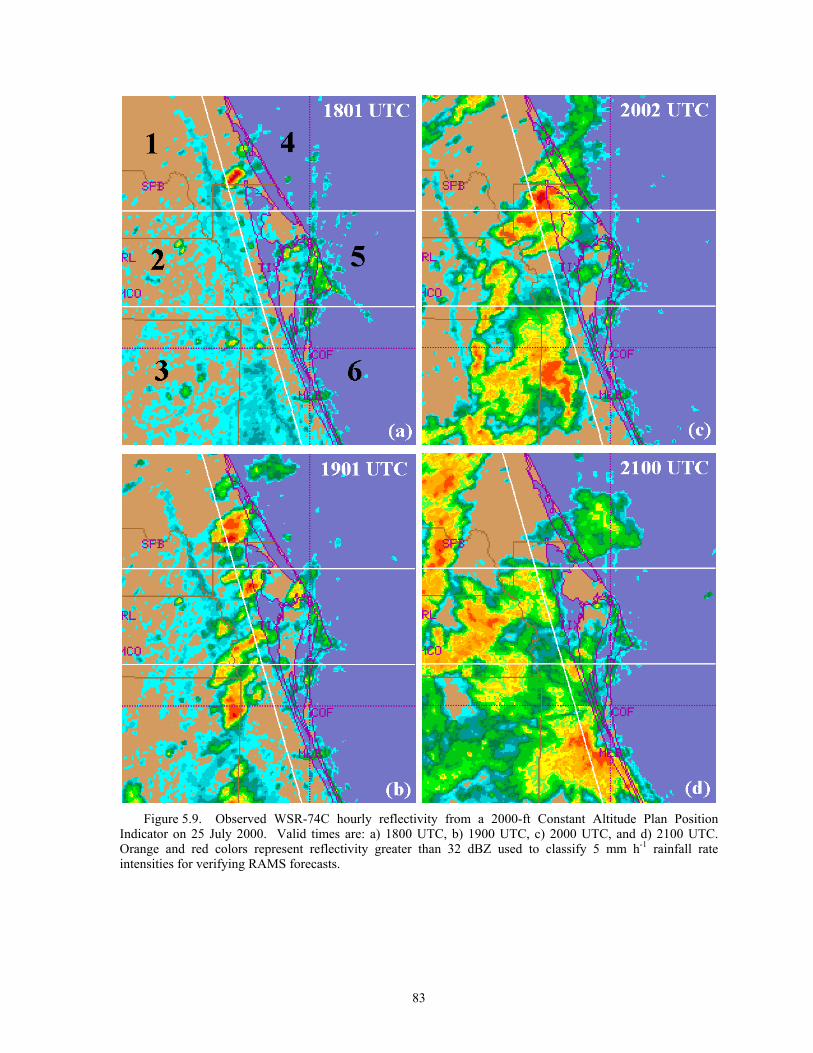
83

Figure 5.9. Observed WSR-74C hourly reflectivity from a 2000-ft Constant Altitude Plan Position

Indicator on 25 July 2000. Valid times are: a) 1800 UTC, b) 1900 UTC, c) 2000 UTC, and d) 2100 UTC. Orange and red colors represent reflectivity greater than 32 dBZ used to classify 5 mm h-1 rainfall rate intensities for verifying RAMS forecasts.

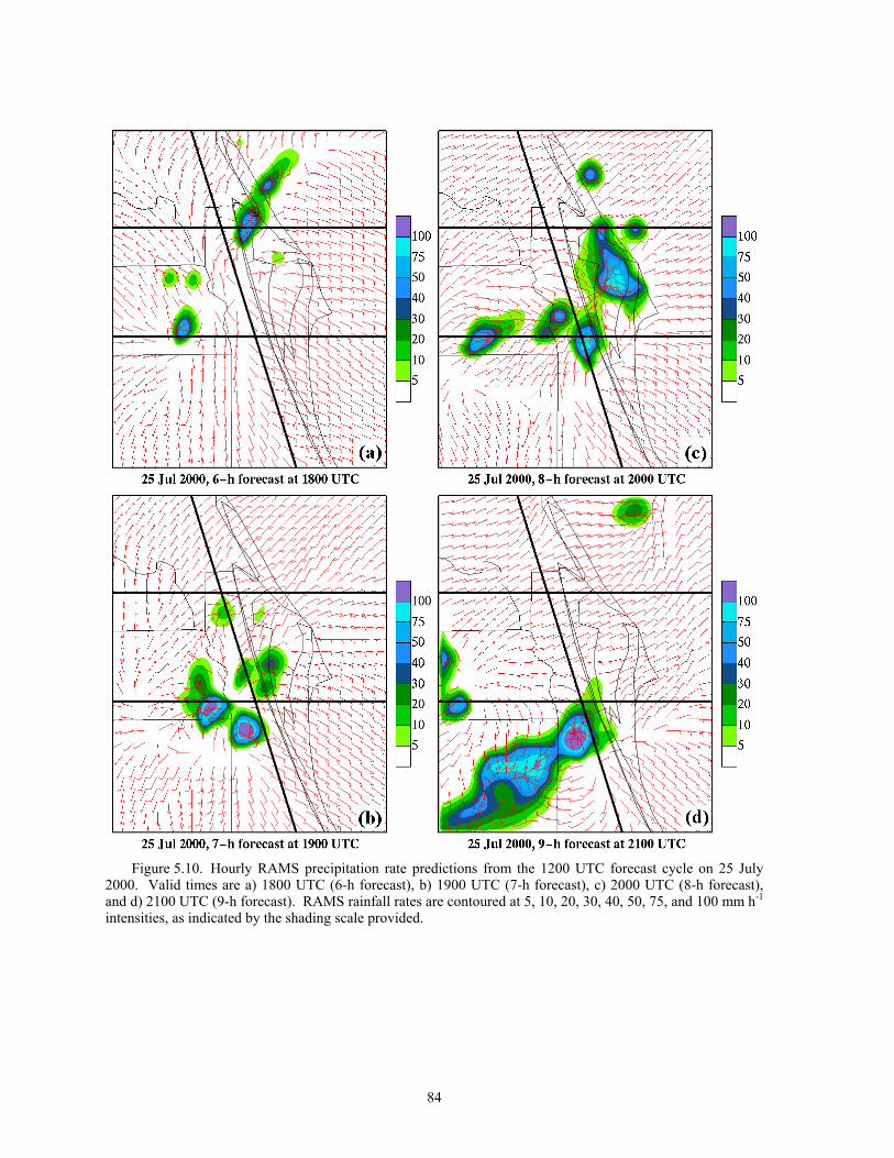
84

Figure 5.10. Hourly RAMS precipitation rate predictions from the 1200 UTC forecast cycle on 25 July

2000. Valid times are a) 1800 UTC (6-h forecast), b) 1900 UTC (7-h forecast), c) 2000 UTC (8-h forecast), and d) 2100 UTC (9-h forecast). RAMS rainfall rates are contoured at 5, 10, 20, 30, 40, 50, 75, and 100 mm h-1 intensities, as indicated by the shading scale provided.

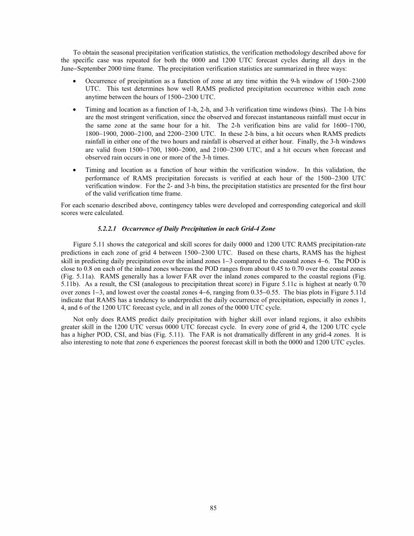
85

To obtain the seasonal precipitation verification statistics, the verification methodology described above for the specific case was repeated for both the 0000 and 1200 UTC forecast cycles during all days in the June−September 2000 time frame. The precipitation verification statistics are summarized in three ways:

• Occurrence of precipitation as a function of zone at any time within the 9-h window of 1500−2300 UTC. This test determines how well RAMS predicted precipitation occurrence within each zone anytime between the hours of 1500−2300 UTC.

• Timing and location as a function of 1-h, 2-h, and 3-h verification time windows (bins). The 1-h bins are the most stringent verification, since the observed and forecast instantaneous rainfall must occur in the same zone at the same hour for a hit. The 2-h verification bins are valid for 1600−1700, 1800−1900, 2000−2100, and 2200−2300 UTC. In these 2-h bins, a hit occurs when RAMS predicts rainfall in either one of the two hours and rainfall is observed at either hour. Finally, the 3-h windows are valid from 1500−1700, 1800−2000, and 2100−2300 UTC, and a hit occurs when forecast and observed rain occurs in one or more of the 3-h times.

• Timing and location as a function of hour within the verification window. In this validation, the performance of RAMS precipitation forecasts is verified at each hour of the 1500−2300 UTC verification window. For the 2- and 3-h bins, the precipitation statistics are presented for the first hour of the valid verification time frame.

For each scenario described above, contingency tables were developed and corresponding categorical and skill scores were calculated.

5.2.2.1 Occurrence of Daily Precipitation in each Grid-4 Zone

Figure 5.11 shows the categorical and skill scores for daily 0000 and 1200 UTC RAMS precipitation-rate predictions in each zone of grid 4 between 1500−2300 UTC. Based on these charts, RAMS has the highest skill in predicting daily precipitation over the inland zones 1−3 compared to the coastal zones 4−6. The POD is close to 0.8 on each of the inland zones whereas the POD ranges from about 0.45 to 0.70 over the coastal zones (Fig. 5.11a). RAMS generally has a lower FAR over the inland zones compared to the coastal regions (Fig. 5.11b). As a result, the CSI (analogous to precipitation threat score) in Figure 5.11c is highest at nearly 0.70 over zones 1−3, and lowest over the coastal zones 4−6, ranging from 0.35−0.55. The bias plots in Figure 5.11d indicate that RAMS has a tendency to underpredict the daily occurrence of precipitation, especially in zones 1, 4, and 6 of the 1200 UTC forecast cycle, and in all zones of the 0000 UTC cycle.

Not only does RAMS predict daily precipitation with higher skill over inland regions, it also exhibits greater skill in the 1200 UTC versus 0000 UTC forecast cycle. In every zone of grid 4, the 1200 UTC cycle has a higher POD, CSI, and bias (Fig. 5.11). The FAR is not dramatically different in any grid-4 zones. It is also interesting to note that zone 6 experiences the poorest forecast skill in both the 0000 and 1200 UTC cycles.

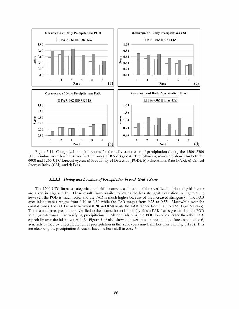
86

Occurrence of Daily Precipitation: POD

0.00

0.20

0.40

0.60

0.80

1.00

1 2 3 4 5 6Zone

Scor

e

POD-00Z POD-12Z

(a)

Occurrence of Daily Precipitation: CSI

0.00

0.20

0.40

0.60

0.80

1.00

1 2 3 4 5 6Zone

Scor

e

CSI-00Z CSI-12Z

(c)

Occurrence of Daily Precipitation: FAR

0.00

0.20

0.40

0.60

0.80

1.00

1 2 3 4 5 6Zone

Scor

e

FAR-00Z FAR-12Z

(b)

Occurrence of Daily Precipitation: Bias

0.40

0.70

1.00

1.30

1.60

1 2 3 4 5 6Zone

Scor

e

B ias-00Z Bias-12Z

(d) Figure 5.11. Categorical and skill scores for the daily occurrence of precipitation during the 1500−2300

UTC window in each of the 6 verification zones of RAMS grid 4. The following scores are shown for both the 0000 and 1200 UTC forecast cycles: a) Probability of Detection (POD), b) False Alarm Rate (FAR), c) Critical Success Index (CSI), and d) Bias.

5.2.2.2 Timing and Location of Precipitation in each Grid-4 Zone

The 1200 UTC forecast categorical and skill scores as a function of time verification bin and grid-4 zone are given in Figure 5.12. These results have similar trends as the less stringent evaluation in Figure 5.11; however, the POD is much lower and the FAR is much higher because of the increased stringency. The POD over inland zones ranges from 0.40 to 0.60 while the FAR ranges from 0.25 to 0.55. Meanwhile over the coastal zones, the POD is only between 0.20 and 0.50 while the FAR ranges from 0.40 to 0.65 (Figs. 5.12a-b). The instantaneous precipitation verified to the nearest hour (1-h bins) yields a FAR that is greater than the POD in all grid-4 zones. By verifying precipitation in 2-h and 3-h bins, the POD becomes larger than the FAR, especially over the inland zones 1−3. Figure 5.12 also shows the weakness in precipitation forecasts in zone 6, generally caused by underprediction of precipitation in this zone (bias much smaller than 1 in Fig. 5.12d). It is not clear why the precipitation forecasts have the least skill in zone 6.

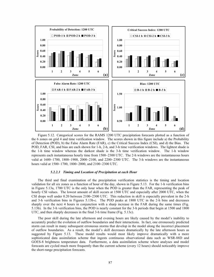
87

Probability of Detection: 1200 UTC

0.00

0.20

0.40

0.60

0.80

1.00

1 2 3 4 5 6Zone

Scor

ePOD-1 h POD-2 h POD-3 h

(a)

Critical Success Index: 1200 UTC

0.00

0.20

0.40

0.60

0.80

1.00

1 2 3 4 5 6Zone

Scor

e

CSI-1 h CSI-2 h CSI-3 h

(c)

False Alarm Rate: 1200 UTC

0.00

0.20

0.40

0.60

0.80

1.00

1 2 3 4 5 6Zone

Scor

e

FAR-1 h FAR-2 h FAR-3 h

(b)

Bias: 1200 UTC

0.50

1.00

1.50

1 2 3 4 5 6Zone

Scor

e

B-1 h B-2 h B-3 h

(d) Figure 5.12. Categorical scores for the RAMS 1200 UTC precipitation forecasts plotted as a function of

the 6 zones on grid 4 and time verification window. The scores shown in this figure include a) the Probability of Detection (POD), b) the False Alarm Rate (FAR), c) the Critical Success Index (CSI), and d) the Bias. The POD, FAR, CSI, and bias are each shown for 1-h, 2-h, and 3-h time verification windows. The lightest shade is the 1-h time window whereas the darkest shade is the 3-h time verification window. The 1-h window represents each instantaneous hourly time from 1500−2300 UTC. The 2-h windows are the instantaneous hours valid at 1600−1700, 1800−1900, 2000−2100, and 2200−2300 UTC. The 3-h windows are the instantaneous hours valid at 1500−1700, 1800−2000, and 2100−2300 UTC.

5.2.2.3 Timing and Location of Precipitation at each Hour

The third and final examination of the precipitation verification statistics is the timing and location validation for all six zones as a function of hour of the day, shown in Figure 5.13. For the 1-h verification bins in Figure 5.13a, 1700 UTC is the only hour when the POD is greater than the FAR, representing the peak of hourly CSI values. The lowest amount of skill occurs at 1500 UTC and especially after 2000 UTC, when the CSI drops well under 0.20 between 2100−2300 UTC. This reduction in skill is especially prevalent in the 2-h and 3-h verification bins in Figures 5.13b-c. The POD peaks at 1800 UTC in the 2-h bins and decreases sharply over the next 4 hours in conjunction with a sharp increase in the FAR during the same times (Fig. 5.13b). In the 3-h verification bins, the POD is nearly constant for the 3-h periods that begin at 1500 and 1800 UTC, and then sharply decreases in the final 3-h time frame (Fig. 5.13c).

The poor skill during the late afternoon and evening hours are likely caused by the model’s inability to accurately predict the evolution of outflow boundaries and their interactions. In fact, one erroneously predicted storm can result in many subsequent erroneous storms that develop in the model along the incorrect placement of outflow boundaries. As a result, the model’s skill decreases dramatically by the late afternoon hours as suggested by Figure 5.13. These model results would most likely improve dramatically with a more sophisticated data assimilation scheme that ingests continuous observational data such as WSR-88D and GOES-8 brightness temperature data. Furthermore, a data assimilation scheme where analyses and model forecasts are cycled much more frequently than the current scheme (every 12 hours) should noticeably improve the short-range precipitation forecasts.

88

Categorical Scores: 1200 UTC1-Hour Verification bins

0.00

0.20

0.40

0.60

0.80

1.00

15 16 17 18 19 20 21 22 23Hour (UTC)

Scor

e

POD FAR CSI

(a)

Categorical/Skill Scores: 1200 UTC2-Hour Verification bins

0.00

0.20

0.40

0.60

0.80

1.00

16 18 20 22Hour (UTC)

Scor

e

POD FAR CSI

(b)

Categorical/Skill Scores: 1200 UTC3-Hour Verification bins

0

0.2

0.4

0.6

0.8

1

15 18 21Hour (UTC)

Scor

e

POD FAR CSI

(c)

Figure 5.13. Categorical scores of RAMS 1200 UTC precipitation forecasts as a function of time of day for the a) 1-h time verification window, b) 2-h time verification window, and c) 3-h time verification window. The 1-h window represents each instantaneous hourly time from 1500 UTC to 2300 UTC. The 2-h windows are the instantaneous hours valid at 1600−1700, 1800−1900, 2000−2100, and 2200−2300 UTC. The 3-h windows are the instantaneous hours valid at 1500−1700, 1800−2000, and 2100−2300 UTC.

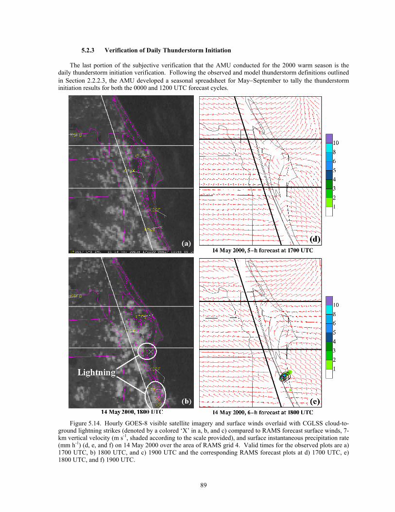
89

5.2.3 Verification of Daily Thunderstorm Initiation

The last portion of the subjective verification that the AMU conducted for the 2000 warm season is the daily thunderstorm initiation verification. Following the observed and model thunderstorm definitions outlined in Section 2.2.2.3, the AMU developed a seasonal spreadsheet for May−September to tally the thunderstorm initiation results for both the 0000 and 1200 UTC forecast cycles.

Figure 5.14. Hourly GOES-8 visible satellite imagery and surface winds overlaid with CGLSS cloud-to-

ground lightning strikes (denoted by a colored ‘X’ in a, b, and c) compared to RAMS forecast surface winds, 7-km vertical velocity (m s-1, shaded according to the scale provided), and surface instantaneous precipitation rate (mm h-1) (d, e, and f) on 14 May 2000 over the area of RAMS grid 4. Valid times for the observed plots are a) 1700 UTC, b) 1800 UTC, and c) 1900 UTC and the corresponding RAMS forecast plots at d) 1700 UTC, e) 1800 UTC, and f) 1900 UTC.

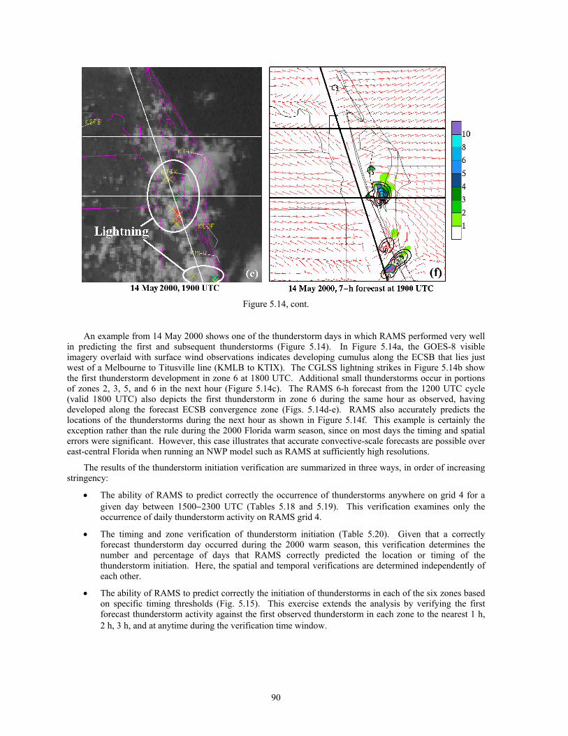
90

Figure 5.14, cont.

An example from 14 May 2000 shows one of the thunderstorm days in which RAMS performed very well in predicting the first and subsequent thunderstorms (Figure 5.14). In Figure 5.14a, the GOES-8 visible imagery overlaid with surface wind observations indicates developing cumulus along the ECSB that lies just west of a Melbourne to Titusville line (KMLB to KTIX). The CGLSS lightning strikes in Figure 5.14b show the first thunderstorm development in zone 6 at 1800 UTC. Additional small thunderstorms occur in portions of zones 2, 3, 5, and 6 in the next hour (Figure 5.14c). The RAMS 6-h forecast from the 1200 UTC cycle (valid 1800 UTC) also depicts the first thunderstorm in zone 6 during the same hour as observed, having developed along the forecast ECSB convergence zone (Figs. 5.14d-e). RAMS also accurately predicts the locations of the thunderstorms during the next hour as shown in Figure 5.14f. This example is certainly the exception rather than the rule during the 2000 Florida warm season, since on most days the timing and spatial errors were significant. However, this case illustrates that accurate convective-scale forecasts are possible over east-central Florida when running an NWP model such as RAMS at sufficiently high resolutions.

The results of the thunderstorm initiation verification are summarized in three ways, in order of increasing stringency:

• The ability of RAMS to predict correctly the occurrence of thunderstorms anywhere on grid 4 for a given day between 1500−2300 UTC (Tables 5.18 and 5.19). This verification examines only the occurrence of daily thunderstorm activity on RAMS grid 4.

• The timing and zone verification of thunderstorm initiation (Table 5.20). Given that a correctly forecast thunderstorm day occurred during the 2000 warm season, this verification determines the number and percentage of days that RAMS correctly predicted the location or timing of the thunderstorm initiation. Here, the spatial and temporal verifications are determined independently of each other.

• The ability of RAMS to predict correctly the initiation of thunderstorms in each of the six zones based on specific timing thresholds (Fig. 5.15). This exercise extends the analysis by verifying the first forecast thunderstorm activity against the first observed thunderstorm in each zone to the nearest 1 h, 2 h, 3 h, and at anytime during the verification time window.

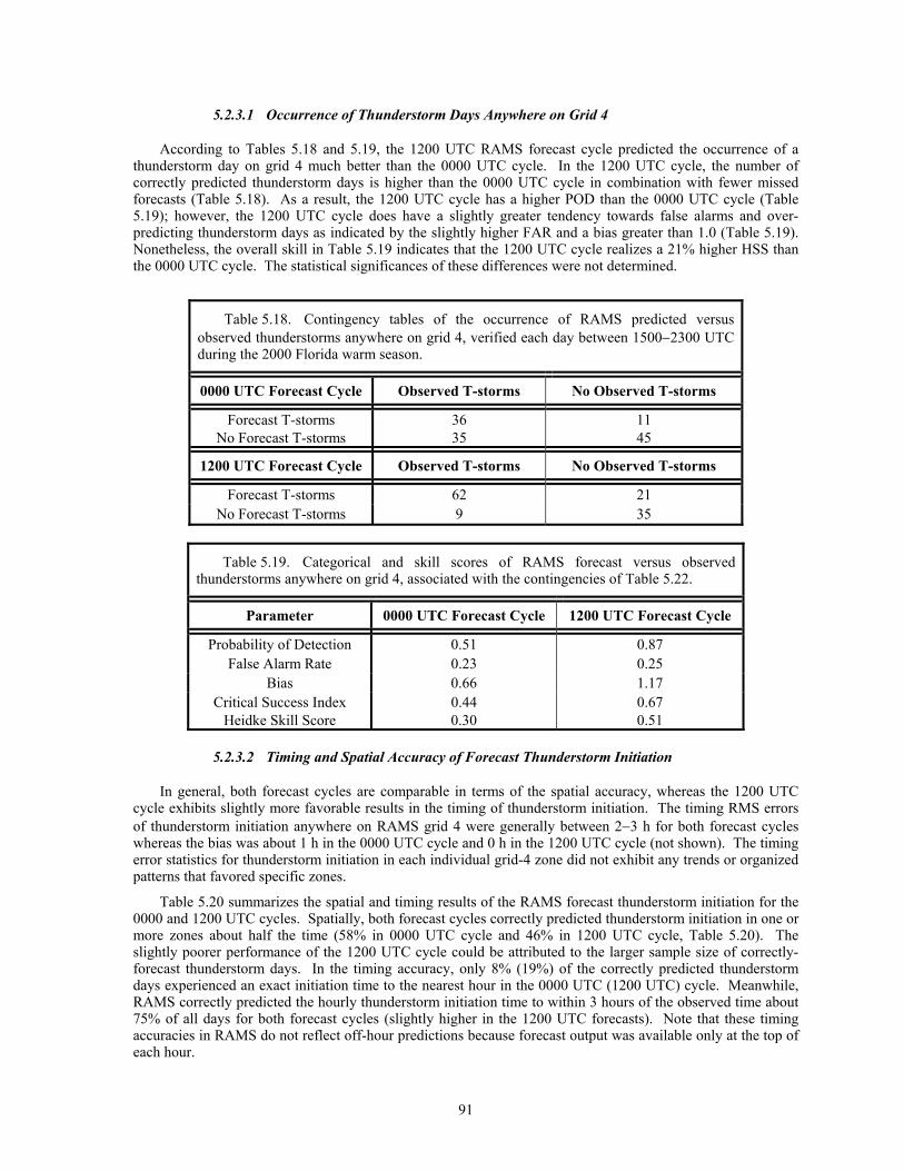
91

5.2.3.1 Occurrence of Thunderstorm Days Anywhere on Grid 4

According to Tables 5.18 and 5.19, the 1200 UTC RAMS forecast cycle predicted the occurrence of a thunderstorm day on grid 4 much better than the 0000 UTC cycle. In the 1200 UTC cycle, the number of correctly predicted thunderstorm days is higher than the 0000 UTC cycle in combination with fewer missed forecasts (Table 5.18). As a result, the 1200 UTC cycle has a higher POD than the 0000 UTC cycle (Table 5.19); however, the 1200 UTC cycle does have a slightly greater tendency towards false alarms and over-predicting thunderstorm days as indicated by the slightly higher FAR and a bias greater than 1.0 (Table 5.19). Nonetheless, the overall skill in Table 5.19 indicates that the 1200 UTC cycle realizes a 21% higher HSS than the 0000 UTC cycle. The statistical significances of these differences were not determined.

Table 5.18. Contingency tables of the occurrence of RAMS predicted versus observed thunderstorms anywhere on grid 4, verified each day between 1500−2300 UTC during the 2000 Florida warm season.

0000 UTC Forecast Cycle Observed T-storms No Observed T-storms

Forecast T-storms 36 11 No Forecast T-storms 35 45

1200 UTC Forecast Cycle Observed T-storms No Observed T-storms

Forecast T-storms 62 21 No Forecast T-storms 9 35

Table 5.19. Categorical and skill scores of RAMS forecast versus observed thunderstorms anywhere on grid 4, associated with the contingencies of Table 5.22.

Parameter 0000 UTC Forecast Cycle 1200 UTC Forecast Cycle

Probability of Detection 0.51 0.87 False Alarm Rate 0.23 0.25

Bias 0.66 1.17 Critical Success Index 0.44 0.67

Heidke Skill Score 0.30 0.51

5.2.3.2 Timing and Spatial Accuracy of Forecast Thunderstorm Initiation

In general, both forecast cycles are comparable in terms of the spatial accuracy, whereas the 1200 UTC cycle exhibits slightly more favorable results in the timing of thunderstorm initiation. The timing RMS errors of thunderstorm initiation anywhere on RAMS grid 4 were generally between 2−3 h for both forecast cycles whereas the bias was about 1 h in the 0000 UTC cycle and 0 h in the 1200 UTC cycle (not shown). The timing error statistics for thunderstorm initiation in each individual grid-4 zone did not exhibit any trends or organized patterns that favored specific zones.

Table 5.20 summarizes the spatial and timing results of the RAMS forecast thunderstorm initiation for the 0000 and 1200 UTC cycles. Spatially, both forecast cycles correctly predicted thunderstorm initiation in one or more zones about half the time (58% in 0000 UTC cycle and 46% in 1200 UTC cycle, Table 5.20). The slightly poorer performance of the 1200 UTC cycle could be attributed to the larger sample size of correctly-forecast thunderstorm days. In the timing accuracy, only 8% (19%) of the correctly predicted thunderstorm days experienced an exact initiation time to the nearest hour in the 0000 UTC (1200 UTC) cycle. Meanwhile, RAMS correctly predicted the hourly thunderstorm initiation time to within 3 hours of the observed time about 75% of all days for both forecast cycles (slightly higher in the 1200 UTC forecasts). Note that these timing accuracies in RAMS do not reflect off-hour predictions because forecast output was available only at the top of each hour.

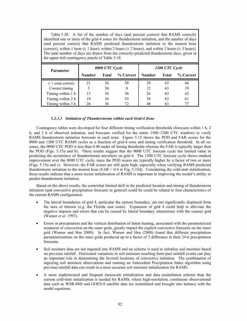
92

Table 5.20. A list of the number of days (and percent correct) that RAMS correctly identified one or more of the grid-4 zones for thunderstorm initiation, and the number of days (and percent correct) that RAMS predicted thunderstorm initiation to the nearest hour (correct), within 1 hour (± 1 hour), within 2 hours (± 2 hours), and within 3 hours (± 3 hours). The total number of days are drawn from the correctly-predicted thunderstorm days, given in the upper-left contingency panels of Table 5.18.

0000 UTC Cycle 1200 UTC Cycle Parameter

Number Total % Correct Number Total % Correct

≥ 1 zone correct 21 36 58 29 63 46 Correct timing 3 36 8 12 63 19

Timing within 1 h 13 36 36 26 63 42 Timing within 2 h 19 36 53 38 63 61 Timing within 3 h 26 36 72 48 63 77

5.2.3.3 Initiation of Thunderstorms within each Grid-4 Zone

Contingency tables were developed for four different timing verification thresholds (forecasts within 1 h, 2 h, and 3 h of observed initiation, and forecasts verified for the entire 1500−2300 UTC window) to verify RAMS thunderstorm initiation forecasts in each zone. Figure 5.15 shows the POD and FAR scores for the 0000 and 1200 UTC RAMS cycles as a function of grid-4 zone and timing verification threshold. In all six zones, the 0000 UTC POD is less than 0.40 under all timing thresholds whereas the FAR is typically larger than the POD (Figs. 5.15a and b). These results suggest that the 0000 UTC forecast cycle has limited value in predicting the occurrence of thunderstorms anywhere on grid 4. The 1200 UTC forecast cycle shows marked improvement over the 0000 UTC cycle, since the POD scores are typically higher by a factor of two or more (Figs. 5.15a and c). However, the FAR scores are still quite high, especially when verifying RAMS predicted thunderstorm initiation to the nearest hour (FAR > 0.4 in Fig. 5.15d). Considering the cold-start initialization, these results indicate that a more recent initialization of RAMS is important in improving the model’s ability to predict thunderstorm initiation.

Based on the above results, the somewhat limited skill in the predicted location and timing of thunderstorm initiation (and convective precipitation forecasts in general) could be could be related to four characteristics of the current RAMS configuration:

• The lateral boundaries of grid 4, particular the eastern boundary, are not significantly displaced from the area of interest (e.g. the Florida east coast). Expansion of grid 4 could help to alleviate the negative impacts and errors that can be caused by lateral boundary interactions with the coarser grid (Warner et al. 1997).

• Errors in precipitation and the vertical distribution of latent heating, associated with the parameterized treatment of convection on the outer grids, greatly impact the explicit convective forecasts on the inner grid (Warner and Hsu 2000). In fact, Warner and Hsu (2000) found that different precipitation parameterizations on the outer grids produced up to a factor of 3 difference in their 24-h precipitation forecasts.

• Soil moisture data are not ingested into RAMS and no scheme is used to initialize soil moisture based on previous rainfall. Horizontal variations in soil moisture resulting from past rainfall events can play an important role in determining the favored locations of convective initiation. The combination of ingesting soil moisture observations and running an Antecedent Precipitation Index algorithm using previous rainfall data can result in a more accurate soil moisture initialization for RAMS.

• A more sophisticated and frequent mesoscale initialization and data assimilation scheme than the current cold-start initialization is needed for RAMS, where high-resolution, continuous observational data such as WSR-88D and GOES-8 satellite data are assimilated and brought into balance with the model equations.

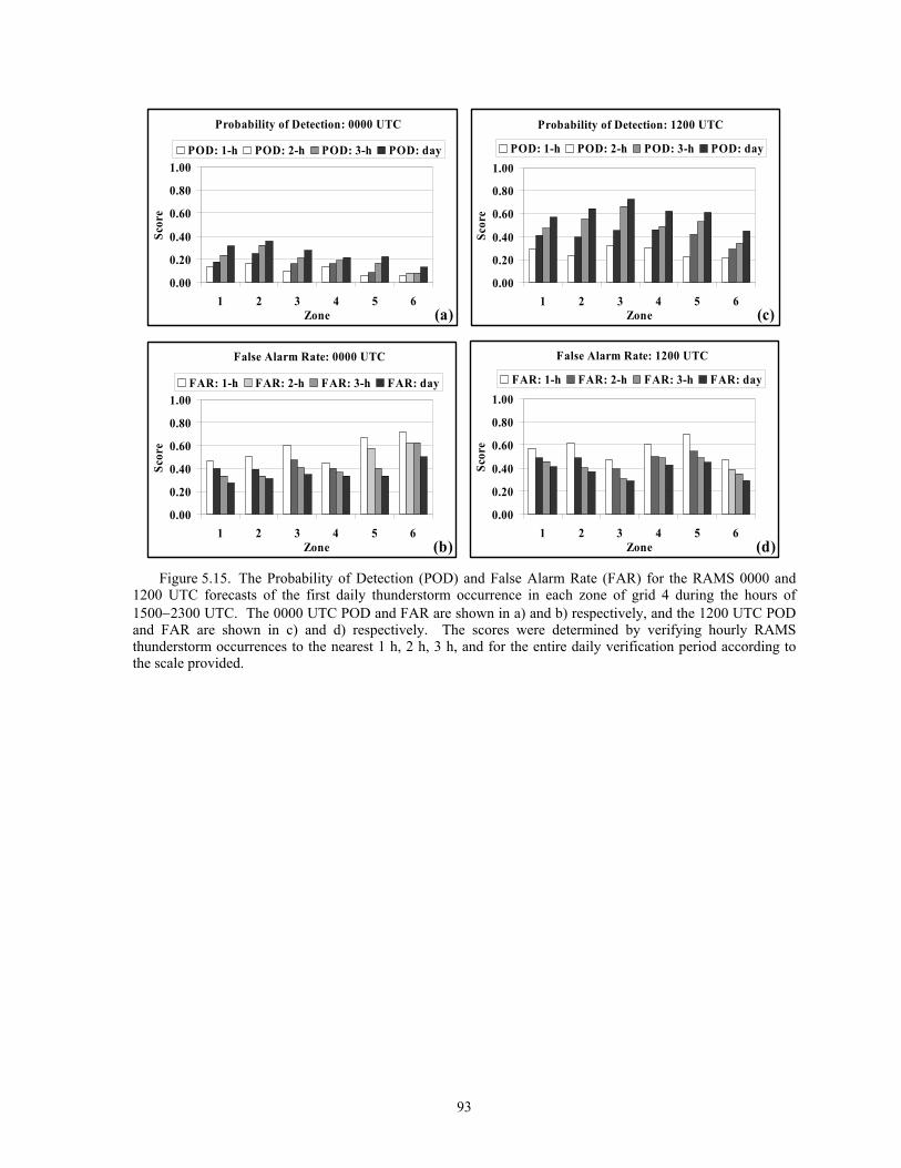
93

Probability of Detection: 0000 UTC

0.00

0.20

0.40

0.60

0.80

1.00

1 2 3 4 5 6Zone

Scor

ePOD: 1-h POD: 2-h POD: 3-h POD: day

(a)

Probability of Detection: 1200 UTC

0.00

0.20

0.40

0.60

0.80

1.00

1 2 3 4 5 6Zone

Scor

e

POD: 1-h POD: 2-h POD: 3-h POD: day

(c)

False Alarm Rate: 0000 UTC

0.00

0.20

0.40

0.60

0.80

1.00

1 2 3 4 5 6Zone

Scor

e

FAR: 1-h FAR: 2-h FAR: 3-h FAR: day

(b)

False Alarm Rate: 1200 UTC

0.00

0.20

0.40

0.60

0.80

1.00

1 2 3 4 5 6Zone

Scor

e

FAR: 1-h FAR: 2-h FAR: 3-h FAR: day

(d) Figure 5.15. The Probability of Detection (POD) and False Alarm Rate (FAR) for the RAMS 0000 and

1200 UTC forecasts of the first daily thunderstorm occurrence in each zone of grid 4 during the hours of 1500−2300 UTC. The 0000 UTC POD and FAR are shown in a) and b) respectively, and the 1200 UTC POD and FAR are shown in c) and d) respectively. The scores were determined by verifying hourly RAMS thunderstorm occurrences to the nearest 1 h, 2 h, 3 h, and for the entire daily verification period according to the scale provided.

94

6. Sensitivity Experiments in ERDAS RAMS Extension Task

This section presents results from selected sensitivity experiments designed to understand and possibly isolate the cause(s) of some of the RAMS forecast errors. In particular, these experiments strive to isolate the cause(s) of the low-level cold temperature bias that occurs during all seasons in RAMS.

6.1 Eta 0-h Forecasts as Background Field

This sensitivity test involved running 24-h forecasts of the full 4-grid configuration of RAMS using the most recent Eta 0-h rather than 12-h forecasts as a background fields for the RAMS initial condition. In addition, 0−24-h forecasts from the most recent Eta model were used as boundary conditions rather than the 12−36-h Eta forecasts. This experiment was run to determine if using more recent Eta forecasts would have any impact on the subsequent RAMS point forecast errors. A complete 4-grid experimental RAMS 24-h forecast could be completed in a little more than 24 h, given the limitations of the experimental hardware. As a result, every third RAMS initialization cycle was run for this experiment in order to collect a database of forecasts from both the 0000 and 1200 UTC cycles. The experiment was conducted from late March to the end of September 2000 in order to obtain a sufficiently large sample size for both the 0000 and 1200 UTC forecast cycles. The point error statistics from these experimental model runs were compiled and compared to the original RAMS forecasts using Eta 12-h forecasts as background fields (and 12−36-h Eta forecasts as boundary conditions).

In general, very little change occurred in the errors when using more recent Eta model output in the RAMS initial condition. Figures 6.1 and 6.2 show the 1200 UTC RAMS cycle point error statistics for the KSC/CCAFS wind-tower network, computed at 1.8 m for temperature and 16.5 m for wind direction. Both the operational (4-oper) and experimental (4-exp.) RAMS forecasts have RMS errors between 1.5 and 4.0°C during the course of the 24-h forecast (Figure 6.1b). In addition, the biases are nearly identical in magnitude for all forecast hours, with both RAMS forecasts demonstrating a daytime cold bias near -2°C between forecast hours 3 and 12 (Figure 6.1c). The most variation between 4-oper and 4-exp. occurs in the error standard deviation where a 0.5−1.0°C difference occurs between forecast hours 6 and 18, but favoring neither configuration.

In addition to the negligible changes in surface temperature errors, only minor differences are evident in wind-direction errors as well. The wind-direction RMS errors of 4-oper and 4-exp. are generally within 5−10° of each other during all 24 forecast hours (Figure 6.2a). The most significant difference occurs in the wind-direction bias, where the 4-exp. forecasts have a more negative bias compared to 4-oper, especially between forecast hours 3 and 9 (Figure 6.2b). However, the magnitude of these bias differences is inconsequential compared to the overall model errors, given by the RMS error.

Based on the surface point error results at the KSC/CCAFS wind-tower network, it appears that the more recent Eta background fields and boundary conditions do not substantially change or improve the RAMS point error statistics on the innermost grid 4. This small change in errors may be a result of the time frame used in this study. Most of the forecasts for this study were run during the 2000 Florida warm season (May−September) and large-scale meteorological regimes may not have played a substantial role in governing the RAMS errors. Nonetheless, the results of this sensitivity experiment are important because the surface errors demonstrate that using a more up-to-date background field does not likely improve the surface model errors on RAMS grid 4.

6.2 Change of Radiation Scheme

Another sensitivity experiment conducted by the AMU was running RAMS with a different radiation scheme and monitoring the impacts on the surface temperature fields. In this instance, the Mahrer and Pielke (1977) radiation scheme is used instead of the Chen and Cotton (1988) scheme. Mahrer/Pielke (MP) is a simplified radiation parameterization in which the effects of clouds do not impact the incoming solar radiation heating term. Each forecast was run for the 19 April 1999 0000 UTC forecast when a substantial surface-based cold bias occurred. The results of this experiment proved to be quite interesting. The MP run had a reduced daytime cold temperature bias at the surface compared to the operational RAMS configuration using Chen and

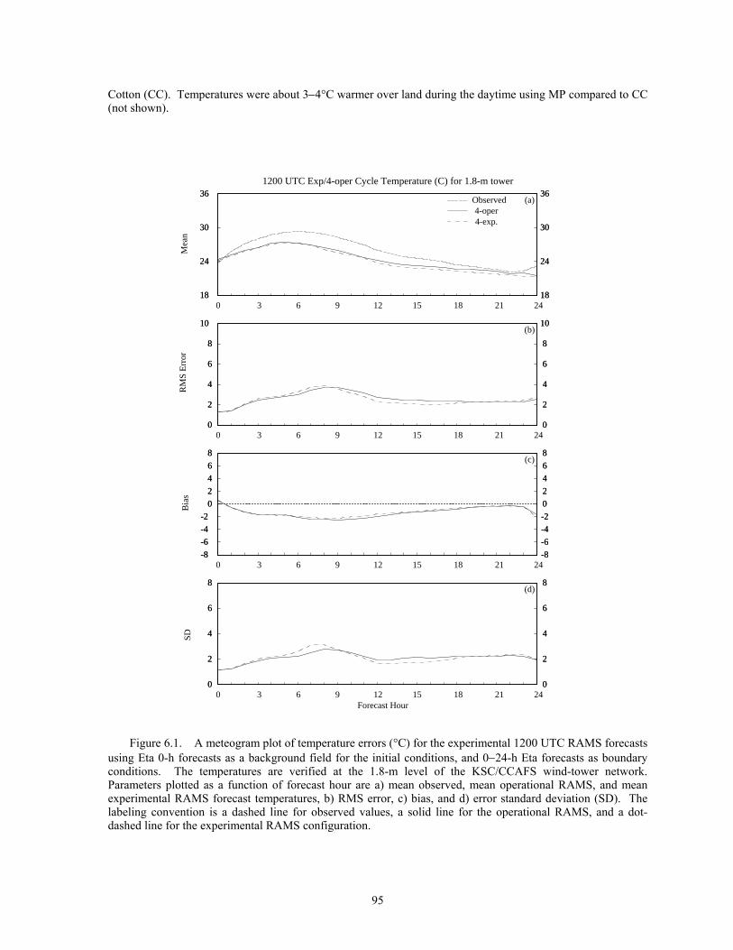
95

Cotton (CC). Temperatures were about 3−4°C warmer over land during the daytime using MP compared to CC (not shown).

18

24

30

36

18

24

30

36

0

2

4

6

8

10

0

2

4

6

8

10

-8

-6

-4

-2

0

2

4

6

8

-8

-6

-4

-2

0

2

4

6

8

10/00 10/02 10/04 10/06 10/08 10/10 10/12 10/14 10/16 10/18 10/20 10/22 11/000

2

4

6

8

0

2

4

6

8

18

24

30

36

18

24

30

36

0

2

4

6

8

10

0

2

4

6

8

10

-8

-6

-4

-2

0

2

4

6

8

-8

-6

-4

-2

0

2

4

6

8

10/00 10/02 10/04 10/06 10/08 10/10 10/12 10/14 10/16 10/18 10/20 10/22 11/000

2

4

6

8

0

2

4

6

8

(a)Observed4-oper

(b)

(c)

(d)

Mea

nR

MS

Err

orB

ias

SD

0 3 6 9 12 15 18 21 24

0 3 6 9 12 15 18 21 24

0 3 6 9 12 15 18 21 24

0 3 6 9 12 15 18 21 24

Forecast Hour

1200 UTC Exp/4-oper Cycle Temperature (C) for 1.8-m tower

4-exp.

Figure 6.1. A meteogram plot of temperature errors (°C) for the experimental 1200 UTC RAMS forecasts

using Eta 0-h forecasts as a background field for the initial conditions, and 0−24-h Eta forecasts as boundary conditions. The temperatures are verified at the 1.8-m level of the KSC/CCAFS wind-tower network. Parameters plotted as a function of forecast hour are a) mean observed, mean operational RAMS, and mean experimental RAMS forecast temperatures, b) RMS error, c) bias, and d) error standard deviation (SD). The labeling convention is a dashed line for observed values, a solid line for the operational RAMS, and a dot-dashed line for the experimental RAMS configuration.

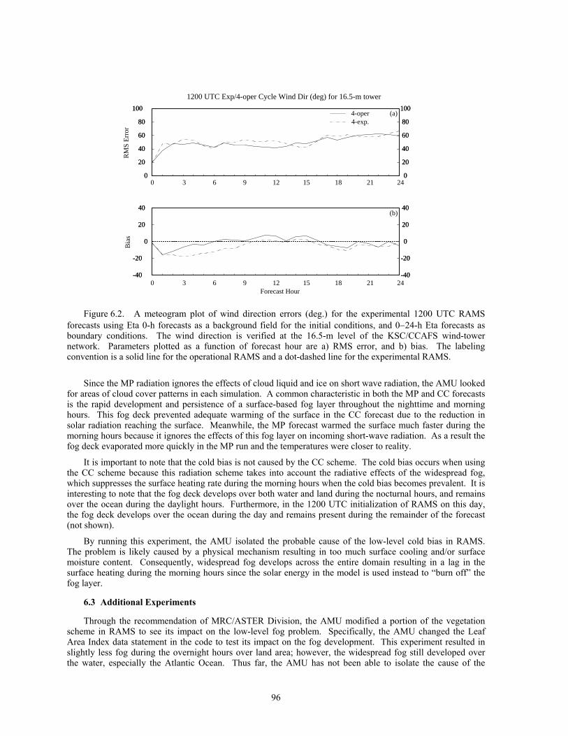
96

0

20

40

60

80

100

0

20

40

60

80

100

10/00 10/02 10/04 10/06 10/08 10/10 10/12 10/14 10/16 10/18 10/20 10/22 11/00-40

-20

0

20

40

-40

-20

0

20

40

0

20

40

60

80

100

0

20

40

60

80

100

10/00 10/02 10/04 10/06 10/08 10/10 10/12 10/14 10/16 10/18 10/20 10/22 11/00-40

-20

0

20

40

-40

-20

0

20

40

(a)

(b)

RM

S E

rror

Bia

s

0 3 6 9 12 15 18 21 24

0 3 6 9 12 15 18 21 24

Forecast Hour

1200 UTC Exp/4-oper Cycle Wind Dir (deg) for 16.5-m tower

4-oper4-exp.

Figure 6.2. A meteogram plot of wind direction errors (deg.) for the experimental 1200 UTC RAMS

forecasts using Eta 0-h forecasts as a background field for the initial conditions, and 0−24-h Eta forecasts as boundary conditions. The wind direction is verified at the 16.5-m level of the KSC/CCAFS wind-tower network. Parameters plotted as a function of forecast hour are a) RMS error, and b) bias. The labeling convention is a solid line for the operational RAMS and a dot-dashed line for the experimental RAMS.

Since the MP radiation ignores the effects of cloud liquid and ice on short wave radiation, the AMU looked for areas of cloud cover patterns in each simulation. A common characteristic in both the MP and CC forecasts is the rapid development and persistence of a surface-based fog layer throughout the nighttime and morning hours. This fog deck prevented adequate warming of the surface in the CC forecast due to the reduction in solar radiation reaching the surface. Meanwhile, the MP forecast warmed the surface much faster during the morning hours because it ignores the effects of this fog layer on incoming short-wave radiation. As a result the fog deck evaporated more quickly in the MP run and the temperatures were closer to reality.

It is important to note that the cold bias is not caused by the CC scheme. The cold bias occurs when using the CC scheme because this radiation scheme takes into account the radiative effects of the widespread fog, which suppresses the surface heating rate during the morning hours when the cold bias becomes prevalent. It is interesting to note that the fog deck develops over both water and land during the nocturnal hours, and remains over the ocean during the daylight hours. Furthermore, in the 1200 UTC initialization of RAMS on this day, the fog deck develops over the ocean during the day and remains present during the remainder of the forecast (not shown).

By running this experiment, the AMU isolated the probable cause of the low-level cold bias in RAMS. The problem is likely caused by a physical mechanism resulting in too much surface cooling and/or surface moisture content. Consequently, widespread fog develops across the entire domain resulting in a lag in the surface heating during the morning hours since the solar energy in the model is used instead to “burn off” the fog layer.

6.3 Additional Experiments

Through the recommendation of MRC/ASTER Division, the AMU modified a portion of the vegetation scheme in RAMS to see its impact on the low-level fog problem. Specifically, the AMU changed the Leaf Area Index data statement in the code to test its impact on the fog development. This experiment resulted in slightly less fog during the overnight hours over land area; however, the widespread fog still developed over the water, especially the Atlantic Ocean. Thus far, the AMU has not been able to isolate the cause of the

97

consistent, rapid development of widespread fog in RAMS. It does appear that this fog phenomenon could be the cause of the low-level cold bias over both land and water.

98

7. Recommendations for Improvements

In this section, the AMU offers some recommendations for modifying and improving the existing ERDAS RAMS forecast and display system. In particular, the AMU highly recommends an improved graphics software package for routine analysis and display of RAMS forecasts. Based on the combination of the objective and subjective evaluations, RAMS clearly offers sufficient added value to short-range forecasts in support of the US Space Program.

7.1 Improve Current Graphics Capabilities

7.1.1 Replace Current RAMS Display

According to the AMU’s assessment, the current graphics software within the MARSS system in the Range Weather Operations (RWO) is not a sufficient interface for displaying and analyzing RAMS forecasts in real-time. There are a number of deficiencies and problems with the display software that make it difficult for any user to efficiently access and analyze forecast data. Some of these deficiencies include:

• Frequent and unpredictable hang-ups and crashes when displaying various combinations of forecast variables.

• Occasional very slow updates when selecting new parameters or grids.

• Inadequate control and insufficient contouring and labeling of scalar fields.

• Very difficult to exit the RAMS interface cleanly without having to kill the existing session.

Other problems may exist with the interface, but these difficulties alone make it quite difficult to use in an operational setting when fast and reliable graphical products are critical.

One alternative to the current RAMS display software that the AMU recommends is the Visualization in 5 dimensions (Vis5D) software. The five dimensions of Vis5D consist of the three spatial dimensions, a dimension in time for animation, and a dimension for displaying multiple variables. Several advantages to using Vis5D as a display software are listed below:

• Vis5D is a visually appealing and easy-to-use display software that gives the user extensive control.

• Vis5D can display horizontal or vertical slices, “isosurfaces” of a constant value in three-dimensions, overlay multiple variables, and can animate all combinations of displays in three-dimensional space.

• A routine already exists within the ERDAS RAMS package to convert the RAMS forecast data into Vis5D format.

• The software is freely available from the University of Wisconsin and can be easily installed onto the existing workstations in the RWO.

• Vis5D has a shallow learning curve and is easy to use the very first time, so required training would be minimal.

Another alternative graphical package is the General Meteorological Package (GEMPAK) software. Available from the Unidata division of the University Corporation for Atmospheric Research, GEMPAK has an extensive amount of capabilities for displaying and computing derived meteorological quantities from gridded forecast fields. As a diagnostic tool, GEMPAK may be more powerful than Vis5D; however, the learning curve for GEMPAK is steeper than Vis5D. Also, in a time-restricted environment, Vis5D would likely provide a snapshot of the forecast data in a shorter time period.

7.1.2 Utilize Real-time Verification Graphical Tool

In addition to utilizing a better graphical software, the AMU also recommends that forecasters use the real-time verification Graphical User Interface (GUI) that is currently available in the RWO. Developed by the AMU, this software allows forecasters to verify RAMS predictions in real-time at both surface and upper-level observational sites. The software incorporates the point forecast data from the current RAMS simulation and

99

plots both observed and forecasts quantities of all available measured variables at a wide range of point locations, including:

• Surface METAR observations,

• KSC/CCAFS wind towers,

• 50-MHz and 915 MHz profilers, and

• All Florida rawinsondes including XMR.

For single point locations such as surface observations, the GUI will plot traces of observed versus forecast quantities for a selected site and weather variable. For upper-level observations such as the wind profilers, the verification GUI will plot time-height cross sections of forecast versus observed quantities according to the availability of both forecast and observed data. In addition, observed and forecast vertical profiles can be compared at a specific time for upper-level locations. Under the ERDAS RAMS options hours task, the AMU improved this graphical software to be more user-friendly and to include additional verification features. Instructions on how to access this real-time GUI, as well as the current display software for viewing RAMS forecasts are provided in Appendix E.

7.2 Improve Data Assimilation and Forecast Cycling

A modification of the current RAMS configuration that would likely reduce the rate of error growth and overall magnitude of the errors is an appropriate data assimilation system. Currently, the Isentropic Analysis (ISAN) package is used to analyze national and local data sets onto each of the RAMS grids at initialization time. RAMS is subsequently “cold-started” from its initial field and integrated for 24 hours. The “cold start” term essentially describes the process of beginning a model run from an initial gridded field without any nudging or data assimilation techniques to bring observational data into balance with the model equations. As a result, cold-start forecasts typically suffer from a swift adjustment in the three-dimensional grid that quickly smoothes out the effects of observational data. The objective error statistics, especially for wind direction, support this statement. The wind direction RMS errors typically doubled in just 1 hour after the initialization time (see Fig. B5 of Appendix B and Fig. C5 of Appendix C).

In addition to the implementation of a data assimilation system, continuous, high-resolution data need to be ingested into the initial condition for RAMS. Observations such as level II WSR-88D reflectivity and radial velocity data, as well as GOES-8 brightness temperatures should be assimilated into the gridded fields to provide the fine details of winds and cloud cover for the model initialization. The high volume of data that WSR-88D and GOES-8 brightness temperatures can provide are very important for correcting the background wind and moisture fields to a more realistic initial condition. Consequently, the model will respond more effectively to the analyzed data because of the continuous nature of these observational data sources.

The analyzed fields with high-resolution observational data can be cycled with RAMS at high temporal frequencies to preserve and better forecast fine-scale features such as thunderstorm outflow boundaries. Initializing RAMS at more frequent intervals (e.g. every 1−3 h as in the NCEP RUC model) will help to accomplish this preservation of detail. Furthermore, additional techniques such as dual-Doppler and thermodynamic retrievals (Lin et al. 1993; Sun and Crook 1996; Shapiro and Mewes 1999) in combination with four-dimensional data assimilation methods (Hoke and Anthes 1976; Bloom et al. 1996) have the potential to provide extensive added value to local high-resolution numerical weather forecasting. As computing power continues to improve in the future, these complex and advanced retrieval techniques can be implemented operationally in combination with a four-dimensional data assimilation scheme. All these techniques have the potential to dramatically improve the quality and accuracy of high-resolution, short-range NWP forecasts.

7.3 Upgrade RAMS to Latest Version

Based on conversations between the AMU and the ASTER Division of MRC, it appears that upgrading RAMS may be the ultimate solution to correct the low-level cold bias in RAMS over east-central Florida and adjacent coastal waters. According to these discussions, RAMS version 4.3 contains a new radiation scheme that alleviates any problems of insufficient shortwave radiation reaching the ground. In addition, MRC notified the AMU that the operational runs using RAMS version 4.3 have no significant biases, and that MRC has not received any reports of biases from other users as well.

100

RAMS version 4.3 still contains a couple drawbacks, though. First, this version still does not incorporate fully-digital vegetation data; however, the subsequent unreleased version 4.4 should contain this digital vegetation data. Second, RAMS currently has only one cumulus/precipitation parameterization scheme, the modified Kuo scheme (Tremback 1990), for simulations on coarse grid resolutions. The Kuo cumulus scheme is the most appropriate for meso-beta grid-spacing scales of 20−200 km. Meanwhile, the current operational configuration of RAMS at CCAFS runs the Kuo cumulus scheme on grids with 15-km and 5-km horizontal resolutions. At these resolutions, an alternative hybrid cumulus scheme should be utilized rather than the Kuo scheme (Molinari and Dudek 1992). At this time, there is no identifiable date when an additional cumulus/precipitation parameterization scheme will be implemented into RAMS in the near future.

101

8. Summary

This report contains results from an objective and subjective evaluation of the RAMS component of ERDAS for the 1999 warm season (May to August), the 1999-2000 cool season (November to March), and the 2000 warm season (May to September) in Florida. The motivation behind this study is to provide an understanding of the model performance and representative errors in the upgraded version of the RAMS in the ERDAS replacement system for both the 45 WS and 45 SW/SE. Two significant changes occurred in the RAMS portion of the replacement system; a full cloud microphysics scheme was implemented on all forecast grids and the innermost nested grid was modified by expanding the domain and improving the horizontal resolution from 3 km to 1.25 km. The primary goal of this task is to determine the accuracy of RAMS forecasts during all seasons and under various weather regimes, concentrating on wind and temperature forecasts that are required for dispersion predictions.

8.1 Summary of the RAMS 4-grid Configuration

The characteristics of the operational RAMS configuration at CCAFS are as follows:

• RAMS runs in real-time using 4 nested grids with horizontal resolutions of 60, 15, 5, and 1.25 km. The high-resolution, innermost nested grid is centered on KSC/CCAFS.

• The RAMS forecast cycle is initialized daily at 0000 and 1200 UTC.

• The model generates an initial condition using the 12-h Eta model forecast as a background field and analyzing local high-resolution data sets including KSC/CCAFS wind towers and profilers.

• RAMS generates a 24-h forecast that typically takes between 10 and 12 h to complete. RAMS forecasts often do not complete all 24 hours due to extensive convection in the model, especially during the warm season. Occasionally, RAMS forecasts do not run because of missing Eta data.

• RAMS forecast output is available once per hour.

8.2 Summary of Objective Evaluation

The objective evaluation in this report was conducted for the 1999-2000 cool season and 2000 warm season months. The objective evaluation consists of five components:

• Evaluation of the operational RAMS configuration during both seasons.

• Regime classification of 2000 warm season forecasts according to observed surface winds.

• Regime classification of 2000 warm season forecasts according to observed versus forecast thunderstorm days.

• Comparison of the operational 4-grid RAMS configuration to a 3-grid configuration for the 1999-2000 cool and 2000 warm seasons, where the innermost grid 4 is withheld during 3-grid forecasts.

• Benchmark of RAMS versus the Eta model for surface predictions at TTS during the 1999-2000 cool and 2000 warm seasons.

Each of these components of the objective evaluation involved the computation of point error statistics (RMS error, bias, and error standard deviation) at all available observational sensors on grid 4, and selected sensors on grids 1, 2, and 3. Among the available observational sensors, the KSC/CCAFS wind-tower network provided the most extensive source of surface verification data on grid 4, and the XMR rawinsonde and 50-MHz DRWP provided the most extensive upper-level verification data on grid 4. However, the 50-MHz DRWP data during the 1999-2000 cool season experienced frequent outages and quality problems. Other sensors used for verification in this report include surface METAR stations and the two buoys offshore of east-central Florida.

102

8.2.1 Operational RAMS Results

RAMS exhibited the following surface and upper-level errors on grid 4 during the 1999-2000 cool and 2000 warm seasons:

Temperature

• Daytime surface and low-level cold bias during both seasons, peaking at -4°C to -4.5°C in the cool season and -2.5°C to -3.5°C in the warm season.

• Cold bias at the buoys at all hours during both seasons, again largest in the cool season (-3°C to -4°C).

• Temperature profile too stable in the troposphere during both seasons.

• The lowest 50 mb or so of the atmosphere are not stable enough in the early morning sounding during both seasons.

• Results are consistent with the 1999 warm-season evaluation in the ERDAS RAMS interim report.

Moisture

• Nocturnal surface moist bias in the cool season of 1−2.5°C.

• Daytime surface dry bias in warm season of -1°C to -2°C.

• Largest dew point temperature errors in mid-levels (5−8°C in the 600−850-mb layer) during both seasons.

Wind Direction

• Rapid growth in surface wind direction errors from 20−40° in the first 2 hours of integration during both seasons.

• Largest errors of about 60−70° occur at the surface during the late night and early morning hours, both seasons.

• Wind direction errors decrease with height, most notably in the cool season where RMS errors are only 10−20° above 500 mb.

• Low-level easterly bias over land, both seasons (u-wind bias of -1 to -2 m s-1, especially during the day in the warm season).

• Southerly bias at all levels above the surface during both seasons.

Wind Speed

• Speed errors increase with height from 2.5 m s-1 near the surface to 5−7 m s-1 at upper-levels, especially in the cool season.

• Positive bias near the surface in both seasons; negative speed bias above 950 mb in the cool season, and above 850 mb in the warm season. The magnitude of all speed biases are generally less than 2 m s-1.

103

8.2.2 Regime Classification Results during the 2000 Warm Season

Surface Wind Classification

• The light wind regime experienced the largest daytime temperature RMS errors (4.5°C) and cold bias (-3.5°C). The wind direction errors were by far the largest during the late night and early morning hours (~ 80−120°) associated with this surface wind regime.

• The westerly wind regime contained the largest random temperature errors (3.5°C), wind direction RMS errors (75°), and u-wind component RMS errors (4.2 m s-1) during the afternoon and evening hours. These errors are likely caused by the presence of the ECSB within the wind tower network during these hours and the high occurrence of convection under surface westerly wind flow.

• The easterly wind regime exhibited the smallest wind direction RMS errors during the daytime (20−30°).

Thunderstorm Day Classification

• The largest daytime random temperature errors (3°C) and wind direction RMS errors (~60°) occurred on days with observed thunderstorms.

• Errors were most dependent on the occurrence of observed thunderstorms and were not that dependent on whether RAMS correctly predicted the thunderstorm day.

8.2.3 4-grid/3-grid RAMS Configuration Comparison

1999-2000 Cool Season

• During the 1999-2000 cool season, the RAMS forecast errors were quite similar for all variables and at all atmospheric levels.

• Temperature errors were slightly larger in the 3-grid configuration at the surface and low-levels whereas the 4-grid configuration contained a greater nocturnal moist bias at the surface.

2000 Warm Season

• The 2000 RAMS warm-season forecast errors exhibited much larger differences than the 1999-2000 cool season, especially in the surface and low-level temperature and dew point temperature forecasts.

• The 3-grid forecasts had much larger surface temperature and dew point temperature RMS errors and a more pronounced cold, dry bias. The dry bias continued during the nocturnal hours of the 3-grid forecasts, but not in the operational 4-grid forecasts.

• Based on these objective results, the higher-resolution configuration of RAMS offers the most improvement during the warm season only.

8.2.4 RAMS/Eta Surface Comparison at TTS

1999-2000 Cool Season

• RAMS had a 3°C daytime cold bias at TTS whereas the Eta model had a 1−2°C warm bias, and since the random errors were comparable, the RMS errors were smallest in the Eta model.

• Both models exhibited a moist bias, which was larger in the Eta model (maximum of 3°C, but only 2°C in RAMS).

104

• The Eta model had slightly smaller wind direction errors by 5−15° at most forecast hours.

2000 Warm Season

• The RAMS cold bias was of the same magnitude as the Eta model’s warm bias and as a result, the total temperature errors were approximately the same.

• The Eta model had a larger moist bias.

• The Eta model exhibited a larger southeasterly bias in winds compared to RAMS, but the overall wind direction errors were smaller in the Eta model.

8.3 Summary of 1999-2000 Cool-Season Subjective Evaluation

The AMU performed a frontal, precipitation, and low-level temperature inversion verification as part of the 1999-2000 cool-season subjective evaluation. For cold frontal verification, the AMU identified observed fronts using GOES-8 infrared imagery and surface stations plots. The AMU subsequently verified RAMS forecast pre-frontal conditions, the changes in temperature, dew point temperature, and wind direction associated with the frontal passage, and the maximum post-frontal wind speed at seven stations along the east coast of the Florida peninsula. During the 1999-2000 cool season, only a few significant precipitation events occurred across the Florida peninsula, so the AMU qualitatively examined each event and summarized the results in a table. The low-level temperature inversion verification was performed for forecasts at the XMR rawinsonde. Observed and forecast temperature inversions were identified and verified in the lowest 3 km of the atmosphere. The results are summarized below.

8.3.1 Frontal Verification

• RAMS pre-frontal temperatures were too cold by 1.6° due to the prevailing low-level cold bias.

• RAMS forecast fronts were generally too weak, given the fact that the average 3-h temperature and dew point temperature decreases associated with the frontal passages were 1.9°C and 4.6°C too small, respectively.

• Forecast post-frontal maximum wind speeds were typically too weak by 2.5 m s-1.

8.3.2 Precipitation Verification

• RAMS demonstrated varying skill in predicting cool-season precipitation patterns.

• The model often missed significant pre-frontal rain bands.

• The problems in adequately predicting frontal-associated precipitation could be caused by large-scale timing errors associated with the Eta model boundary conditions.

8.3.3 Low-level Temperature Inversion Verification

• RAMS predicted only about half of all low-level temperature inversions.

• When successful, RAMS had a tendency to underestimate the magnitude of the temperature inversion (-2.5°C bias).

• Many predicted inversions were not based at the surface, as observed.

8.4 Summary of Subjective Evaluation during the 1999 and 2000 Warm Seasons

The AMU also performed 3 separate verifications in the warm-season subjective evaluation. These three components include a sea-breeze, precipitation, and thunderstorm initiation verification. The sea-breeze verification was composed of three segments:

105

• Verification of operational RAMS sea-breeze forecasts at 12 selected KSC/CCAFS wind towers for May−August 1999 and May−September 2000.

• Comparison of operational 4-grid RAMS to 3-grid RAMS sea-breeze forecasts at the same 12 KSC/CCAFS wind towers during the 2000 warm season only.

• Benchmark of the operational RAMS to the Eta model sea-breeze forecasts at TTS for the 1999 and 2000 warm season.

For the instantaneous precipitation and thunderstorm initiation verifications, RAMS grid 4 was divided into 6 zones, 3 inland and 3 coastal. In the precipitation verification, hourly forecast rain rates of 5 mm h-1 or greater were verified against WSR-74C reflectivities of 32 dBZ or higher. The precipitation verification was conducted during the hours of 1500−2300 UTC every day from June−September 2000.

The thunderstorm initiation verification was also performed daily from 1500−2300 UTC, but for all 2000 warm season months (May−September). The first and subsequent observed thunderstorms were identified according to CGLSS cloud-ground lightning strikes and GOES-8 visible imagery. Meanwhile, the first and subsequent RAMS forecast thunderstorms were identified in zones where predicted vertical velocities at ~7 km exceeded 2 m s-1 in combination with rain rates exceeding 5 mm h-1. The results of each of these subjective verifications are summarized below.

8.4.1 Sea-breeze Verification

Operational RAMS during the 1999 and 2000 Warm Seasons

• RAMS is an excellent predictor of the occurrence of the ECSB within the KSC/CCAFS wind-tower network.

• The 1200 UTC forecast cycle outperformed the 0000 UTC cycle, but both forecast cycles exhibited significant skill (0.56 HSS in 0000 UTC, 0.69 HSS in 1200 UTC forecasts).

• The timing RMS errors associated with the forecast onset of the ECSB are between 1.5 and 2.1 hours at the 12 selected KSC/CCAFS wind towers and only a negligible timing bias occurred.

4-grid/3-grid RAMS Configuration Comparison

• The 4-grid RAMS configuration was significantly better than the 3-grid configuration for both the 0000 and 1200 UTC forecast cycles.

• The most notable improvement occurred in the mainland KSC/CCAFS wind towers, suggesting that the resolution improvement of the 4-grid configuration has a better handle of the sea and river breeze interactions.

• These results also indicate the importance of phenomenological verification in addition to objective error statistics to determine a fine-scale model’s overall potential utility. The objective error statistics do not provide much discernment between the 4-grid and 3-grid RAMS configurations; however, the comparison of the sea-breeze verifications clearly indicates the improvement in ECSB forecasts using the higher-resolution, operational configuration of RAMS.

RAMS/Eta model Comparison

• The RAMS model was statistically more skillful than the Eta model ECSB forecasts at TTS for the 0000 UTC cycle only. Even though the POD was significantly higher in RAMS for the 1200 UTC cycle, so was the bias and FAR. As a result, the 1200 UTC RAMS skill scores were not significantly higher than the Eta model.

• The comparison had limitations in measuring the true skill of RAMS versus the Eta model because no spatial verification of the Eta model at KSC/CCAFS wind towers was conducted.

106

• Based on the combination of objective and subjective comparisons of the RAMS to the Eta model, it appears that the Eta model predicts surface temperatures more accurately than RAMS; however, the RAMS sea-breeze forecasts from the 1.25-km resolution grid demonstrate greater skill in predicting the daily occurrence of the ECSB at TTS.

8.4.2 Precipitation Verification

The precipitation verification results indicated the following about the operational RAMS forecasts:

• The best precipitation forecasts occurred in the inland zones of grid 4 where the POD was about 0.10−0.20 higher than the coastal zones.

• The worst predictions for both forecast cycles occurred in zone 6 (the southeastern part of grid 4) where the POD was generally under 0.30.

• The 1200 UTC cycle generally predicted precipitation better than the 0000 UTC cycle.

• In the 1200 UTC cycle, the most accurate precipitation forecasts occurred during the hours of 1600−2000 UTC when CSI scores (e.g. threat scores) were between 0.25 and 0.40. After 2000 UTC, the CSI scores decreased rapidly to well under 0.20, possibly caused by the model’s inability to adequately forecast the evolution of observed convective outflow boundaries.

8.4.3 Thunderstorm Initiation Verification

The results of the thunderstorm initiation verification yielded the following conclusions:

• The 1200 UTC forecast cycle was a much better predictor of daily thunderstorm occurrence than the 0000 UTC cycle. This result is expected based on the newer initial condition of the 1200 UTC forecast cycle compared to the typical thunderstorm initiation time.

• The 0000 UTC forecast cycle underforecast the occurrence of thunderstorms in all grid-4 zones.

• Thunderstorm occurrence in zone 6 (southeastern part of grid 4) was underforecast by both cycles.

• About 50% of all RAMS forecasts correctly identified one or more zones for daily thunderstorm initiation.

• About 75% of RAMS forecasts identified the timing of thunderstorm initiation to the nearest 3 hours (± 3 h).

The results of the precipitation and thunderstorm initiation verification both could improve by:

• Expanding the lateral boundaries of grid 4 to displace errors resulting from boundary interactions further from the areas of interest.

• Replacing the modified Kuo cumulus parameterization scheme with a hybrid cumulus scheme that is more appropriate for the resolutions used on RAMS grids 2 and 3 (15 km and 5 km).

• Initializing the model soil moisture with actual soil moisture observations and/or archived precipitation data.

• Implementing a four dimensional data assimilation scheme that ingests high-resolution, continuous observational data such as WSR-88D reflectivity and radial velocity, and GOES-8 data.

8.5 Summary of Sensitivity Experiments

The AMU performed various sensitivity tests to isolate the possible cause(s) of the RAMS forecast errors, particularly the low-level cold bias. One of these experiments involved running RAMS using Eta 0-h rather than 12-h forecasts as background fields for the initial conditions. In addition, the 0−24-h rather than the 12−36-h forecasts were used as boundary conditions. This experiment resulted in nearly identical forecast errors.

107

An additional experiment altered the short-wave radiation scheme using the Mahrer-Pielke rather than the operational Chen and Cotton scheme. In the Mahrer-Pielke short-wave radiation scheme, the effects of clouds on short-wave radiation are ignored. In this experimental run, the surface cold bias was dramatically reduced. As a result of this experiment, the AMU discovered that RAMS routinely generates a widespread low-level fog deck across all of grid 4. The fog occurs at night over land and at all times over the ocean. The AMU has not identified the cause of this low-level fog problem.

8.6 Summary of Recommendations

The AMU recommends the following improvements to the existing ERDAS RAMS forecast and display system:

• Improve visualization capabilities by installing Vis5D onto the RWO workstations.

• Implement a four-dimensional data assimilation technique that ingests high-resolution continuous observational data such as WSR-88D reflectivity and radial velocity, and GOES-8 brightness temperature data.

• Initialize RAMS more frequently (e.g. every 1−3 hours) and cycle the model with high-resolution analysis products, much like the current NCEP RUC model.

• Utilize the real-time verification GUI software available in the RWO.

108

9. References

Baldwin, M., 2000: Quantitative precipitation forecast verification documentation. [Available on-line from http://sgi62.wwb.noaa.gov:8080/scores/pptmethod.html.].

Benjamin, S. G., J. M. Brown, K. J. Brundage, D. Devenyi, B. E. Schwartz, T. G. Smirnova, T. L. Smith, L. L. Morone, and G. J. DiMego, 1998: The operational RUC-2. Preprints, 16th Conf. on Weather Analysis and Forecasting, Phoenix, AZ, Amer. Meteor. Soc., 249-252.

Bloom, S. C., L. L. Takacs, A. M. DaSilvia, and D. Ledvina, 1996: Data assimilation using incremental analysis updates. Mon. Wea. Rev., 124, 1256-1271.

Bringi, V. N., K. Knupp, A. Detwiler, L. Liu, I. J. Caylor, and R. A. Black, 1997: Evolution of a Florida thunderstorm during the Convection and Precipitation/Electrification Experiment: The case of 9 August 1991. Mon. Wea. Rev., 125, 2131-2160.

Case, J., 2000: Interim report on the evaluation of the Regional Atmospheric Modeling System in the Eastern Range Dispersion Assessment System. NASA Contractor Report CR-2000-208576, Kennedy Space Center, FL, 102 pp. [Available from ENSCO, Inc., 1980 N. Atlantic Ave., Suite 230, Cocoa Beach, FL 32931].

Cetola, J. D., 1997: A climatology of the sea breeze at Cape Canaveral, Florida. M. S. Thesis, Florida State University, Tallahassee, FL, 56 pp.

Chen, S., and W. R. Cotton, 1988: The sensitivity of a simulated extratropical mesoscale convective system to longwave radiation and ice-phase microphysics. J. Atmos. Sci., 45, 3897-3910.

Cotton, W. R., M. A. Stephens, T. Nehrkorn, and G. J. Tripoli, 1982: The Colorado State University three-dimensional cloud/mesoscale model 1982. Part II: An ice phase parameterization. J. de Rech. Atmos., 16, 295-320.

Davies, H. C., 1983: Limitations of some common lateral boundary schemes used in regional NWP models. Mon. Wea. Rev., 111, 1002-1012.

Doswell, C. A., R. Davies-Jones, and D. Keller, 1990: On summary measures of skill in rare event forecasting based on contingency tables. Wea. Forecasting, 5, 576-585.

Evans, R. J., 1996: Final report on the evaluation of the Emergency Response Dose Assessment System (ERDAS). NASA Contractor Report CR-201353, Kennedy Space Center, FL, 184 pp. [Available from ENSCO Inc., 1980 N. Atlantic Ave., Suite 230, Cocoa Beach, FL 32931].

Hamill, T. M., 1999: Hypothesis tests for evaluating numerical precipitation forecasts. Wea. Forecasting, 14, 155-167.

Hoke, J. E., and R. A. Anthes, 1976: The initialization of numerical models by a dynamical initialization technique. Mon. Wea. Rev., 104, 1551-1556.

Hudlow, M., 1979: Mean rainfall patterns for the three phases of GATE. J. Appl. Meteor., 18, 1656-1669.

Lin, Y., P. S. Ray, and K. W. Johnson, 1993: Initialization of a modeled convective storm using Doppler radar-derived fields. Mon. Wea. Rev., 121, 2757-2775.

López, R. E., and R. L. Holle, 1987: Distribution of summertime lightning as a function of low-level wind flow in central Florida. Technical Memorandum, NOAA Environmental Research Labs, Boulder, CO, 43 p.

109

Lyons, W. A., and C. J. Tremback, 1994: Predicting 3-D wind flows at Cape Canaveral Air Force Station using a mesoscale model. Contract No. F04701-91-C-0058, Los Angeles AFB, CA, 592 pp. [Available from United States Air Force, Space and Missile Systems Center, SMC/CLNE, Los Angeles AFB, CA 90245-4683].

Mahrer, Y., and R. A. Pielke, 1977: A numerical study of the airflow over irregular terrain. Beitr. Phys. Atmos., 50, 98-113.

Manobianco, J., J. W. Zack, and G. E. Taylor, 1996: Workstation-based real-time mesoscale modeling designed for weather support to operations at the Kennedy Space Center and Cape Canaveral Air Station. Bull. Amer. Meteor. Soc., 77, 653-672.

Manobianco, J., and P. A. Nutter, 1999: Evaluation of the 29-km Eta Model. Part II: Subjective verification over Florida. Wea. Forecasting, 14, 18-37.

Mellor, G. L., and T. Yamada, 1982: Development of a turbulence closure model for geophysical fluid problems. Rev. Geophys. Space Phys., 20, 851-875.

Merceret, F. J., 1995: The effect of sensor sheltering and averaging techniques on wind measurements at the Shuttle Landing Facility. NASA Technical Memorandum TM-111262, 42 pp. [Available from NASA Center for Aerospace Information, 7121 Standard Dr., Hanover, MD, 21076-1320.]

Mohanty, U. C., A. Kasahara, and R. Errico, 1986: The impact of diabatic heating on the initialization of a global forecast model. J. Meteor. Soc. Japan, 64, 805-817.

Molinari, J., and M. Dudek, 1992: Parameterization of convective precipitation in mesoscale models: A critical review. Mon. Wea. Rev., 120, 326-344.

Murphy, A. H., 1988: Skill scores based on the mean square error and their relationships to the correlation coefficient. Mon. Wea. Rev., 116, 2417-2424.

Nutter, P. A., and J. Manobianco, 1999: Evaluation of the 29-km Eta Model: Part I: Objective verification at three selected stations. Wea. Forecasting, 14, 5-17.

Olson, D. A., N. W. Junker, and B. Korty, 1995: Evaluation of 33 years of quantitative precipitation forecasting at NMC. Wea. Forecasting, 10, 498-511.

Pielke, R. A., W. R. Cotton, R. L. Walko, C. J. Tremback, W. A. Lyons, L. D. Grasso, M. E. Nicholls, M. D. Morgan, D. A. Wesley, T. J. Lee, and J. H. Copeland, 1992: A comprehensive meteorological modeling system RAMS. Meteor. Atmos. Phys., 49, 69-91.

Reap, R. M., 1994: Analysis and prediction of lightning strike distributions associated with synoptic map types over Florida. Mon. Wea. Rev., 122, 1698-1715.

Salvador, R., J. Calbó, and M. Millán, 1999: Horizontal grid size selection and its influence on mesoscale model simulations. J. Appl. Meteor., 38, 1311-1329.

Schaefer, J. T., 1990: The critical success index as an indicator of warning skill. Wea. Forecasting, 5, 570-575.

Shapiro, A., and J. J. Mewes, 1999: New formulations of dual-Doppler wind analysis. J. Atmos. Oceanic Technol., 16, 782-792.

Schumann, R. S., G. E. Taylor, F. J. Merceret, and T. L. Wilfong, 1999: Performance characteristics of the Kennedy Space Center 50-Mhz Doppler Radar Wind Profiler using the median filter/first-guess data reduction algorithm. J. Atmos. Oceanic Technol., 16, 532-549.

110

Snook, J. S., P. A. Stamus, and J. Edwards, 1998: Local-domain analysis and forecast model support for the 1996 Centennial Olympic Games. Wea. Forecasting, 13, 138-150.

Sun, J., and N. A. Crook, 1996: Comparison of thermodynamic retrieval by the adjoint method with the traditional retrieval. Mon. Wea. Rev., 124, 308-324.

Takano, I. and A. Segami, 1993: Assimilation and initialization of a mesoscale model for improved spin-up of precipitation. J. Meteor. Soc. Japan, 71, 377-391.

Tremback, C. J., 1990: Numerical simulation of a mesoscale convective complex: model development and numerical results. Ph.D. Dissertation, Atmos. Sci. Paper No. 465, Department of Atmospheric Science, Colorado State University, Fort Collins, CO 80523, 247 pp.

Tremback, C. J., and R. Kessler, 1985: A surface temperature and moisture parameterization for use in mesoscale numerical models. Preprints, 7th AMS Conf. on Numerical Weather Prediction, June 17-20, Montreal, Quebec, Amer. Meteor. Soc., Boston, MA, 355-358.

Tremback, C. J., I. T. Baker, M. Uliasz, and R. F. A. Hertenstein, 1998: Time domain reflectometry of soil moisture for initialization of prognostic mesoscale models. Contract No. NAS10-12264, Kennedy Space Center, FL, 339 pp. [Available from Mission Research Corporation / *ASTER Division, PO Box 466, Fort Collins, CO 80522-0466].

Turner, D. B., 1986: Comparison of three methods for calculating the standard deviation of the wind direction. J. Climate Appl. Meteor., 25, 703-707.

Warner, T. T., R. A. Peterson, and R. E. Treadon, 1997: A tutorial on lateral boundary conditions as a basic and potentially serious limitation to regional numerical weather prediction. Bull. Amer. Meteor. Soc., 78, 2599-2617.

____, and H-M. Hsu, 2000: Nested-model simulation of moist convection: The impact of coarse-grid parameterized convection on fine-grid resolved convection. Mon. Wea. Rev., 128, 2211-2231.

Wilks, D. S., 1995: Statistical Methods in the Atmospheric Sciences. Academic Press, 467 pp.

Yuter, S. E., and R. A. Houze Jr., 1995a: Three-dimensional kinematic and microphysical evolution of Florida cumulonimbus. Part I: Spatial distribution of updrafts, downdrafts, and precipitation. Mon. Wea. Rev., 123, 1921-1940.

____, and ____, 1995b: Three-dimensional kinematic and microphysical evolution of Florida cumulonimbus. Part II: Frequency distributions of vertical velocity, reflectivity, and differential reflectivity. Mon. Wea. Rev., 123, 1941-1963.

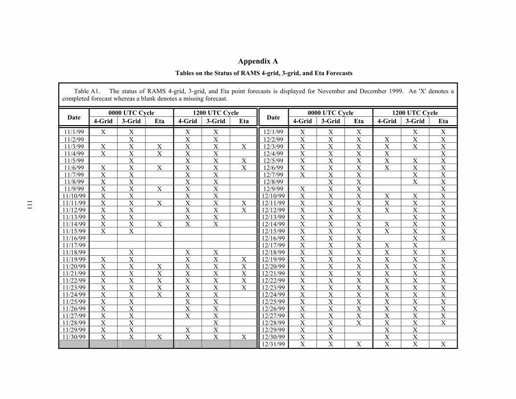
111

Appendix A Tables on the Status of RAMS 4-grid, 3-grid, and Eta Forecasts

Table A1. The status of RAMS 4-grid, 3-grid, and Eta point forecasts is displayed for November and December 1999. An 'X' denotes a completed forecast whereas a blank denotes a missing forecast.

0000 UTC Cycle 1200 UTC Cycle 0000 UTC Cycle 1200 UTC Cycle Date 4-Grid 3-Grid Eta 4-Grid 3-Grid Eta Date 4-Grid 3-Grid Eta 4-Grid 3-Grid Eta

11/1/99 X X X X 12/1/99 X X X X X 11/2/99 X X X 12/2/99 X X X X X X11/3/99 X X X X X X 12/3/99 X X X X X X11/4/99 X X X X X 12/4/99 X X X X X11/5/99 X X X X 12/5/99 X X X X X X11/6/99 X X X X X X 12/6/99 X X X X X X11/7/99 X X X X 12/7/99 X X X X X11/8/99 X X X X 12/8/99 X X X X11/9/99 X X X X X 12/9/99 X X X X

11/10/99 X X X X 12/10/99 X X X X X X11/11/99 X X X X X X 12/11/99 X X X X X X11/12/99 X X X X X 12/12/99 X X X X X X11/13/99 X X X X 12/13/99 X X X X X11/14/99 X X X X X 12/14/99 X X X X X X11/15/99 X X 12/15/99 X X X X X X11/16/99 12/16/99 X X X X X11/17/99 12/17/99 X X X X X11/18/99 X X X 12/18/99 X X X X X X11/19/99 X X X X X 12/19/99 X X X X X X11/20/99 X X X X X X 12/20/99 X X X X X X11/21/99 X X X X X X 12/21/99 X X X X X X11/22/99 X X X X X X 12/22/99 X X X X X X11/23/99 X X X X X X 12/23/99 X X X X X X11/24/99 X X X X X 12/24/99 X X X X X X11/25/99 X X X X 12/25/99 X X X X X X11/26/99 X X X X 12/26/99 X X X X X X11/27/99 X X X X 12/27/99 X X X X X X11/28/99 X X X 12/28/99 X X X X X X11/29/99 X X X X 12/29/99 X X X X11/30/99 X X X X X X 12/30/99 X X X X

12/31/99 X X X X X X

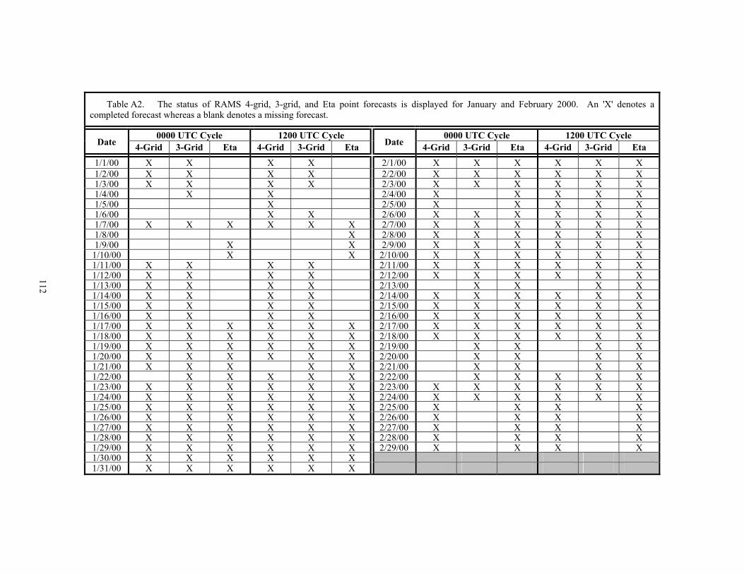
112

Table A2. The status of RAMS 4-grid, 3-grid, and Eta point forecasts is displayed for January and February 2000. An 'X' denotes a completed forecast whereas a blank denotes a missing forecast.

0000 UTC Cycle 1200 UTC Cycle 0000 UTC Cycle 1200 UTC Cycle Date 4-Grid 3-Grid Eta 4-Grid 3-Grid Eta Date 4-Grid 3-Grid Eta 4-Grid 3-Grid Eta

1/1/00 X X X X 2/1/00 X X X X X X 1/2/00 X X X X 2/2/00 X X X X X X1/3/00 X X X X 2/3/00 X X X X X X1/4/00 X X 2/4/00 X X X X X1/5/00 X 2/5/00 X X X X X1/6/00 X X 2/6/00 X X X X X X1/7/00 X X X X X X 2/7/00 X X X X X X1/8/00 X 2/8/00 X X X X X X1/9/00 X X 2/9/00 X X X X X X

1/10/00 X X 2/10/00 X X X X X X1/11/00 X X X X 2/11/00 X X X X X X1/12/00 X X X X 2/12/00 X X X X X X1/13/00 X X X X 2/13/00 X X X X1/14/00 X X X X 2/14/00 X X X X X X1/15/00 X X X X 2/15/00 X X X X X X1/16/00 X X X X 2/16/00 X X X X X X1/17/00 X X X X X X 2/17/00 X X X X X X1/18/00 X X X X X X 2/18/00 X X X X X X1/19/00 X X X X X X 2/19/00 X X X X1/20/00 X X X X X X 2/20/00 X X X X1/21/00 X X X X X 2/21/00 X X X X1/22/00 X X X X X 2/22/00 X X X X X1/23/00 X X X X X X 2/23/00 X X X X X X1/24/00 X X X X X X 2/24/00 X X X X X X1/25/00 X X X X X X 2/25/00 X X X X1/26/00 X X X X X X 2/26/00 X X X X1/27/00 X X X X X X 2/27/00 X X X X1/28/00 X X X X X X 2/28/00 X X X X1/29/00 X X X X X X 2/29/00 X X X X1/30/00 X X X X X X 1/31/00 X X X X X X

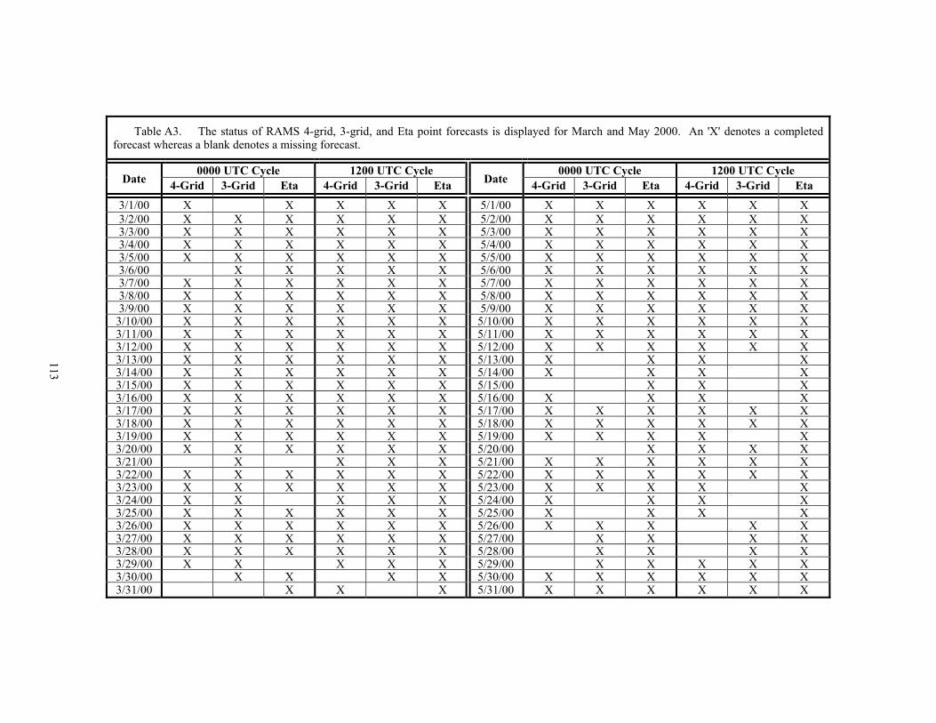
113

Table A3. The status of RAMS 4-grid, 3-grid, and Eta point forecasts is displayed for March and May 2000. An 'X' denotes a completed forecast whereas a blank denotes a missing forecast.

0000 UTC Cycle 1200 UTC Cycle 0000 UTC Cycle 1200 UTC Cycle Date 4-Grid 3-Grid Eta 4-Grid 3-Grid Eta Date 4-Grid 3-Grid Eta 4-Grid 3-Grid Eta

3/1/00 X X X X X 5/1/00 X X X X X X 3/2/00 X X X X X X 5/2/00 X X X X X X3/3/00 X X X X X X 5/3/00 X X X X X X3/4/00 X X X X X X 5/4/00 X X X X X X3/5/00 X X X X X X 5/5/00 X X X X X X3/6/00 X X X X X 5/6/00 X X X X X X3/7/00 X X X X X X 5/7/00 X X X X X X3/8/00 X X X X X X 5/8/00 X X X X X X3/9/00 X X X X X X 5/9/00 X X X X X X

3/10/00 X X X X X X 5/10/00 X X X X X X3/11/00 X X X X X X 5/11/00 X X X X X X3/12/00 X X X X X X 5/12/00 X X X X X X3/13/00 X X X X X X 5/13/00 X X X X3/14/00 X X X X X X 5/14/00 X X X X3/15/00 X X X X X X 5/15/00 X X X3/16/00 X X X X X X 5/16/00 X X X X3/17/00 X X X X X X 5/17/00 X X X X X X3/18/00 X X X X X X 5/18/00 X X X X X X3/19/00 X X X X X X 5/19/00 X X X X X3/20/00 X X X X X X 5/20/00 X X X X3/21/00 X X X X 5/21/00 X X X X X X3/22/00 X X X X X X 5/22/00 X X X X X X3/23/00 X X X X X X 5/23/00 X X X X X3/24/00 X X X X X 5/24/00 X X X X3/25/00 X X X X X X 5/25/00 X X X X3/26/00 X X X X X X 5/26/00 X X X X X3/27/00 X X X X X X 5/27/00 X X X X3/28/00 X X X X X X 5/28/00 X X X X3/29/00 X X X X X 5/29/00 X X X X X3/30/00 X X X X 5/30/00 X X X X X X3/31/00 X X X 5/31/00 X X X X X X

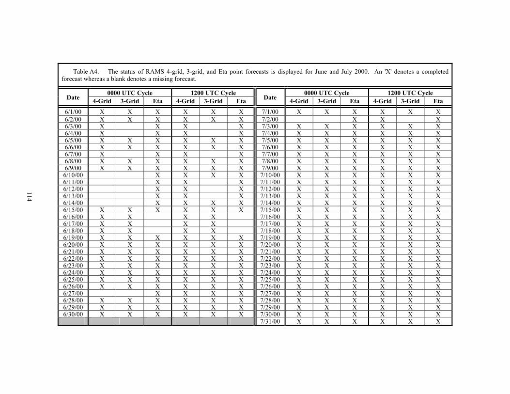
114

Table A4. The status of RAMS 4-grid, 3-grid, and Eta point forecasts is displayed for June and July 2000. An 'X' denotes a completed forecast whereas a blank denotes a missing forecast.

0000 UTC Cycle 1200 UTC Cycle 0000 UTC Cycle 1200 UTC Cycle Date 4-Grid 3-Grid Eta 4-Grid 3-Grid Eta Date 4-Grid 3-Grid Eta 4-Grid 3-Grid Eta

6/1/00 X X X X X X 7/1/00 X X X X X X 6/2/00 X X X X X X 7/2/00 X X X6/3/00 X X X X 7/3/00 X X X X X X6/4/00 X X X X 7/4/00 X X X X X X6/5/00 X X X X X X 7/5/00 X X X X X X6/6/00 X X X X X X 7/6/00 X X X X X X6/7/00 X X X X 7/7/00 X X X X X X6/8/00 X X X X X X 7/8/00 X X X X X X6/9/00 X X X X X X 7/9/00 X X X X X X

6/10/00 X X X X 7/10/00 X X X X X X6/11/00 X X X 7/11/00 X X X X X X6/12/00 X X X 7/12/00 X X X X X X6/13/00 X X X 7/13/00 X X X X X X6/14/00 X X X X 7/14/00 X X X X X X6/15/00 X X X X X X 7/15/00 X X X X X X6/16/00 X X X X 7/16/00 X X X X X X6/17/00 X X X X 7/17/00 X X X X X X6/18/00 X X X X 7/18/00 X X X X X X6/19/00 X X X X X X 7/19/00 X X X X X X6/20/00 X X X X X X 7/20/00 X X X X X X6/21/00 X X X X X X 7/21/00 X X X X X X6/22/00 X X X X X X 7/22/00 X X X X X X6/23/00 X X X X X X 7/23/00 X X X X X X6/24/00 X X X X X X 7/24/00 X X X X X X6/25/00 X X X X X X 7/25/00 X X X X X X6/26/00 X X X X X X 7/26/00 X X X X X X6/27/00 X X X X 7/27/00 X X X X X X6/28/00 X X X X X X 7/28/00 X X X X X X6/29/00 X X X X X X 7/29/00 X X X X X X6/30/00 X X X X X X 7/30/00 X X X X X X

7/31/00 X X X X X X

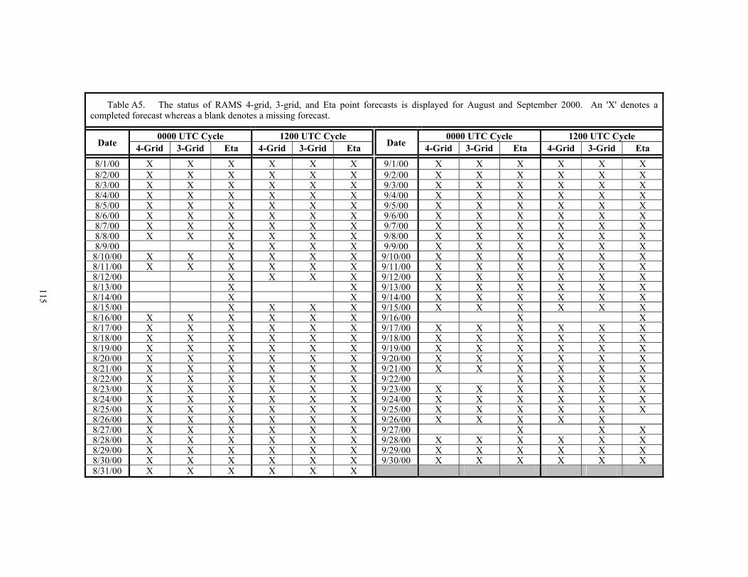
115

Table A5. The status of RAMS 4-grid, 3-grid, and Eta point forecasts is displayed for August and September 2000. An 'X' denotes a completed forecast whereas a blank denotes a missing forecast.

0000 UTC Cycle 1200 UTC Cycle 0000 UTC Cycle 1200 UTC Cycle Date 4-Grid 3-Grid Eta 4-Grid 3-Grid Eta Date 4-Grid 3-Grid Eta 4-Grid 3-Grid Eta

8/1/00 X X X X X X 9/1/00 X X X X X X 8/2/00 X X X X X X 9/2/00 X X X X X X8/3/00 X X X X X X 9/3/00 X X X X X X8/4/00 X X X X X X 9/4/00 X X X X X X8/5/00 X X X X X X 9/5/00 X X X X X X8/6/00 X X X X X X 9/6/00 X X X X X X8/7/00 X X X X X X 9/7/00 X X X X X X8/8/00 X X X X X X 9/8/00 X X X X X X8/9/00 X X X X 9/9/00 X X X X X X

8/10/00 X X X X X X 9/10/00 X X X X X X8/11/00 X X X X X X 9/11/00 X X X X X X8/12/00 X X X X 9/12/00 X X X X X X8/13/00 X X 9/13/00 X X X X X X8/14/00 X X 9/14/00 X X X X X X8/15/00 X X X X 9/15/00 X X X X X X8/16/00 X X X X X X 9/16/00 X X8/17/00 X X X X X X 9/17/00 X X X X X X8/18/00 X X X X X X 9/18/00 X X X X X X8/19/00 X X X X X X 9/19/00 X X X X X X8/20/00 X X X X X X 9/20/00 X X X X X X8/21/00 X X X X X X 9/21/00 X X X X X X8/22/00 X X X X X X 9/22/00 X X X X8/23/00 X X X X X X 9/23/00 X X X X X X8/24/00 X X X X X X 9/24/00 X X X X X X8/25/00 X X X X X X 9/25/00 X X X X X X8/26/00 X X X X X X 9/26/00 X X X X X8/27/00 X X X X X X 9/27/00 X X X8/28/00 X X X X X X 9/28/00 X X X X X X8/29/00 X X X X X X 9/29/00 X X X X X X8/30/00 X X X X X X 9/30/00 X X X X X X8/31/00 X X X X X X

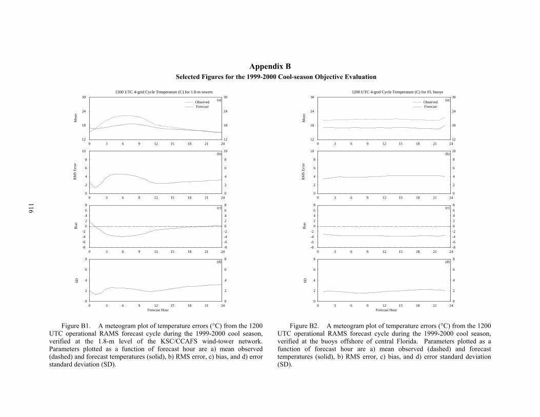
116

Appendix B Selected Figures for the 1999-2000 Cool-season Objective Evaluation

12

18

24

30

12

18

24

30

0

2

4

6

8

10

0

2

4

6

8

10

-8

-6

-4

-2

0

2

4

6

8

-8

-6

-4

-2

0

2

4

6

8

10/00 10/02 10/04 10/06 10/08 10/10 10/12 10/14 10/16 10/18 10/20 10/22 11/000

2

4

6

8

0

2

4

6

8

(a)ObservedForecast

(b)

(c)

(d)

Mea

nR

MS

Err

orB

ias

SD

0 3 6 9 12 15 18 21 24

0 3 6 9 12 15 18 21 24

0 3 6 9 12 15 18 21 24

0 3 6 9 12 15 18 21 24

Forecast Hour

1200 UTC 4-grid Cycle Temperature (C) for 1.8-m towers

Figure B1. A meteogram plot of temperature errors (°C) from the 1200

UTC operational RAMS forecast cycle during the 1999-2000 cool season, verified at the 1.8-m level of the KSC/CCAFS wind-tower network. Parameters plotted as a function of forecast hour are a) mean observed (dashed) and forecast temperatures (solid), b) RMS error, c) bias, and d) error standard deviation (SD).

12

18

24

30

12

18

24

30

0

2

4

6

8

10

0

2

4

6

8

10

-8

-6

-4

-2

0

2

4

6

8

-8

-6

-4

-2

0

2

4

6

8

10/00 10/02 10/04 10/06 10/08 10/10 10/12 10/14 10/16 10/18 10/20 10/22 11/000

2

4

6

8

0

2

4

6

8

(a)ObservedForecast

(b)

(c)

(d)

Mea

nR

MS

Err

orB

ias

SD0 3 6 9 12 15 18 21 24

0 3 6 9 12 15 18 21 24

0 3 6 9 12 15 18 21 24

0 3 6 9 12 15 18 21 24

Forecast Hour

1200 UTC 4-grid Cycle Temperature (C) for FL buoys

Figure B2. A meteogram plot of temperature errors (°C) from the 1200

UTC operational RAMS forecast cycle during the 1999-2000 cool season, verified at the buoys offshore of central Florida. Parameters plotted as a function of forecast hour are a) mean observed (dashed) and forecast temperatures (solid), b) RMS error, c) bias, and d) error standard deviation (SD).

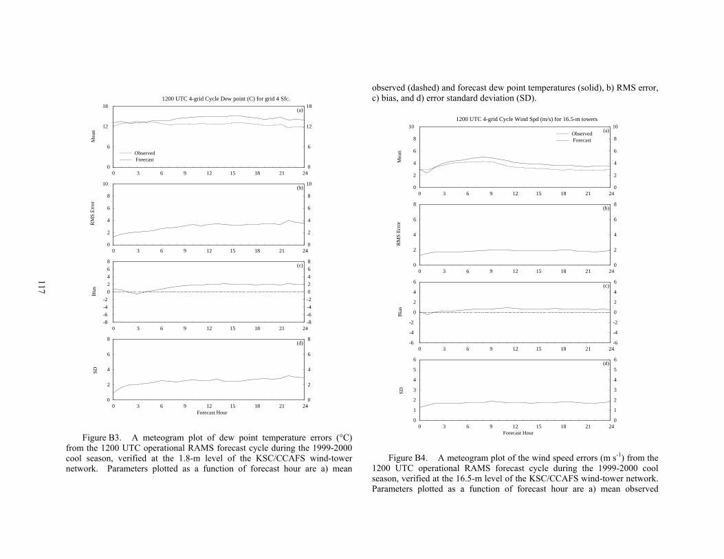
117

0

6

12

18

0

6

12

18

0

2

4

6

8

10

0

2

4

6

8

10

-8

-6

-4

-2

0

2

4

6

8

-8

-6

-4

-2

0

2

4

6

8

10/00 10/02 10/04 10/06 10/08 10/10 10/12 10/14 10/16 10/18 10/20 10/22 11/000

2

4

6

8

0

2

4

6

8

(a)

ObservedForecast

(b)

(c)

(d)

Mea

nR

MS

Err

orB

ias

SD

0 3 6 9 12 15 18 21 24

0 3 6 9 12 15 18 21 24

0 3 6 9 12 15 18 21 24

0 3 6 9 12 15 18 21 24

Forecast Hour

1200 UTC 4-grid Cycle Dew point (C) for grid 4 Sfc.

Figure B3. A meteogram plot of dew point temperature errors (°C)

from the 1200 UTC operational RAMS forecast cycle during the 1999-2000 cool season, verified at the 1.8-m level of the KSC/CCAFS wind-tower network. Parameters plotted as a function of forecast hour are a) mean

observed (dashed) and forecast dew point temperatures (solid), b) RMS error, c) bias, and d) error standard deviation (SD).

0

2

4

6

8

10

0

2

4

6

8

10

0

2

4

6

8

0

2

4

6

8

-6

-4

-2

0

2

4

6

-6

-4

-2

0

2

4

6

10/00 10/02 10/04 10/06 10/08 10/10 10/12 10/14 10/16 10/18 10/20 10/22 11/000

1

2

3

4

5

6

0

1

2

3

4

5

6

(a)ObservedForecast

(b)

(c)

(d)

Mea

nR

MS

Err

orB

ias

SD

0 3 6 9 12 15 18 21 24

0 3 6 9 12 15 18 21 24

0 3 6 9 12 15 18 21 24

0 3 6 9 12 15 18 21 24

Forecast Hour

1200 UTC 4-grid Cycle Wind Spd (m/s) for 16.5-m towers

Figure B4. A meteogram plot of the wind speed errors (m s-1) from the

1200 UTC operational RAMS forecast cycle during the 1999-2000 cool season, verified at the 16.5-m level of the KSC/CCAFS wind-tower network. Parameters plotted as a function of forecast hour are a) mean observed

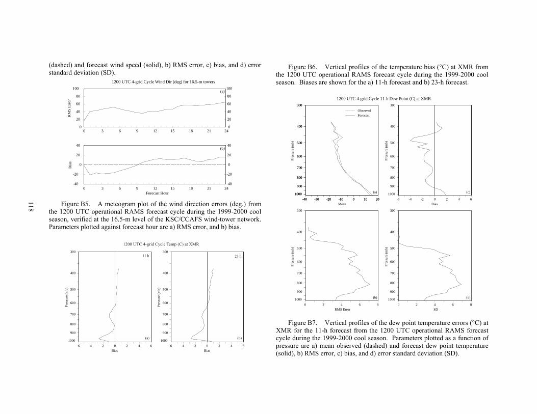
118

(dashed) and forecast wind speed (solid), b) RMS error, c) bias, and d) error standard deviation (SD).

0

20

40

60

80

100

0

20

40

60

80

100

10/00 10/02 10/04 10/06 10/08 10/10 10/12 10/14 10/16 10/18 10/20 10/22 11/00-40

-20

0

20

40

-40

-20

0

20

40

(a)

(b)

RM

S E

rror

Bia

s

0 3 6 9 12 15 18 21 24

0 3 6 9 12 15 18 21 24

Forecast Hour

1200 UTC 4-grid Cycle Wind Dir (deg) for 16.5-m towers

Figure B5. A meteogram plot of the wind direction errors (deg.) from

the 1200 UTC operational RAMS forecast cycle during the 1999-2000 cool season, verified at the 16.5-m level of the KSC/CCAFS wind-tower network. Parameters plotted against forecast hour are a) RMS error, and b) bias.

(a) (b)

1200 UTC 4-grid Cycle Temp (C) at XMR

11 h 23 h

-6 -4 -2 0 2 4 6

300

400

500

600

700

800

900

1000

Bias

Pres

sure

(m

b)

-6 -4 -2 0 2 4 6

300

400

500

600

700

800

900

1000

Bias

Pres

sure

(m

b)

Figure B6. Vertical profiles of the temperature bias (°C) at XMR from the 1200 UTC operational RAMS forecast cycle during the 1999-2000 cool season. Biases are shown for the a) 11-h forecast and b) 23-h forecast.

-40 -30 -20 -10 0 10 20

300

400

500

600

700

800

900

1000

-40 -30 -20 -10 0 10 20

300

400

500

600

700

800

900

1000

0 2 4 6 8

300

400

500

600

700

800

900

1000

0 2 4 6 8

300

400

500

600

700

800

900

1000

-6 -4 -2 0 2 4 6

300

400

500

600

700

800

900

1000

ObservedForecast

Mean

(a)

RMS Error

(b)

SD

(d)

Bias

(c)

Pres

sure

(m

b)

Pres

sure

(m

b)

Pres

sure

(m

b)

Pres

sure

(m

b)

1200 UTC 4-grid Cycle 11-h Dew Point (C) at XMR

Figure B7. Vertical profiles of the dew point temperature errors (°C) at

XMR for the 11-h forecast from the 1200 UTC operational RAMS forecast cycle during the 1999-2000 cool season. Parameters plotted as a function of pressure are a) mean observed (dashed) and forecast dew point temperature (solid), b) RMS error, c) bias, and d) error standard deviation (SD).

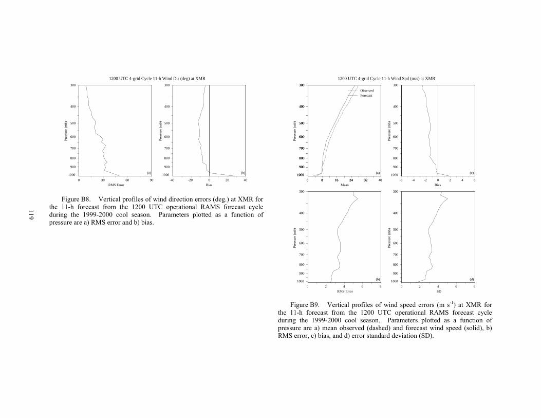
119

0 30 60 90

300

400

500

600

700

800

900

1000

-40 -20 0 20 40

300

400

500

600

700

800

900

1000

RMS Error

(a)

Bias

(b)

Pres

sure

(m

b)

Pres

sure

(m

b)

1200 UTC 4-grid Cycle 11-h Wind Dir (deg) at XMR

Figure B8. Vertical profiles of wind direction errors (deg.) at XMR for

the 11-h forecast from the 1200 UTC operational RAMS forecast cycle during the 1999-2000 cool season. Parameters plotted as a function of pressure are a) RMS error and b) bias.

0 8 16 24 32 40

300

400

500

600

700

800

900

1000

0 8 16 24 32 40

300

400

500

600

700

800

900

1000

0 2 4 6 8

300

400

500

600

700

800

900

1000

0 2 4 6 8

300

400

500

600

700

800

900

1000

-6 -4 -2 0 2 4 6

300

400

500

600

700

800

900

1000

ObservedForecast

Mean

(a)

RMS Error

(b)

SD

(d)

Bias

(c)

Pres

sure

(m

b)

Pres

sure

(m

b)

Pres

sure

(m

b)

Pres

sure

(m

b)

1200 UTC 4-grid Cycle 11-h Wind Spd (m/s) at XMR

Figure B9. Vertical profiles of wind speed errors (m s-1) at XMR for

the 11-h forecast from the 1200 UTC operational RAMS forecast cycle during the 1999-2000 cool season. Parameters plotted as a function of pressure are a) mean observed (dashed) and forecast wind speed (solid), b) RMS error, c) bias, and d) error standard deviation (SD).

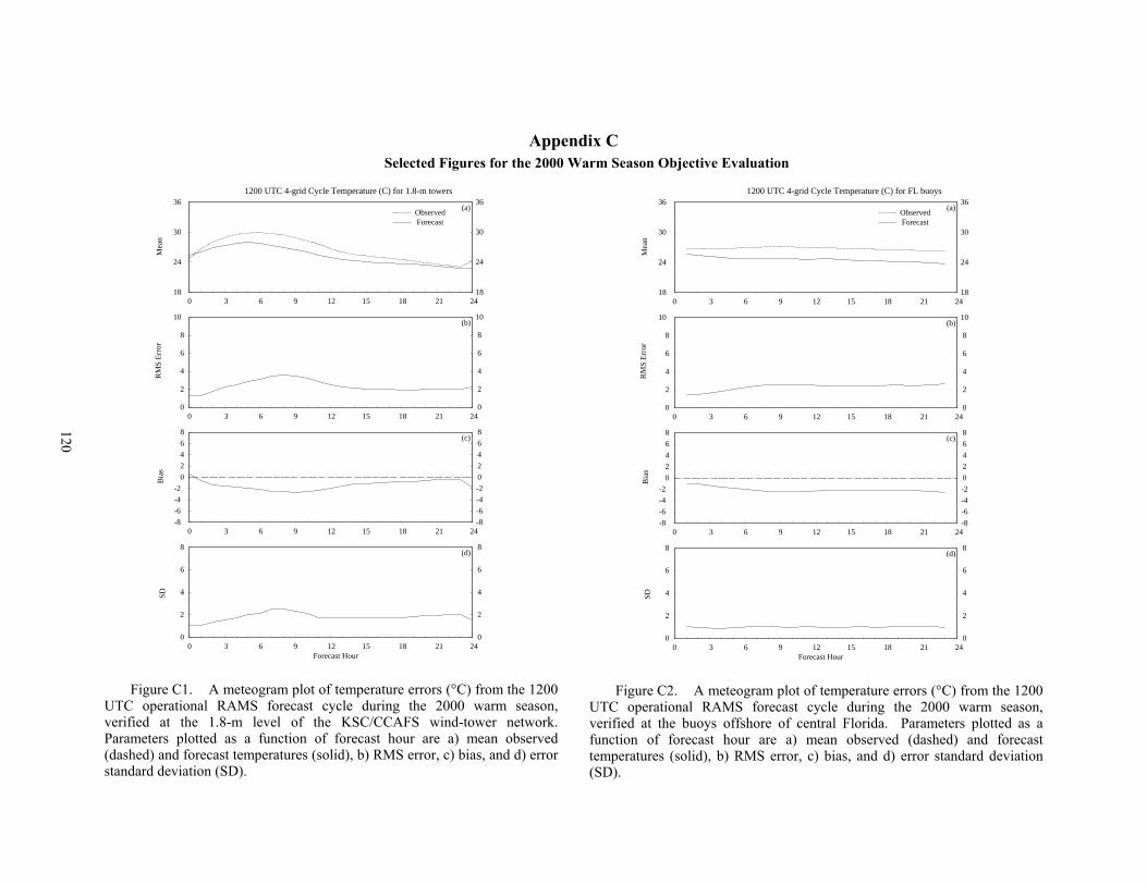
120

Appendix C Selected Figures for the 2000 Warm Season Objective Evaluation

18

24

30

36

18

24

30

36

0

2

4

6

8

10

0

2

4

6

8

10

-8

-6

-4

-2

0

2

4

6

8

-8

-6

-4

-2

0

2

4

6

8

10/00 10/02 10/04 10/06 10/08 10/10 10/12 10/14 10/16 10/18 10/20 10/22 11/000

2

4

6

8

0

2

4

6

8

(a)ObservedForecast

(b)

(c)

(d)

Mea

nR

MS

Err

orB

ias

SD

0 3 6 9 12 15 18 21 24

0 3 6 9 12 15 18 21 24

0 3 6 9 12 15 18 21 24

0 3 6 9 12 15 18 21 24

Forecast Hour

1200 UTC 4-grid Cycle Temperature (C) for 1.8-m towers

Figure C1. A meteogram plot of temperature errors (°C) from the 1200

UTC operational RAMS forecast cycle during the 2000 warm season, verified at the 1.8-m level of the KSC/CCAFS wind-tower network. Parameters plotted as a function of forecast hour are a) mean observed (dashed) and forecast temperatures (solid), b) RMS error, c) bias, and d) error standard deviation (SD).

18

24

30

36

18

24

30

36

0

2

4

6

8

10

0

2

4

6

8

10

-8

-6

-4

-2

0

2

4

6

8

-8

-6

-4

-2

0

2

4

6

8

10/00 10/02 10/04 10/06 10/08 10/10 10/12 10/14 10/16 10/18 10/20 10/22 11/000

2

4

6

8

0

2

4

6

8

(a)ObservedForecast

(b)

(c)

(d)

Mea

nR

MS

Err

orB

ias

SD0 3 6 9 12 15 18 21 24

0 3 6 9 12 15 18 21 24

0 3 6 9 12 15 18 21 24

0 3 6 9 12 15 18 21 24

Forecast Hour

1200 UTC 4-grid Cycle Temperature (C) for FL buoys

Figure C2. A meteogram plot of temperature errors (°C) from the 1200

UTC operational RAMS forecast cycle during the 2000 warm season, verified at the buoys offshore of central Florida. Parameters plotted as a function of forecast hour are a) mean observed (dashed) and forecast temperatures (solid), b) RMS error, c) bias, and d) error standard deviation (SD).

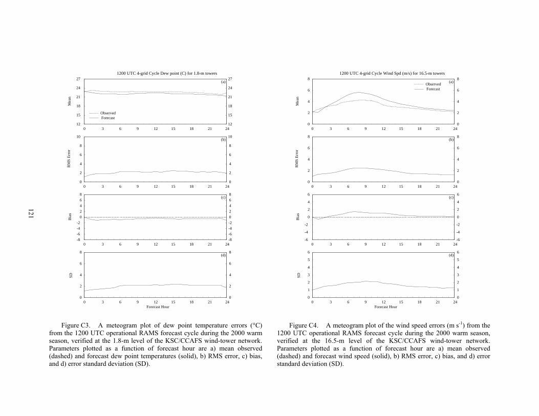
121

12

15

18

21

24

27

12

15

18

21

24

27

0

2

4

6

8

10

0

2

4

6

8

10

-8

-6

-4

-2

0

2

4

6

8

-8

-6

-4

-2

0

2

4

6

8

10/00 10/02 10/04 10/06 10/08 10/10 10/12 10/14 10/16 10/18 10/20 10/22 11/000

2

4

6

8

0

2

4

6

8

(a)

ObservedForecast

(b)

(c)

(d)

Mea

nR

MS

Err

orB

ias

SD

0 3 6 9 12 15 18 21 24

0 3 6 9 12 15 18 21 24

0 3 6 9 12 15 18 21 24

0 3 6 9 12 15 18 21 24

Forecast Hour

1200 UTC 4-grid Cycle Dew point (C) for 1.8-m towers

Figure C3. A meteogram plot of dew point temperature errors (°C)

from the 1200 UTC operational RAMS forecast cycle during the 2000 warm season, verified at the 1.8-m level of the KSC/CCAFS wind-tower network. Parameters plotted as a function of forecast hour are a) mean observed (dashed) and forecast dew point temperatures (solid), b) RMS error, c) bias, and d) error standard deviation (SD).

0

2

4

6

8

0

2

4

6

8

0

2

4

6

8

0

2

4

6

8

-6

-4

-2

0

2

4

6

-6

-4

-2

0

2

4

6

10/00 10/02 10/04 10/06 10/08 10/10 10/12 10/14 10/16 10/18 10/20 10/22 11/000

1

2

3

4

5

6

0

1

2

3

4

5

6

(a)ObservedForecast

(b)

(c)

(d)

Mea

nR

MS

Err

orB

ias

SD0 3 6 9 12 15 18 21 24

0 3 6 9 12 15 18 21 24

0 3 6 9 12 15 18 21 24

0 3 6 9 12 15 18 21 24

Forecast Hour

1200 UTC 4-grid Cycle Wind Spd (m/s) for 16.5-m towers

Figure C4. A meteogram plot of the wind speed errors (m s-1) from the

1200 UTC operational RAMS forecast cycle during the 2000 warm season, verified at the 16.5-m level of the KSC/CCAFS wind-tower network. Parameters plotted as a function of forecast hour are a) mean observed (dashed) and forecast wind speed (solid), b) RMS error, c) bias, and d) error standard deviation (SD).

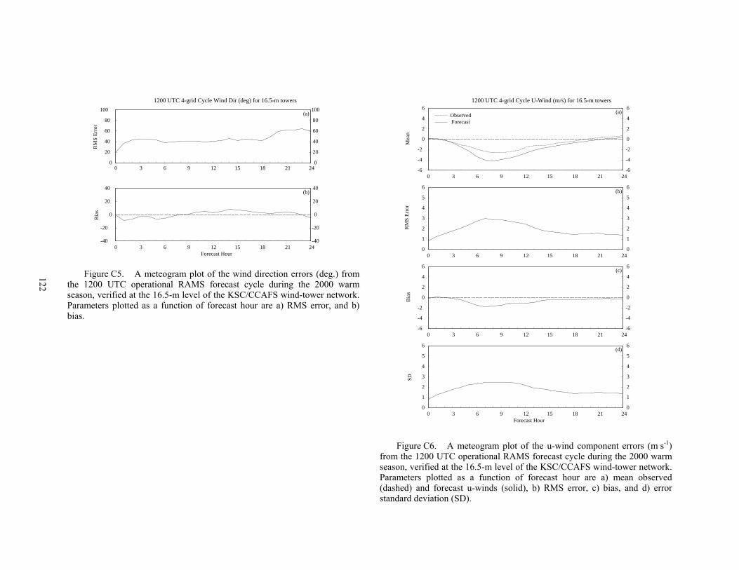
122

0

20

40

60

80

100

0

20

40

60

80

100

10/00 10/02 10/04 10/06 10/08 10/10 10/12 10/14 10/16 10/18 10/20 10/22 11/00-40

-20

0

20

40

-40

-20

0

20

40

(a)

(b)

RM

S E

rror

Bia

s

0 3 6 9 12 15 18 21 24

0 3 6 9 12 15 18 21 24

Forecast Hour

1200 UTC 4-grid Cycle Wind Dir (deg) for 16.5-m towers

Figure C5. A meteogram plot of the wind direction errors (deg.) from

the 1200 UTC operational RAMS forecast cycle during the 2000 warm season, verified at the 16.5-m level of the KSC/CCAFS wind-tower network. Parameters plotted as a function of forecast hour are a) RMS error, and b) bias.

-6

-4

-2

0

2

4

6

-6

-4

-2

0

2

4

6

0

1

2

3

4

5

6

0

1

2

3

4

5

6

-6

-4

-2

0

2

4

6

-6

-4

-2

0

2

4

6

10/00 10/02 10/04 10/06 10/08 10/10 10/12 10/14 10/16 10/18 10/20 10/22 11/000

1

2

3

4

5

6

0

1

2

3

4

5

6

(a)ObservedForecast

(b)

(c)

(d)

Mea

nR

MS

Err

orB

ias

SD0 3 6 9 12 15 18 21 24

0 3 6 9 12 15 18 21 24

0 3 6 9 12 15 18 21 24

0 3 6 9 12 15 18 21 24

Forecast Hour

1200 UTC 4-grid Cycle U-Wind (m/s) for 16.5-m towers

Figure C6. A meteogram plot of the u-wind component errors (m s-1)

from the 1200 UTC operational RAMS forecast cycle during the 2000 warm season, verified at the 16.5-m level of the KSC/CCAFS wind-tower network. Parameters plotted as a function of forecast hour are a) mean observed (dashed) and forecast u-winds (solid), b) RMS error, c) bias, and d) error standard deviation (SD).

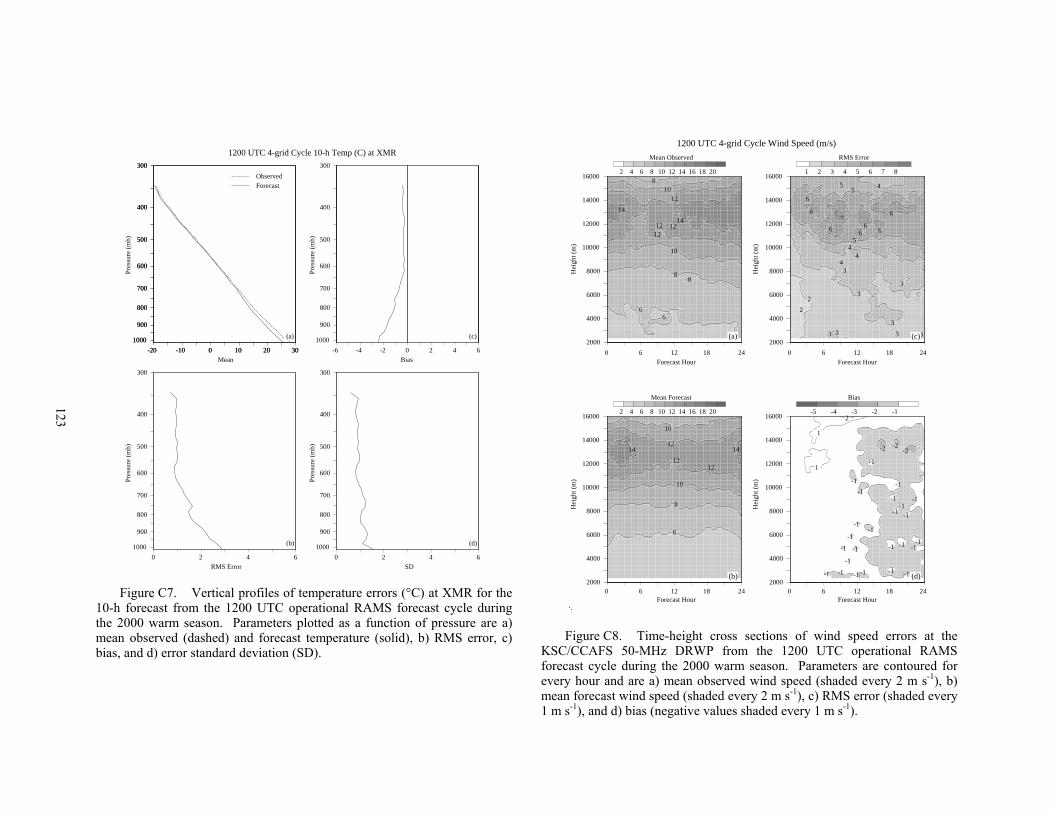
123

-20 -10 0 10 20 30

300

400

500

600

700

800

900

1000

-20 -10 0 10 20 30

300

400

500

600

700

800

900

1000

0 2 4 6

300

400

500

600

700

800

900

1000

0 2 4 6

300

400

500

600

700

800

900

1000

-6 -4 -2 0 2 4 6

300

400

500

600

700

800

900

1000

ObservedForecast

Mean

(a)

RMS Error

(b)

SD

(d)

Bias

(c)

Pres

sure

(m

b)

Pres

sure

(m

b)

Pres

sure

(m

b)

Pres

sure

(m

b)

1200 UTC 4-grid Cycle 10-h Temp (C) at XMR

Figure C7. Vertical profiles of temperature errors (°C) at XMR for the

10-h forecast from the 1200 UTC operational RAMS forecast cycle during the 2000 warm season. Parameters plotted as a function of pressure are a) mean observed (dashed) and forecast temperature (solid), b) RMS error, c) bias, and d) error standard deviation (SD).

66

8

88

10

10

12

1212 12

14

14

2000

4000

6000

8000

10000

12000

14000

160002 4 6 8 10 12 14 16 18 20

Mean Observed

6

8

10

10

12

1212

1414

2000

4000

6000

8000

10000

12000

14000

160002 4 6 8 10 12 14 16 18 20

Mean Forecast

2

2

3

3

3

3

3

33 3

4

44

4

5

5

5

6

6

6

6

666

7

2000

4000

6000

8000

10000

12000

14000

160001 2 3 4 5 6 7 8

RMS Error

-2 -2-2

-1

-1

-1

-1

-1

-1-1

-1-1

-1-1

-1-1

-1-1 -1-1 -1

-1

-1-1-1 -1-1 -1

1

1

2

2000

4000

6000

8000

10000

12000

14000

16000-5 -4 -3 -2 -1

Bias

(a)

0 6 12 18 24Forecast Hour

Hei

ght (

m)

1200 UTC 4-grid Cycle Wind Speed (m/s)

(c)

0 6 12 18 24Forecast Hour

Hei

ght (

m)

(b)

0 6 12 18 24Forecast Hour

Hei

ght (

m)

(d)

0 6 12 18 24Forecast Hour

Hei

ght (

m)

Figure C8. Time-height cross sections of wind speed errors at the

KSC/CCAFS 50-MHz DRWP from the 1200 UTC operational RAMS forecast cycle during the 2000 warm season. Parameters are contoured for every hour and are a) mean observed wind speed (shaded every 2 m s-1), b) mean forecast wind speed (shaded every 2 m s-1), c) RMS error (shaded every 1 m s-1), and d) bias (negative values shaded every 1 m s-1).

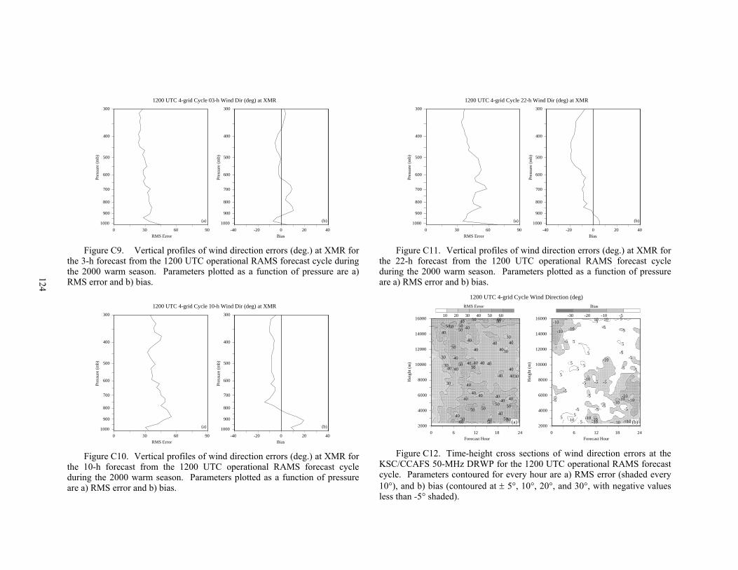
124

0 30 60 90

300

400

500

600

700

800

900

1000

-40 -20 0 20 40

300

400

500

600

700

800

900

1000

RMS Error

(a)

Bias

(b)

Pres

sure

(m

b)

Pres

sure

(m

b)

1200 UTC 4-grid Cycle 03-h Wind Dir (deg) at XMR

Figure C9. Vertical profiles of wind direction errors (deg.) at XMR for

the 3-h forecast from the 1200 UTC operational RAMS forecast cycle during the 2000 warm season. Parameters plotted as a function of pressure are a) RMS error and b) bias.

0 30 60 90

300

400

500

600

700

800

900

1000

-40 -20 0 20 40

300

400

500

600

700

800

900

1000

RMS Error

(a)

Bias

(b)

Pres

sure

(m

b)

Pres

sure

(m

b)

1200 UTC 4-grid Cycle 10-h Wind Dir (deg) at XMR

Figure C10. Vertical profiles of wind direction errors (deg.) at XMR for

the 10-h forecast from the 1200 UTC operational RAMS forecast cycle during the 2000 warm season. Parameters plotted as a function of pressure are a) RMS error and b) bias.

0 30 60 90

300

400

500

600

700

800

900

1000

-40 -20 0 20 40

300

400

500

600

700

800

900

1000

RMS Error

(a)

Bias

(b)

Pres

sure

(m

b)

Pres

sure

(m

b)

1200 UTC 4-grid Cycle 22-h Wind Dir (deg) at XMR

Figure C11. Vertical profiles of wind direction errors (deg.) at XMR for

the 22-h forecast from the 1200 UTC operational RAMS forecast cycle during the 2000 warm season. Parameters plotted as a function of pressure are a) RMS error and b) bias.

30

30

30

3030

3040

40

40

4040

4040

40

40 40

4040 40 40

40 40

40 40

40

4040 4040 4040

40 4040

50 50

50

5050 5050

50

5050

5050

50

50505050

60

602000

4000

6000

8000

10000

12000

14000

1600010 20 30 40 50 60

RMS Error

-10

-10

-10

-10

-10

-10

-10-10

-10

-10 -10 -10-10-10

-5

-5

-5

-5

-5-5

-5

-5 -5

-5 -5

-5-5

-5-5

-5-5

55

5 5

5

5 55

5

55

5

10 10

102000

4000

6000

8000

10000

12000

14000

16000-30 -20 -10 -5

Bias

(a)

0 6 12 18 24Forecast Hour

Hei

ght (

m)

1200 UTC 4-grid Cycle Wind Direction (deg)

(b)

0 6 12 18 24Forecast Hour

Hei

ght (

m)

Figure C12. Time-height cross sections of wind direction errors at the

KSC/CCAFS 50-MHz DRWP for the 1200 UTC operational RAMS forecast cycle. Parameters contoured for every hour are a) RMS error (shaded every 10°), and b) bias (contoured at ± 5°, 10°, 20°, and 30°, with negative values less than -5° shaded).

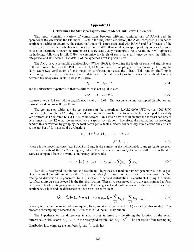
125

Appendix D Determining the Statistical Significance of Model Skill Scores Differences

This report contains a variety of comparisons between different configurations of RAMS and the operational RAMS versus the Eta model. Within the subjective evaluation, the AMU composed a number of contingency tables to determine the categorical and skill scores associated with RAMS and Eta forecasts of the ECSB. In order to claim whether one model is more skillful than another, an appropriate hypothesis test must be used to determine whether the different results are statistically meaningful. As a result, the AMU applied a methodology following Hamill (1999) to determine the levels of statistical significance between the different categorical and skill scores. The details of the hypothesis test is given below.

The AMU used a resampling methodology (Wilks 1995) to determine the levels of statistical significance in the differences between the POD, FAR, CSI, HSS, and bias. Resampling involves randomly shuffling the daily sea-breeze verification of one model or configuration versus the other. This random shuffling is performing many times to obtain a sufficient data base. The null hypothesis for this test is that the differences between the categorical or skill scores (S) is zero:

H0: S1 - S2 = 0.0, (D1)

and the alternative hypothesis is that the difference is not equal to zero:

HA: S1 - S2 ≠ 0.0. (D2)

Assume a two-sided test with a significance level α = 0.05. The test statistic and resampled distribution are formed based on this null hypothesis.

The contingency tables for the comparisons of the operational RAMS 0000 UTC versus 1200 UTC forecast cycles and the RAMS 4-grid/3-grid configurations involved contingency tables developed from daily verifications at 12 selected KSC/CCAFS wind towers. On a given day, it is likely that the forecast sea-breeze occurrences at the 12 wind towers experience a spatial correlation. Therefore, the resampling methodology handles this correlation by grouping the total contingency table elements for each day into a vector array of size n, the number of days during the evaluation:

( ) jiji dcba ,, ,,,=x , i = 1,2, and

j = 1,…, n, (D3)

where i is the model indicator (e.g. RAMS or Eta), j is the number of the individual day, and (a,b,c,d) represent the four elements of the 2 x 2 contingency table. The test statistic is simply the actual difference in the skill score as computed from the overall contingency table results:

( ) ( ) ( ) ∑∑==

−=−=−n

kk

n

kkdcbadcbaSS

1,2

1,12121 ,,,,,,ˆˆ xx . (D4)

To build a resampled distribution and test the null hypothesis, a random number generator is used to pick either one model (configuration) or the other on each day (1,…., n) from the two vector arrays. After the first resampled distribution is generated by this method, a second distribution is constructed using the model (configuration) data not selected in the first distribution. These two resampled arrays are each summed to form two new sets of contingency table elements. The categorical and skill scores are calculated for these two contingency tables and the differences in the scores are computed:

( ) ( ) ( ) ∑∑=

−=

−=−=−n

kkI

n

kkI kk

dcbadcbaSS1

),3(1

,*2

*1

*2

*1 ,,,,,,ˆˆ xx , (D5)

where Ik is a random number indicator equally likely to take on the value 1 or 2 (one or the other model). This process of resampling is repeated 10,000 times to build the null distribution.

The hypothesis of the differences in skill scores is tested by identifying the location of the actual differences in skill scores, ( )21

ˆˆ SS − , in the resampled distribution, ( )*2

*1

ˆˆ SS − . The net result of the resampling

distribution is to compute the numbers Lt̂ and Vt̂ such that

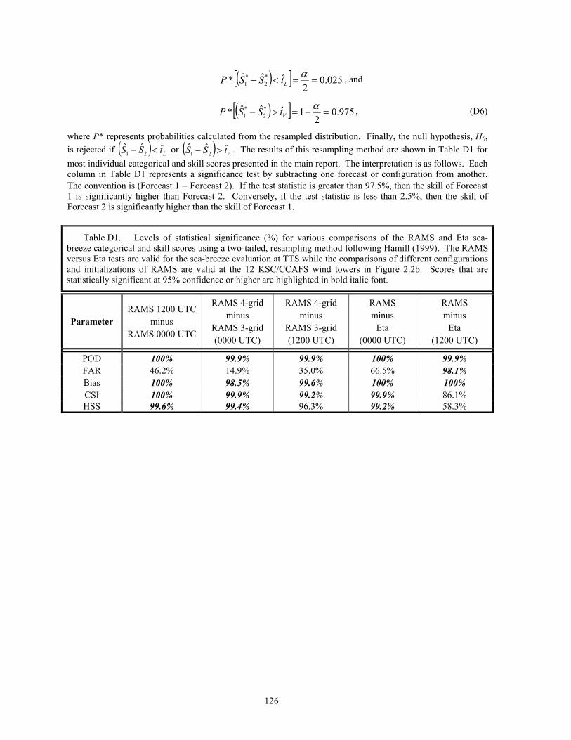
126

( )[ ] 025.02

ˆˆˆ* *2

*1 ==<−

αLtSSP , and

( )[ ] 975.02

1ˆˆˆ* *2

*1 =−=>−

αVtSSP , (D6)

where P* represents probabilities calculated from the resampled distribution. Finally, the null hypothesis, H0, is rejected if ( ) LtSS ˆˆˆ

21 <− or ( ) VtSS ˆˆˆ21 >− . The results of this resampling method are shown in Table D1 for

most individual categorical and skill scores presented in the main report. The interpretation is as follows. Each column in Table D1 represents a significance test by subtracting one forecast or configuration from another. The convention is (Forecast 1 − Forecast 2). If the test statistic is greater than 97.5%, then the skill of Forecast 1 is significantly higher than Forecast 2. Conversely, if the test statistic is less than 2.5%, then the skill of Forecast 2 is significantly higher than the skill of Forecast 1.

Table D1. Levels of statistical significance (%) for various comparisons of the RAMS and Eta sea-breeze categorical and skill scores using a two-tailed, resampling method following Hamill (1999). The RAMS versus Eta tests are valid for the sea-breeze evaluation at TTS while the comparisons of different configurations and initializations of RAMS are valid at the 12 KSC/CCAFS wind towers in Figure 2.2b. Scores that are statistically significant at 95% confidence or higher are highlighted in bold italic font.

Parameter RAMS 1200 UTC

minus RAMS 0000 UTC

RAMS 4-grid minus

RAMS 3-grid (0000 UTC)

RAMS 4-grid minus

RAMS 3-grid (1200 UTC)

RAMS minus

Eta (0000 UTC)

RAMS minus

Eta (1200 UTC)

POD 100% 99.9% 99.9% 100% 99.9% FAR 46.2% 14.9% 35.0% 66.5% 98.1% Bias 100% 98.5% 99.6% 100% 100% CSI 100% 99.9% 99.2% 99.9% 86.1% HSS 99.6% 99.4% 96.3% 99.2% 58.3%

127

Appendix E Quick Guide to Accessing RAMS Forecasts and the Real-time Verification Graphical User Interface

E1. RAMS Graphical User Interface Startup

Beginning with the MARSS window in upper-left of screen (Meteorological and Range Safety Support System), perform the following actions:

• On MARSS windows menu, click on MODELS/ERDAS, and 3 new windows will load:

1. ERDAS Operational Status Window (provides status of current RAMS model run), 2. ERDAS Meteorology (control panel for displaying forecast variables), and 3. ERDAS View (display window).

• To view enhanced graphics: Click on TOOLS/ENHANCED GRAPHICS and two windows will load:

1. RAMS Interactive NCAR Graphics (Control panel), and 2. RingiView (display window).

• The capabilities include looping, zooming, cross sections, and overlay fields.

• To quit enhanced graphics: Click on FILE/QUIT.

• To quit the initial menu: Click on FILE/QUIT ERDAS (Confirmation window will load: click "OK").

(Note: In the event that the ERDAS RAMS GUI freezes or locks up, the current session must be terminated. To kill the current session, simply start up a new ERDAS RAMS window from the MARSS window menu. A new window will ask if you want to kill the current session. Click yes.)

E2. RAMS Real-time Verification Graphical User Interface

Beginning with toolbar at the bottom of the screen, perform the following actions:

• Click on small up arrow above the miniature map icon (bottom of screen),

• Click on rw_profiler,

• Type in the forecast time to verify,

1. Format: yyyy-mo-dd-hhmm 2. yyyy=year, mo=month, dd=day, hh=hour, mm=minute. 3. Example: 1999-12-15-1200 = 1200 UTC RAMS forecast run on 15 December 1999.

• A window will pop up which offers a variety of verification tools, including:

1. Verification at various sensors: 915-MHz (RWP915) and 50-MHz (RWP50) profilers, Florida (NATLRWS) and Cape Canaveral (CAPERWS) rawinsondes, KSC/CCAFS wind towers (TOWER), surface METAR (SFC OBS) stations, and buoys (BUOY). Simply click the tab in the upper left corner below "file" to choose a different observation type.

2. Verification of different parameters: Click on the OPTIONS menu to choose among:

a) Wind barb time series, b) Wind barb by sensor, c) Temperature/dew point temperature graph, d) Wind speed/direction graph, e) Surface winds, and f) Surface temperature and dew point temperature.

3. To exit: Click on FILE/EXIT.

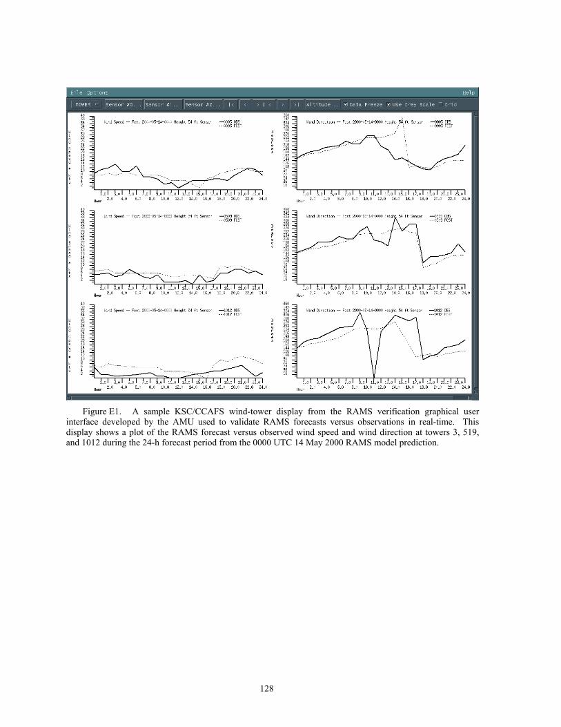
128

Figure E1. A sample KSC/CCAFS wind-tower display from the RAMS verification graphical user

interface developed by the AMU used to validate RAMS forecasts versus observations in real-time. This display shows a plot of the RAMS forecast versus observed wind speed and wind direction at towers 3, 519, and 1012 during the 24-h forecast period from the 0000 UTC 14 May 2000 RAMS model prediction.

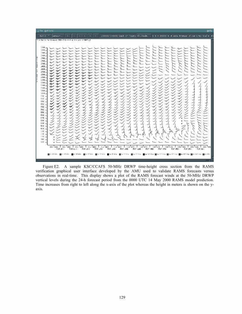
129

Figure E2. A sample KSC/CCAFS 50-MHz DRWP time-height cross section from the RAMS

verification graphical user interface developed by the AMU used to validate RAMS forecasts versus observations in real-time. This display shows a plot of the RAMS forecast winds at the 50-MHz DRWP vertical levels during the 24-h forecast period from the 0000 UTC 14 May 2000 RAMS model prediction. Time increases from right to left along the x-axis of the plot whereas the height in meters is shown on the y-axis.

130

NOTICE

Mention of a copyrighted, trademarked or proprietary product, service, or document does not constitute endorsement thereof by the author, ENSCO, Inc., the AMU, the National Aeronautics and Space Administration, or the United States Government. Any such mention is solely for the purpose of fully informing the reader of the resources used to conduct the work reported herein.