ramos gonzalez, daniel (2021) colour polymorphism in the
TRANSCRIPT

Colour polymorphism in the terrestrial snail Cepaea nemoralis:
from genetics and genomics to spectroscopy and deep learning
Daniel Ramos Gonzalez, MBiolSci
Thesis submitted to the University of Nottingham for the
degree of Doctor of Philosophy
December 2020
Supervisors: Dr. Angus Davison and Dr. Sara Goodacre


i
Thesis abstract
Colour variation in the animal kingdom has been important in science to determine the
principles of biology, especially in genetics and evolution. In the past decades, much
effort has been targeted at the evolutionary, ecological and genetic basis of colour
variation. Although land snails have been relatively neglected, especially in latter
years, a comprehension of genetics and the evolution is important to understand
colour variation precisely because snails may be representative of many species.
When studying colour polymorphism, one of the remaining challenges is to describe
colour. Generally, colour is described manually, relying on the judgment of human
perception, classifying them into a discrete types. The main issue, then, is that human
perception is subjective and colour is continuous. Fortunately, technology has enabled
new techniques to score colour, which may help to investigate colour polymorphism.
This thesis aims to contribute to the knowledge of the maintenance of colour
polymorphism by firstly, understanding the genetics and genomics and secondly,
developing new methods for the scoring of colour. To achieve this, the grove snail
Cepaea nemoralis was selected as a model species. Cepaea nemoralis was chosen
due to their highly polymorphic shell, its easy collection, is widely distributed in all
variety of habitats and the colour and banding morphs showing Mendelian inheritance
(Cain & Sheppard, 1950, Cain & Sheppard, 1952, Cain & Sheppard, 1954, Lamotte,
1959, Jones et al., 1977).
In the first part, I aimed for a better understanding of the inheritance of colour.
Hence, new crosses of C. nemoralis were used, with flanking restriction site–
associated DNA sequencing (RAD-seq) markers used to identify putative instances of
recombination with the supergene that determines colour and banding. No evidence
of the predicted recombinants was found. Instead, a better explanation could involve
incomplete penetrance and epistasis (Gonzalez et al., 2019). The findings therefore
challenge the previous assumption of the supergene architecture and provides a new
resource for the future creation of a fine mapping of the supergene (Gonzalez et al.,
2019).

ii
In the second part, I aimed to understand the evolutionary history of C.
nemoralis, by investigating the relationship of the genomic and supergene variation
with the geographic distribution over Europe. High-throughput genome-wide
genotyping was achieved via a double digest restriction-site associated DNA
sequencing (ddRADseq) method. A broad phylogenomic relationship showed
geographic structure. However, no relationship between the geographical distribution
and colour variation was found. Furthermore, possible genomic regions under
selection, which may be driving the genomic variation, were identified. In addition, the
phylogeny described the evolution of C. nemoralis and indicated how the Pyrenean
lineages colonised Europe after the Pleistocene. The results suggest new roads of
research into the evolutionary and genomic mechanisms that have led the
geographical genomic and supergene variation of C. nemoralis.
In the third part, colour manual scoring was tested using new quantitative
methods to describe colour to better understand colour variation. Therefore, a
comparative study with historical and present shell colour patterns of C. nemoralis in
the Pyrenees was used. Prior studies manually scored shell ground colour into three
discrete colours; yellow, pink or brown. However, colour is continuous and the
description of discrete colours may incur potential error and biased results. Thus, a
quantitative method to score shell colour and to test manual scoring, comparing
patterns of C. nemoralis shell colour polymorphism was used. Similar altitudinal trends
irrespective of the method were found, even though quantitative measures of shell
colour reduced the possibility of error. Moreover, a remarkable stability in the local
shell patterns over five decades were found. This study determined that both methods
remains valuable illustrating several advantages and disadvantages. In the future, a
combination of both methods may be a possible solution.
Finally, and as continuation of the third part, a new visual recognition and
classification method for C. nemoralis based on spectrophotometry and deep learning
was created. Firstly, colour of the shells were quantified by spectrometry, and
secondly, pictures were taken of the measured shells, in different backgrounds. Those
pictures were used to train and test a Region-based Fully Convolutional Networks (R-
FCN). Furthermore, public domain pictures were collected from iNaturalist database
(https://www.inaturalist.org/), to validate the model. The results illustrate that this

iii
method can achieve high accuracy of detection and classification of snails into the
right morph. This work may facilitate the way of how colour polymorphism was
investigated, illustrating new avenues for future research.
In conclusion, this thesis evaluates the limitations found in prior studies and
generates new data for the genetic and genomic understanding of C. nemoralis colour
polymorphism. It also produced viable solutions, using new technologies, to score the
diverse colour morphs. I also contributed to the geographic evolutionary genomic
diversity knowledge.

iv
Publication
Gonzalez, D. R., Aramendia, A. C., & Davison, A. (2019). Recombination within the
Cepaea nemoralis supergene is confounded by incomplete penetrance and epistasis.
Heredity. doi:10.1038/s41437-019-0190-6
Additional manuscripts in review
Ramos‐Gonzalez, D, Davison, A. Qualitative and quantitative methods show stability
in patterns of Cepaea nemoralis shell polymorphism in the Pyrenees over five
decades. Ecol Evol. 2021; 00: 1– 17. https://doi.org/10.1002/ece3.7443

v
Declaration of own work
Although the use of passive voice throughout this thesis have been applied in
agreement of the academic scientific writing, all the practical experiments and data
analysis were conducted by myself, with the exception of clearly mentioned
procedures.
Chapter contributions
Chapter 2: This work was originally conceived by Angus Davison, with the laboratory
work conducted by Amaia Caro Aramendia and myself. The published paper was also
jointly written by Angus Davison and myself.
Chapter 3: This work was originally conceived by myself in discussion with
Angus Davison. The majority of the snails used were collected by Adele Grindon as
part of her PhD. The remainder were collected by a team on a trip to the Pyrenees,
led by myself and with the help of Angus Davison, Hannah Jackson and Alejandro
Garcia Alvarez. The unpublished reference genome was kindly provided by Suzanne
Saenko. The analysis was carried out by myself, in discussion with Angus Davison.
The work was first drafted by myself, and then reviewed by Angus Davison.
Chapter 4: This work, including the sampling design and the comparison
between qualitative and quantitative methods, was originally conceived by myself in
discussion with Angus Davison. The Pyrenean samples were collected by a team led
by myself, with the help of Angus Davison, Hannah Jackson and Alejandro Garcia
Alvarez. The analysis was carried out by myself, in discussion with Angus Davison.
The work was first drafted by myself, and then reviewed by Angus Davison.
Chapter 5: This work was originally conceived by myself, in discussion with
Angus Davison and Alejandro Garcia Alvarez. All images were generated by myself.
The deep learning algorithm was developed by Alejandro Garcia Alvarez, in discussion
with me. The analysis was carried out and the work was first drafted by myself, and
then reviewed by Angus Davison.

vi
Acknowledgements
The completion of this thesis has been possible to a great extent by the guidance,
help, collaboration and moral support of many people, both in Nottingham and
elsewhere on the planet. First and foremost, I would like to thanks to my supervisor
Dr. Angus Davison. I really appreciate your understanding, guidance and attention
from the first days to the last of this PhD. I also would like to thanks Dr. Sara Goodacre,
the members of the staff and all the other students and academics for showing support
and invaluable experiences, when I most needed it.
Moreover, I would like to thanks University of Nottingham and the
Biotechnology and Biological Sciences Doctoral Training Programme to give me the
chance, first, and the financial support and resources to accomplish this thesis.
A special thanks to Alejandro Garcia Alvarez for joining my fieldwork expedition
to the Pyrenees, for providing guidance in the development of the deep learning
algorithm and for the moral support. I also would like to thanks to Hannah Jackson for
joining my fieldwork expedition to the Pyrenees. Thanks to both Sheila Keeble and
Julie Rodgers for help with the care of snails, to Amaia Caro Aramendia to contribute
in the genotyping of the snail crosses and to Sophie Poole who helped with some of
the shell colour measurements. Thanks to the SNPsaurus team to deliver the RAD-
sequencing. Moreover, the analysis of the genomic data would have not been possible
without the guidance of Dr. Mark Ravinet, Dr. Joana Meier and Dr. Simon Martin.
I would also like to thanks to Jonathan Silvertown and the Evolution Megalab
team who provided the historical data used in the comparative study. thanks to Dr.
Adele Grindon for providing the European sampling collection and Dr. Suzanne
Saenko who provided an unpublished Cepaea nemoralis reference genome. Also,
thanks to Dr. Laurence Cook as well as three anonymous referees for comments on
the genetics manuscript, and to Dr. Robert Cameron and Dr. Małgorzata Ożgo for
comments on the Pyrenean chapter. Additionally, to Anne Clarke and the University
of Nottingham for access to the archive of Professor Bryan Clarke.

vii
Finally, I would like to express my endless gratitude to my family, especially to
my mother Marisa Gonzalez Ventoso, my sister Judit Ramos Gonzalez, my
grandmother Maria Luisa Ventoso Bofill, my uncle Juanjo Gonzalez Ventoso, my
cousins and my aunt-cousin Hortensia Gonzalez de la Fuente, for being just the nicest
people ever. Also thanks to Noemi Contreras Marmol for caring and supporting me,
Marc Gallardo Lombarte to keep me fit, Carlos Dominguez Puig because of his
“repechitos”, Adrian Perez Martinez because of his resilient encouragement, Isaac
Vidal Valdivia and his medical approach to live, Cristian Bejarano del Olmo due to his
life challenges, Guillermo Arranz Bernal to teach me how to relax and many others to
believe in me. To the DTP crew, especially Pierre Reitzer and his board-game nights,
James Reekes and his runs at Uni park and Nottingham handball club to make these
four years fantastic. Ultimately, thanks to my supportive bubble during this lockdown
times, Giada Pedretti and her plank challenges, Louise Nathalie Vingert Silveira and
her coffee breaks and excellent motivation, Samantha Paterson and the cow vision of
life, Fotini Iacovou keeping my feet in the ground, Mark Palmieri and his Italian way of
life and Bruna Falgueras Vallbona for your hope, your energy, your joy and your great
support.
“In the long history of humankind (and animal kind, too) those who learned to
collaborate and improvise most effectively have prevailed.”― Charles Darwin, The
descent of man, 1871.

viii
List of figures
1.1. C. nemoralis illustration 8
1.2. CIE 1931 chromaticity diagram 16
2.1. Representation of shell offspring and putative recombinant 34
3.1. European map of the genomic sampling collection 47
3.2. Genomic structure of C. nemoralis across Europe 54
3.3. Correlation of Fst versus geography 58
3.4. Density graphs of genetic differentiation 59
3.5. PCA analysis to the supergene-linked dataset 65
4.1. Overview of Pyrenean sampling locations 76
4.2. Colour distribution in the Central Pyrenees 82
4.3. Banding distribution in the Central Pyrenees 83
4.4. Comparison of changes in the shell frequencies 85
4.5. Present-day relationship of shell features and altitude 87
4.6. PC3 and altitude relationship 89
4.7. Relationship between altitude and colour variation 91
5.1. Bounding box pictures 107
5.2. General organization of R-FCN 109
5.3. Prediction result examples 112
5.4. Examples of prediction failures 113
5.5. Prediction test results 115
5.6. Background accuracy results 116
5.7. Pink banded variation 120
List of tables
2.1. Phenotypes and genotypes of C. nemoralis crosses 26
2.2. Summary of linked loci phenotypes 29
2.3. Summary of RAD-seq markers genotyping 37
3.1. Genomic samples summary 48
3.2. Four population test (D-statistic) results 56
3.3. Fst mean between all populations comparisons 60
3.4. Genbank homology sequences 63

ix
4.1. Sampling collection summary 80
4.2. Statistical summary of shell geographical distribution 84
4.3. Fisher r-to z-transformation summary 88
5.1. Summary of picture datasets 104
5.2. Summary of accuracy metrics 114

Table contents
Thesis Abstract i
Publication iv
Additional manuscripts in review iv
Declaration of own work v
Chapter contributions v
Acknowledgements vi
List of figures viii
List of tables viii
Chapter 1: General introduction 1
1.1. Evolutionary genetics and genetic polymorphism 1
1.2. The grove snail (Cepaea nemoralis) in evolutionary genetics 4
1.3. Synthesis of the genetics and genomics of C. nemoralis 9
1.4.Characterising colour polymorphism 15
1.5. Citizen science 18
1.6. Thesis aims 19
Chapter 2: Recombination within the Cepaea nemoralis supergene is
confounded by incomplete penetrance 22
Abstract 22
2.1. Introduction 23
2.2. Materials and methods 25
2.2.1. The culture of Cepaea and crosses 25
2.2.2. DNA extraction, quantification and amplification 30
2.3. Results 32
2.3.1. Segregation of Mendelian loci that determine shell phenotype 32
2.3.2. Putative recombinants between colour, banding and lip and band
pigmentation loci 33
2.3.3. Genotyping of offspring using RAD-seq derived loci 36
2.4. Discussion 38
2.4.1. Incomplete penetrance and epistasis 38
2.4.2. Future progress 41
2.5. Acknowledgements 41

Chapter 3: Exploring the divergence of genomic variation and geographical
structure in Cepaea nemoralis 42
Abstract 42
3.1. Introduction 43
3.2. Materials and Methods 47
3.2.1. Dataset collection 47
3.2.2. Genomic methods 50
3.2.3. Sequence analysis and datasets 50
3.2.4. Analyses of genomic variation 51
3.3. Results 53
3.3.1. Western European phylogenomics of C. nemoralis 53
3.3.2. Different genomic evolutionary history of the colour and geographic
variation 64
3.4. Discussion 66
3.4.1. Colour and genomic geographic variation 67
3.4.2. Evolutionary history, genomic diversity and population structure of C.
nemoralis 69
3.5. Acknowledgments 71
Chapter 4: Qualitative and quantitative methods show stasis in patterns of
Cepaea nemoralis shell colour polymorphism in the Pyrenees over five
decades 72
Abstract 72
4.1. Introduction 74
4.2. Materials and methods 77
4.2.1. Shell samples and human-scoring of shell phenotypes 77
4.2.2. Quantification of shell colour 78
4.2.3. Analysis of phenotype frequencies and correlation 79
4.3. Results 80
4.3.1. Past and present-day geographic distribution of colour and banding
morphs 80
4.3.2. Quantitative measures of shell colour and banding and associations with
altitude 88
4.3.3. Past and present-day associations, using qualitative and quantitative
methods 89
4.4. Discussion 92
4.4.1. Quantitative versus qualitative methods to score shell phenotype 92
4.4.2. Past and present-day geographic distribution of colour and banding
morphs 93
4.4.3. From phenotype to genotype 94
4.4.4. Conclusion 95
4.5. Acknowledgements 96
Chapter 5: A new C. nemoralis recognition and shell morph classification
system using deep learning 97
Abstract 97
5.1. Introduction 98
5.2. Materials and methods 102
5.2.1. Image datasets 102
5.2.2. Training inputs 106
5.2.3. System overview 108
5.3. Results 111
5.4. Discussion 117
5.5. Conclusion 121
5.6. Acknowledgements 121
Chapter 6: General discussion and conclusions 122
6.1. Cepaea nemoralis colour polymorphism, a multidisciplinary challenge 122
6.2. Future steps towards understanding Cepaea nemoralis shell polymorphism
125
6.2.1. Mapping Cepaea nemoralis genome 125
6.2.2. Citizen science, the future of ecological and evolutionary genetics 128
6.3. Final conclusion 132
References 135
Supporting information 150
Chapter 2 150
Chapter 3 169
Chapter 4 218

Chapter 5 238

1
Chapter 1:
General introduction
1.1. Evolutionary genetics and genetic polymorphism
Historically, ecological and evolutionary genetics studies have focussed on two
patterns found in nature: adaptation, which refers to the relationship of the “fit” between
environment and individuals, and genetic polymorphism (Dobzhansky et al., 1970). In
the natural world, a genetic polymorphism occurs when phenotypic variation within
and between populations of the same species is maintained and caused by two or
more alleles each with considerable recurrence (Ford, 1975). Thus, ecological and
evolutionary genetic studies focus on changes in the frequency of genotypes within
populations, which ultimately may lead to speciation. Hence, the longstanding aim in
evolutionary genetics has been to understand how the evolutionary factors affect the
variation of biodiversity observed in nature.
There are four main evolutionary forces acting among and within populations
of the same species: random genetic drift, gene flow, natural selection and mutation.
Random genetic drift occurs in any population of finite size, due to random sampling
of individuals (Masel, 2011; Wright, 1937), with smaller populations more affected.
This effect is most pronounced in a bottleneck or founder event (Star et al., 2013;
Wright, 1937). Gene flow is defined as the transmission of genetic material among
populations. Normally, this event is caused by migration between populations (Star et
al., 2013). In the case of populations illustrating high levels of genetic material
transmission with similar allele frequencies, both populations can be considered as a
single population. Natural selection pressures are described as the survival and the
production of offspring to some individuals displaying specific morphs within
populations due to their more adapted features for those environmental conditions
(Darwin, 1859; Star et al., 2013). Finally, mutations are modifications in the DNA
sequence of the genome of an individual (Beadle et al., 1941).

2
These evolutionary forces vary in their influence upon populations. While the
majority of genetic mutations are neutral, which means that they do not have either
positive or negative effects on the fitness of the individuals (Ford, 1975), when a
positive or negative mutation occurs, other factors are known to act. For example, the
pressure of directional selection often may cause that a new active genetic mutations
becomes widespread over long periods due to ‘survival of the fittest’ (Wade, 2008), or
random genetic drift may also contribute to the increase of the new active genetic
mutations. However, also other forces may challenge the new effective genetic
mutations. For instance, high levels of gene flow may contribute to the maintenance
of the previous characteristics of the species. The higher the migratory frequency, the
greater the probabilities of maintaining pre-established genetic conditions (Star et al.,
2013). These evolutionary processes can interact and oppose each other as they may
operate simultaneously causing alterations in the allele frequencies (Svensson, 2017).
All these factors can be determined by mathematical theories of population genetics,
which were generated by examining the evolutionary forces effects on genetic
variation in species (Cook et al., 1996; Fisher, 1947; Ford, 1975; Wright, 1948).
In addition, there are other evolutionary process causing genetic polymorphism
besides the genetic drift and directional selection. For example, frequency-dependent
selection, which the fitness of the genotype depends on their abundance in the given
population, may increase the frequency of rare morphs (Ayala et al., 1974; Jones et
al., 1977). Either disruptive selection, which favours the extreme types of a normal
distribution in a population as a consequence of a balance between gene flow among
subpopulations and natural selection acting in diverse directions (Jones et al., 1977).
Alternatively, also heterozygous advantage (stabilizing selection), which the
heterozygote morph are fitter than the homozygote ones (Cain et al., 1963; Cain et al.,
1954; Jones et al., 1977).
The emphasis of past research has been on attempting to determine whether
polymorphism was genetic or not, the identification of each morph frequency and
understanding its maintenance by examining natural selection and other evolutionary
factors acting upon it (Fisher, 1930; Ford, 1975). During the beginning of the past
century, the earliest ecological geneticists primary aim was to target natural selection
as the main justification to explain the maintenance of a balanced polymorphism,

3
which is the coexistence and constancy of frequencies of several morphs in a given
population (Fisher, 1930; Ford, 1975). Therefore, selective forces such as climate
selection, predation or habitat were considered the main interpretation to explain
morph frequency variation. For example, in the land snails Theba pisana, the
absorption of heat by exposure to the sun by their shells depended on the colour, with
the lighter colours absorbing the least heat (Cain, 1984; Cowie, 1990; Scheil et al.,
2012a). Moreover, predation and habitat, together, can play a key role in the
distribution of shell morphs, creating a mosaic of different frequencies among
neighbouring populations (Cain, 1984; Cowie, 1990; Heller, 1981; Scheil et al., 2012a).
The song thrush (Turdus philomelos) is known as one of the main predators of Theba
pisana discriminating conspicuous shells depending on the background (Heller, 1981).
For example, lighter shells in darker backgrounds are more exposed to predation
affecting the fitness of the morphs (Johnson, 2011).
Then, from the 1960s and subsequent years, the introduction of molecular
biology techniques changed the field of evolutionary genetics, raising new questions.
As a result, researchers started focusing on understanding the genetic inheritance and
genetic and genomic patterns driving the polymorphism. In recent decades, as DNA
sequencing became more accurate, efficient and widely available to all researchers,
novel methodologies were created, which opened up more precise conclusions. For
instance in evolutionary biology, genome-wide sequencing is used to investigate
complex evolutionary processes. For example in the House sparrows (Passer
domesticus), this technology helped to comprehend the causes of new rapid genetic
adaptations due to links with human development (Ravinet et al., 2018).
Among all kinds of polymorphism found in nature, one of the most studied is
colour polymorphism. Traditionally, colour polymorphism was used to understand the
functional meaning and ecological circumstances of all morphs due to the ease of
recognising and describing their different phenotypes (Svensson, 2017). For example,
some of the most common species used were butterflies and snails. These species
exhibited clear visible phenotypic variation and can easily be raised in captivity, which
made them model species in the earlier studies of natural selection (Fisher, 1930;
Müller, 1879).

4
There are many examples of colour polymorphic model species. One of the
classic colour polymorphic model species are the butterflies with mimicry rings (e.g.
Heliconius numata and Consul fabius) (Müller, 1879). These species have been
broadly studied to determine, for example, natural selection, aposematic selection, in
which some morphs mimic dangerous or distasteful species for the predator (Joron et
al., 1998), or to test gene flow and speciation (Martin et al., 2013). Another classic
example used in evolutionary and ecological genetics is the Scarlet tiger moth
(Panaxia dominula). P. dominula displays wing colour variation from a metallic-green
sheen with white and orange or yellow signs, to red hindwings with variable black
marks. This species was a target of one of the longest and continuous surveys in a
single population (Fisher, 1947). Fisher (1947) examined possible annual fluctuations
in morph frequency variation of P. dominula to explain whether natural selection of
random genetic drift showed more influence in those changes. Fisher found that the
observed fluctuations were driven by natural selection concluding that selection could
be tested in wild populations (Fisher, 1947).
Other species, such as avian model species have also been at the centre of
evolutionary research. For instance, hundreds of bird species including Strigiformes,
Ciconiiformes, Cuculiformes and Galliformes, which show a range of colour
polymorphic plumage (Galeotti et al., 2003) are used to understand the maintenance
of the polymorphism due to its variety of possible selective scenarios where birds can
be prey, predators and competitors at the same time. In this case, in evolutionary
genetics, birds became model species, for example, to comprehend selection (Clarke,
1969; Paulson, 1973), to study disruptive selection (Baker et al., 1979; Rohwer, 1990),
or to determine sexual selection among individuals (Endler, 1987).
1.2. The grove snail (Cepaea nemoralis) in evolutionary genetics
Terrestrial land snails can be considered as rather inconspicuous fauna in nature.
However, some snail taxa exhibit an extensive shell variation, from patterning, shell
shape or chirality to ground colour, making them useful to study genetic polymorphism.
Studies focused on the genetic mechanisms and micro-evolutionary events caused by

5
selective factors in land snail species have been carried out over a century. With the
main aim to understand the evolution and maintenance of shell polymorphism.
Land snails have, undoubtedly, played an important role in understanding
genetic polymorphism resulting into the establishment of the modern ecological and
evolutionary genetic discipline (Murray et al., 1978). Previous to the modern
evolutionary synthesis, a great variety of studies were carried out based on the
acquisition of the intrinsic knowledge of shell polymorphism. For example, land snail
genera such as Theba, Trochulus, Partula or Cepaea (Clarke et al., 1971; Jones et
al., 1977; Proćków et al., 2018; Scheil et al., 2012b), with a huge range of colour and
banding shell patterns, were selected as models to understand its mechanisms. In
French Polynesia the Partula genus was surveyed in the search of the understanding
of the selective forces acting upon its shell colour variation (Clarke et al., 1971).
Furthermore, recent research examples in land snails showed how colour and its
thermic capacities of heat absorption are involved in Theba pisana shell variation,
illustrating a correlation between shell type distribution and climatic selection (Scheil
et al., 2012b); or habitat and shell morphology relations in the European Trochulus
hispidus and Trochulus sericeus (Proćków et al., 2018).
In particular, the famous land snail Cepaea nemoralis was perceived as an
excellent model species to study colour polymorphism due to its apparent non-
adaptive and random diversity in wild populations (Lamotte, 1951). As mentioned
above, the classic studies examined whether natural selection prevailed as the
principal cause of shell banding and colour variation (Cain et al., 1950, 1952, 1954).
Thereafter, other comparative surveys brought out other selective factors such as
predation, variety of habitats and other evolutionary forces illustrating correlations with
shell morph frequencies (Jones et al., 1977). Nowadays, C. nemoralis has became a
traditional case study of adaptive evolution, attracting a growing interest from both,
professionals and citizen scientists (Chapters 4 and 5; Cameron et al., 2012; Kerstes
et al., 2019; Silvertown et al., 2011). Additionally, the development of new molecular
protocols brings new avenues in the understanding of evolutionary forces and non-
selective mechanisms related to the roots of natural variation in terrestrial land snails
(Davison, 2002; Richards et al., 2013).

6
Overall, C. nemoralis is a good case to study in evolutionary genetics for a
broad range of reasons (Figure 1.1). Firstly, it occupies a variety of different habitats,
from woodland and grassland to sand dunes (Jones et al., 1977). Secondly, simple
Mendelian inheritance is shown in the major loci that establishes shell polymorphism
(Chapter 2 and 3; Cook, 1967; Jones et al., 1977). Thirdly, it has a highly polymorphic
shell, which show three main inherited features. On one side, shell ground colour (C)
can be dark brown, pink or yellow with deduced genotype dominance (brown > pink >
yellow). On the other side, shells may have a wide range of dark bands (B) from zero
to five, with its deduced genotype dominance (absence > presence). Moreover, bands
may differ in their pigmentation (P), usually being fully pigmented bands, but
sometimes unpigmented, interrupted (I), or spread (S). The genotypic dominance, in
this case, being normal pigmentation dominant (Chapter 2, 3, 4 and 5; Jones et al.,
1977). Fourthly, shape and coiling illustrate clear variation. All these traits together
may be associated with environmental parameters and their intrinsic genetics can be
a possible practical genetic marker themselves, which are genes with known location
that can be used to recognise species (Figure 1.1, Davison, 2002; Murray et al., 1978).
Finally, C. nemoralis can sometimes be crossed to obtain offspring and are easily
maintained in laboratory. This is certainly helpful in the molecular studies (Davison,
2002; Richards et al., 2013).
In addition, at least nine loci involved in the expression of shell polymorphism
have been identified, from which at least five are considered to be tightly linked
together into a ‘supergene’ (Jones et al., 1977; Richards et al., 1975; Richards et al.,
2013), a supergene is a group of neighbouring genes that inherited together (Ernst,
1936). Consequently, band presence, ground colour, pigmentation, interruption and
fusion are thought to be linked in the supergene. Moreover, band suppression, which
is supposed to have two loci, the intensity and colour banding seems to be unlinked
loci (Richards et al., 2013). All these loci showed epistatic interactions among them
and with the unlinked loci. Furthermore, the recombination frequencies within the C.
nemoralis supergene have been estimated empirically (Cain et al., 1960; Cook, 1967;
Richards et al., 2013). The conclusions hypothesised of a very tight linkage cluster
composed by shell ground colour, band presence and band interruption showing
recombination rates of ~0–2%. Other loci such as the spread banding and band
pigmentation may be slightly loss than the C‐B linkage cluster, with respective

7
recombination rate estimations of ~3–4% and ~4–15% (Cain et al., 1960; Cook, 1967;
Richards et al., 2013). Finally, Richards 2013 were able to generate RAD markers
linked to the C. nemoralis supergene creating the basis for forthcoming research in
molecular ecology.
In addition, museums, universities and digitised projects recorded and stored
an abundant historical data from the 20th century on C. nemoralis, which continue to
be available to the modern days (Silvertown et al., 2011).

8
Figure 1.1. Illustration of the variation of Cepaea nemoralis shell colour and banding in wild-collected individuals.

9
1.3. Synthesis of the genetics and genomics of C. nemoralis
As mentioned above, the historical evolutionary processes of colour polymorphic
species have been a focus of research in evolutionary biology. One common approach
to contribute to the study of colour polymorphism is the use of molecular biology
methods due to their many attributes as mention in section 1.1 of this chapter (Cuthill
et al., 2017; McKinnon et al., 2010; McLean et al., 2014; San-Jose et al., 2017). The
objective of molecular biology in polymorphic evolutionary genetics, therefore, is to
understand the molecular mechanisms and processes driving the evolution and
maintenance of polymorphisms.
Pulmonate snails, like the genus Cepaea, have been presented as good model
species candidates when researching environmental and evolutionary genetics due to
the abundance of ecological data as also reviewed in section 1.2 of this chapter
(Davison, 2002). Many efforts have been made in the understanding of the historical
evolutionary processes of C. nemoralis. However, only a small number of studies
used genetic data, even though molecular biology research in evolutionary biology
and especially in evolutionary genetics started in the 1960’s. Historically, the study of
the maintenance of C. nemoralis colour polymorphism were based on the generation
of crosses, and comparative surveys (morph frequencies) rather than molecular
research, which were and are commonly used to create a broad picture of the
understanding of the maintenance of the polymorphism. Originally, the shell morph
diversity was thought to be non-adaptive and due to local events (Cameron, 1998;
Goodhart, 1963). Nonetheless, the following 30 years of morph frequency research
concluded that the shell polymorphism was, indeed, adaptive and that their morph
frequencies could be influenced by natural selection (Jones et al., 1977). These
studies provided important knowledge and insights on how evolutionary forces
influence populations in local or larger areas. However, there are many unresolved
questions, which need to be investigated from other perspectives.
In subsequent years, molecular population genetics was revolutionised by the
development of genetic data collections and subsequently, academic developments.
These new developments allowed the first measures of genetic variation in C.

10
nemoralis, to occur using alloenzymatic and enzymatic loci, opening a new era of
research in population genetics. These studies enabled researchers to assess
differences between adjacent populations contributing to their understanding of the
evolutionary history, gene flow and selection in ‘area effects’ cases (Johnson, 1976;
Ochman et al., 1983). The term ‘area effects’ is associated to the Cepaea genus and
refers to the stability of morph frequencies over extensions bigger than a panmictic
unit despite the visual selection, which these effects are caused by selective forces
not related directly to the topography (Cain et al., 1963). For example, in the Pyrenees,
where Caugant et al. (1982) and Ochman et al. (1983) sampled the region and
generated local phylogenies using enzymatic variation, both authors identified a
polymorphic morphological and molecular geographic structure in Pyrenean
populations due to ‘area effects’. Their findings suggested that the described ‘area
effects’ were due to the temporary geographic isolation during the last glaciation.
Subsequently, Valdez et al. (1988) and Guiller et al. (1993) sampled the same and
other areas of the Pyrenees with similar hypothesis, results and conclusions reported.
Other authors used enzymatic variation to evaluate ‘area effects’ in other geographical
regions. For example in the Lambourn Downs, Johnson (1976) hypothesised of
several causes of ‘area effects’ found due to lack of evidences not giving a clear
explanation of the patterns found (Johnson, 1976). Another study in the lowlands of
England used molecular enzymatic variation to test ‘area effects’ by visual selection in
C. nemoralis populations finding instead, a correlation with altitude (Wilson, 1996).
Moreover, the employment of mtDNA and small numbers of genetic markers to
assess phylogenetic relationships started to be used in evolutionary biology. In C.
nemoralis, molecular biological studies aimed to understand either the genetic
inheritance of C. nemoralis (Davison, 2000b; Terrett et al., 1996; Thomaz et al., 1996;
Yamazaki et al., 1997), or whether to infer the genetic evolutionary history and the
factors acting within and between populations (Davison, 1999, 2000a; Davison et al.,
2000; Ellis, 2004; Grindon et al., 2013a; Neiber et al., 2015). For example, Davison, in
a series of consecutive studies, performed the first few studies based on genetic data
in C. nemoralis (Davison, 1999, 2000a, 2000b; Davison et al., 2000). Initially, the first
microsatellite primers and mtDNA (16S rRNA locus) were created for C. nemoralis
individuals striving to set the foundation for future research in the population
relationships of the grove snails (Davison, 1999, 2000b). Subsequently, the

11
microsatellite and the mitochondrial DNA were used to assess ‘mysterious’
geographical patterns of shell polymorphism both locally in the famous Marlborough
Downs in Wiltshire (Davison et al., 2000). As well as a more broadly study to evaluate
the distribution of C. nemoralis from East to West in the islands of Britain and Ireland
finding that the origin of the Irish populations may not come from the Britain island
(Davison, 2000a). Moreover, mtDNA was used to infer the mitochondrial genomic
inheritance discarding the possibility of a doubly uniparental inheritance, as it happens
in other species like Mytilus, where maternal and paternal mitochondrial lineages
coexist (Garrido-Ramos et al., 1998).
Furthermore, various authors used the molecular variation in C. nemoralis
mitochondrial DNA to infer the genetic geographic divergence in European
populations. In a notable example, Neiber et al. (2015) generated a molecular
phylogeny combining mtDNA and nuclear sequences to study the ancestry of the
genus Cepaea. The Cepaea genus was thought to be monophyletic and comprised of
four pulmonate species; C. nemoralis, C. hortensis “Cepaea sylvatica” and “Cepaea
vindobonensis”. However, molecular phylogeny, using mitochondrial and nuclear
sequences and comparing to another 20 genera of Helicidae, revealed that the
supposed Cepaea genus is polyphyletic and that C. sylvatica is more closely related
to Macularia genus and C. vindobonensis to the genus Caucasotachea (Neiber et al.,
2015). Complementary, other research using mtDNA of just C. nemoralis populations,
helped to reveal the expansion of snail populations after the Pleistocene. For instance,
Grindon et al. (2013a) surveyed Europe to determinate the Irish ancestry using C.
nemoralis. Interestingly, a mitochondrial lineage (C) was found only in the central and
Eastern Pyrenees, Ireland, the western area of Great Britain and the Isle of Man.
Grindon et al. (2013a) argued that vessels brought these populations through the
Noguera Pallaresa – Garonne River to the Irish island, from the Pyrenees. In addition,
Ellis (2004) evaluated the molecular pattern distribution of C. nemoralis populations in
a local area, the Pyrenees. In this instance, mitochondrial DNA together with
enzymatic variation were used to examine the relationship of shell patterns with their
geographic distribution. Due to a lack of association, therefore, Ellis (2004) argued
that the molecular and shell pattern variations were likely “relics of history” rather than
variations caused by molecular area effects.

12
Whereas the use of few genetic markers and mtDNA have undoubtedly been
informative when testing phylogenetic associations. The use of these methods has
revealed several limitations. Firstly, mapping single genes may generate variations
from the general species phylogeny (Nichols, 2001); biased results may occur due to
many reasons such as population level relationships, bottlenecks, high mutation rates,
introgression or to the low representation of the species when using individual or few
genes. This is consistent with Davison et al. (2000) who showed how genetic markers
could differ among them due to events like ‘area effects’. Secondly, even though
mtDNA can add information in the study of the genetic variation, it needs to be taken
cautiously. As Funk et al. (2003) reported, mtDNA phylogenies can be strongly
influenced by incomplete lineage sorting and introgression at species level. Thirdly,
positive selection on mtDNA may affect the neutrality of known genetic markers as
Parmakelis et al. (2013) indicated. Finally, and specifically in pulmonate snails, the
rate of mtDNA evolution is remarkably elevated compared to other animal families
(Thomaz et al., 1996), making outcomes uncertain. Previously, several authors
thought that this mtDNA high rate was due to result of selection, high mutation rate or
even population demography (Davison, 2002; Thomaz et al., 1996). However, these
explanations may be insufficient to explain the high mitochondrial genetic diversity in
pulmonate snail rising the ovotestis effect. The ovotestis effect occurs in
hermaphrodite species where both reproductive cells (ova and sperm) accumulated
similar mutation frequency increasing the mtDNA diversity (Davison, 2006). This
hypothesis is founded in the theory of both reproductive cells undergo to approximately
the same cell divisions showing similar accumulated mutation rates (Davison, 2006).
Currently, evolutionary genetics is entering an interesting prolific period.
Technological progress in population-scale sequencing are developing rapidly. They
are driving scientists to useful data sources, which are influencing and transforming
the studies in genetic polymorphism. Consequentially, recent studies in C. nemoralis
started using population genomics, proteomics, and transcriptomics and epigenomics
techniques. All these molecular procedures enhance the knowledge of microevolution
in individuals contributing to determine the demography of a population and its
phylogenetic history. Thus, the use of one or another method depends on the
hypothesis being tested. For instance, proteomics is frequently used to understand the
expression of pigments. In molluscs, there are a lot marine snail shell-proteomes

13
characterised (Kocot et al., 2016). In land snails, next generation sequencing and high
throughput proteomics has been used to characterise the first pulmonate of Cepaea
nemoralis shell-proteome (Mann et al., 2014). The advantage of using proteomics
instead of transcriptomics to describe a protein is that transcriptomics gives a rough
estimation of the protein expression while proteomics confirms and quantifies the
presence of a protein.
Moreover, the transcriptomics high-throughput method to study the genome are
useful to unravel local adaptation processes in several time and temporal scales
(Hendricks et al., 2018). Recent advances in RNA-seq library techniques provides
accurate measurement of transcription, increases the use of transcriptomic analysis
and enhances the accessibility of these methods to ecological and evolutionary
studies (Stahlke et al., 2020). However, they are still in the development process due
to technical limitations such as high-quality RNA isolation, pooling samples or the
balance between biological replications and sequencing depth, demonstrating,
nonetheless, good potential in the future for studies of population genomics (Le Luyer
et al., 2017; Lim et al., 2020; Stahlke et al., 2020). These methods are widely used,
for example, to identify changes in gene expression to enable adaptation to different
environmental conditions in species such as Oncorhynchus mykiss gardieri known as
redband rainbow trout (Chen et al., 2018; Garvin et al., 2015) or corals (Bay et al.,
2017; Pratlong et al., 2015). In the case of C. nemoralis, transcriptomics has been
used to identify and validate reference genes, and in particular, the candidate genes
involved in shell colour polymorphism (Affenzeller et al., 2018; Kerkvliet et al., 2017).
Finally, whole genome sequencing and reduced representation methods such
as restriction-site associated DNA-sequencing (RADseq) have grown as a common
methodology in this field (Hohenlohe et al., 2018). Genomic variation in species is
caused by many factors having an effect among and within populations of a particular
species. These technologies, therefore, offer the possibility to investigate extrinsic and
intrinsic forces equally (Campbell et al., 2018). Thus, detailed questions such as inter
and intra population interactions or genome architecture can be approached to find
out which forces drive these effects. Moreover, while past genetic techniques
generated limitations when building phylogenies due to strong biases results found
using limited number of genetic markers as stated above, the availability of generating

14
de novo genome assemblies and the access to a growing number of already
sequenced reference genomes will help overcome biased results (Campbell et al.,
2018). Finally, the genomic architecture generated using genome-scale data may
bring solutions to unresolved questions when genetic-scale data and transcriptomics
cannot answer the cause of polymorphic frequency stasis or divergence. To date,
there have been only two studies using genomic data in C. nemoralis (Richards et al.,
2013; Saenko et al., 2020). In one, Richards 2013 used RAD-seq sequencing to flank
and create genetic markers to the shell colour and banding supergene aiming at
helping future genome mapping (Richards et al., 2013). In the other one, Saenko et
al. (2020) build the first draft of a reference genome of the target species.
The field of genetic and genomic studies is growing, becoming richer and more
complex. Thanks to that, researchers are able to find, describe and understand the
interplay among processes, patterns and features of the genome, together with
ecological factors of the species. It is definitely becoming clear that the study of
ecological evolutionary genetics is more complicated than analysing one single factor
and that the field will push towards future multidisciplinary insights into natural, non-
model populations stories throughout the Tree of Life.
15
1.4. Characterising colour polymorphism
The study of animal colouration has been a crucial part in the comprehension of the
biological fundaments in ecology, evolution and biology (Cuthill et al., 2017; McKinnon
et al., 2010; McLean et al., 2014; San-Jose et al., 2017). Colour in biology emerges
from a combination of nanoparticles and pigments (Stuart-Fox et al., 2018), being in
species a complex attribute to describe. Colour is, therefore, remarkably visible but at
the same time complex to understand. Sometimes, it is easy to identify colour in nature
and relate it with species evolution, production and function. Other times, colour can
be a complicated feature to use in the recognition of species. In land snails, for
example, colour is fundamental in the thermoregulation of species. Lighter shell
colours may survive better in hotter areas due to lighter shell colours absorbing less
radiation compared with darker shells (Cameron et al., 2013; Mazon et al., 1987;
Ramos, 1984; Richardson, 1974). In birds, colour is also known to play a crucial rule
in sexual selection. For instance, colourful plumage is used in signalling of courtship
(Galeotti et al., 2003).
However, even though colour is easy to spot, it is difficult to describe and
quantify. Colour is a quality, which can be described by its lightness, saturation and
hue. Isaac Newton was the first scientist to demonstrate in his prism experiment, that
the colour was a consequence of reflectance spectra. He also described the continuity
of colour, rejecting the theory of the existence of discrete colours (de Andrade Martins
et al., 2001). Besides, colour also depends on the visual perception of the receptor
involving physics, psychology and physiology. In the animal kingdom, each species
has different mechanisms to process colours, and within species, each individual
perceives colours differently. For example, birds have four different photoreceptor cell
types to perceive colour with different sensitivities; long (L), medium (M), short (S),
and very short (VS), which all together generate a tetrachromatic colorimetric system
(Davison et al., 2019a; Delhey et al., 2015). By contrast, humans possess three groups
of photoreceptor cells in the retina: L (long wavelength, peaking at 560 nm), M
(medium wavelength, peaking at 530 nm), and S (short wavelength, peaking at 420
nm) (Chapter 5, Hunt, 2004). For humans, the International Commission on
Illumination (CIE), created the foundations to define the human colorimetric system,

16
based on the stimulation of the different photoreceptor cells of the retina (Smith et al.,
1931; Westland et al., 2012).
Figure 1.2. The chromaticity diagram system of the CIE 1931 colour convention. Wavelengths
measured in nanometres illustrated the spectral boundary curved (monochromatic) locus. Colours
shown in the diagram are translated into RGB chromaticity coordinates. The diagram was made using
Pavo 2.2.0 R package in R version 3.4.1 (2017-06-30).
Since the 1931 convention (CIE), the definition of chromaticity is determined by
the quantitative distributions of wavelengths in the visible spectrum (Figure 1.2).
Colour-space mathematical equations are the basis to quantify the spectra and
translate into the human chromatic visible spectrum to further test colour variation. As
mentioned above, the human visual is captured by three different cone cells. Thus, the
CIE commission agreed on three parameters representing each type of cone cells
called the Tristimulus values (XYZ). This system corresponds to the primary colours,
red, green and blue, and is based on an observer’s point of view, which was
standardised to the 2o arc of the fovea to reduce the number of variables (Smith et al.,
1931; Westland et al., 2012). These Tristimulus values provide a standard reference
to other colour spaces such as the well-known RGB (red, green and blue), CIE-LAB
(abbreviated as Lab) and, HSV (hue and saturation value).

17
Throughout the past century, biological studies involving colour features were
scored manually, using the expert perception of a trained biologist. Traditionally, in the
ecological and evolutionary genetics fields, colour description has been subjective.
For instance, pure genetic studies, demonstrating the basic Mendelian genetic
theories in species (Staples‐Browne, 1908; Wheldale, 1907), or biogeographic
surveys aiming to deduce natural and sexual selection operating in nature (Delhey et
al., 2015; Delhey et al., 2017) used manual scoring instead of quantitative methods
(Endler, 1990). This may lead to potential error and biased results when scoring
colour. The next step was to move to quantitative colour descriptions by using
quantitative procedures. Thus, spectrophotometry rose as one of the most accurate
and sophisticated tools to approach this issue. Spectrophotometry exposes objects to
a certain light and compares the amount of light emitted to that received.
Consequently, it measures the light absorption from the irradiated object (Germer et
al., 2014).
In genetics, ecology, and evolution, the employment of quantitative techniques
to analyse colour, specifically spectrophotometry, grew to become one of the
conventional colour extractors (Delhey et al., 2015; Endler, 1990; Maia et al., 2013;
Maia et al., 2018). One of the reasons for the success is that spectrophotometers can
provide a significant variation of measurements showing under different lighting
conditions and observing at various angles. The effective use of spectrophotometry in
evolutionary genetics has been properly exemplified by Surmacki et al. (2013), firstly,
and secondly by Delhey et al. (2015). In the first case, Surmacki et al. (2013) used
chromatic and achromatic physiological avian models to test the avian predators view
of different prey colours in various matching backgrounds. The main goal was to
contribute in the comprehension of avian predation as a selective factor maintaining
shell polymorphism (Surmacki et al., 2013). In the second case, Delhey et al. (2015)
generated a large-scale colour quantitative and descriptive study testing 555
Australian bird species to analyse colour variation in animals. He found striking
disparity of the distribution throughout the colour variety. Nonetheless, these methods
are time-consuming and expensive (Leighton et al., 2016).

18
Like in birds or other fauna, spectrophotometry has also been applied in the
study of C. nemoralis colour polymorphism. A recent ambitious study in C. nemoralis
assessed shell ground colour of samples collected across Europe (Davison et al.,
2019a). They defined the European shell chromatic variation based on a
psychophysical model of a closely related species (the blackbird, Turdus merula) of
its main avian predator song thrush (Turdus philomelos). They found that colour, in C.
nemoralis shells, fall into a cluster in a multivariable space and detected geographical
patterns of shell colour distribution in Europe (Davison et al., 2019a). These finding
highlight the necessity of quantitative measurement of colour in other systems such
as in citizen science projects.
1.5. Citizen science
Citizen science is increasing due to its potential to obtain a broad temporal and spatial
biological data. Citizen science is defined as the contribution from public participation
of non-professional scientist in the collection of data that do not demand additional
training or material (Riesch et al., 2014). Riesch et al. (2014) describes the
phenomena “as a win–win” because the scientist obtains huge amount of data and/or
the participants get involved in real science, usually related to their hobbies. The most
common activities related to citizen science are birdwatching with global projects like
Macaulay Library project (https://www.macaulaylibrary.org/) holding over 19 million
bird pictures, and fauna and flora observations like iNaturalist (www.inaturalist.org;
Horn et al., 2018). The iNaturalist project became one of the largest social networking
service for ecological and evolutionary biology. This database detected and classified
more than 60 million species collected by more than 3.5 million citizen-scientist from
pictures around the world. This is a clear example of how citizen science efforts are
expanding the range of geographic and temporal data records (Pocock et al., 2015).
It has become clear that scientists need large-scale and long-term studies to
study colour variation in macro-ecology and macro-evolution. This rises an issue of
investment in labour, funding and time to be able to gather enough data (Zeuss et al.,
2014). Ergo, considering the fact of current urge in colour data availability and the
growth of social media (i.e., photographs), the implementation of citizen science is

19
necessary. However, this innovative resource must be taken carefully as it presents
some limitations. As non-experts of the field, citizen scientists, can sometimes,
misclassify species or colour pigmentation. Moreover, the absence of standards, filters
or controls in the citizen inputs, entails many potential risks. This is clearly exemplified
in photography, where variation in the user’s camera features such as lighting, noise
or camera exposure levels may condition the colour and influence in its quantification
(Byers, 2006).
This reflection leads to a question of whether to use the traditional method
(Arnold, 1968; Cameron et al., 1973) of spectrophotometry (Davison et al., 2019a;
Delhey et al., 2015) or citizen science data (Cameron et al., 2012; Silvertown et al.,
2011; Worthington et al., 2012). Two approaches could be used to address this
question: either taking into account the studied hypothesis or combining several
mentioned methods, such as a mixture of citizen science and spectrophotometry.
In C. nemoralis, the most useful and famous citizen science database was
Evolution Megalab (Cameron et al., 2012; Silvertown et al., 2011; Worthington et al.,
2012). This database provided frequencies of C. nemoralis shell polymorphism in
groups of samples collected from throughout a broad geographical range during the
past century. However, the database inputs were manually scored and added to the
website as it is reviewed in chapter 4. In the future, with the increasing use of digital
cameras to capture and record species presence and the expansion of online citizen
science projects, colour and banding data may be extracted from the images uploaded
to public databases and apps such as iRecord, iNaturalist and SnailSnap (Harvey,
2018; Horn et al., 2018; Kerstes et al., 2019).
1.6. Thesis aims
The study of colour polymorphism embraces many fields, from the fundamental
genetics and evolutionary studies, to simple concepts such as the characterization of
phenotypes. The aim of this thesis, therefore, is multifaceted. It contributes to the
understanding of C. nemoralis shell polymorphisms through the use of different
approaches and new procedures.

20
Therefore, this thesis explores new perspectives towards a better procedure in
the understanding of the pulmonate Cepaea nemoralis in its ecological and
evolutionary genetics and genomics over the next few years. Hence, understanding
the Cepaea nemoralis genome will probably provide the key to interpret its shell colour
polymorphism. Consequently, in chapter 2 (Gonzalez et al., 2019), I reviewed the
underlying genetics in prior studies related to the recombination events occurring in
the referred supergene and aimed to understand recombination within the C.
nemoralis supergene. Previously, it was assumed that certain shell phenotypes
occurred in the offspring due to putative instances of recombination between loci within
the supergene (Richards et al., 2013). The underlying genotype was only possible to
verify by breeding further generations of snails from the ‘recombinant’ offspring. Thus,
the main objective, therefore, was to provide a more reliable method to identify
recombination events, which either flank the supergene or are between loci within the
supergene.
In chapter 3, I endeavoured to understand genomic variation of C. nemoralis
and its relationship with shell polymorphism. Therefore, I reviewed what is known
about C. nemoralis phylogenies and I provided more evidences on C. nemoralis origin
and its European expansion by using the reference genome provided by Saenko et al.
(2020) and Rad-seq high-throughput genome-wide sequencing methodology. Thus, I
attempted to investigate the expansion of snails from the Pyrenees across Europe
after the Pleistocene by creating a genomic phylogeny, and comparing the genomic
phylogeny to the mitochondrial phylogeny generated (Grindon et al., 2013a).
Moreover, there is a visible shell colour variation, which is thought to be related to
geographic variation due to better environmental fitness (Arnold, 1968; Cameron et
al., 1973; Jones et al., 1977; Richardson, 1974). However, two local enzymatic studies
found no correlation between shell patterns and genomic variation (Ellis, 2004;
Ochman et al., 1983), rising a question on whether colour variation and geographical
genomic variation are related.
The characterization of colour represents a challenge for ecological and
evolutionary genetic studies involved in colour polymorphism. Colour is a continuous
variable and its scoring is subjective to the individual. Prior research scored colour

21
manually incurring both potential error and biased results in comparative studies.
Therefore, with the development of new technologies regarding colour, scoring
techniques are in the need of an upgrade. To this end, in chapter 4, I aimed to evaluate
manual scoring by using a colour quantitative method based on Davison et al. (2019a).
Moreover, I reviewed whether using spectrophotometric scoring or traditional manual
scoring generates better outputs in a local comparative study in the Pyrenees. In
addition, I also reviewed how comparative studies of shell pattern frequencies,
whether local and long-scale, plays a vital role in the study of ecological, evolutionary
and genetic procedures underlying the preservation of polymorphism in wild
populations of C. nemoralis, specifically in the Central Pyrenees.
In chapter 5, I aimed to examine the emerging role of deep learning in ecological
and evolutionary biology. There is an increasing potential to use digital technology like
cameras to capture and record species presence and consequentially extract colour
and banding data from public databases and apps such as iRecord, and iNaturalist
and SnailSnap (Harvey, 2018; Horn et al., 2018; Kerstes et al., 2019). Therefore, the
objective of this research is to explore the use of deep learning algorithms to test
whether the mentioned technologies are effective in the recognition of C. nemoralis
snails from pictures, and in its shell type classification. Moreover, this study intended
to remove the human subjectivity when scoring colour, by training the algorithm with
quantified colour spectra of the shells colours based on the method mentioned in
chapter 4 to standardised colours. Thus, the main objective is the creation of a non-
disruptive method, which will reduce time-consumption of the manual task. The novel
method should make an important contribution to the field on understanding the
maintenance of the colour phenotype of C. nemoralis and the natural factors acting
upon it.

22
Chapter 2:
Recombination within the Cepaea nemoralis
supergene is confounded by incomplete penetrance
This chapter was published in Heredity on 14/02/2019
DOI: 10.1038/s41437-019-0190-6
Abstract
Although the land snail Cepaea nemoralis is one of the most thoroughly investigated
colour polymorphic species, there have been few recent studies on the inheritance of
the shell traits. Previously, it has been shown that the shell polymorphism is controlled
by a series of nine or more loci, of which five make a single ‘supergene’ containing
tightly linked colour and banding loci and more loosely linked pigmentation, spread
band and punctate loci. However, one limitation of earlier work was that putative
instances of recombination between loci within the supergene were not easily verified.
We therefore generated a new set of C. nemoralis crosses that segregate for colour,
banding and pigmentation, and several other unlinked shell phenotype loci. The snails
were genotyped using a set of RAD-seq-derived loci that flank the supergene, and
instances of recombination tested by comparing inferred supergene genotype against
RAD-marker genotype. We found no evidence that suspected ‘recombinant’
individuals are recombinant between loci within the supergene. As point estimates of
recombination between both colour/banding, and colour/pigmentation loci are zero,
incomplete penetrance and epistasis are a better explanation for the apparent
‘recombinant’ phenotype of some snail shells. Overall, this work, therefore, shows that
the architecture of the supergene may not be as previously supposed. It also provides
a resource for fine mapping of the supergene and other major shell phenotype loci.

23
2.1. Introduction
Historically, some of the most important animals in studying colour polymorphism have
been the land snails Cepaea nemoralis and the sister taxon, C. hortensis, because it
is straightforward to collect them and record the frequencies of the different morphs in
different locations and habitats (Cain et al., 1950, 1952, 1954; Jones et al., 1977).
There is also the benefit that the major loci that determine the polymorphism show
simple Mendelian inheritance (Cook, 1967; Jones et al., 1977). However, while
ongoing and long-term studies on these animals continue to provide compelling
evidence for the fundamental role of natural selection in promoting and maintaining
variation in natural populations, as well as the impact of modern-day habitat change
(Cameron et al., 2012; Cook, 2017; Silvertown et al., 2011), the last research on the
inheritance of the loci that determine the polymorphism dates to the late 1960s. This
is a problem because now that there is finally some progress towards identifying the
genes involved (Kerkvliet et al., 2017; Mann et al., 2014; Richards et al., 2013), it is
important that laboratory crosses are available, to validate prior knowledge on the
inheritance and for use in fine mapping recombination break-points.
Previous work has shown that the shell polymorphism is controlled by a series
of nine or more loci, of which five or more make a single ‘supergene’, containing linked
shell ground colour (C), banding (B), band/lip pigmentation (P/L), spread band (S) and
punctate (or ‘interrupted’; I) loci. In most studies, colour and banding have been found
to be tightly linked, with recombination typically towards the lower end of 0–2% (Cain
et al., 1960; Cook, 1967). The exceptions are a study by Fisher et al. (1934), which
reported recombination of ~20% between C/B, and two crosses in Cain et al. (1960)
which showed recombination of ~16%, also between C/B. Although there have been
fewer studies, pigmentation, spread band and punctate are believed more loosely
linked, showing rates of recombination between 3 and 15% (Cain et al., 1968; Cain et
al., 1960; Cook, 1967). The main other loci that make up the shell phenotype are
various forms of band-suppressing loci, all unlinked to the supergene, including the
mid-band locus, U (unifasciata), and another that suppresses the first two bands, T
(trifasciata).

24
One unavoidable limitation of prior works was that putative instances of
recombination between loci within the supergene could not be verified, except by
breeding further generations of snails from the ‘recombinant’ offspring to confirm the
underlying genotype. This was rarely possible, perhaps due to logistics combined with
the fact that many pairs do not produce offspring. Nonetheless, it was recognised that
incomplete penetrance might be an alternative explanation for the phenotype of
recombinants. Chance arrangements of alleles at other loci might sometimes interact
to prevent expression of a particular phenotype, causing individuals to appear as if
they are ‘recombinant’ (Cook et al., 1966).
To further understand the frequency of recombination within the supergene,
and to generate further material for fine mapping, we made a new set of C. nemoralis
crosses that segregate for several shell phenotype loci. The offspring were then
genotyped using a set of linked RAD-seq loci that flank either side of the supergene
(Richards et al., 2013), and instances of recombination confirmed or refuted by
comparing inferred supergene genotype against RAD-marker genotype. The
underlying idea is that individuals that show recombination within the supergene
should also be recombinant by RAD-marker. Overall, we found that the phenotype of
‘recombinant’ individuals is better explained by incomplete penetrance and epistasis.
This work, therefore, provides a method to identify recombination events that
either flank the supergene or are between loci within the supergene. The results also
show that recombination within the supergene may be considerably rarer than
supposed.

25
2.2 Materials and methods
2.2.1. The culture of Cepaea and crosses
A mixture of oat, hydrated grass pellet and chalk, accompanied with lettuce were used
to feed C. nemoralis snails as explained in prior research (Davison, 2000b). Firstly,
large virgin juveniles from the UK, Ireland and Spain, were kept in isolation and raised
to adulthood in individual tanks. Secondly, with the purpose of breeding adult snails
were introduced to a partner. Thirdly, tanks with ~4 cm soil were used to keep those
snail couples until oviposition started. Progeny from both parents were kept due to C.
nemoralis being a simultaneous hermaphrodite. Fourthly, egg batches were isolated,
and the offspring reared to adulthood under the same feeding regime, with the time
from egg to adult being ~6 months. Finally, all individuals, ones used to breed and
raise, were kept in the -80oC freezer.
Adulthood was achieved successfully for most of the snails. Main shell features
such as ground shell colour, banding, band pigmentation and lip colour phenotypes
were marked and registered. Some individuals presented complications when
describing their traits. In consequence, detailed indications explained by Cain (1988),
were followed and those were represented in table 2.1. Italics symbols were used to
differentiate phenotype to genotypes. 14 crosses were generated. Only original snails
were used in crosses 1 to 6 and 8. Crosses 7 and from 9 to 14 were set up using snails
from the first group of crosses. Crosses from 1-8 were acquired from Richards et al.
(2013), and further crosses were made by AD with the purpose of finding
recombinants.

26
Table 2.1. Phenotypes and genotypes of C. nemoralis shell features used in this research.
Character Description Locus Allele Notation
Brown B Brown CB
Pink P Pink CP
Yellow Y Yellow CY
Unbanded 00000 O unbanded BO
First two bands missing 00345 normal banded BB
First band missing 02345 normal PN
Mid-banded 00300 M hyalozonate PH
Banded 12345 B normal LL
white lip LA
Spread-banding S spread SS
normal S-
Normal pigmented bands N Mid-banding mid-banded U3
Band pigmentation Unpigmented bands (aka unifasciata) normal banded U-
(aka hyalozonate) Trifasciata first two bands missing T345
Normal pigmented lip L normal banded T-
Lip pigmentation White lip A Hypothesised first band missing X2345
(aka albolabiate) normal banded X-
H
Ground colour
Banding
Band pigmentation
Lip pigmentation
Spread-banding
Banding
Phenotype Genotype
Notation
Ground colour
The ground colour, banding, band pigmentation, spread band, and lip pigmentation loci are linked in a supergene. The other loci are unlinked. Alleles are shown
in dominance order.

27
Previous and current studies have shown that quantitative methodologies to
measure colour variation are necessary as this trait has multiple continuous options in
C. nemoralis (Davison et al., 2019a). To create simple crosses a non-accurate
description is sufficient as colour can be explained directly. Consequently, scoring of
either yellow (Y), pink (P) or brown (B) was used to report basic shell ground colour.
Further, genotype dominance is deduced as follows CB > CP > CY (Jones et al., 1977),
and connections and repulsions with other traits were also noted (Table 2.1).
Additionally, shell banding was also scored. Three main groups were chosen
to divide banding options such as unbanded (O; 00000), mid-banded (M; 00300) or
having various options of banding (B; generally 12345, but all combinations as an
exception of 00300). In this case, dominance was deduced by unbanded dominant;
BO > BB (Jones et al., 1977). In case of mid-band loci, several crosses segregated with
its deduced dominance (mid-band dominant; U3 > U-). Furthermore, another cross
targeted two different options, one for band-suppressing locus, T (Lack of the first two
bands: 00345; T345 > T-) and another alternative loci, called X (Lacking first band or
very faint: 02345; X2345>X-). Other traits like lip colour pigmentation were not clarified
by the literature in terms of whether separate loci or an allelomorphic part of the band
pigmentation loci. As a result and to avoid errors, both were treated as separate loci.
Hence, normal (N) or hyalozonate (H) with its corresponding genotype dominance
deduced as PN > PH were the band pigmentation phenotype alleles. The morph
hyalozonate known as the band and lip with no pigmentation, is identified by
contrasting shell ground colour to the “discrete bands” with paler background colour.
Two different morphs were found in several crosses for the trait lip colour. On one
hand, dark lip colour recognised as normal (L) and, on the other hand, white lip colour
(A – albolabiate) as non-common. Genotypic dominance were deduced (LL > LA). In
other crosses, lip pigmentation showed quantitative variation and so was difficult to
score. One cross also showed variation in spread-banding, another locus of the
supergene, for which the spread band allele, SS, is dominant to normal banding, S-.
Some of the adults used were wild-collected from either the UK, Ireland or
Spain; others were derived from prior laboratory crosses (Table 2.2). The adults used
in crosses 10, 11, 12 and 13 were derived from offspring of cross 9, so the shell
genotype could be inferred with extra confidence. This was aided by full-sib inbreeding

28
in producing crosses 10, 11 and 12, and another round of inbreeding to produce cross
13.
29
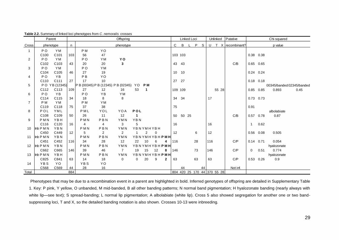
Phenotypes that may be due to a recombination event in a parent are highlighted in bold. Inferred genotypes of offspring are detailed in Supplementary Table
1. Key: P pink, Y yellow, O unbanded, M mid-banded, B all other banding patterns; N normal band pigmentation; H hyalozonate banding (nearly always with
white lip—see text); S spread-banding; L normal lip pigmentation; A albolabiate (white lip). Cross 5 also showed segregation for another one or two band-
suppressing loci, T and X, so the detailed banding notation is also shown. Crosses 10-13 were inbreeding.
Table 2.2. Summary of linked loci phenotypes from C. nemoralis crosses
Putative
Cross n C B L P S U T X recombinant?
1 P O Y M P M Y O
C100 C101 103 56 47 103 103 0.38 0.38
2 P O Y M P O Y M Y O
C102 C103 43 20 20 3 43 43 C/B 0.65 0.65
3 P O Y M P O Y M
C104 C105 46 27 19 10 10 0.24 0.24
4 P O Y B P B Y O
C110 C111 27 17 10 27 27 0.18 0.18
5 P O Y B (12345) P B (00345) P B (12345) P B (02345) Y O P M 00345/banded 02345/banded
C112 C113 109 27 12 16 53 1 109 109 55 28 0.85 0.85 0.893 0.45
6 P O Y B P O Y B Y M
C114 C115 34 18 8 8 34 34 17 0.73 0.73
7 P M Y M P M Y M
C119 C118 75 37 38 75 0.91
8 P O L Y M L P M L Y O L Y O A P O L albolabiate
C108 C109 50 26 11 12 1 50 50 25 C/B 0.57 0.78 0.87
9 P M N Y B H P M N P B N Y M N Y B N
C116 C120 16 4 4 3 5 16 16 1 0.62
10 Inb P M N Y B N P M N P B N Y M N Y B N Y M H Y B H
C450 C449 12 5 2 2 1 2 0 12 6 12 0.56 0.08 0.505
11 Inb P M N Y B N P M N P B N Y M N Y B N Y M H Y B H P M H
C451 C452 116 34 28 12 22 10 6 4 116 28 116 C/P 0.14 0.71 0.054
12 Inb P M N Y B N P M N P B N Y M N Y B N Y M H Y B H P M H hyalozonate
C662 C665 146 39 46 7 19 15 12 8 146 73 146 C/P 0 0.51 0.774
13 Inb P M N Y B H P M N P B N Y M N Y B N Y M H Y B H P M H hyalozonate
C825 C841 63 14 18 0 0 20 9 2 63 63 63 C/P 0.53 0.26 0.9
14 Y B S Y O Y B S Y O
C568 C569 44 28 16 44 44 Not inf.
Total 884 804 420 25 170 44 370 55 28
Chi-squared
phenotype phenotype p value
Parent Offspring Linked Loci Unlinked

30
2.2.2. DNA extraction, quantification and amplification
The DNA of progenitors and their progeny was extracted and genotyped by using RAD
markers. The goal was to create a base for future mapping of the supergene and the
possible identification of other shell trait genes close to or within the supergene.
Furthermore, we wished to identify individuals that show evidence of recombination,
ideally either close to a shell-character locus, or between loci within the supergene.
Past research achieved isolation of flanking RAD-seq markers near the supergene
(Richards et al., 2013). Those markers were used with the objective to accept or reject
possible recombinant phenotypes within the supergene features. To do so, frozen
snail tissue was used to extract genomic DNA as explained (Richards et al., 2013).
Two extraction methods were used. Foot tissue was chosen as it is known as
a good resource of high molecular weight DNA. Foot samples were cut in tiny slices
and added into 15ml Falcon tubes. 5ml of extraction solution (3% CTAB, 100mM Tris‐
HCl, pH 7.5, 25mM EDTA, pH 8, 2M NaCl) and 60µl Proteinase K (0.2 mg/mL) was
inserted. The culture was incubated at 60-62 oC inverting gently occasionally
overnight. Next day, RNAase A (80 μg/mL) was add to each tube and was incubated
for 1 hour to remove RNA. The mixture was cooled down at room temperature. Upon
lysis, a chloroform extraction was conducted, then three volumes of CTAB dilution
solution was inserted (1% CTAB, 50 mm Tris‐HCl, pH 7.5, 10mM EDTA, pH 8).
Samples were combined until a precipitation emerged, then the supernatant was
removed. The pellet was washed twice in 0.4M NaCl in TE (0.4M NaCl, 10 mM Tris‐
HCl, pH 7.5, 1 mm EDTA, pH 8), re-dissolved in 1.42M NaCl in TE (1.42M NaCl, 10mM
Tris‐HCl, pH 7.5, 1 mM EDTA, pH 8), then ethanol was used to precipitate DNA,
followed by centrifugation and drying. Latterly, a few samples were lysed in lysis buffer
(10 mM Tris, 0.1 M EDTA, 0.5% SDS), then extracted using the standard phenol-
chloroform protocol. Protocol changed due to the product availability and sample
conditions.
With the aim to flank the supergene, groups of samples from the key crosses
were genotyped by following personalized assays from the RAD-seq markers.
Therefore, two standard PCR methods were performed depending on the RAD-seq

31
marker. One option was the Amplitaq Gold polymerase (Invitrogen) that allows with
very high sensitivity or specific amplification of DNA targets. The PCR programme
applied for this polymerase was a single cycle of 95 °C for 10 min were used, followed
by 35 cycles of 95 °C for 30 s, 58 °C for 30 s, and 72 °C for 1 min. The other PCR
option was Clontech Advantage 2 PCR, which it is an extremely versatile polymerase
mix that has three times higher fidelity than other Taqs. This PCR method started with
an initial denaturation of 95 °C for 1 min, followed by 35 cycles of 95 °C for 15 s, 65
°C for 1 min, 68 °C for 1 min, and 72 °C for 1 min.
The genotyping and the particular primers used in each assays were based on
the prior characterised RAD-seq loci (Richards et al., 2013). These varied depending
on each cross. Primers applied were RAD06F 5’-GCCTATCCGTCATTGTTGGT-3’,
RAD06R 5’-GTCAAGGCTTGCTTCTTTGG-3’, RAD9F 5’-
TTTCTCGGAACGACGGAGT-3’, RAD9R 5’-GGTCTCGTCAATGGCACTTT-3’,
RAD11F 5′-AAGAAGCGTCCTTCTGGAAA-3’, RAD11R 5’-
CACCTTCCCCATTCTTCAAA-3’. Then, a restriction enzymatic digestion was
performed by 1-hour incubation usually at 37oC. Subsequently, the scoring of the
genotype were carry out in agarose electrophoresis gel. The details of the respective
of enzymes used with each assay and each cross are shown in the Supplementary
Table 2.3. Finally, the recombination rates were estimated by calculating the
recombination fraction estimation of the offspring (Ott, 1999).

32
2.3 Results
2.3.1. Segregation of Mendelian loci that determine shell phenotype
Shell colour, locus C, showed segregation in crosses 1–13 (Table 2.2; Supplementary
Table 2.1, 2.2, 2.3), only deviating significantly from expected Mendelian segregation
ratios in cross 12, with fewer yellow shells than expected.
Crosses 1–6 and 8 showed segregation for the band presence/absence locus,
B, with no deviations from expected Mendelian ratios.
Crosses 6 and 9–13 showed segregating variation for the mid-band phenotype,
coded by the unlinked U locus. The observed phenotype frequencies did not differ
from the expected frequencies.
Crosses 10 to 13 showed segregation for the pigmentation (hyalozonate; P)
locus, with no deviations from expected Mendelian ratios.
Cross 8 showed segregation for the putative lip colour locus, L. The offspring
phenotype frequencies would be consistent with single locus, assuming that L is part
of the supergene and treating lip colour phenotypes as either normal (N) or albolabiate
lip (A); there was no deviation from expected Mendelian ratios. Offspring in several of
the other crosses, especially 10–13, showed considerable and apparently continuous
variation in lip colour. We, therefore, tried to score the lip phenotype in the conventional
manner, having a phenotype as normal, pale, or albolabiate, and reconcile this with a
knowledge of the parental phenotypes and genotypes (parents in crosses 8 and 9).
No scheme that we devised fitted a simple Mendelian model. This fits with previous
studies (Cain Arthur James 1968; Cook, 2003). Unfortunately, it was not possible to
quantitatively measure the lip colour, as we have done for shell ground colour (Davison
et al., 2019a), because the coloured part of the lip was frequently too small and also
on a curved surface.

33
Cross 14 showed segregating variation in the spread band phenotype.
However, as one parent was homozygous for the dominant spread band allele SS, the
cross was non-informative for recombination with other supergene loci.
Finally, cross 5 showed segregating variation for the locus that suppresses the
first two bands, converting a five-banded snail (12345) to three-banded (00345). The
offspring phenotype frequencies would be consistent with single locus, with T345
dominant to T-, with both parents being heterozygote, except that this would require
both parents to have a T345 allele; apparently not possible because one of the parents
is 12345. As five of the offspring with suppressed bands have 02345 phenotype and
eleven a 0:345 (: = trace) phenotype, then the results are consistent with their being
two band-supressing loci, one that causes the 00345 phenotype and another that
causes the 02345/0:345 phenotype (see Supplementary Table 2.3 for inferred
genotypes).
2.3.2. Putative recombinants between colour, banding and lip and band
pigmentation loci.
Previously, the colour (P/Y) and banding (B/O) phenotype for six crosses (1, 4,
5, 6, 7, 8) and 398 offspring was reported, and the genotype of flanking RAD-seq loci
reported for cross 1 (Richards et al., 2013). In this new work, we raised a further 486
offspring from eight more crosses, and genotyped six further crosses using flanking
RAD-seq loci. The combined data set of parent and offspring phenotypes, alongside
inferred genotypes, is presented here together, summarised in Table 2.2, S2.1, S2.2,
and presented in full in Supplementary Table 2.3.
Offspring in several crosses (2, 8 and 10-13) produced snails with phenotypes
that could be explained by a recombination event within the supergene of the
heterozygous parent (Fig. 2.1).

34
Figure 2.1. Shells of offspring from crosses, including putative recombinant individuals, and one wild
collected individual. A) Normal yellow mid-band, b) yellow, trace of banding, c) yellow, no band. An
absence of banding suggests that individual 366 is a putative recombinant. D) normal pink mid-band,
showing evidence of white “highlighting” of pigmented band e pink, trace of banding, some highlighting
f) pink, no band, very faint mark where band would be. An absence of banding suggests that individual
536 is a putative recombinant. G) Normal pink mid-banded, showing evidence of white highlighting of
pigmented band h) pink, no band, white highlighting i) yellow, mid-band hyalozonate, j) yellow, banded
hyalozonate (02345) k) yellow, mid-band hyalozonate. An absence of dark pigment suggests that 822
is a putative recombinant; however, the shell has retained the white highlighting pigment. Hyalozonate
shells generally lack both dark and light pigment, see i) and j); this is not always easily visible, see k).
In a wild-collected pink hyalozonate, l) the lack of pigment is just visible on some whorls, and not at all
on some upper whorls, or from the inside.
35
Cross 2 produced three yellow unbanded snails (e.g., Fig. 2.1c), a phenotype
that might be produced by recombination between the colour (C) and banding (B) loci;
one of these individuals, a sub-adult with a damaged shell, has a very faint trace of a
band. A few other snails in the same cross have much-reduced banding (e.g., Fig.
2.1b).
Cross 8 produced a single pink unbanded snail, a phenotype that is also best
explained by recombination between the colour (C) and banding (B) loci (Fig. 2.1f).
Very few of the snails in this cross have reduced banding. This cross also segregated
for the lip pigmentation locus, L. As the recombinant snail has a pigmented lip (see
Fig. 2.1f, lip image), then this cross in theory informs upon the order of loci within the
supergene (but see below).
Cross 5 produced a single pink mid-banded snail. This phenotype is very
difficult to explain by recombination, based on the known genotypes (Supplementary
Table 2.3 and 2.4). As the pink colour of this snail is qualitatively different from the
other pink-banded snails in this cross, the best explanation is that it is a likely a
contaminant from another cross.
The remaining crosses produced offspring that suggest possible recombination
between the colour C and band pigmentation P loci. Crosses 11, 12 and 13 produced
several unbanded pink individuals, with pigmented lips (e.g., Fig. 2.1h). These were
initially scored as hyalozonate, because the mid-band was evident but not pigmented.
However, closer inspection revealed that the banding phenotype of these shells is not
the same as the yellow hyalozonate shells. Specifically, the unbanded pink individuals
retain the white highlighting pigment of a normal shell, but lack the dark pigment
(compare Fig. 2.1h with 2.1g). This difference is especially evident when viewed from
the underside: hyalozonate shells have cleared bands which are entirely lacking
pigment whereas the white pigment of ‘unbanded’ snails shows a silhouette (compare
Fig. 2.1h with 2.1i, j). Not all of the hyalozonate shells show such a clear pattern (e.g.,
Fig. 2.1k). For comparison, in a wild collected pink hyalozonate, the cleared bands are
only evident on the upper whorls (Fig. 2.1l); in another shell they are not evident at all.
36
2.3.3. Genotyping of offspring using RAD-seq derived loci
Individual offspring from crosses 1, 2, 8, 9, 10, 11, 12, and 13 were genotyped using
custom assays derived from RAD-seq loci that flank either side of the supergene,
using RAD06/RAD11 on one side and RAD09 on the other side (Table 3;
Supplementary Table 2.3). Unfortunately, the RAD-seq loci in cross 5 lacked
polymorphism so no assay was possible. To confirm or refute individual recombination
events, we inspected the genotype of the putative recombinant offspring. In theory,
individuals for which we have inferred recombination within the supergene should also
show recombination by one of the RAD-markers.
None of the three individuals from cross 2 showed evidence of recombination
from the flanking loci RAD11 and RAD09. Similarly, the single individual in cross 8 did
not show evidence of recombination for the same RAD-seq loci. All eight putative
recombinants in cross 12 and all three in cross 13 showed no evidence of
recombination using RAD06 and RAD09; in cross 11, three individuals did not show
evidence of recombination, with one single individual (804) showing recombination
between RAD06 and the supergene and apparent recombination between the colour
and pigmentation loci (C/P). If this were correct then it would inform the order of loci
within the supergene. However, the phenotype of this snail is exactly the same as the
other refuted recombinants (Fig. 2.1h). It is most likely not a hyalozonate, and
therefore a coincidence that it also shows recombination between RAD06 and the
supergene.
Thus, overall, while there is incomplete evidence in some cases, we were not
able to confidently confirm any recombination events within the supergene. This puts
the point estimate on recombination between C and B at 0/376 (<0.27%), between C
and P at 0/170 (<0.60%) and between C and L at 0/25 (<4%). Therefore, the upper
confidence limit for the mean rate of recombination, assuming that the probability of
observing zero recombination events is 5%, is 0.80% for C/B, 1.76% for C/P, and
12.0% for C/L. Of course, as there are no recombination events, then this work does
not inform the order of loci within the supergene; the higher upper limits for C/P and
C/L are due to smaller sample sizes.

37
RAD06 and RAD11 flank one side of the colour and banding loci of the supergene; RAD09 flanks the other side. Full genotypes are in Supplementary Table
2.3.
Table 2.3. Summary of RAD-seq marker genotyping, putative number of supergene recombinants and actual number.
RAD11 RAD06 RAD09 RAD11 RAD06 RAD09
1 C100 C101 P O Y M 101 102 102 1 10 1 0 0
2 C102 C103 P O Y M 38 43 0 2 3 0
8 C108 C109 P O L Y M L 44 50 2 1 1 0
9 C116 C120 P M N Y B H 16 16 2 0 0 0
10 C450 C449 P M N Y B N 12 12 2 1 0 0
11 C451 C452 P M N Y B N 103 104 4 2 4 1?
12 C662 C665 P M N Y B N 127 132 3 6 8 0
13 C825 C841 P M N Y B H 44 49 4 1 3 0
Genotypes Putative supergene
recombinants
Actual supergene
recombinants
Cross Recombinants between
supergene and:Snails and phenotypes

38
2.4. Discussion
For future mapping and the precise identification of the supergene, it would be useful
to identify individuals that are known to have a recombination break-point close to, or
within the supergene. In this study, we initially identified four putative recombination
events between the colour and banding loci (C/B) and fourteen putative recombination
events between the colour and pigmentation loci (C/P). This is as expected because
historic studies have indicated that C/B are more tightly linked than C/P. We also used
genotyping of RAD-seq loci that flank the supergene in several of the crosses to reveal
individuals that show recombination between a linked RAD-seq marker and the
supergene. These RAD-seq markers may, therefore, be used for future recombination
break-point mapping. However, the same RAD-seq genotyping did not find any
evidence of recombination thereby refuting the putative recombinants detected above.
This is also supported by a close analysis of the phenotype of the shells, including
variable penetrance of the mid-band phenotype (Fig. 2.1; crosses 2, 8, 11–13) and a
comparison of true hyalozonate shells against shells that partially lack pigmentation
(Fig. 2.1; crosses 8, 11–13).
Therefore, in contrast to previous studies that have reported rates of
recombination between C/B of 0–2% and between C/B and the pigmentation locus, P,
of 3–15%, which were not supported by genetic data. We found zero recombinants,
putting upper limits on the rate of recombination at 0.8 and 1.8%, respectively. This
does not mean that previous inferences of recombination within the supergene were
incorrect. However, as the ‘recombinants’ in this study are better explained by other
means, then we would suggest that there is an absence of modern-day evidence for
recombination within the C. nemoralis supergene. The structure of the supergene may
not be as has previously been supposed.
2.4.1. Incomplete penetrance and epistasis
Four individuals in crosses 2 and 8 were initially identified as putative recombinants,
because they lacked the mid-band, or had only very faint traces of a band. If these
snails had been true recombinant individuals then they would most likely be

39
homozygous for colour and heterozygous for banding (genotype B0Bb). Incomplete
penetrance of the dominant B0 allele could mean that some individuals show evidence
of banding (e.g., Fig. 2.1b, e). Instead, the genotyping shows that these individuals
are not recombinant, and so must be genetically homozygous for colour and banding
(BbBb). Therefore, the best explanation for their phenotype is that other loci are
interacting epistatically to prevent full penetrance of homozygous banding alleles.
Similarly, up to fourteen individuals were identified that were putative
recombinants between the colour and pigmentation loci. If they had been true
recombinants, then they would most likely be heterozygous for colour and
homozygous for pigmentation (CPCYPHPH). However, close analysis of the phenotype
and the genotyping together show that they are not recombinants and therefore, more
likely they were heterozygous for both colour and pigmentation (CPCYPNPH). These
same snails are homozygous for the banding locus (BbBb), but segregate for mid-band
phenotype (U3U-, U-U-); the putative recombinants were always mid-banded (U3U-),
rather than fully banded (U-U-). The same explanation may apply, as above. Other loci
sometimes interact to prevent full penetrance of the mid-banded phenotype.
The observation that the absence of a mid-band does not always have a simple
genetic basis may shed some light on previous findings. For example, both Fisher et
al. (1934) and Cain et al. (1960) reported individual crosses that showed elevated
rates of recombination between the C/B loci.
Cain et al. (1960) reported two crosses derived from the same mother that
showed seven colour/banding recombinants in 43 snails, for which six were pink mid-
banded snails. The expectation is that putative recombinants would have been
homozygous for the banding locus (CPCYBbBb) and non-recombinants heterozygous
(CPCYB0Bb). However, if the six snails were not actually recombinants, then incomplete
dominance of the band-suppressing allele (B0), or else epistatic interactions with other
loci, may be an alternative explanation.
Similarly, Fisher and Diver (1934) described unexpectedly high recombination
(20%) between colour and banding in one cross. Unfortunately, they did not report
whether the snails used were mid-banded or not. However, in their specific case, doubt

40
has been raised as to whether the individuals used were virgins before paired together
(Cain et al., 1960; Ford, 1971; Lamotte, 1954). In researching this work, we were
fortunate to find copies of letters between Fisher and Diver in the archive of Bryan
Clarke (Supplementary Material). In letters from April/May 1934 that describe the
preparation of the correspondence that was published in Nature in June 1934, there
is clear admission that the snails used in the crosses were adult and not virgin. The
authors partly acknowledge that this may be a problem. Referring to possible previous
matings (“experience”), Fisher writes that "on fairly strong ground, which is not
weakened by previous experience, but is not absolutely critical". Our interpretation of
the text is that Fisher acknowledges that the snails may have previously mated, but
discounts this as being a problem, because the offspring ratios approximate to that
expected with limited recombination. There are therefore perhaps two errors, which
together invalidate the conclusions of the published work.
Epistasis could also explain other earlier data on recombination between the
C/B loci and the pigmentation locus. For example, in our study, we initially scored
some pink individuals as hyalozonate, even though they had a lightly pigmented lip,
only later realising our error. Other authors may have made the same mistake.
Unfortunately, it is difficult to be certain from the previous literature whether pink
hyalozonate recombinant individuals had an unpigmented lip, though if this was not
the case then it might have been explicitly noted (e.g. p404 in Cook, 1967). However,
just as it is hypothesised that epistasis makes brown shelled individuals less likely to
be banded, then it is reasonable to suppose that epistasis might mean that pink
hyalozonates more rarely have a wholly unpigmented lip.
Evidently, further crosses are required, especially with respect to the other
major loci, especially pigmentation, spread band and punctate loci in the supergene,
and the various band-modifying genes. It is possible that some of these phenotypes,
especially those for band-modification (Wolda, 1969), are under multi-factorial control
and/or dependent upon genetic background. A further general consideration is that the
genetics may differ depending upon the location of origin of the snails. In our study,
the snails are derived from the UK, Ireland or Spain, and hybrids between them. As a
previous mitochondrial DNA study has shown that the Cepaea snails in the West of
Ireland are at least partly derived from snails from the Pyrenees, and genetically

41
divergent from those of the UK, then perhaps location should be more properly
considered (Richards et al., 2013).
2.4.2. Future progress
Overall, this research proposes an alternative explanation to the putative non-
recombinant phenotypes found. However, future steps are necessary to confirm that
these results are due to incomplete penetrance or epistasis. Perhaps, an epistasis
mapping method using, for example, QTL mapping studies to determine the
expression of the genes involved may be a clever next step to verify this explanation.
Moreover, this work also provides a resource for fine mapping of the supergene, and
the other major shell phenotype loci. On the one hand, we have shown that
phenocopies may be a problem in using the shell phenotype alone to detect
recombination events within the supergene. On the other hand, the genotyping
methods that we have introduced enable a means to avoid this problem.
Jones et al. (1977) (in)famously questioned whether understanding
polymorphism in Cepaea is “a problem with too many solutions?” The intention of that
work was to emphasise the perfect case study provided by Cepaea. We hope that
these crosses may soon be used with new long-read DNA sequencing methods to
assemble the C. nemoralis genome and to identify the supergene. Perhaps soon,
polymorphism in Cepaea may instead be considered “a solution to many problems.
2.5. Acknowledgements
This work was supported by the University of Nottingham; the Biotechnology and
Biological Sciences Research Council [grant number BB/M008770/1], via a
studentship to Daniel Ramos Gonzalez; and the Dept. of Education, Universities and
Research of the Basque Government [grant numbers PRE_2015_2_0191,
EP_2015_1_33], via a visiting fellowship awarded to Amaia Caro Aramendia. Thanks
to both Sheila Keeble and Julie Rodgers for help with the care of snails, and to
Laurence Cook as well as three anonymous referees for comments on the manuscript,
and to Anne Clarke and the University of Nottingham for access to the archive of
Professor Bryan Clarke.

42
Chapter 3:
Exploring the divergence of genomic variation and
geographical structure in Cepaea nemoralis.
Abstract
Colour variation is considered a driver in the adaptation to the environments in many
species. In Cepaea nemoralis, it is well-known different shell ground colour are under
various forms of selection and in to different environments. To what extent does this
selection impact on the wider genome and across different environments? To begin to
understand these factors, double digest restriction-site associated DNA (ddRADseq)
was conducted to comprehend hidden patterns of its genomic variation, diversity and
structure. Surprisingly, even though there was an association between genomic
variation and the geographical distribution, colour variation was unrelated. The
genomic areas leading the geographic variation were examined and several candidate
sequences under selection were found. However, these candidates need further
analyses to confirm which their involvement in the environmental adaptation. In
addition, the phylogenomic structure of West European populations of C. nemoralis
was inferred leading to an interpretation of how Pyrenean snails colonised Europe
after the Pleistocene. The results may launch new roads of research into the
evolutionary and genomic mechanisms that have led the geographical genomic
variation and the supergene variation.

43
3.1. Introduction
Over the past century, the study of animal colour has been key in providing evidence
for some of the central tenets of biology, especially with respect to genetics and
evolution. For example, early work on the inheritance of colour traits contributed to an
initial understanding of Mendelian genetics (Staples‐Browne, 1908; Wheldale, 1907).
Subsequent studies on the distribution and predation of colour morphs shaped our
understanding of how natural selection may operate in wild populations, with perhaps
some of the most important insights coming from moths and snails (Cain et al., 1950;
Cook, 2003). In the 21st century, next-generation DNA sequencing technologies, such
as genotyping-by-sequencing, have been used to identify the underlying genes that
determine variation in colour morphs within species, and their evolutionary history
(Wellenreuther et al., 2014). These same methods have also enabled the sub-
discipline of phylogeography to move away from the use one or a few molecular
markers to a genomic overview, usually involving thousands of genetic markers
(Dussex et al., 2020; Kotlík et al., 2018; Lucena‐Perez et al., 2020). Such studies have
revealed how connectivity between populations – or lack of – shapes the genetic
structure of species, and critically, how regions of the genome respond differently
depending upon the nature of selection and the genetic architecture of a particular
colour trait (e.g. Pardo-Diaz et al., 2012; Poelstra et al., 2014).
Historically, some of the most important animals in studying colour
polymorphism have been the Cepaea species, C. nemoralis and C. hortensis. This is
partly because they are relatively easy to collect, but also because the different colour
and banding morphs (Figure 1.1) show straightforward inheritance (Cook, 2017; Jones
et al., 1977) – the shell polymorphism is controlled by a series of nine or more loci, of
which five make a single ‘supergene’ containing tightly linked colour, banding and
other loci. In these two species, we now have some understanding of the pigments
and shell proteome (Affenzeller et al., 2020; Mann et al., 2014; Williams, 2017) and
have begun to use new genomic methods to identify the genes involved (Kerkvliet et
al., 2017; Richards et al., 2013).

44
However, while ongoing studies on snails in general continue to provide
evidence for the relative role of various forms of natural selection and random drift in
promoting and maintaining variation, as a group they are generally poorly represented
in phylogeographic or population genomic studies. For example, most studies of
phylogeography and/or population structure in terrestrial snails have been limited to
using just one or a few genes, with a few notable exceptions (Chueca, 2020), and
better representation for aquatic snails, especially Littorina (Hirano et al., 2019; Miura
et al., 2020; Westram et al., 2018). This is a problem because if the ultimate aim is to
understand the role of natural selection in promoting and maintaining colour
polymorphism, then we require an understanding of the history of populations in
general, and more precisely, a gene-by-gene account of how historical contingencies,
including drift, and selection have impacted upon the genome.
One issue for Cepaea is that Steve Jones and colleagues (1977) questioned
whether understanding the polymorphism is “a problem with too many solutions?”,
which led to difficulties arguing the case for these snails as a study organism. Actually,
the misunderstood intention of that work was to emphasise the perfect case study
provided by Cepaea. Simple explanations for phenotypic variation, including colour,
are likely an exception, so they were making the point that it is important to study
organisms for which polymorphism may be explained by a variety of processes,
precisely because they are more realistic. Given that present-day genomic
technologies should allow us to uncover the relative contributions of each of these
processes in making contemporary diversity, this point is perhaps just as prescient
now.
Unfortunately, a second general issue is that is DNA from snails is sometimes
difficult to work with (Adema, 2021), and snails in general have large and repetitive
genomes, which are difficult to assemble. Advances in the understanding of the colour
polymorphisms of snails have therefore tended to lag behind other species, especially
invertebrates with relatively small genomes (Davison et al., 2020).
Historically, studies on the colour polymorphism of Cepaea have mainly been
based on comparisons of morph frequencies between different habitats. More
recently, data from much of the 20th century collections were digitised by the

45
“Evolution Megalab” project (Silvertown et al., 2011), so that comparisons can be
made across the generations. Some of these comparative studies found that discrete
colour variation were associated with geographic variables such as latitude, longitude,
altitude and even by regions. For example, in larger studies yellow snails were
commonly found at mid-latitudes (Jones et al., 1977; Silvertown et al., 2011).
Moreover, in local surveys discrete colour patterns were mostly associated by the
regions. For instance in the Pyrenees, each valley showed sharp frequency
discontinuities in colour variation due to different selective pressures such as climatic
or predation (Arnold, 1968; Cameron et al., 1973; Jones et al., 1975).
There have also been some genetic studies, first using allozymes and latterly
mitochondrial DNA and microsatellites (but only at a local geographic scale; Davison
& Clarke, 2000). Of most relevance here, Ochman et al. (1983) showed using
allozymes that the Pyrenees contains three deeply differentiated sets of populations,
or “molecular area effects”, for which the geographic patterns did not correlate with the
shell ground colour and banding frequencies. Latterly, we surveyed much of Europe
using a mitochondrial marker (Grindon et al., 2013a). As with Ochman’s study, high
differentiation was found within the Pyrenees and the North of Spain. However, the
main finding was that of the seven deep mitochondrial lineages, one was found only
in Ireland and in a region of the Eastern Pyrenees in southwest Europe. As the oldest
C. nemoralis fossils in Ireland date to about 8,000 years ago, around the time that
modern humans began to inhabit the island after the glaciations, the suggestion was
that ancient humans might have carried the edible snails with them as they moved
between the Mediterranean and the Atlantic, following the Garonne river (Grindon et
al., 2013a).
In this study, we take advantage of a first draft genome sequence (Saenko et
al., 2020) and restriction-site associated DNA sequencing methods (ddRAD) to
understand the phylogeographic and population genomic structure of C. nemoralis.
Using samples from across Europe, the specific aim is to understand the post-glacial
history of the species, at both the level of the whole genome, and more specifically,
with respect to the supergene that is responsible for a large part of the colour and
banding polymorphism. The ultimate aim is to provide context for subsequent studies
on the evolutionary origins of the supergene, and the relative roles that natural

46
selection and drift may play in the establishment and loss of colour polymorphism in
local populations.

47
3.2. Materials and Methods
3.2.1. Dataset collection
In previous work, we collected C. nemoralis from across Europe, euthanising snails by
freezing at −80°C upon arrival at the University of Nottingham. In this study, we
strategically sampled from this prior collection, including individuals from Germany,
Belgium, France, Hungary, Denmark, Spain, UK and Ireland, as well as a 2017/2018
collection from three valleys in the Pyrenees, Valle de Vielha, Valle de Jueu and Valle
Noguera Ribagorzana. Individuals were selected to ensure a wide geographic spread,
and to include representatives of most of the major mitochondrial lineages reported in
a prior study (Figure 3.1, Table 3.1; Grindon et al., 2013a).
Figure 3.1. European map shows the geographical coordinate points of the sampling sites collected by
Grindon and Davison (2013). Each population (red dots) is labelled by its abbreviation. In addition, an
Eastern Pyrenean map is added. Three valleys from the Central Pyrenees were sampled in 2017;
Vielha, Jueu, N. Ribagorzana. The other three; Commitges, Segre and Benasque were acquired from
Grindon and Davison (2013).

48
Location ID Grindon ID Abbreviation Latitude Longitude
Mitochondrial
Haplotype Colour Banding
Belgium / Moortsele 48 Ooscn2 Moo 50.9588 3.7798 A27 Yellow 12345
Denmark / Aalborg 46 Aal2cn5 Aal 57.0518 9.8728 A51 Yellow 12345
47 Aal2cn7 Aal 57.0518 9.8728 A22 Pink 12345
England / Cornwall 26 Coascn3 Cor 50.2535 -5.0404 A87 Yellow 00000
66 Coascn5 Cor 50.2535 -5.0404 A87 Yellow 00000
France / Pont L'Abbe 28 Abbecn1 Abb 47.884 -4.1826 A58 Pink 00300
29 Abbecn3 Abb 47.884 -4.1826 A85 Yellow 00300
Germany / Jessern 49 Jesscn1 Jes 52.0167 14.1833 A11 Brown 00000
51 Jesscn9 Jes 52.0167 14.1833 A40 Pink 00300
Scotland / Mull Isle 27 Muulcn4 Mul 56.5785 -6.2775 A47 Pink 12345
England / Malham 53 Malcn3 Mal 54.0618 -2.1467 B16 Yellow 12345
54 Malcn5 Mal 54.0618 -2.1467 B8 Yellow 00000
England / Saltmill 52 Saltcn9 Sal 54.4893 -3.5895 B3 Pink 00300
France / La Roche 31 Berncn2 Roc 47.5118 -2.2857 B23 Brown 12345
Ireland / Dublin-Ranelagh 38 Dublincn4 Dub 53.3185 -6.2514 C15 Pink 12345
39 Dublincn2 Dub 53.3185 -6.2514 C15 Yellow 00345
Ireland / Lisdoonvarna 36 Liscn1 Lis 53.0263 -9.2902 B27 Yellow 12345
37 Liscn2 Lis 53.0263 -9.2902 C8 Yellow 12345
Spain / Benasque 61 Bencn3 Ben 42.5994 0.527 C18 Yellow 12345
62 Bencn1 Ben 42.5994 0.527 C17 Pink 00000
Spain / Commitges 63 Romancn5 Com 43.028 0.7223 C57 Brown 00345
64 Romancn7 Com 43.028 0.7223 C56 Pink 00000
Spain / Jueu 34 - Jue 42.6779 0.7055 - Yellow 00000
56 - Jue 42.6779 0.7055 - Pink 00000
Spain / Ribagorzana 57 - Rib 42.4792 0.714 - Yellow 00000
58 - Rib 42.4792 0.714 - Pink 00000
Table 3.1. Summary showing the locations and phenotypes of the samples used in this study, including mitochondrial
haplotype from Grindon and Davison (2013).

49
Spain / Segre 59 Serge2cn1 Seg 42.3598 1.4796 C1 Yellow 12345
Spain / Vielha 32 - Vie 42.6905 0.8742 - Yellow 12345
33 - Vie 42.6905 0.8742 - Pink 00000
Belgium / Leuven 40 Kesscn5 Leu 50.8835 4.7225 D39 Yellow 00300
45 Kesscn8 Leu 50.8835 4.7225 D8 Yellow 00000
Germany / Mecklenburg 50 Robcn2 Mec 53.5817 12.985 D33 Pink 00300
Spain / Santander 60 Santacn8 San 43.4144 -3.7413 F24 Yellow 00000
65 Santacn9 San 43.4144 -3.7413 F25 Pink 00000
30 Playacn9 San 43.487067 -3.792683 D49 Yellow 00000
35 Playacn10 San 43.487067 -3.792683 D47 Yellow 00000
55 Playacn7 San 43.487067 -3.792683 F24 Yellow 00000
Spain / Roncesvalles 41 Roncscn3 Ron 43.0093 -1.3191 F41 Pink 12345
Hungary / Budapest 42 Hungcn4 Bud 47.4258 19.4483 G11 Yellow 12345
43 Hungcn5 Bud 47.4258 19.4483 G13 Yellow 00300
44 Hungcn1a Bud 47.4258 19.4483 G12 Yellow 00300

50
3.2.2. Genomic methods
High molecular weight genomic DNA was extracted from frozen snail tissue, similarly
to the method described previously in Chapter 2.2 section (Gonzalez et al., 2019;
Richards et al., 2013), using foot because it is a good source of high molecular weight
DNA. In brief, slices of snail tissue were incubated at 65 °C in lysis buffer (10mM Tris,
0.1M EDTA, 0.5% SDS), with proteinase K (0.2 mg/mL), with occasional inversion.
RNAase A (80 μg/mL) was added, and then each tube was incubated for one more
hour to remove RNA. The mixture was cooled to room temperature, and then extracted
using the standard phenol/chloroform/iso-amyl ethanol (25:24:1) method, with ethanol
precipitation. DNA quality was visually verified by agarose gel electrophoresis, and
then quantified and further checked using a spectrophotometer (Nanodrop 2000c) and
a fluorometer (Qubit 2.0 Fluorometer). RAD-seq libraries were generated by
SNPsaurus (https://www.snpsaurus.com/), using the method of Russello et al. (2015)
and 75 ng of input DNA. One lane of a HiSeq4000 (University of Oregon) was used to
generate 150 bp sequence reads, which were then demultiplexed and stored as fastq
files.
3.2.3. Sequence analysis and datasets
FastQC software was used to check the quality of the reads, then adapters removed
using Trimmomatic (Bolger et al., 2014) with the following settings; ILLUMINACLIP:
trimmomatic/adapters/NexteraPE-PE.fa 2:30:10
(prefixNX/1:AGATGTGTATAAGAGACAG, prefixNX/2:AGATGTGTATA AGAGACAG,
trans1:TCGTCGGCAGCGTCAGATGTGTATAAGAGACAG,
trans1_rc:CTGTCTCTTATACACATCTGACGCTGCCGACGA,
trans2:GTCTCGTGGGCTCGGAGATGTGTATAAGAGACAG,
trans2_rc:CTGTCTCTTATACACATCTCCGAGCCCACGAGAC), and the
trimmomatic specific parameters; LEADING:5, TRAILING:5, SLIDINGWINDOW:5:10
and MINLEN:50 – 150. Files were then checked again using FastQC. The trimmed
fastq files were aligned to the C. nemoralis draft genome (~3.5Gb, Saenko et al., 2020)
using Burrows-Wheeler Alignment Tool (Roodi et al., 2019). Bcftools v1.10 (Danecek
et al., 2017) was then used to transform the sam output files to bam files, and then
Bam tools was then used to call variants and genotypes (Li, 2011). Vcftools was used

51
to extract bi-allelic loci, while only retaining those with less than 25% missing data, a
mean sequencing depth greater than 0.25 to a maximum of 25 reads, minimum quality
score of 20 and minor allele frequency (MAF) of 0.1 (Danecek et al., 2011). Finally,
allelic balance at heterozygotes test was used to detect contamination (Supporting
information).
Approaching the challenge to understand the genetic basis of the colour and
banding polymorphism in C. nemoralis, a set of 60 contigs from the draft genome were
identified to be tightly linked to the supergene that determines the colour and banding
of the shell. Contigs containing the supergene (~2.9 Mb) were found by Pool-seq
technique using colour variation (Saenko et al., 2020), and verified by finding within
them the flanking RAD-seq markers of the supergene (Richards et al., 2013). Two
different datasets were, therefore, generated from the filtered bi-allelic loci: 1) the
whole-genome RAD-seq dataset (hereafter “whole-genome”) 2) the subset of RAD-
seq loci that are putatively linked to the supergene (“supergene-linked”).
3.2.4. Analysis of genomic variation
To understand the broad phylogenomic relationship between individuals, a principal
component analysis (PCA) was performed. The filtered variant calling file was first
pruned using a linkage genotyping analysis in plink v1.9 (Purcell et al., 2007), then
linkage-pruned sites were used to generate eigenvalues and vectors. The PCA output
was plotted in R version 3.4.1 (2017-06-30) using the tidyverse v1.3.0 package. To
identify clusters within the genomic data, Gaussian finite mixture modelling was
undertaken using Mclust 5.4.6 (Scrucca et al., 2016), assuming 1 to 20 possible
clusters from the PCA results. The best fitting model was, then, determined by the
highest Bayesian Information Criteria (BIC), with significant differences established by
using a bootstrap likelihood ratio test, assuming varying orientations and homogeneity
of variance.
To understand the distribution of genomic variation by geography, pairwise
values of Weir & Cockerham’s Fst were estimated using Vcftools (Li, 2011). Genome-
wide Fst was used directly by plotting against geographic distance, or transformed into
a dissimilarity matrix, and again plotted against geographic distance. Geographic

52
distances were calculated in miles using the great circle formula in McSpatial 2.0
package in R (McMillen et al., 2013). Significance was tested using a Mantel test
based on Spearman’s rank correlation and 9999 permutations, using the vegan 2.5-6
community ecology package in R (Jari Oksanen et al., 2018). Then, to understand
how individual genome contigs shape the overall geographic variation, the same
analyses were carried out on each of the individual contigs, again testing significance
using a Mantel test.
Thus, to identify the possible RAD genomic regions under selection, the mean
of Fst pairwise estimation in each contig were calculated and Mantel statistic test were
executed as previously mentioned. The estimation of higher or lower genetic
differentiation than the expected under neutrality were evaluated by a simple
histogram of the Fst (Akey et al., 2002; Narum et al., 2011). Subsequently, the outliers
were determined using quantile range outliers statistic set at 97%. Finally, each
sequence selected was aligned and compared with the Genbank dataset looking for
homology with already described genes (Korf et al., 2003).
The whole-genome RAD-seq data was used to generate an unrooted
phylogeny, using randomized axelerated maximum likelihood (raxml) v8.2.9 with the
GTRGAMMA model and 100 bootstrap replicates (Stamatakis, 2014). An admixture
test was performed to group and cluster allocations for each individual and to estimate
the C. nemoralis ancestry (Alexander et al., 2011), computing the fivefold cross-
validation error to determinate the best number of clusters (K). Finally, D statistics
were calculated to identify evidence of introgression among targeted C. nemoralis
populations over Europe using Admixtools version 6.0 (Patterson et al., 2012) and
Admixr version 0.7.1 (Petr et al., 2019). To test robustness of the D statistics, different
populations were used as outgroup. In addition, the significance of the D statistics test
was evaluated using block jackknife and the Z-score.

53
3.3. Results
RAD-seq libraries were prepared from 41 snails and 22 locations across Europe.
(Table 3.1). A contamination and genotyping quality test were performed and two
samples were discarded due to a low number of reads (S57 and S58 both from
Ribagorzana valley in Spain; Supplementary material and Table S3.1). 39 individuals
were put through to the main analysis. An average of 95% of reads mapping to the
reference genome (Table S3.1). After filtering, the whole-genome dataset was
reduced to 8689 bi-allelic loci contained on 2323 genome contigs (out of 28,538 in the
reference), with a mean of 3.74 SNPs per contig (Figure S3.1). There was a correlation
between contig length and number of SNPs (r = 0.11, p < 0.001; Figure S3.2). Of the
60 contigs that are putatively linked to the supergene, 27 were represented in the
RAD-seq data, but only 7 had variants in the final dataset (Table S3.2). The
supergene-linked dataset was, thus, 31 bi-allellic SNPs found on 7 contigs.
3.3.1. West European phylogenomics of C. nemoralis
A principal components analysis of the whole-genome data showed that individuals of
C. nemoralis broadly cluster according to geography (Figure 3.2a)-c); PC1, PC2, and
PC3 together explained 37% of the variance; Figure S3.3). Gaussian finite mixture
modelling returned ten clusters as the best-fitting model (EII, spherical, equal volume;
BIC 349.2 and ICL 349.2; p < 0.001 compared with 2nd best model).

54
Figure 3.2. Relationship between individual Cepaea nemoralis snails across Europe based on 8689
biallelic loci using the whole-genome dataset. Figures are coloured according to the clusters defined by
Gaussian finite mixture modelling. a), b), c) First three axes of a principal component analysis of the
whole-genome data. d) Admixture analysis (K = 2), excluding the divergent individuals from Hungary
(Budapest), North Spain (Santander) and West Pyrenees (Roncesvalles). Each vertical bar represents
an individual, with the proportion of each colour representing the inferred ancestry e). Unrooted Raxml
phylogeny, showing bootstrap support. Region abbreviations are shown in table 3.1.

55
The principal component analysis showed that the Hungarian (Budapest, n =3)
samples and the North-West Iberian samples (Santander, n = 5; Roncesvalles, n = 1)
were different from the other samples, and also each other. This is because PC1
separated the Hungarian samples and North-West Iberian samples from the rest of
European populations (Figure 3.2a; PC1 = 15%), with PC3 separating the Hungarian
samples from the North-West Iberian samples, with the others somewhat intermediate
(Figure 3.2c; PC3 = 10%). PC2 separated the populations found in the central
Pyrenees (Vielha, Jueu & Benasque, n = 6; Commitges, n = 2; Segre, n = 1) from
samples found in central Europe and the UK (Figure 3.2b; PC2 = 12%), with samples
from Ireland (Dublin, n = 2; Lisdoonvarna, n = 2) and the West of France (Roche, n =
1) closest to the Central Pyrenean samples.
An unrooted phylogeny based on the whole-genome data corroborated the
principal components analysis, in recovering a North-West Iberian group, a Hungarian
group, a central European group (French, German, Danish and British) and a central
Pyrenean group, with the Irish populations closest to the latter (Figure 3.2e). Admixture
analyses using the whole-genome data were, then, used to understand prior gene flow
between the central European, Pyrenean and Irish populations. North-West Iberian
and Hungarian individuals were removed from the admixture analysis due to the lack
of shared ancestry. Admixture K =1 (0.91), 2 (1.00) were most strongly supported as
the best cluster values according to the cross-validation error test (Figure S3.4). For
K =2, individuals from the west of Ireland show mixed ancestry between the central
Pyrenees and Europe. Dublin, Roc and Mul also showed mixed ancestry. Finally, D-
statistical analysis using the whole-genome data were used to corroborate the
admixture analyses (Table 3.2). Firstly, the comparison between the European
populations (British, French, German and Danish) and Eastern Pyrenean did not
illustrate significant introgression. These results illustrated that both populations had
similar genetic introgression. However, significant introgression was shown when
comparing the above-mentioned populations to the Iberian populations (Table 3.2, 3
< Z-score < -3). According to D-statistic La Roche and the Irish populations are
significantly (Table 3.2, 3 < Z-score < -3) admixed between the Eastern Pyrenean and
European populations (British and Danish).

56
Population W Population X Population Y Population Z D-statistic std-error Z-score BABA ABBA SNP's
Lisdoonvarna:
Cornwall Lisdoonvarna Vielha Budapest -0.09 0.04 -2.32 178 215 3447
Malham Lisdoonvarna Jueu Budapest 0.01 0.03 0.21 278 275 5074
Aalborg Lisdoonvarna Benasque Budapest -0.07 0.05 -1.44 133 152 2708
Cornwall Lisdoonvarna Jueu Budapest 0.00 0.04 -0.08 186 187 3684
Malham Lisdoonvarna Benasque Budapest -0.06 0.04 -1.50 155 177 3228
Aalborg Lisdoonvarna Vielha Budapest -0.04 0.04 -1.08 245 265 4106
Cornwall Lisdoonvarna Benasque Budapest -0.05 0.05 -1.01 114 126 2296
Malham Lisdoonvarna Vielha Budapest 0.01 0.03 0.40 281 274 4693
Aalborg Lisdoonvarna Jueu Budapest 0.00 0.04 -0.05 260 261 4404
Santander Lisdoonvarna Vielha Budapest -0.25 0.03 -7.82 211 355 4441
Santander Lisdoonvarna Jueu Budapest -0.23 0.03 -7.35 225 360 4751
Santander Lisdoonvarna Benasque Budapest -0.19 0.04 -4.35 130 193 2887
Santander Lisdoonvarna Cornwall Budapest -0.21 0.03 -6.16 215 327 4407
Santander Lisdoonvarna Malham Budapest -0.19 0.03 -5.67 230 337 4688
Santander Lisdoonvarna Aalborg Budapest -0.15 0.03 -4.67 256 345 4922
Dublin:
Cornwall Dublin Vielha Budapest -0.15 0.05 -3.37 122 166 2550
Malham Dublin Jueu Budapest -0.03 0.04 -0.90 192 206 3931
Aalborg Dublin Benasque Budapest -0.07 0.06 -1.19 96 110 1999
Cornwall Dublin Jueu Budapest -0.06 0.05 -1.36 136 155 2745
Malham Dublin Benasque Budapest -0.03 0.05 -0.57 114 121 2489
Aalborg Dublin Vielha Budapest -0.13 0.04 -2.82 141 182 3079
Cornwall Dublin Benasque Budapest -0.04 0.06 -0.70 96 104 1712
Malham Dublin Vielha Budapest -0.12 0.04 -3.09 164 210 3630
Table 3.2. Four population test (D-statistic) results with its jack-knife significance test are illustrated admixture
population candidates.

57
Aalborg Dublin Jueu Budapest -0.01 0.04 -0.28 160 164 3314
Santander Dublin Vielha Budapest -0.34 0.04 -9.12 135 272 3392
Santander Dublin Jueu Budapest -0.32 0.04 -8.99 146 281 3653
Santander Dublin Benasque Budapest -0.29 0.05 -6.09 92 166 2281
Santander Dublin Cornwall Budapest -0.33 0.04 -9.29 152 301 3443
Santander Dublin Malham Budapest -0.41 0.03 -11.58 127 301 3510
Santander Dublin Aalborg Budapest -0.29 0.03 -8.38 177 319 3815
La Roche:
Cornwall Roche Vielha Budapest -0.12 0.04 -3.04 177 223 3854
Malham Roche Jueu Budapest 0.06 0.03 1.88 316 281 5661
Aalborg Roche Benasque Budapest -0.15 0.05 -3.36 129 175 3000
Cornwall Roche Jueu Budapest -0.08 0.04 -2.26 196 232 4096
Malham Roche Benasque Budapest -0.03 0.04 -0.67 163 172 3500
Aalborg Roche Vielha Budapest -0.07 0.04 -1.82 237 270 4704
Cornwall Roche Benasque Budapest -0.11 0.05 -2.44 116 144 2558
Malham Roche Vielha Budapest 0.08 0.03 2.40 295 251 5287
Aalborg Roche Jueu Budapest 0.01 0.03 0.15 270 267 5024
Santander Roche Vielha Budapest -0.24 0.03 -6.95 183 298 4146
Santander Roche Jueu Budapest -0.19 0.03 -6.45 257 380 5296
Santander Roche Benasque Budapest -0.22 0.04 -5.22 139 216 3152
Santander Roche Cornwall Budapest -0.33 0.03 -11.37 212 426 4938
Santander Roche Malham Budapest -0.28 0.03 -9.44 248 436 5232
Santander Roche Aalborg Budapest -0.19 0.03 -6.49 279 412 5474

58
A significant positive (but shallow) relationship between Fst between individuals
and the geographic and Haversine distance using the whole-genome dataset were
found (Figure 3.3a,b, r = 0.16, 0.06 respectively and p < 0.05). Across all pairwise
population comparisons, the mean genome-wide Fst calculated from the whole-
genome data was 0.13, but with a wide range of individual values (0.00 to 0.44; S.D.
= 0.10; Table 3.3). The frequency distribution revealed three groups, with peaks of Fst
at approximately 0.05, 0.2 and 0.3 (Figure 3.4a). Hungarian was the most different,
then Santander.
Figure 3.3. Correlations of Fst between individuals versus geographic distance using the
whole-genome data, a) and b), and the supergene-linked data, c) and d). Left-hand plots, a) and c),
show the Fst (averaged across all loci) versus geographic distance. Right-hand plots, b) and d), derive
from the same data but transformed to represent a Euclidian genetic distance and geographic
Haversine distance.

59
Figure 3.4. Histograms showing how genetic differentiation varies between individuals and
between loci. a) Estimates of Fst between individuals based on whole-genome data. b) Estimates of
Fst between individuals for each of the 2323 genome contigs c) Estimated Mantel r statistic, derived by
testing correlation of Fst for each of the 2323 genome contigs against geographic distance, using
Euclidean Haversine distances.

60
Fst results from 0.2 to 0.3 are highlighted in yellow, whereas higher results are highlighted in red.
Table 3.3. Fst mean across all loci between all populations comparisons.
Fst mean Vielha Jueu Benasque Segre Commitges Budapest Kessel.lo Dublin Lisdoonvarna Santander_1 Santander_2
Vielha
Jueu 0.051
Benasque 0.049 0.057
Segre 0.088 0.033 0.099
Commitges 0.028 0.007 0.024 0.072
Budapest 0.344 0.353 0.373 0.253 0.311
Kessel.lo 0.161 0.168 0.164 0.062 0.119 0.327
Dublin 0.090 0.113 0.099 0.033 0.035 0.366 0.096
Lisdoonvarna 0.136 0.151 0.146 0.005 0.086 0.378 0.146 0.016
Santander_1 0.238 0.236 0.219 0.195 0.184 0.293 0.170 0.205 0.208
Santander_2 0.241 0.243 0.222 0.188 0.200 0.279 0.168 0.193 0.218 0.014
Pont L'Abbe 0.117 0.136 0.083 0.032 0.072 0.345 0.105 0.043 0.135 0.184 0.185
Aalborg 0.151 0.168 0.151 0.074 0.115 0.397 0.108 0.078 0.160 0.232 0.235
Cornwall 0.228 0.243 0.235 0.126 0.184 0.438 0.198 0.184 0.230 0.248 0.250
Jessern 0.114 0.121 0.087 0.025 0.079 0.366 0.056 0.054 0.117 0.211 0.213
Malham 0.206 0.212 0.240 0.105 0.166 0.418 0.181 0.134 0.187 0.230 0.244
Mull 0.041 0.053 0.081 0.038 0.037 0.304 0.139 0.088 0.080 0.210 0.205
Saltmill 0.083 0.094 0.061 0.007 0.035 0.335 0.055 0.048 0.064 0.213 0.212
Moortsele 0.062 0.069 0.006 0.023 0.004 0.296 0.021 0.034 0.055 0.198 0.199
Mecklenburg 0.063 0.084 0.032 0.014 0.020 0.311 0.012 0.031 0.060 0.173 0.175
La Roche 0.038 0.050 0.013 0.041 0.016 0.300 0.041 0.067 0.014 0.184 0.185

61
Fst mean Pont L'Abbe Aalborg Cornwall Jessern Malham Mull Saltmill Moortsele Mecklenburg
Vielha
Jueu
Benasque
Segre
Commitges
Budapest
Kessel.lo
Dublin
Lisdoonvarna
Santander_1
Santander_2
Pont L'Abbe
Aalborg 0.033
Cornwall 0.113 0.218
Jessern 0.017 0.023 0.152
Malham 0.127 0.125 0.260 0.111
Mull 0.088 0.073 0.060 0.096 0.038
Saltmill 0.031 0.022 0.106 0.058 0.006 0.166
Moortsele 0.087 0.059 0.055 0.111 0.036 0.114 0.083
Mecklenburg 0.048 0.028 0.090 0.241 0.054 0.131 0.103 0.357
La Roche 0.065 0.015 0.059 0.055 0.038 0.145 0.094 0.115 0.113

62
Finally, to further understand geographic and genomic variation, we estimated
Mantel’s r statistic for the Fst for each contig and all pairwise comparisons of
populations in the whole-genome data. Although the mean r was greater than zero,
(Figure 3.4c; mean = 0.021), only ~1/3 of the genome contigs showed a significant
association. Mantel ‘r’ statistic outlier using a quantile range (97%) were found, which
these contigs may lead the geographical genomic variation. Subsequently, the 70
sequences, the coding regions containing the SNPs located for these putative genes,
were compared to GenBank database. 27 sequences found homologous sequences
across the other species of the database, which 15 were uncharacterised/genome
assembly/microsatellites and only 12 were characterised genes. The remaining
outliers did not show homology (Table 3.4).
However, homology were found in some cases. The most relevant gene/protein
found were Ig-like and fibronectin type-III domain-containing protein (FIB3) and
Potassium voltage-gated channel subfamily KQT member 1 (KCHP) from C. nemoralis
(Table 3.4, p < 0.001). Sulfatase 1 precursor (SULF1) and Cd-specific metallothionein
gene from Helix pomatia (Table 3.4, p < 0.001). Serine/threonine-protein phosphatase
6 regulatory ankyrin and Arylsulfatase B from Aplysia californica (Table 3.4, p = 0.01
and p < 0.001 respectively). Carbonic anhydrase VA from Latimeria chalumnae (Table
3.4, p < 0.001). Finally, Zinc finger protein 239-like (ZNF239) from Petromyzon
marinus (Table 3.4, p < 0.001).

63
Table 3.4. Contigs showing genomic similarities from the quantile range (97%) results of C. nemoralis genome are reported.
Contig Mantel r P-value Species similarity Genomic Feature E-value Identity
tig00006227 0.192 1E-04 Apteryx australis Genome assembly 0.03 83.7
ctg4256 0.185 1E-04 Cepaea nemoralis Ig-like and fibronectin type-III domain-containing protein (FIB3) 0.00 84.2
ctg12338 0.179 1E-04 Arianta arbustorum Microsatellite C3 sequence 0.00 88.0
ctg34396 0.168 1E-04 Helix pomatia Sulfatase 1 precursor (SULF1) 0.00 84.5
tig02175166 0.157 1E-04 Scophthalmus maximus Chromosome 8 0.01 85.4
tig00395657 0.154 1E-04 Cepaea nemoralis Potassium voltage-gated channel subfamily KQT member 1 (KCHP) 0.00 86.3
ctg21626 0.150 1E-04 Ovis aries ATP binding cassette subfamily C member 1 (ABCC1) 0.00 89.8
ctg6440 0.149 1E-04 Aplysia californica Serine/threonine-protein phosphatase 6 regulatory ankyrin 0.01 80.4
ctg7939 0.149 1E-04 Helix pomatia Cd-specific metallothionein gene, complete cds 0.00 87.0
tig00047492 0.144 1E-04 Polistes canadensis Putative uncharacterized protein DDB_G0289963 (LOC106785457) 0.03 91.7
ctg8829 0.142 1E-04 Helix aspersa Microsatellite 8/17 sequence 0.00 78.6
ctg16452 0.140 2E-04 Salmo trutta Genome assembly, chromosome: 35 0.03 79.7
tig00047947 0.140 1E-04 Plectropomus leopardus DNA, chromosome 17, nearly complete sequence 0.00 83.5
ctg12268 0.137 1E-04 Aplysia californica Arylsulfatase B (LOC101852069) 0.00 76.4
contig_25543 0.136 2E-04 Anolis bartschi Partial HoxA11 gene, HoxA11-HoxA10 IGS and partial HoxA10 gene 0.00 93.3
tig00058036 0.135 1E-04 Lateolabrax maculatus Linkage group 20 sequence 0.03 76.0
ctg852 0.134 1E-04 Homo sapiens BAC clone RP11-8P17 from 4, complete sequence 0.03 91.4
contig_6378 0.133 1E-04 Schistosoma mansoni Genome assembly, chromosome: 2 0.01 76.5
ctg8445 0.133 1E-04 Arianta arbustorum Microsatellite Aa5 sequence 0.00 92.0
ctg27349 0.132 1E-04 Helix aspersa Microsatellite 8/17 sequence 0.00 78.2
ctg11469 0.129 1E-04 Aplysia californica Uncharacterized LOC101848590 (LOC101848590) 0.00 83.3
contig_22489 0.128 1E-04 Cepaea nemoralis Potassium voltage-gated channel subfamily KQT member 1 (KCHP) 0.00 80.2
contig_27828 0.127 5E-04 Latimeria chalumnae Carbonic anhydrase VA, mitochondrial (CA5A) 0.00 71.9
ctg15101 0.125 2E-04 Apteryx australis Genome assembly AptMant0, scaffold scaffold50 0.03 84.8
tig00034653 0.123 4E-04 Oryzias latipes Strain Hd-rR chromosome 8 sequence 0.00 86.8
ctg9955 0.123 4E-04 Danio aesculapii Genome assembly, chromosome: 2 0.03 96.7
ctg18711 0.123 1E-04 Petromyzon marinus Zinc finger protein 239-like (LOC116958600) 0.00 80.7

64
3.3.2. Different genomic evolutionary history of the colour and geographic
variation
The same PCA analysis was also carried out on the supergene-linked data, with the
first four axes represented 57% of the variance. In comparison to the whole-genome
analysis, there was no clustering by geography (Figure 3.5), with the Gaussian finite
mixture modelling returning one cluster (XII, spherical multivariate normal; BIC 110.5
and ICL 110.5).
No relationship was found for the geographic distance comparison using only
supergene-linked data (Figure 3.3c). The same overall result was returned when using
a Haversine distance matrix of Fst (Figure 3.3d). Moreover, while there was also
considerable variation of Fst by contig, with a mean of 0.23 (range 0.03 to 0.51; S.D.
= 0.09; Figure 3.4b), in the mean Fst for the supergene-linked contigs was about
average, 0.24.

65
Figure 3.5. Relationship between individual Cepaea nemoralis snails across Europe based on
31 biallelic loci using the supergene-linked dataset. First three axes of a principal component analysis
of the supergene-linked data are compared. A) Figures are coloured according to the clusters defined
by Gaussian finite mixture modelling and b) to the individual shell ground colour. No clusters are found.
66
3.4. Discussion
Investigating the phylogeography of Cepaea nemoralis – and the relative degree of
gene-flow between populations – is an important step towards understanding the
relative roles that natural selection and drift have to play in the evolutionary history of
the colour and banding polymorphism. In this study, we used a newly available draft
genome (Saenko et al., 2020) and the ddRAD method, with a primary aim to
understand the post-glacial history of the species, but also to provide context for future
studies on the evolutionary origins of the supergene, and the roles that selection and
drift have in determining the local colour polymorphism. The study is relatively novel,
partly because the only genome assemblies available in land snails are for Cepaea
and two species of Achatina (Guo et al., 2019; Liu et al., 2021; Saenko et al., 2020);
the reality is that although phylogeographic and genomic studies are relatively
common in other invertebrates, there are remarkably few similar studies in snails, or
even the wider group of molluscs.
Broadly, the results corroborate previous studies, in that populations showed a high
degree of genetic structuring, sometimes over short geographic distances. For
example, the maximal genetic distance was between snails in Hungary and the rest of
Europe (Fst > 0.3; Table 3.3) In comparison, much of Europe, including the UK,
Denmark, Germany, France and Belgium, contains a relatively homogenous group of
snails for which differentiation between populations is typically around 0.05 to 0.15
(excluding e.g. Mecklenburg and Leuven), sometimes irrespective of geographic
distance.
One of the key characters of most population genetic studies of land snails is that they
show high population structure, and deeply diverged mitochondrial lineages, the latter
frequently considerably greater than 5% within species (Chiba, 1999; Thomaz et al.,
1996). In Cepaea, one of the most striking findings from previous work, using
mitochondrial DNA, was that some Irish C. nemoralis are most likely derived from a
post-glacial colonisation event from the Pyrenees (Grindon et al., 2013a). In this
study, an analysis of the whole-genome data shows a more nuanced view. The
present-day snails in Ireland are likely descendants of hybridization between

67
Pyrenean-derived snails and individuals from the population that colonised most of
central Europe. There is also a possible hint of this same hybrid genetic signature in
a snail from the North-West of France (La Roche) and another from Mull in Scotland.
Similar findings showing mixed ancestry have been reported for other species
(especially those involving the "Celtic fringe"; Brace et al., 2016; Kotlík et al., 2018;
McDevitt et al., 2011; Searle et al., 2009). Altogether, these new results contribute to
the ongoing debate regarding the uncertain origins of the Irish biota (eg, McDevitt et
al., 2020). Although not proven, we think that the most likely scenario is that C.
nemoralis snails arrived directly from the Pyrenean region, likely assisted by humans
(in the same way that mice are transported by humans; Jones et al., 2013).
Finally, even though the use of DdRAD-seq approach contributed towards
understanding the relative roles that natural selection and drift have to play in the
evolutionary history of the colour and banding polymorphism. This method conducive
to a reduction in dataset due to a high amount of missing data allowed. Some
researchers have argued that reducing dataset sizes due to missing data may show
biased results of mutations among the screened loci (Huang et al., 2014). However,
other authors found high genomic structure accuracy using a large proportion of
missing data (Rubin et al., 2012; Wagner et al., 2013). In this case, the reduction of
the dataset was not a great obstacle to deepen in the understanding of the post-glacial
history of the species. I hope that in the future, a chromosomal level assembly of the
C. nemoralis genome should enable subsequent studies on the evolutionary origins of
the supergene, and the relative roles that natural selection, recombination and drift
may play in the establishment and loss of colour polymorphism in species as a whole
and, more specifically, local populations.
3.4.1. Evolutionary history, genomic diversity and population structure of C.
nemoralis.
A revision of the taxonomy means the genus Cepaea now contains only two species,
C. nemoralis and C. hortensis, with C. sylvatica and C. vindobonesis removed to
another genus (Kajtoch et al., 2017). As the sister taxa Iberus, Pseudotachea and
Allognathus are Iberian (Neiber et al., 2015; Neiber et al., 2016), then a best-guess is
that the ancestor of Cepaea itself may have originated in Iberia, subsequently

68
colonising the whole of Europe. Unfortunately, the genomic data presented here do
not easily inform on the origination of the genus, or the evolution of the polymorphism.
In comparison, the data presented here is more informative of relatively recent events.
Certainly, there are multiple divergent lineages in Iberia, which may imply origination
there, but there are also divergent populations and lineages in other potential refugia,
such as the Balkans (Hungary and Croatia sampled in Grindon et al., 2013b), and Italy
(three sites in Grindon et al., 2013b). Much of mainland Europe was likely colonised
by snails from the same glacial refugium, although the precise location of that refugium
is not clear. In the future, further sampling is required in Italy, the Balkans, Alps,
Mediterranean coast, western coast of France and the northern flanks of the Pyrenees.
As mentioned already, human-aided migration remains the best explanation for the
presence of snails in some locations. Both the mitochondrial and genomic data are
consistent with the inference that snails were transported by Mesolithic humans from
the Pyrenees to Ireland, via land, river and coastal routes (Grindon et al., 2013b). In
perhaps a similar manner, modern-day populations of C. nemoralis have been
founded in parts of Poland (Ożgo et al., 2019), Sweden (Cameron et al., 2020) and
Russia (Egorov et al., 2021).
Moreover, the genome scan approach identified possible loci showing evidence
of divergent selection among populations (Table 3.4). These candidate regions may
be involved in the geographic genomic structure among the European populations
(Table 3.3). However, this results must be taken with caution, as isolation by distance
(Mantel test) results are susceptible to false positive outcomes due to the
recombination rate differentiation (Diniz-Filho et al., 2013; Hoban et al., 2016). When
conducting a large spatial sampling, like in this case across Europe, populations with
closer distances are influenced by similar environmental parameters, predation,
habitats etc... These methods assumed independent populations, which it may
generate high false positive rates (Hoban et al., 2016).
All the homologous sequences found in the whole genome dataset aligned to
evolutionary conserved protein. Interestingly, there are three main different functions
proposed among these proteins; snail growth, cell structure and adaptation to stress
due to polluted environments. For instance, Fibronectin (FIB3) is necessary in the
embryogenesis process (Affenzeller et al., 2018; Wang et al., 2017), KCHP is a

69
transmembrane channels potassium specific and sensitive to voltage changes in the
cell's membrane potential. In addition, other genes are known to be involved in
adaptation to cellular stress or polluted environments such as SULF1 or arylsuphatase
B enzyme, Cd-specific metallothionein gene, or Carbonic anhydrase VA (Affenzeller
et al., 2018; Bradshaw et al., 2009; Dallinger et al., 1997; Erlichman et al., 1994; Grace
et al., 2006; Robinson et al., 2019; Wang et al., 2017). The origination of genomic
structure linked to the geographical distribution in nature can derived from adaptations
to environmental factors due to climate change or pollution (Stange et al., 2020). In
C. nemoralis, genetic variation and shell morphology and strength association with
different content of heavy metals were also found in past studies (Jordaens, De Wolf,
Van Houtte, et al., 2006; Jordaens, De Wolf, Vandecasteele, et al., 2006). In this case,
Jordaens (2006) studies showed possible adaptations to soil pollution due to C.
nemoralis changes in feeding and reproduction processes in regions with soils polluted
by heavy metals (Notten et al., 2006a; Notten et al., 2006b). The present genome scan
findings may provide context for future studies on the association between the
geographical and genomic variation.
In the future, we hope that a chromosomal level assembly of the C. nemoralis
genome proposed above should also addressed the same phylogeographic and
population genomic questions to the sister species C. hortensis, which has a more
northerly distribution, and so is absent from Iberia. This species also colonised North
America, possibly more than 7000 years ago (Pearce et al., 2004), and is long present
in Iceland, and perhaps once present in Greenland (Johnson, 1906). It is not known
how this species colonised these locations, but population genomics would reveal
whether it was from one or several sources, and whether a “stepping-stone” was
involved (e.g. Europe – Iceland – North America). Moreover, a proper genome scan
with a more accurate dataset and analysis needs to be done to give an explanation to
the genomic divergence among the European populations.
3.4.2. Colour and genomic geographic variation
One of the characters of the genus is that all, or nearly all, populations of
Cepaea show some degree of colour or banding polymorphism, across the native
range and also in introduced populations (Cook, 2017; Jones et al., 1977). The origin

70
of the colour differentiation is unclear and may be considered to be originated before
of the Pleistocene glaciation as “relics of history” (Ellis, 2004), since during the last ice
age the snails took refuge in the valleys of the Pyrenees and the genetic variation
found was not related to the corresponding colour variation (Ellis, 2004; Ochman et
al., 1983). Therefore, the lack of correlation with colour may lead to a possible anterior
origination.
Large-scale and local surveys of the geographical distribution of shell ground
colour showed clear geographical patterns (Cameron et al., 2012; Cook, 2014;
Davison et al., 2019a; Ożgo et al., 2012; Silvertown et al., 2011; Worthington et al.,
2012). Although our methods are still relatively blunt, relying upon a few loci that are
linked to the supergene, there is no suggestion from the genomic data that large-scale
trends in morph frequencies are the result of clines in frequencies of discrete
haplotypes at supergene-linked loci. This is because the supergene-linked dataset
showed no associations with geography; this situation that could come about because
of diversifying natural selection and subsequent gene-flow but this remains to be
proven.
Nonetheless, the whole-genome data does enable a more nuanced
understanding. The genomic survey shows that European-wide patterns of
differentiation are primarily due to three or more groups of snails between which recent
gene-flow is apparently low or lacking – the species is made up of a central European
population, a Hungarian population and two or more populations in Iberia (although
further sampling is required, especially in the Balkans and Italy). Future studies that
aim to test trends in shell variation may therefore wish to take account of this
knowledge in analyses.
Perhaps unsurprisingly, large-scale differentiation due to isolation-by-distance
is mainly driven by about a third of the genome (Figure 3.4c). The present data set
lacks power (partly due to the lack of contiguity of the genome assembly), so it is
premature to understand if this pattern is due chance events, or else gene-flow.
Similarly, the apparent lack of differentiation at supergene-linked loci must also be
taken with caution, especially given a lack of knowledge of precise linkage. A further
note of caution is that isolation-by-distance (Mantel test) results are susceptible to

71
false positive outcomes, for a variety of reasons as mentioned above (Diniz-Filho et
al., 2013; Hoban et al., 2016).
In the future, it should be possible to identify the genes involved in determining
the polymorphism, in which case it would be fruitful to compare associations of colour
alleles with geography. For example, it is our impression that the yellows, pinks and
even browns of many Pyrenean (and Irish) populations are somewhat different – more
‘exuberant’ (Franks et al., 2009) – compared with other populations (Figure 1.1). A
possible explanation is that the coding alleles for colour are long diverged, which
should be evident in any phylogeny. As previous work showed that colour is
‘indiscrete’, and not three separate colours (Davison et al., 2019b), further sequence
analysis of colour alleles will also be informative. In some other species, such as
Heliconius butterflies, the colour differences are not continuous; phylogenies based
on colour-linked loci show strong associations with the wing-colour. This is especially
the case when markers are tightly linked, and occurs irrespective of the species (e.g.
Pardo-Diaz et al., 2012).
3.5. Acknowledgments
This work was supported by the University of Nottingham; the Biotechnology and
Biological Sciences Research Council [grant number BB/M008770/1], via a
studentship to Daniel Ramos Gonzalez. Thanks to Dr. Adele Grindon providing the
European sampling collection; Thanks to the SNPsaurus team to deliver the RAD-
sequencing. Thanks to Thanks to Dr. Mark Ravinet, Dr. Joana Meier and Dr. Martin
Simon for helping to solve genomic analysis issues; and thanks to Dr. Suzanne
Saenko who provided preliminary full genome used in this research.

72
Chapter 4:
Qualitative and quantitative methods show stasis in
patterns of Cepaea nemoralis shell colour
polymorphism in the Pyrenees over five decades
This chapter has been published in Ecology and Evolution on 24/03/2021
DOI: 10.1002/ece3.7443
Abstract
One of the emerging strengths of working with the land snail genus Cepaea is that
historical collections can be compared against modern day samples, for instance to
understand the impact of changing climate and habitat upon shell morph frequencies.
However, one potential limitation is that prior studies scored shell ground colour by
eye, usually in the field, into three discrete colours yellow, pink or brown. This incurs
both potential error and bias in comparative surveys. In this study, we therefore aimed
to use a quantitative method to score shell colour, and evaluated it by comparing
patterns of C. nemoralis shell colour polymorphism, using both methods on present
day samples, and against historical data gathered in the 1960s using the traditional
method. The Central Pyrenees were used as an exemplar, because intensive surveys
sometimes show sharp discontinuities of morph frequencies within and between
valleys (Arnold, 1968; Cameron et al., 1973; Jones et al., 1975). Moreover, selective
factors, such as climate or the human impact in the Pyrenees, have significantly
changed since 1960s.
The main finding was that while quantitative measures of shell colour reduced
the possibility of error, and standardised the procedure, the same altitudinal trends
were recovered, irrespective of the method. Therefore, although subject to error,
human-scoring of snail colour data remains valuable, especially if persons have
appropriate training. In comparison, while there are benefits in taking quantitative
measures of colour in the laboratory, there are also several practical disadvantages,
mainly in terms of throughput and accessibility. In the future, we anticipate that both

73
methods may be combined, for example, using automated measures of colour taken
from photos generated by citizen scientists conducting field surveys. Moreover, a
comparative studies of shell pattern frequencies was made to discover the factors
acting on the ecological, evolutionary and genetic procedures in the wild populations
of C. nemoralis of the Central Pyrenees. There was a remarkable stability in the local
shell patterns over five decades, with the exception of one valley that has been subject
to increased human activity. The lack of enough evidences to explain the stasis found
rose a discussion about direct explanations.

74
4.1 Introduction
Historically, two of the most important species in studying colour polymorphism have
been the west European land snails Cepaea nemoralis and C. hortensis, because
individuals are relatively easy to collect and study, and the colour and banding morphs
show straightforward inheritance (Cain et al., 1950, 1952, 1954; Jones et al., 1977;
Lamotte, 1959). In the present day, one of the continuing benefits of working with
Cepaea is an ability to compare the frequencies of shell morphs in historic collections
against modern day samples, to infer the potential impact of natural selection and/or
drift in changing shell morph frequencies. Of particular use, the “Evolution Megalab”
project digitised a large set of 20th century samples (Cameron et al., 2012; Silvertown
et al., 2011; Worthington et al., 2012). These records, and others deposited in
museums, are now being used with modern surveys to produce an increasing number
of comparative papers (Cameron et al., 2012; Cameron et al., 2013; Cook, 2014;
Cowie et al., 1998; Silvertown et al., 2011; Worthington et al., 2012).
In nearly all comparative studies of Cepaea reported to date, absolute
change in frequencies of the main shell morphs, colour and banding, have been
reported, but the direction is not always consistent. The conclusions are in part
dependent upon the geographic scale and the precision of resampling, whether exact
or nearest neighbour. To fully understand changes − or stasis − in shell
polymorphism, both global and local surveys are needed (Berjano et al., 2015). For
instance, large-scale surveys illustrate the broad picture of the changes in the spatial
variation of the polymorphism. In the largest study, a historical dataset of more than
six thousand population samples of C. nemoralis from collections between 1950 and
1990 recorded in the Evolution Megalab, was compared with new data on nearly three
thousand populations (Silvertown et al., 2011). A historic geographic cline among
habitats in the frequency of the yellow shells was shown to have persisted into the
present day. However, there was also an unexpected decrease in the frequency of
unbanded shells, and a corresponding increase in frequency of banded and mid-
banded morphs in particular (Silvertown et al., 2011). A UK-wide study used Evolution
Megalab data, but reported a somewhat different pattern of change. Yellow and mid-

75
banded morphs had increased in woodland, whereas unbanded and mid-banded
increased in hedgerow habitats (Cook, 2014).
In comparison to these large surveys, the majority of comparative studies have
been at a more local scale. The benefit of these is that resampling is often precise
(Cameron et al., 2013; Cook et al., 1999; Cowie et al., 1998; Ożgo et al., 2017; Ożgo
et al., 2012), and it is also possible to take local factors into account. Most of the
original historic studies took place in the UK. Following resampling, modern
comparative surveys have tended to find an increase in yellow and mid-banded shells
(as above) (Cameron et al., 2012; Ożgo et al., 2017; Ożgo et al., 2012; Silvertown et
al., 2011), but with exceptions (Cameron et al., 2012; Cook et al., 1999; Cowie et al.,
1998), depending upon the precise scale of comparison. Moreover, patterns of change
are not always consistent within the same study.
One potential limitation of all of these works is that shell ground colour was
scored by eye, usually in the field, into three discrete colours yellow, pink or brown.
Even if persons are trained, there is still bias and error, and potential for dispute over
what defines each colour. In practise, it is frequently difficult to distinguish the colours,
and define different shades of the same colour. Therefore, to understand whether
colour variation is in reality continuous, and to investigate how the variation may be
perceived by an avian predator, we previously applied psychophysical models of
colour vision to shell reflectance measures, finding that both achromatic and chromatic
variation are continuously distributed over many perceptual units in indiscrete in
Cepaea nemoralis (Davison et al., 2019a). Nonetheless, clustering analysis based on
the density of the distribution did reveal three groups, roughly corresponding to
human-perceived yellow, pink and brown shells.
This prior work raises the possibility that reproducible, quantitative shell colour
measures, based on spectrophotometry in the laboratory, can be used to compare
and test regular shell colour data, avoiding the requirement to bin measures into colour
categories. In this study, we therefore aimed 1) to use the quantitative method to score
shell colour, and 2) evaluated it by comparing patterns of C. nemoralis shell colour
polymorphism using both methods on present day samples, and against historical data
gathered using the traditional method.

76
To achieve this aim, the Central Pyrenees were used as an exemplar location,
because they were intensively surveyed during the 1960s and 70s (Figure 4.1),
sometimes showing sharp discontinuities of morph frequencies within and between
valleys (Arnold, 1969; Arnold, 1968; Cameron et al., 1973; Jones et al., 1975). They
are also particularly interesting for their geographic and ecological variation, including
a diverse range of different microclimates, within and among the valleys, due to the
interaction of three main climates, Atlantic, Mediterranean and Alpine, as well as a
large altitudinal differences and incidence of precipitation. Moreover, selective factors,
such as climate or the human impact in the Pyrenees, have significantly changed since
the 1960s (García-Ruiz, 2015).
Figure 4.1. Overview of sampling locations in the Pyrenees, including this work, and previous work by
others in the 1960s (Arnold, 1968, Cameron et al., 1973).

77
In this chapter, we aimed to evaluate manual scoring by using a colour
quantitative method based on Davison et al. (2019) and using a comparative studies
of shell pattern frequencies. Thus, a comparison of past and present patterns of the
main shell features were tested by the two methods above mentioned to bring more
insides on the ecological, evolutionary and genetic procedures happening in the
underlying in the wild populations of C. nemoralis of the Central Pyrenees.
4.2. Materials and Methods
4.2.1. Shell samples and human-scoring of shell phenotype
The Valle de Vielha, Valle de Jueu, Valle Noguera de Tort and Valle Noguera
Ribagorzana, hereafter abbreviated as “Vielha”, “Jueu”, “Tort” and “Riba”, were
selected for sampling (Figure 4.1). This is because they had been previously sampled
in 1962 by Arnold (1968), and in 1966 and 1969 by Cameron et al. (1973), with the
colour and banding data made available via the Evolution Megalab database. New
samples were collected in October 2017 and June 2018. By choice, we aimed to
sample in the same location as described in past surveys, using the coordinates
recorded in the Megalab database; when this was not possible, alive and empty shell
samples were collected from the nearest adjacent site with suitable habitat for snails.
Snail shell colour was qualitatively scored in the laboratory as either yellow,
pink or brown, by DRG, after training and discussion with AD. Similarly, following
previous convention, shells were scored as “unbanded” (00000), “mid-banded”
(00300) or “banded” (all shell banding versions except mid-banded). These three
categories were used in all subsequent analyses. As C. nemoralis in the Pyrenees is
polymorphic for other characters, we also scored the lip colour, as either pale (usually
white) or any other colour (usually black or dark brown), and measured the shell
“height” (H) and “width” (W) using a Vernier calliper with 0.05 mm precision, then
calculating the “shape” as H/W.

78
4.2.2. Quantification of shell colour
The ground colour of adult snail shells from Vielha and Jueu valley were chosen to
extract the colour spectra due to the presence of the two discrete colours, which PC3
tended to separate (Davison et al., 2019a), in the majority of the sample sites and the
association with altitude. Shells were measured using an Ocean Optics spectrometer
(model USB2000+UV-VIS-ES) and a Xenon light source (DT-MINI-2-GS UV-VIS-
NIR), as described previously (Davison et al., 2019a). Briefly, the shell underside was
used because it is generally unbanded and the least damaged/exposed to sunlight,
holding the probe at a 45° incident angle, ~2 mm from the shell. Each sample was
quantified three times, non-consecutively, recalibrating using light (WS-1) and dark
standards after 2 to 5 quantifications, software was recalibrated by using light
standards (Davison et al., 2019a). Data was collected using Ocean Optics
SpectraSuite 2.0.162, using an integration time of 750 msec, boscar width of 5, and
scans to average 10. Reflectance spectra were analysed following a modified protocol
described below (Davison et al., 2019a; Delhey et al., 2015), using Pavo 2.2.0 R
package to bin raw reflectance spectra (1 nm) (Maia et al., 2013; Maia et al., 2018),
and then R version 3.4.1 (2017-06-30) for further analyses (Delhey et al., 2015).
In a previous analysis, we wished to understand how an avian predator might
perceive the shell colours, so the tetrachromatic colorimetric standards of a blackbird
(Turdus merula) were used (Davison et al., 2019a). In this new analysis, the main aim
was to compare human qualitative scores of shell colour against quantitative scores,
so as to better understand any biases. Reflectance spectra analysis were therefore
analysed using human CIE colour trichromatic coordinates (Smith et al., 1931;
Westland et al., 2012), as follows.
CIE standards are based on the stimulation of the different photoreceptors’ cells
(cones) of the retina. In humans, three main groups of cones are found, L (long
wavelength, peaking at 560 nm), M (medium wavelength, peaking at 530 nm), and S
(short wavelength, peaking at 420 nm) (Hunt, 2004). The visual colour spectra (300-
700 nm) were converted using the three chromatic coordinates of the visual space,
xyz, where Euclidean distances between points reflect perceptual differences,
generated from quantum catches for each photoreceptor (Cassey et al., 2008). The

79
human trichromatic coordinates (xyz), determined from the tristimulus values (XYZ),
were calculated by Pavo 2.2.0 R package, a colour spectral and spatial perceptual
analysis, organization and visualization package, and the “standard daylight” (d65)
irradiance spectrum (Maia et al., 2018; Smith et al., 1931). Then, a principal
component analysis (PCA) was undertaken as described previously (Davison et al.,
2019a; Delhey et al., 2015; Scrucca et al., 2016).
4.2.3. Analysis of phenotype frequencies and correlation
To compare past and present-day datasets, the change in the frequencies of colour
and banding traits for each sample site were calculated. To detect any overall trends
in each valley, any differences were evaluated using independent paired T-student
(parametric) or paired rank Wilcoxon Test (non-parametric), selected according to
normality (Shapiro-Wilk normality test) and homogeneity (F-test).
Linear mixed regression models were conducted for colour and banding from
past and present datasets. Outliers were removed following the interquartile range
method, using a Shapiro-Wilk normality test to test for deviations from normality. The
Pearson correlation (parametric) or Kendall rank correlation test (non-parametric)
were performed to evaluate correlation and any significance with altitude. Kendall rank
correlation coefficient “Tau” were transformed into Pearson “r” coefficient to evaluate
correlation and to conduct Fishers’ Z-transformation (Fisher, 1921; Walker, 2003).
Correlation breached the assumption of normality required in the standard
comparative test. Therefore, Fishers’ Z-transformation were applied to calculate the
significance of the difference between the past and current correlation coefficients
against altitude.
Maps, plots and statistical tests were made using R version 3.4.1 (2017-06-30),
the ggplot2 3.2.1 package for data visualization, and the ggmap 3.0.0 R package, to
generate maps. Maps were acquired from the Geo-location APIs platform in Google
maps source (https://console.cloud.google.com/apis/dashboard).

80
4.3. Results
4.3.1. Past and present-day geographic distribution of colour and banding
morphs
In general, snails were found in open areas such as hedgerows, scrubs, meadows
and grass, and were rare in woodlands. In high altitude areas, snails were discovered
mostly on meadows or screes. In total, 2633 snails were collected from 138 sample
sites ranging from 823 m to 1921 m above sea level. Only 108 sites and 2633
individuals were used for the analysis, as we only considered sites with ten or more
individuals collected (Tables 4.1). Of the filtered 108 sites, 87 were judged to be the
same as a previous study, based on previous coordinates, or up to 50 m distance
away.
In comparison, in the previous surveys, Arnold (in 1962) collected 5006 snails
from 123 sites in the Vielha and Jueu valleys (Arnold, 1968). Cameron (in 1966 and
1969) sampled 2177 and 2145 snails from 48 and 55 sites located in Jueu,
Ribagorzana and Tort respectively (Cameron et al., 1973). Therefore, a total of 226
historical sample sites and 9328 individuals were available for comparison (Table 4.1).
Full details of all sample sites are in the supporting information (Tables S4.1, S4.2).
Table 4.1. Sampling summary; number of sites and snails for each valley.
Valley
Sample sites No. shells Sample sites No. shells Sample sites No. shells
Vielha 119 4756 43 942 43 607
Jueu 49 1862 17 637 12 206
Riba 34 1545 21 518
Tort 24 1165 27 536
Total 226 9328 108 2633 55 813
Past Present Spectrophotometry

81
As in previous studies from the Pyrenees, the new survey showed that the
pattern of shell morph distribution depends upon the specific valley, frequently
showing associations with altitude (Figures 4.2, 4.3). Yellow and unbanded shells
tended to predominate in the higher regions of the Vielha and Jueu valleys. In the
intermediate or lower sites (below ~1200m), pink and yellow shells had similar
frequencies, with most shells also having bands. In Ribagorzana yellow shells were
commonly distributed in all sites, whereas pinks were usually found in the upper valley
and brown morphs in the intermediate and lower valley. Brown populations were only
found in the Ribagorzana and Tort valleys. In addition, unbanded morphs prevailed in
Ribagorzana. In contrast, in the adjoining Tort valley, yellow predominated in all sites,
with banded morphs predominant in almost the entire valley.

82
Figure 4.2. Past and present distribution of yellow, pink and brown shell morphs in Pyrenean valleys,
based on sampling in the 1960s (Cameron et al., 1973, Arnold, 1968) and 2017/18. Pie charts show
frequencies of yellow (yellow), pink (pink) and brown (brown) morphs in each location. Valle Noguera
de Tort is the left valley and and Valle Noguera Ribagorzana is the right valley.

83
Figure 4.3. Past and present distribution of banded, mid-banded and unbanded shell morphs in four
Pyrenean valleys, based on sampling in the 1960s (Cameron et al., 1973, Arnold, 1968) and 2017/18.
Pie charts show frequencies of banded (green), mid-banded (red) and unbanded (yellow) morphs in
each location. Valle Noguera de Tort is the left valley and and Valle Noguera Ribagorzana is the right
valley.

84
Spatial patterns of variation in morph frequencies were largely the same as
recorded in the past, including colour and banding (Figures 4.2, 4.3) as well as lip-
colour (Figure S4.1). To formally test this, directional changes in the mean frequencies
of shell types at each location between the 1960s and the present-day were tested
using independent paired T-student or paired rank Wilcoxon tests (Table 4.2; Table
S4.3). This confirmed little overall change in the distribution of the main colour and
banding types in Vielha, Jueu, and Tort (Table 4.2; Table S4.3; and Figure 4.4). The
exception was in Ribagorzana valley, where the proportion of banded shells has risen
from ~3% to 14%, with substantially fewer brown shells recorded and more yellow
shells (Table 4.2).
Present (2017/2018) Mean S.E. Mean % change P-value Mean S.E. Mean % change P-value
Yellow 70.9 3.1 0.4 0.933 87.1 6.1 5.8 0.427
Pink 29.0 3.1 0.3 0.923 12.4 5.9 -6.3 0.379
Brown
Unbanded 27.0 4.0 -8.7 0.110 59.9 11.1 -13.2 0.152
Mid-banded 5.2 1.3 1.5 0.327 2.6 1.8 -2.1 0.059
Banded 67.8 4.1 8.5 0.140 37.5 10.6 15.4 0.094
Past (1962/1969)
Yellow 70.5 3.8 81.3 5.6
Pink 29.3 3.7 18.7 5.6
Brown
Unbanded 35.7 5.7 73.2 11.3
Mid-banded 3.7 0.9 4.7 2.6
Banded 59.3 5.7 22.1 9.8
Present (2017/2018) Mean S.E. Mean % change P-value Mean S.E. Mean % change P-value
Yellow 75.9 5.4 10.4 0.061 94.6 1.5 1.5 0.541
Pink 9.0 3.2 -1.0 0.752 3.9 1.1 -2.3 0.204
Brown 15.4 5.2 -8.8* 0.049 1.4 1.0 0.6 0.570
Unbanded 85.7** 4.2 -9.6** 0.008 42.9 5.9 -6.6 0.239
Mid-banded 0.4 0.4 -1.2 0.328 8.4 1.5 2.5 0.141
Banded 13.9** 3.9 10.8** 0.007 48.7 6.3 4.1 0.499
Past (1962/1969)
Yellow 65.5 5.7 93.0 1.4
Pink 10.0 2.5 6.1 1.4
Brown 24.2 5.8 0.8 0.0
Unbanded 95.3** 1.7 49.4 5.4
Mid-banded 1.5 1.2 6.0 1.1
Banded 3.2** 0.7 44.6 5.6
*p < 0.05. **p <0.01. ***p < 0.001
Riba Tort
Table 4.2. Statistical summary of shell geographical distribution in each valley; independent paired
comparison (Student's t-test (parametric),Wilcoxon signed-rank test (non-parametric)).
Vielha Jueu

85
Figure 4.4. Comparison of changes in frequency of colour and banding types between paired sites (same location, or within 50 m) in four Pyrenean valleys
over five decades, tested using paired T-test or Wilcoxon signed-rank test. Ribagorzana is the only valley that showed significant changes in colour and banding
distribution, with the frequency of brown (p < 0.05) and unbanded (p < 0.01) shells decreasing, and with the proportion of banded shells increasing (p < 0.01).

86
The present-day relationship between altitude and frequency of colour and
banding morphs was plotted (Figure 4.5). Jueu and Tort valleys showed a significant
positive correlation between altitude and the frequency of yellows, with the former also
showing a positive significant altitude-unbanded association (Figure 4.5; Table S4).
As expected, pink and banded shells showed the reverse trend, but with non-
significant altitudinal correlations; mid-banded shells did not show any correlation with
altitudes. Tort showed a significant positive (but shallow) relationship between yellow-
altitude and banded-altitude (Table S4.4, Figure 4.5, r = 0.27, 0.34 respectively and p
< 0.05). There was also significant positive association of the white-lip morph with
altitude in three valleys (Figure S4.2), in addition to associations of higher altitude with
larger shell size (H + W), and relatively tall spires (H/W) (Figure S4.3).

87
Figure 4.5. Scatterplots showing the present-day relationship between altitude and frequency of yellow and unbanded morphs in four Pyrenean valleys. Points
represent collections of shells from the same location (n ≥ 10). Only samples from Jueu show a significant strong positive relationship between altitude and
frequency of yellow and unbanded shells; samples from Tort showed a shallow but significant association for altitude and yellow. Regression line and confidence
intervals are shown, alongside the Pearson coefficient and p value.

88
Fishers’ Z-transformation was used to test the significance of the difference
between the past and present altitudinal correlation coefficients. There were no
significant changes in Jueu, Ribagorzana and Tort (Table 4.3). In comparison, in the
past sample from Vielha valley, both colour (Table S4.4, yellow shells r = 0.48, p <
0.001) and banding (Table S4.4, unbanded shells, r = 0.51 and banded shells, r = -
0.48, p < 0.001) showed a moderate association with altitude. In the present-day,
colour and banding did not show a significant correlation with altitude.
Unfortunately, it was not possible to make the same comparisons with lip-colour
and shell measurements, because the former data was not uploaded to the Evolution
Megalab database, and the size measures were not recorded in the original studies.
4.3.2. Quantitative measures of shell colour and banding and associations with
altitude
The reflectance spectra of 813 shells from Vielha and Jueu valleys was measured, a
subset of the total collected (2633; Table 4.1), because some shells were too damaged
to record quantitative colour. Colour spectra were transformed into human visual
coordinates (CIE 1931 human colour standards) and principal component analysis
was performed to linearize the uncorrelated values of the visual coordinates. A PCA
on the xyz coordinates showed three axes which together explained 99% of the
chromatic variation, PC1 51%, PC2 44%, and PC3 4%. As previously reported
(Davison et al., 2019a), the third axis, PC3, tended to separate pink and yellow shells
(Figure S4.4). Therefore, to visualize the present-day relationship between altitude
and quantitative chromatic variation, PC3 was used because all the individuals in
Table 4.3. Fisher r-to-z transformation, significance of the difference between two correlation coefficients
Past vs Present
Z-Value P-Value Z-Value P-Value Z-Value P-Value Z-Value P-Value
Yellow 2.120* 0.017 -1.460 0.072 -0.310 0.378 0.270 0.394
Unbanded 2.210* 0.014 1.510 0.066 -0.310 0.378 0.140 0.444
Banded -3.16*** 0.001 -1.180 0.119 1.120 0.131 -0.590 0.278
Yellow sets
Yellow subset 3.31*** 0.001 -0.740 0.230
Yellow dataset-subset 0.980 0.164 0.420 0.337
*p < 0.05. **p <0.01. ***p < 0.001
Vielha Jueu Riba Tort

89
Vielha and Jueu were yellow or pink (Figure 4.6). The graph shows PC3 results of
each shell distributed in Vielha and Jueu altitudinal range. Each individual is coloured
by its observed colour scored by myself. In Vielha, there was weak negative
association of altitude and PC3, whereas Jueu showed a moderate positive
correlation. These indicates that in Vielha there was no association of shell colour with
altitude, whereas in Jueu yellow shells were more common at high altitude.
Figure 4.6. Scatterplots showing the relationship between altitude and chromatic variation (PC3) for
individual shells from Vielha and Jueu valleys. Points represent individual shells, colour coded
according to human-scored colours. There is a strong positive association of PC3 with altitude in shells
from Jueu, and a weak but non-significant negative association in shells from Vielha. Regression line
and confidence intervals are shown, alongside the Pearson coefficient and p value.
4.3.3. Past and present-day associations, using qualitative and quantitative
methods
We compared altitude-colour associations between historical and present-day
samples from Vielha and Jueu. While the past data was analysed using just the
qualitative method, the present data was analysed following both methods above
mentioned.

90
For Jueu valley (Figure 4.7), the same significant altitudinal associations were
recovered whether using historical data (n= 1862), the present-day data with human-
scoring of colour (n=637), or quantitative measures of colour or pattern as manual
scoring (n=206; Figure 4.7). Fishers’ Z-transformation test showed no significant
changes among the altitudinal correlations for each of these four graphs (Table 4.3).
For Vielha valley (Figure 4.7), there was a significant altitudinal association with
colour only in the historical dataset (n = 4756, r = 0.48, p = 0.0001), compared with a
non-significant positive relationship using the present-day data with human-scored
colour (n = 942, r = 0.14, p = 0.355), and a non-significant negative relationship using
quantitative measures of colour (n = 607, r = -0.09, p = 0.056). To further explore these
differences, we also tested for a correlation using the present-day data with human-
scored colour, but just using the subset of shells, which were considered sufficiently
undamaged for spectrophotometry (Figure 4.7 inset graph). This showed a negative
relationship (r = -0.08, p = 0.588), likely indicating that some (old) pink shells were
mistakenly scored as yellow in the qualitative analysis.

91
Figure 4.7. Summary figure showing the relationship between altitude and colour variation for shells from Vielha and Jueu valleys, comparing past and present-
day collections, and using qualitative or quantitative methods to score colour. The small inset graph shows the same data, but only using the subset of shells
that were considered sufficiently undamaged for spectrophotometry.

92
4.4. Discussion
4.4.1. Quantitative versus qualitative methods to score shell phenotype
In prior studies, the shell ground colour was scored by eye, sorting individuals into
three discrete categories, either yellow, pink or brown. In this study, in addition to the
human-scoring of shell colour, we evaluated a quantitative method, based on
spectrophotometry in the laboratory, by comparing patterns of C. nemoralis shell
colour polymorphism from the past and the present day. The main finding was that
while spectrophotometry of shell colour has the benefit of being quantitative and is
objective, the same trends were recovered. In fact, there was a remarkable stability in
the local shell patterns in most valleys over five decades.
Both qualitative and quantitative methods have benefits and also
disadvantages. Spectrophotometry produces a quantitative output for an individual
shell, which better reflects the non-discrete nature of variation in snail shell colour, and
is reproducible. However, it is only accessible to a few persons, requires expensive
equipment, and ideally, that the reflectance measures are taken in the laboratory. All
of these latter factors together reduce throughput. In comparison, field-based methods
do not require the snails to be taken to a laboratory, are rapid and accessible to a wide
range of persons, including citizen scientists. The disadvantage is that the shell colour
phenotype must be binned into one of three subjective categories, with the snails from
a sometimes ill-defined single location making a single data point. Moreover, the data
that is collected must be carefully filtered (Silvertown et al., 2011) to remove
misidentified species (especially confusion with C. hortensis, juvenile Cornu aspersum
and Arianta arbustorum), a difficult task because the specimen is not preserved.
Nonetheless, human-scoring of snail colour data remains valuable, especially with
appropriate training.
In the future, we anticipate that a model that takes the best of both methods
may be used instead. Websites and apps such as SnailSnap, iNaturalist and iRecord
(Harvey, 2018; Horn et al., 2018; Kerstes et al., 2019) are already being used
extensively by the general public to capture records and images of snails, which are

93
then identified using a combination of machine-learning methods and input from
persons with various degrees of expertise. For example, iNaturalist has over 9000
observations, including photos, of C. nemoralis at “research grade” quality (including
>1000 in the UK, but only 29 in the Pyrenean region). One suggestion is that it would
be relatively straightforward to extend the use of a machine-learning based method to
inspect individual images, and then record the colour and the band category. A more
sophisticated (but difficult to implement) alternative would be to extract quantitative
colour data from the images, but this would have to be robust to the wide variety of
circumstances under which the photos were taken; likely including some sort of colour
control (e.g. a card; van den Berg et al., 2020) would limit the number of participants.
4.4.2. Past and present-day geographic distribution of colour and banding
morphs
By analysing the geographical and altitudinal distribution of colour and banding
attributes in the Central Pyrenees and comparing with previous studies, we aimed to
understand how local factors, human impact and rapid climate change acted upon the
variation of C. nemoralis shell polymorphism.
Broadly, we found a remarkable stability in the local shell patterns in most
valleys over five decades, despite large changes in habitat, human impact and rapid
climate changes over five decades. Most valleys still showed visibly similar patterns
of shell types, whether colour, banding, lip colour or shell-shape (Figures 4.2, 4.3,
S4.1), concordant with another study over the wider Pyrenean region (Ellis, 2004).
One possible explanation on the maintenance of the Pyrenean patterns may be
predation, which can be significantly important in the maintenance of the differences
of neighbouring morph frequencies under both, positive and negative frequency-
dependent selection (Holmes et al., 2017).
There were just a few exceptions to the general pattern. For instance, the
altitudinal cline in the frequency of yellows that was present in both Vielha and Jueu
valleys is now only present in the latter valley (Figure 4.7). The present-day absence
of a clinal relationship is striking, and contrasts with the paired comparisons at each
location, which did not show any overall change in the frequency of yellow or pink in

94
Vielha over the decades (Figure 4.4). The explanation for the discrepancy (Table S4.3)
is that while pinks have increased in frequency at higher altitudes in Vielha, they have
also decreased in frequency at lower altitudes. Vielha is interesting because the
establishment of Baqueira-Beret ski resort (now the largest in Spain) has led to an
increase of human activity and the construction of infrastructure such as dams, tunnels
or mines, with a corresponding growth of urban areas in the adjoining tributary valleys.
In comparison, the Jueu valley has remained largely intact, perhaps because it is a
protected reserve. The loss of altitudinal-colour variation in this valley is therefore likely
explained by the accidental movement of individuals and changing local habitat.
The only other location that showed change was in the Ribagorzana valley,
where the proportion of banded shells has risen from ~3% to 14%, with substantially
fewer brown shells recorded and more yellow shells. The explanation for changes in
this valley are less clear. One possibility is that we were more likely to score an
intermediate shell as pink rather than brown compared with previous workers.
However, this can probably be discounted because an increased proportion of yellow
rather than pink shells matches the lower proportion of recorded brown shells in our
samples from Ribagorzana. The general finding of reduced browns is perhaps in line
with other studies. Cowie and Jones (1998) and Cook et al. (1999) documented an
overall decrease in the frequency of the brown shells, Ożgo and Schilthuizen (2012)
identified that brown shells decreased at the expenses of yellow shells, Cameron et
al. (2013) reported a general increase of yellows and Cook (2014) found an increase
of yellows in woodland habitats. All this findings probably agreed with the increase of
temperatures due to climate change (Cameron et al., 2013).
4.4.3. From phenotype to genotype
One limitation of comparative studies on Cepaea is that there is a risk that we ascribe
“just-so” explanations to changes in the frequencies of a particular phenotype over
time. This is particularly the case when changes are relatively local, rather than at
European scale or on how well documented selection or other mechanisms can be.
For example, in this study, we have concluded that the changes that we observed in
Vielha valley are due to immigration of new individuals (because of construction), but
of course it is not possible to discount natural selection, especially because of changed

95
habitat associated with the construction industry. The corollary is that we also lack
understanding or explanation for circumstances when phenotype frequencies remain
stable. This may be solved with manipulative experiments.
Recent progress in genomic technologies will certainly offer a solution,
including the availability of a first draft of C. nemoralis genome (Saenko et al., 2020).
For example, it should be possible to use genomics to understand the relative roles of
migration/founder effect and selection in determining the population structure of
Cepaea populations. In particular, genomics may be used to understand the history of
a population e.g. is there evidence for recent immigration to the high altitude regions
of the Vielha valley, from snails that perhaps originate from elsewhere? Alternatively,
is there evidence for a selective sweep at the loci that control the shell phenotype,
perhaps indicative of a local response to a change in the selective regime?
Some of the other remaining issues, that we have only touched upon here, are
the correlations between altitude and multiple phenotypic traits (banding, colour, lip
colour, size, shape), as well as both linkage and linkage disequilibrium between the
genes involved (Cook, 2013; Gonzalez et al., 2019). Given that lip colour is ordinarily
a dark colour in C. nemoralis across most of Europe (with some exceptions), and that
this is the main character that distinguishes this species from C. hortensis, the wide
variation in this character in the Pyrenees is particular mysterious. In the future, we
hope to understand the genetic basis for these characters; it is hoped that this will
bring forth an era in which we are better able to understand the impact of the multiple
factors (Jones et al., 1977), including natural selection and random genetic drift, that
determine the patterns of shell types that we see in nature.
4.4.4. Conclusions
The main finding was that while quantitative measures of shell colour reduced the
possibility of error, and standardised the procedure, the same altitudinal trends were
recovered, irrespective of the method. There was a remarkable stability in the local
shell patterns over five decades with not enough evidences to give an explanation.
Furthermore, little changes in the phenotype frequencies were found and possible
conclusions were made rising the risk of giving “just-so” assumptions, which may not

96
cover the entire picture. Overall, while there are key benefits in taking quantitative
measures of colour in the laboratory, there are also several practical disadvantages.
In the future, with the increasing use of digital cameras to capture and record species
presence, there is the potential that colour and banding data may be extracted from
the images uploaded to public databases and apps such as iRecord, iNaturalist and
SnailSnap (Harvey, 2018; Horn et al., 2018; Kerstes et al., 2019). For the moment, the
fact remains that human-scoring of snail colour data is valuable, especially with
appropriate training.
4.5. Acknowledgments
This work was supported by the University of Nottingham; the Biotechnology and
Biological Sciences Research Council [grant number BB/M008770/1], via a
studentship to Daniel Ramos Gonzalez. Thanks to Hannah Jackson and Alejandro
Garcia Alvarez for helping in the sampling collection in the Pyrenees; to Jonathan
Silvertown and the Evolution Megalab team who provided the historical data used in
this research, and to Sophie Poole who helped with some of the shell colour
measurements.

97
Chapter 5:
A new C. nemoralis recognition and shell morph
classification system using deep learning
Abstract
The classification of colour is a subjective matter when it comes to the perception of
the human eye. Colour is continuous and the description of discrete colours may differ
depending on the viewer. Thus, an objective and standardised method is needed. In
this work, we used Cepaea nemoralis shell colour polymorphism, spectrophotometry
and deep neural networks to generate a visual recognition system. Firstly, colour was
quantified by extracting the spectra of 94 shells. Then, 1408 pictures were taken to
train the Region-based Fully Convolutional Networks (R-FCN), 101 pictures collected
from the iNaturalist database (https://www.inaturalist.org/; Horn et al., 2018) to validate
the algorithm, and an extra 1400 images to test it. The results illustrate that this method
can achieve high levels of detection of snail shells, and further, classify the individuals
into the right colour and banding morph. However, this method needs to be improved
and challenge artificial intelligence of finding visual hidden patterns to differentiate
close related species with no clear phenotype differences for the human eye. This
work may facilitate future colour polymorphism studies and it shows potential room for
development.

98
5.1. Introduction
Throughout the past century, the need of a new visual recognition system to aid
studies of colour polymorphism and investigate the maintenance of colour
polymorphism has grown in the field of evolutionary biology (Cameron et al., 2012;
Cook, 2017; Silvertown et al., 2011). There are issues in the identification of colour
polymorphism such as recognising the discrete colour in phenotypes at the boundary
of two different discrete colours, complex backgrounds or lighting and the challenges
of human perception (Davison et al., 2019a). Thus, the generation of a system, which
classifies colour morphs may help researchers to speed up accurately the ongoing
and long term studies. Thus, the application of deep neural network models of
detection and classification may facilitate, cheapen and optimise ecological studies.
Easy morph scoring, collection, and diverse habitats and locations made the
siblings Cepaea nemoralis and Cepaea hortensis an important model to study the
colour polymorphism (Cain et al., 1950, 1952, 1954; Jones et al., 1977; Lamotte,
1952). Shell polymorphism in those named species illustrated a simple Mendelian
inheritance at one major locus (Cook, 1967; Jones et al., 1977). Shell colour and
banding were recorded by observation. Whereas, banding, in more of the case is
straightforward (although in some individuals can be difficult due to banding
pigmentation, etc.), simply counting band presence, colour is a subjective and variable
aspect. C. nemoralis shell ground-colour polymorphism is classified, traditionally, in
one of the three more discrete colours (Cain et al., 1954), yellow, pink or brown. Past
research found that when crossing C. nemoralis snails, its offspring followed the
Mendelian laws, generally describing the three main discrete colours (Cain et al.,
1960; Cain Arthur James 1968; Jones et al., 1977).
In the past, research on colour polymorphism and generation of databases was
undertaken by using the human perception, found for example, in projects using citizen
science such as “Evolution Megalab” or the phone app in Kerstes at all 2019 (Kerstes
et al., 2019; Silvertown et al., 2011). On one hand, Evolution Megalab digitised a large
set of 20th century samples with the objective to help to survey shell polymorphism in
C. nemoralis and C. hortensis. In this case, users reported their personal collections

99
summary in its website (Cameron et al., 2012; Silvertown et al., 2011). On the other
hand, Kerstes et al. (2019) used citizen science to monitor colour shell phenotype
changes in the “urban heat island”, which refer to human settlements. Citizens were
asked to take and upload of a single snail picture each time into an app. The phone
app recorded the location, and sent the photograph to a database where 10 specialists
recognised and scored snails in each picture (Kerstes et al., 2019). Even though,
human criteria can be trained, it is still subjective and not quantitative.
Colour standardization by using quantitative analyses of pigmentation has
started to be applied in research (Corl et al., 2018; Davison et al., 2019a; Huber et al.,
2015; Jones et al., 2012). For example, C. nemoralis shell colour morphs were
determined from a few snails to test crypsis in different heterogeneous backgrounds
(Surmacki et al., 2013). Moreover, in Davison et al. (2019a), a psychophysical model
of bird perception of colour vision was used to characterise chromatic variation from
spectrophotometry measurements into 1172 shells all collected across Europe. Avian
visual perception was used due to its relationship with C. nemoralis as one of the main
predators. Further, Davison et al. (2019a) opened the possibility of clustering shells
into the three traditional colours using Gaussian finite mixture modelling (Davison et
al., 2019a; Scrucca et al., 2016).
As an alternative to the large-scale surveys, scientists may apply deep learning
algorithms to combine quantitative methods with a quick and cheap collection and
classification (Angermueller et al., 2016; Webb, 2018). Deep learning is a branch of
computer science in which its algorithms takes a huge amount of annotated raw data
such as images or genomes to find hidden patterns (Webb, 2018). Thereafter, the
trained algorithms can be used to analyse and make predictions to other data. Deep
learning is preferred in biology over machine learning algorithms because it does not
need to use human intervention. This is due to the use of multilevel layers in deep
neural networks avoiding the need of structured and tagged data (Angermueller et al.,
2016; Webb, 2018).
Deep learning algorithms are used in biology mainly to analyse remarkably
large datasets of images or genomes (Webb, 2018). Once the deep neural network is
trained, new data can be analysed automatically from a broad range of sources. For

100
example, deep learning is used in medicine image recognition, which can identify,
quantify and localise trained targets from photographic datasets (Ren et al., 2015;
Schneider et al., 2018). In particular, deep-learning can be found in research such as
microscopy image processing to detect variations in the cell density, colour and shape
in sample preparations allowing the recognition of particular cells or organism like
parasites in blood or cancer cells (Du et al., 2019; Zhang et al., 2016). In another
example, artificial intelligence can be used in mass spectrometry to approach
challenges like off-sample products caused by sample preparation (Ovchinnikova et
al., 2020).
Artificial intelligence is also introduced and used in the field of evolutionary
biology and ecology. As an illustration, in evolutionary biology, deep learning can help
to solve population genetic problems. For example, it can reconstruct effective
population size histories by creating deep neural networks using single nucleotide
polymorphic sites (SNPs), like in the case of cattle breed populations (Sanchez et al.,
2020), or applying deep learning algorithms such as convolutional neural networks
into the detection, identification and evaluation of natural selection in population
genomic data (Torada et al., 2019). On the other hand, in recent evolutionary ecology
research, deep learning algorithms were generally used to recognise and classify
species from footage or picture datasets. For example, in the creation of an Android
phone application using deep learning to recognise and classify species like
Paphiopedilum Orchid (Arwatchananukul et al., 2020). Besides, it was also used to
accelerate and enhance the process of extracting information from extremely large
datasets by using computer visual models in the identification and recognition of
European wild mammal species (Carl et al., 2020). In addition, this technology was
employed in the ambitious and promising citizen science project, “iNaturalist Species
Classification and Detection Dataset” which utilised pictures from across the world to
observe, collect and classify species into categories by applying deep neural networks
(Horn et al., 2018). For example, a recent study targeted three spatial scales enhance
long-term and geographical range of surveys in the Great Lakes area of North America
using records of iNaturalist (Lehtinen et al., 2020).
In this instance, this research examines the emerging role of deep learning to
detect C. nemoralis from pictures, and classify them according to their shell colour

101
(standardised colour by spectrophotometry) and banding. With this method, I avoid
factors that appear to influence the spatiotemporal variability in C. nemoralis shell
colour such as human individual perception or lighting. Moreover, I aimed to create a
deep neural network based on C. nemoralis dataset that will reduce time-consuming
in the manual scoring. Furthermore, the records can be stored automatically and the
colour can be quantified at any time for further long-term research. Finally, it is quick,
accessible to the public and cheap to use. The novel method should make an
important contribution to the field of understanding the maintenance of the colour
phenotype of C. nemoralis and the natural factors acting upon it, as the strategy
followed by this method is to classify by their respective phenotype and not just the
species.

102
5.2. Materials and methods
5.2.1. Image datasets
C. nemoralis shell photos were taken by myself between 2019 and 2020. Three
different datasets were generated, training, validation and test (Table 5.1). The training
dataset was used to train the deep neural network. Consequently, the algorithm will
examine all the training dataset pictures acquiring parameters and labelling each type.
Then, the validation dataset will evaluate the model after the training and tuning the
hyper-parameters and data preparation to re-do the process. This procedure will go
repeatedly until the evaluation with the validation dataset reach high accuracy values.
Therefore, the model will be in contact with the validation dataset during the training
procedure, but not be trained from it. Finally, the test dataset is an unbiased
assessment of a final model fit on the training dataset. Therefore, the shells selected
for the test dataset were not employed in the training procedure.
Shells were first classified by colour and banding, as described previously
(Davison et al., 2019a) in Chapter 4. Briefly, colour was measured by
spectrophotometry in shells used in training and test dataset. Ocean Optics
spectrometer (model USB2000+UV-VIS-ES) and a Xenon light source (DT-MINI-2-GS
UV-VIS-NIR) were used to extract the spectra and human trichromatic colour
coordinates x,y and z (2-CIE,International Commission on Illumination) were
generated using Pavo R package 2.2.0 (Davison et al., 2019a; Maia et al., 2018; Smith
et al., 1931).
Shells were first categorised in yellow unbanded (YO), yellow mid-banded
(YM), yellow banded (all banding options excluding mid-banded, YB), pink unbanded
(PO), pink mid-banded (PM), pink banded (all banding options excluding mid-banded,
PB), brown unbanded (BO) and brown mid-banded (BM) (Table 5.1 and Figure S5.1).
All the images of the training and test dataset were taken by myself. In total 59 shells
were chosen for the training dataset (10 YO, 6 YM, 15 YB, 8 PO, 4 PM, 6 PB, and 10
BO). Validation dataset included 101 pictures, which were extracted from the
iNaturalist database (https://www.inaturalist.org/; Horn et al., 2018). Only no copyright

103
photos were used. iNaturalist dataset were assess by DRG, after training and
discussing with AD. A total of 35 shells from the datasets used in chapter 3 and 4 were
selected randomly. 5 different shells for each class except brown mid-banded due to
lack of individuals, were used in the test dataset (Table 5.1).
The training and validation datasets showed multiple shells per picture. To
calculate accuracy (precision and sensitivity statistics), individual shell pictures were
required. Therefore, the test dataset illustrated only one shell per photo. In addition,
seven different C. nemoralis common habitats (grassland, woodland, scree, stone
wall, hedgerow area, sand-mud land and road) and blank background were selected
as a picture background. Some samples of the snail dataset are illustrated in the
additional information (Figure S5.1).

104
Table 5.1. Summary of the picture datasets (training, validation and test), bounding box (morph classification) and background
Training (1408 pictures) General Blank Grassland Hedgerow Road Sandland Scree Woodland Wall
Yellow unbanded 312 36 53 27 18 90 6 37 45
Yellow mid-banded 192 19 58 6 4 38 9 36 22
Yellow Banded 517 79 115 49 18 148 15 30 63
Pink unbanded 272 10 62 23 14 65 18 26 54
Pink mid-banded 210 16 44 13 17 40 12 48 20
Pink Banded 157 21 26 31 4 45 0 15 15
Brown unbanded 402 37 92 47 20 83 14 35 74
Brown mid-banded 6 0 0 0 1 0 0 5 0
Total 2068 218 450 196 96 509 74 232 293
Validation (101 pictures) General Blank Grassland Hedgerow Road Sandland Scree Woodland Wall
Yellow unbanded 24 0 7 0 3 4 0 6 4
Yellow mid-banded 12 0 2 1 4 2 0 2 1
Yellow Banded 38 0 7 2 13 1 2 6 7
Pink unbanded 12 0 3 1 2 0 0 2 4
Pink mid-banded 9 0 1 0 3 0 0 5 0
Pink Banded 7 0 1 0 1 3 0 2 0
Brown unbanded 7 0 3 0 2 0 0 2 0
Brown mid-banded 5 0 0 0 0 0 0 5 0
Total 114 0 24 4 28 10 2 30 16

105
Test (1400 pictures) General Blank Grassland Hedgerow Road Sandland Scree Woodland Wall
Yellow unbanded 200 25 25 25 25 25 25 25 25
Yellow mid-banded 200 25 25 25 25 25 25 25 25
Yellow Banded 200 25 25 25 25 25 25 25 25
Pink unbanded 200 25 25 25 25 25 25 25 25
Pink mid-banded 200 25 25 25 25 25 25 25 25
Pink Banded 200 25 25 25 25 25 25 25 25
Brown unbanded 200 25 25 25 25 25 25 25 25
Total 1400 175 175 175 175 175 175 175 175

106
5.2.2. Training inputs
Pictures were taken randomly in all size ranges. All image sizes were resized by
python-resize-image version 1.1.19 (https://pypi.org/project/python-resize-image/), in
which the script was used to standardise and stretched all input images into the size
800x600 pixels (ratio 4:3). Even though, deep neural networks can obtain inputs from
a wide range of size, resizing pictures is a crucial pre-processing step in deep learning
due to hardware limitations. The Tensorflow framework trains the deep learning model
by batches (Dai et al., 2016), each batch being a sample of the images, and each
batch needs to fit in memory. Thus, the resizing step was necessary to make sure that
the batches fit in the memory. Moreover, resizing the images also decreases the time
needed to train the model, which allowed for testing different parameters and different
sets of images. Finally, given the quantity of images used in the training, having
distorted or blurred images in the dataset can actually help improve the detection.
To identify the object in a picture to further show it to the deep learning network,
imaginary boxes called ‘Bounding boxes’ were created. Bounding boxes in the
semantic segmentation processing were generated by using python package Open
CV (Open Source Computer Vision Library) 4.1.2 version (Bradski et al., 2013).
Bounding boxes were selected in each image with a total of 8 classes; yellow
unbanded, yellow mid-banded, yellow banded, pink unbanded, pink mid-banded, pink
banded, brown unbanded and brown mid-banded.
Each snail shell was tightly surrounded by a drawn bounding box. If the shell
were occluded, the box was drawn around the visible part (Figure 5.1). Manual filtering
after input image processing were made, and deleterious images were removed from
the dataset. For image with multiple shells on with multiple class, all of them were
boxed up to a limit of 10 (Figure 5.1). Pictures were taken in several backgrounds
randomly and from all possible angles and distances. Therefore, small, medium and
big bounding boxes were generated.

107
Figure 5.1. Bounding boxes are shown in the following pictures. First column shows standard picture with the entire shell and lip. Second column illustrates
blurry and occluded snail picture with its bounding box. Third column shows matching background picture. Last column display multiple shells in the same
picture with its respective bounding boxes.

108
5.2.3. System overview
Region-based Fully Convolutional Networks (R-FCN) was selected to detect and
cluster snail images into its respective morph (Dai et al., 2016) after try other methods
like the Fast-CNN (Girshick, 2015). The deep neural network R-FCN is an efficient
method to process pictures and to recognise objects. This model was chosen due to
its precision identifying objects, the normalization of colour (it converts human colour
scales such as RGB or HSI scale into Gray-scale) and because its fully linked-layer
net avoids network insensitivity to the target position in the detection and classification.
Gray-scale is a shade scale, which gives different values giving 256 possibilities. In
artificial intelligence, Gray-scale is used instead of visual colour spaces due to the
reduction of dimensions, therefore, less information in each pixel, to avoid complexities
and harder-to-process colour images.
The object detection model was based on the Alejandro Garcia Alvarez code
source (https://github.com/Raikao/shell_recognition). The image detection framework
contained two stages: (i) the proposal stage, which consisted into extracting candidate
regions of interest (RoI) from pictures using residual nets, a fully convolutional
architecture backbone, and (ii) the classification stage, which the R-FCN model
classifies the proposal regions into its class (Dai et al., 2016).
The procedure of the deep neural network (R-FCN) is structured as follows (Dai
et al., 2016). Firstly, an input image is presented to the model allowing it to generate
a fully convolutional architecture backbone (Figure 5.2). A fully convolutional
architecture backbone is referred to the approach where the neural network produces
pixel-wise maps in the input images. Secondly, the Region Proposal Network (RPN)
proposes RoI candidates classifying these regions by their class and sharing with R-
FCN (Figure 5.2). Thirdly, proposed RoIs are classified into object categories by the
R-FCN architecture. In the last stage, the final convolutional layer generates a deposit
of position-sensitive scores (k2) produced by a spatial grid (k x k = 3 x 3), which it
describes relative positions in the image, encoding the first the top-left, then to top-
centre, etc… Finally, the positive position-sensitive RoIs were combined producing a
final convolutional layer output with each selected RoIs (Figure 5.2).

109
Figure 5.2. General organization of R-FCN. An input image is presented to the model allowing it to generate a fully convolutional architecture backbone. A
Region Proposal Network (RPN) (Dai et al., 2016) proposes RoI candidates, which are then used on the position-sensitive score maps. All learnable weight
layers are convolutional and are estimated on the whole picture. Finally, the positive position-sensitive RoIs were combined producing a final convolutional layer
output with each selected RoIs.

110
The deep neural network model was pre-trained with the COCO dataset (a
large-scale object detection dataset) to speed up the training process
(https://cocodataset.org/). The network was trained for 10000 epochs spending 4
hours to train. The training metrics (quantifiable measurements used to track and
assess the results of the model) used are illustrated in the additional supporting
information (Supporting information S5.1). The convolution network training process
used pre-set image inputs (weights and parameters) to optimise and generate the
output likelihood for each type. Thus, when a new picture is used as input, the network
goes through all the weights and parameters optimised based on the training dataset
to detect the object (C. nemoralis shell) and output the class probability.
To calculate accuracy; precision, sensitivity (recall) and F1-score were applied
(Goutte et al., 2005). Precision ratio showed the correct true positive from all
observations in a morph group. Recall statistic illustrated the right observation in each
class. Finally, F1 score statistic is a weighted average of both, precision and recall
ratios. The three statistic were calculated for validation and test datasets.

111
5.3 Results
A total of 2909 C. nemoralis shell pictures were taken by myself for the training and
test datasets. The extra 101 belonging to the validation dataset were extracted from
iNaturalist database (https://www.inaturalist.org/; Horn et al., 2018). A total of 1408
belong to the training dataset, 101 to the validation dataset and 1400 to the test
dataset. The training dataset had 2068 bounding boxes (individuals presence) within
all the pictures, which they were divided into 312 yellow unbanded, 192 yellow mid-
banded, 517 yellow banded, 272 pink unbanded, 210 pink mid-banded, 157 pink
banded, 402 brown unbanded and 6 brown mid-banded (Table 5.1). The validation
dataset had 114 bounding boxes split into 24 yellow unbanded, 12 yellow mid-banded,
38 yellow banded, 12 pink unbanded, 9 pink mid-banded, 7 pink banded, 7 brown
unbanded and 5 brown mid-banded (Table 5.1). The test dataset had one bounding
box for each picture. 25 pictures of each class and each background were taken.
Brown mid-banded were not used in the test dataset due to the low number of
individuals collected. Thus, 200 photos of each cluster were captured (Table 5.1).
Region-based Fully Convolutional Networks (R-FCN) were used to identify and
classify pictures from the validation and test datasets. Predictions are presented in
graphs, in which each axis represented pixels. The deep neural network detected,
surrounded the object, evaluated and clustered the object using the positive sensitive
score mapping illustrating the predicted percentage (Figure 5.3).

112
Figure 5.3. Prediction result examples of all morphs in different backgrounds with its respective
prediction and score. Yellow unbanded (top-left and bottom-middle), yellow mid-banded (middle-top),
yellow banded (top-right), pink unbanded (second row–left and bottom-right), pink mid-banded (second
row–middle), pink banded (second row–right) and brown unbanded (bottom–left).
C. nemoralis can be found in a wide range of environments, conditions and
scenarios. Thus, The deep neural network (R-FCN) was tested in various lighting, shell
angles, distances and poses allowing the detection of the shells from blurry pictures,
as well as enclosed shells and occluded shells (Figure S5.2). R-FCN also was
challenged to characterise shell colour, as it can differ and can be difficult to identify
in different backgrounds. Even though, the R-FCN was robust to detect, label and
classify, there were three different kinds of prediction failures; (i) shells were classified
in the wrong class (ii) shells were predicted in two different groups and (iii) other
objects, which were not shells, were labelled as shells and classified in a morph class
(Figure 5.4). I reported in the test a total of 8/1400 (0.6%) errors by labelling objects
which were not shells, 17/1400 (1.2%) of double classification and 58/1400 (4.1%) of
wrong colour and banding prediction (Figure 5.4).

113
Figure 5.4. Examples of prediction failure. (i) Show wrong classifications; top-left image is classified as
pink mid-banded and top-right as pink unbanded whereas top-left is pink banded and top-right pink mid-
banded. (ii) Illustrate double labels for each shell; middle-left is marked as pink and yellow mid-banded
and middle-right as yellow unbanded and mid-banded. (iii) Exemplify wrong shell detections.
To evaluate the accuracy of detection and classification difficulty of C.
nemoralis shells colour and banding phenotype, a validation test and an unbiased test
was performed in 8 different backgrounds. Precision, recall and F1-score showed
94%, 93% and 93% respectively in the validation test (Table 5.2). The unbiased test
illustrated 96% in all three statistics (Table 5.2). Focusing in each background,
precision, recall and F1-score range from 94% to 98%. Hedgerow, grassland and

114
blank backgrounds showed lower accuracy compared to the others, whereas
woodland and road illustrated 98% accuracy (Table 5.2). However, when interpreting
the accuracy results, we must be careful because the statistic also used the double-
labelled shells (prediction failure ii) as right classification, when one of the options is
the right one. This explains why 96% accuracy is shown in the test when 83/1400
(5.9%) errors are found.
Morph class displayed divergence in accuracy and varies depending on the
background. Yellow banded and brown unbanded clusters exhibited the higher
precision showing 99% true positives in each cluster. However, yellow mid-banded
and pink unbanded had the lowest precision displaying 94% and 90% true positives
respectively (Table 5.2 and Figure 5.5). In contrast, yellow and pink unbanded were
classified in the right cluster in all the pictures. However, the R-FCN struggled
clustering pink mid-banded and banded with a recall of 88% and 92% respectively
(Table 5.2 and Figure 5.5).
Table 5.2. Summary of precision, recall and F1-score results
Backgrounds Precision Recall F1-score
Validation 0.94 0.93 0.93
Test 0.96 0.96 0.96
Blank 0.95 0.94 0.94
Grassland 0.95 0.94 0.94
Hedgerow 0.94 0.94 0.94
Road 0.98 0.98 0.98
Sandland 0.97 0.97 0.97
Scree 0.97 0.96 0.96
Woodland 0.98 0.98 0.98
Wall 0.96 0.95 0.95
Morph Class Test average
Yellow unbanded 0.97 1 0.99
Yellow mid-banded 0.94 0.94 0.94
Yellow banded 0.97 0.99 0.98
Pink unbanded 0.9 1 0.95
Pink mid-banded 0.95 0.88 0.91
Pink banded 0.99 0.92 0.95
Brown unbanded 0.99 0.97 0.98

115
Figure 5.5. Prediction accuracy results in the test dataset. This heat-map shows each morph predicted
(rows) with its respective right classification (columns).
Overall, similar results were found in all kind of backgrounds. Yellow and pink
unbanded together with yellow banded are well recognised and clustered in all
backgrounds (Figure 5.6, recall ratio = 100%). However, in their clusters, other morphs
such as pink and yellow mid-banded are found due to the lower precision of those
classes. The lowest precision ratios are found in blank and scree background where
pink mid-banded and pink unbanded groups showed 79% and 81% precision (Figure
5.6). On the other hand, pink mid-banded illustrated 76% recalls in woodlands and
hedgerow backgrounds (Figure 5.6).

116
Figure 5.6. The bar-charts exhibit the results of the accuracy statistics of each class in the validation and test datasets in the particular different backgrounds.
First row illustrates prediction ratios, second row the recall ratios and the third row the F1-score. General outcome from validation and test sets and specific
backgrounds are coloured.

117
5.4. Discussion
In this research, I explored the use of deep learning tools, using C. nemoralis shells,
with the objective to reduce and facilitate surveys, which colour detection is needed.
For example, in studies such as the understanding of the maintenance of
polymorphism, natural population variation, habitat switch or the fundamental role of
natural selection (Cameron et al., 2012; Cameron et al., 2013; Cook, 2014; Davison
et al., 2019a; Kerstes et al., 2019; Orstan et al., 2011; Ozgo et al., 2011; Silvertown et
al., 2011; Worthington et al., 2012). The proposed classification system automatically
recorded and standardised the colour efficiently in the sampling collection. The results
opened a new field to consider in citizen science making the data collection cheaper,
easier and more accessible to everyone. For example, this strategy extend the work
done elsewhere by creating a common citizen-science project integrating the
phenotype classification.
Overall, I found that the deep neural network can detect C. nemoralis from
pictures where snails where located in the eight different habitats. Once the snail were
spotted, the algorithm classified them into the trained different groups according to
their shell colour background and banding. The recognition and classification, using
the Region-based Fully Convolutional Networks (R-FCN) (Dai et al., 2016), of C.
nemoralis morphs achieved a stable accuracy of 93% in the validation test and 96%
in the test (Table 2 and Figure 6).
Using the deep learning tool, R-FCN (Dai et al., 2016), I achieved a
classification system which; i) the technology opens the science to everyone since
only a photo from a camera-smart phone is needed. ii) the deep neural network is
trained by shells where colour was quantified by spectrometry and banding recorded
by experts. iii) The detection and classification is unbiased. Even though people will
take the pictures, the deep neural network will be responsible for detecting snails and
classifying them into colour and banding groups. iv) It is trained and tested in eight
different backgrounds, which exhibit real world challenges. v) Finally, it shows a tool
that can be used in many fields such as biology, ecology and evolutionary genetics.

118
Moreover, adding deep neural networks to projects such as Evolution Megalab
or Kertes phone application can facilitate, standardise and generate a more objective
dataset (Cameron et al., 2012; Kerstes et al., 2019; Silvertown et al., 2011). Meanwhile
kertes app and Evolution Megalab lack of this technology, the iNaturalist project used
the algorithm to detect in the wild data individuals and classified them into the main
fauna categories (Horn et al., 2018). Clearly, this strategy is really challenging due to
the ambition of classifying all animal and plant kingdoms, but it becomes uncertain
when classifying specific species. Thus, the strengths of this work using deep neural
network compared to other methodologies is that, firstly, targets an specific
identification of just one species and further morph classification within this species.
And secondly, that the trained and test dataset colour classification was made by
extracting the colour spectra using an spectrophotometer and transforming the spectra
into human visual coordinates (Davison et al., 2019a). In previous similar studies,
specialists such as in the Butterfly or Orchid databases (Arwatchananukul et al., 2020;
Zhao et al., 2019) trained personally, the training datasets models.
However, the results found weaknesses in this procedure. One of the main
challenges I found is that the identification of the C. nemoralis species over other
Cepaea genus species C. hortensis. The deep neural network can distinguish snail
species from other animal species. However, to differentiate between the Cepaea
siblings becomes an issue. Pictures require visually different phenotypes to categorise
one class from another. C. nemoralis are usually bigger than C. hortensis, like warmer
climates and its lip colour generally is dark (Jones et al., 1977). Nonetheless, C.
hortensis also shows sometimes populations with similar size, and even though
usually lives in cooler areas, both species can be found in the same global zones and
habitats (Jones et al., 1977).
Traditionally, the Cepaea siblings were recognised based on the lip colour
(Jones et al., 1977). C. hortensis usually exhibits white lip colour whereas C. nemoralis
shows dark lip colour. The deep neural network could be trained to recognise shells
based on the lip colour. However, C. nemoralis coming from certain areas such as the
Pyrenees valleys may present white lip colour due to its high frequencies of white-
lipped shells (Chapter 4; Arnold, 1968; Cameron et al., 1973; Jones et al., 1975). Thus,
the best method to differentiate between both species is by comparing the genital

119
structure, which requires dissection and cannot be illustrated in a picture to support
the species classification (Jones et al., 1977).
There may be two hypothetic procedures using deep learning to fix these
problems. One possible approach would be to build a huge training dataset for both
species, hoping that the algorithm will find hidden patterns, which the human eye
cannot detect. The other possible approach would be to use geographical filters, by
taking GPS coordinates into account, and use population frequencies to infer in the
outcome result when the pictures are taken in areas with presence of snails showing
opposed lip colour. However, the second option will also have lower accuracy and be
uncertain in those regions.
Furthermore, mistakes such as wrong detection, wrong classification and
labelling the snail with two possible groups are encountered. Interestingly, the types,
which had low presence in the training dataset, such as yellow and pink mid-banded
and pink banded, are the ones with a higher ratio of mistakes. Furthermore, shells with
different colour shades, not found in the training dataset, also showed a greater ratio
of misleading classification (Figure 5.7). This results support the idea of creating a big
and balanced training dataset. According to Horn et al. (2018), the deep neural
network accuracy can improve when the training dataset is bigger and the number of
classes are balanced. Thus, it is important to have a training dataset with a similar
number of images of all the classes, raging all the shell spectra, in all kinds of
backgrounds (Horn et al., 2018).

120
Figure 5.7. This image show pink banded snails. First row shows the type of pink banded shells found
in the training dataset. The deep neural network identifies them correctly. Second and third row pictures
shows pink banded shells with a banding colour shade not present in the training dataset. In this case,
the deep neural network struggles to classify this morph. Second row represented wrong prediction
where the pink banded is labelled as pink mid-banded or brown unbanded. Third row illustrates the
algorithm double marking the shell due to its confusion.

121
5.5. Conclusion
In conclusion, I explored successfully the resolution of applying deep neural network
models of detection and classification of C. nemoralis phenotypes based on colour
quantitative methods. This method is intended for citizen science with the objective to
facilitate, cheapen and reach globally ecological studies. In contrast to other
approaches, this system standardised colour shade variation and clustered it into
different morph types with high accuracy. Furthermore, the experiments also shown
how important is to create a balanced large number of training dataset to ensure good
prediction. This work also raised the question of finding a way to differentiate closely
related species with no clear phenotype differences for human perception, and may
facilitate the way of colour polymorphism studies were performed showing more room
for development.
5.6. Acknowledgments
This work was supported by the University of Nottingham; the Biotechnology and
Biological Sciences Research Council [grant number BB/M008770/1], via a
studentship to Daniel Ramos Gonzalez. Thanks to Alejandro Garcia Alvarez to
develop the deep learning algorithm and help in all IT issues; to all citizen scientist,
which freely published non-copy right snail pictures in iNaturalist and to iNaturalist
team who created this database.

122
Chapter 6:
General discussion and conclusions
6.1. Cepaea nemoralis colour polymorphism, a multidisciplinary
challenge
Comparable to Jones et al. (1977) title “a problem with too many solutions”, the case
study of colour polymorphism will only be solved by the comprehension and
combination of multiple factors involving this topic, including for example, genetic,
ecological, and evolutionary arguments. Therefore, to understand how C. nemoralis
colour polymorphism existed and is maintained, the most suitable strategy is to
approach these varieties of causes that generated it. In this multifaceted thesis, I have
focussed on addressing the subject from the genetic mechanisms and its evolutionary
history to the implementation of new quantitative technologies in the colour scoring
step.
The contributions of this thesis to the research of the maintenance of the
polymorphism are fourfold: Firstly, it shows that the apparent putative “recombination
events” found in between both colour/banding, and colour/pigmentation loci in past
studies were perhaps mistaken. A better explanation, to those phenotypes found, are
an incomplete penetrance or epistasis, or both together (Gonzalez et al., 2019).
Secondly, a population genomics study using ddRad-sequencing in European
populations generated several outcomes. I found the genomic European structure
accordance with the mitochondrial DNA phylogeny. Thirdly, I evaluated the limitations
of colour manual scoring using spectrophotometry in a local altitudinal comparative
survey in the Central Pyrenees. The results show that both methods have advantages
and disadvantages, and both describe an overall remarkable stasis in C. nemoralis
populations during the past 50 years in the area. Finally, I explored the use of deep
learning to generate a new system, which recognises snails from pictures, and further
classifies the individuals in their respective type.

123
In chapter 2 of this thesis (Gonzalez et al., 2019), using a new set of crosses
segregating colour, banding, and pigmentation and genotyping them, I was able to
explain rare phenotypic frequencies results found in C. nemoralis offsprings. Prior
researchers attributed these results to mere “recombination events” since testing
those individuals were not easy to verify. Currently, I found that the phenotypes, which
were classified as putative “recombinants”, are better explained as the product of a
possible epistasis event or incomplete penetrance or both at the same time. Overall,
this work, therefore, shows that the architecture of the supergene may not be as
previously supposed. Furthermore, it provides a resource for fine mapping of the
supergene and other major shell phenotype loci.
In chapter 3 of this thesis, using ddRad sequencing, I mapped Western Europe
to search for evolutionary answers. The results increased the understanding of the
current geographic variation in C. nemoralis populations. On the one hand, the
comparison of colour and genomic diversity across populations showed a striking
difference. Colour variation occurred before the Pleistocene, as the present
geographical genomic distribution does not match with its supergene variation in
concordance with Ochman et al. (1983) and Ellis (2004) studies. The genomic
variation, nonetheless, corresponded to the geographical distribution. Some gene
candidates were described as likely responsible for that geographic genomic variation,
but further analyses are needed to corroborate it. On the other hand, this study helped
to reconstruct the expansion of C. nemoralis from the Pyrenees towards Europe
probably helped by human migration using fluvial and ancient inland roads. This
conclusion is in line with Grindon et al. (2013a) mitochondrial results.
In chapter 4 of this thesis, a comparative study in the Central Pyrenees was
conducted using two colour-scoring techniques. When comparing techniques, results
illustrated similar outcomes. However, the main finding was that while
spectrophotometry of shell colour has the benefit of being quantitative and it is
objective, the same trends were found, rising that both qualitative and quantitative
methods have benefits and disadvantages. I concluded that a model that takes the
best of both methods may be used in the future. Moreover, I aimed at understanding,
through local altitudinal and geographic surveys, how local factors, human impact and
the rapid climate change acted upon the variation of C. nemoralis shell polymorphism.

124
A remarkable overall stability of frequencies was found through the valleys, but some
exceptions showed possible human disruptions in the area. We must consider,
however, that these results can lead to risks of ascribing changes in the frequencies
of a particular phenotype over time to ‘just-so’ explanations; and bringing the lack of
understanding or explanations to circumstances when phenotype frequencies remain
stable.
In chapter 5 of this thesis, I examined the use of deep learning tools given the
increase of citizen science demand. Through the use of the quantitative spectra of C.
nemoralis shells, I aimed at reducing time spent and facilitating the recognition of
individuals and classification within their respective types. Overall, I found that a deep
neural network can detect C. nemoralis from pictures in different backgrounds with
high accuracy. Moreover, the algorithm correctly classified the individuals into the
trained groups according to their shell colour background and banding. This work
opens the door to use citizen science data to all researchers with greater reliability as
the algorithm was trained with the results of spectrophotometric readings of C.
nemoralis shells. Nonetheless, the project revealed a challenge regarding the
detection of sibling species, C. nemoralis and C. hortensis. This research may bring
context to a new era where ecological and evolutionary genetic studies will be much
faster and cheaper with quantitative records.
Overall, these studies will help in future projects focused on understanding C.
nemoralis colour polymorphism. On the one hand, thanks to genetic work, future
research will be able to recognise real recombinant events, which will help to map the
genome and specifically the supergene. Besides, the population study showed that in
two thirds of all loci represented in our genomic data, the development of the shell
polymorphism was not due to recent natural selection, facilitating the findings of when
and how this variation was originated. I also contributed in the description of the
European expansion of C. nemoralis after the Pleistocene. In addition, I evaluated how
local factors act upon its local distribution and how the geographic genomic expansion
happened. Finally, the development of a new colour scoring techniques will contribute
to obtaining more reliable quantitative results, which will cover globally a greater
number of C. nemoralis populations quicker and with a reduced cost.

125
6.2. Future steps towards understanding Cepaea nemoralis shell
polymorphism
6.2.1. Mapping Cepaea nemoralis genome
In this thesis, the four studies generated some attractive and new insights; they also
produced new challenges and rose questions, which need to be addressed in future
research.
Perhaps, one of the greatest difficulties found in this thesis was the proportion
of missing data generated by ddRAD sequencing in chapter 3. Even though, the
outcomes are still valuable, a reduction of the dataset was necessary to obtain reliable
results (Huang et al., 2014). It is likely that the reduction of a large part of the ddRAD-
seq data limited number of markers, so that many genome contigs did not contain any
variability, which decreased the broader picture of the genome. It is clear that the next
step in understanding both, the supergene controlling shell polymorphism and the
evolutionary history of C. nemoralis, would be to perform a fine mapping using new
generation sequencing methods and applying the availability of a first draft of C.
nemoralis genome (Saenko et al., 2020). For example, GWAS methodology could
genotype the genome, and further it could compare all sequenced genomes to search
for the genetic variations influencing phenotypic traits (Manolio et al., 2009). This
procedure could also help to order the contigs of the existing genome and the creation
of a linkage map to associate phenotypes to genotypes.
This methodology may help in the understanding of factors affecting changes
or stasis of phenotypic frequencies. In the case of chapter 4, I tried to study the
possible factors acting upon the shell phenotypes in the Pyrenees. Even though, using
a comparative frequency study helped to explain the frequency changes, this method
did not produce enough evidences to explain the remarkable stability of shell
phenotypes found across valleys after 17 generations of C. nemoralis. The lack of
evident selective forces maintaining the shell polymorphism, however, does not mean
that there are none. Maybe the best answer lies on the time-scale of the study. Time
is relative and, even though this comparative study is based on 50 years, the effects

126
of selective forces or random drift may need more time to show evidences at frequency
level. Therefore, comparative studies using morph frequency have shown limitations
since the interpretation of the results are subjected to the time-scale (Cook, 2014),
environment and population size. For example, the rapid modification of habitats in the
area and connectivity among them occurring before the sampling may cause
deviations in morph frequencies influencing the results. Probably, the use of
population genomic techniques and the wealth of bioinformatics would, offer a solution
these limitations and also bring evidences forth an era. In the future, we will have a
better understanding of the impact of the multiple factors (Jones et al., 1977), including
gene flow, natural selection and random genetic drift, which determine the patterns of
shell types that we see in nature. For example, in the Pyrenean study, I concluded that
in Vielha valley, a probable explanation of the drop in the relationship between attitude
and shell colour is a possible immigration helped by human activity. In this case, it
should be possible to use genomics to understand and to corroborate the mentioned
explanation by describing the relative roles of migration, founder effect and selection
in determining the population structure of Cepaea populations. These outcomes will
definitely help scientist steer clear of “just-so” explanations about found stability or
changes in the frequencies of a particular phenotype over time. In addition, in chapter
2 the genotyping of the crosses shows that phenocopies may be problematic in using
the shell phenotype alone to detect recombination events within the supergene. This
could also lead to an issue when calculating shell morph frequencies. Recombination
frequencies are used in gene mapping to create linkage maps showing the relative
distance between genes and the order. Ergo, false recombinant may lead to wrong
interpretation of the supergene mapping. Thus, this chapter highlight the importance
of detecting the real putative recombinant events and reviews more accurate
techniques. For example, fine mapping by genomic studies can identify exposures that
are causally associated with the genotype (Gage et al., 2016) and unmask the “false-
positive” phenotypes.
A further suggestion to study the factors acting upon shell polymorphism of C.
nemoralis is to use manipulative experiments. The alteration of factor levels in
controlled snail populations may help to understand the causes and effects of each
factor in the shell polymorphism. Furthermore, the combination manipulative
experiments together with epigenetics may bring the link between environmental and

127
phenotypic variation (Herrel et al., 2020). In particular, contemporary studies have
enhanced the revision of processes of phenotypic adaptation and plasticity by
evaluating epigenetic variation due to controlled environmental manipulation (Ledón-
Rettig et al., 2013). This can contribute in the understanding of relatively local changes
of frequencies or stability found over time. However, this must be taken carefully as
many standard experimental designs are simply unwieldy for realistic field experiments
and we still do not know how many generations are required to expose evidence of
selection or genetic drift. Perhaps, these studies may be used just to assist or validate
particular cases.
Another general issue is to determine candidate genes under selections leading
the genomic variation. In chapter 3, I identify possible genomic regions, which can be
confirmed or help to find the genomic geographical signals and the selective factors
acting upon those populations. Even though, genome scan (Fst and Mantel test) can
be used to search for genetic divergence associated to geographical distances, the
outcomes must be taken cautiously. The results brings context to the future
understanding of the genomic variation found by showing possible spatial mechanism
affecting genomic regions leading to a geographical population structure. Fst and
specially Mantel test are powerful tools to approach ecological and evolutionary
challenges, but their results may be a biased definition of the spatial variation in the
data (Diniz-Filho et al., 2013; Hoban et al., 2016). There are many genomic techniques
in the scientific knowledge to approach and detect genomic regions under selection
apart of the genome scan. To verify the results found, methods such as gene
expression, linkage mapping or quantitative trait locus (QTL) mapping (West et al.,
2007) may be used. Each methodology requires different information, resulting in an
increasing capability to bind specific genomic regions to specific features. Similar to
the genome scan, gene expression, like the genome scan, also maps the genome
searching for potential high differentiation among genes. Then, linkage mapping and
gene order (synteny) can be performed together with quantitative trait locus (QTL)
mapping, adding phenotypic data, to link the candidate genes with its respective
phenotypes (Rice et al., 2011).
Moreover, a larger sampling collection can also contribute to the big picture of
the evolutionary history of C. nemoralis. Locally, thanks to new smartphones and

128
accurate GPS capabilities, sampling individuals can be precise. A possible new
approach for future comparative studies may use individual data-points instead of
population sites. Currently, in the study of environmental factors, all researchers are
focused on comparing populations avoiding intrinsic events or interactions. In theory,
using just individuals may lead to a generation of density or interactive maps having
an increased data ending with more power in future statistic models. The reason for
this is that this way of collecting data brings new perspective to associate external
interactions such as predation, habitat, human disruption or interaction with frequency
changes due to habitat changes and climatic events being live-time recorded, which
can track specific and localise occurrence.
In the broad picture, the European phylogeny built in chapter 3, revealed a
limitation that must be considered. All samples were taken from Western Europe,
which helped to describe the expansion of C. nemoralis populations from the Pyrenees
to Europe after the Pleistocene. However, the survey may not properly show the
general genetic diversity in Europe as it did not map properly the other Pleistocene
refuges. Cepaea populations in the Alps and Balkans may have also undergone
differentiation and could have found other routes to colonise Europe pushed by
humans intervention such as transportation of snails through river or land routes
(Gutiérrez-Zugasti, 2011; Lubell, 2004; Richards et al., 2013). For example, mapping
the other mountain enclaves and river routes such the Danube, Rhine, Loire, Vistula
and Elbe may change the genomic distribution of C. nemoralis. A fine mapping of the
entire European continent may help to understand, possible differentiation in the other
refuges, and its further interactions in the expansion after the Pleistocene. Moreover,
it can help to find variation that occurred before the mentioned epoch, as shared or
conserved genes in samples coming from all refugees may indicate past genetic
origination.
6.2.2. Citizen science, the future of ecological and evolutionary genetics
As mentioned in chapters 1, 4 and 5, there has been a growth of citizen science in
ecological projects with the application of more reliable approaches such as
SnailSnap, iNaturalist and iRecord (Harvey, 2018; Horn et al., 2018; Kerstes et al.,
2019), and thanks to the availability of new technologies recently developed and

129
available to the general public like smartphones with cameras and GPS capabilities.
Moreover, artificial intelligence developed deep learning algorithms, which are capable
to detect objects in images, and generate further analysis such as colour extraction.
Both improvements combined enable and ask for new perspectives and applications
of abovementioned high-tech into the study of colour polymorphism in ecological and
evolutionary studies in the coming era. This methodology may help in the future to
generate surveys at various spatial scales to enhance the temporal and spatial range
of studies.
Current citizen science projects are already being used extensively by the
public to capture records and images of snails. However,
they lack reliable standardised methods, and automated phenotype scorings.
Particularly in C. nemoralis, I found several excellent project ideas, which collected a
huge amount of data. In the case of iNaturalist (Horn et al., 2018), it has over 9000
observations, including photos, at “research grade” quality (including >1000 in the UK,
but only 29 in the Pyrenean region). Although, this citizen project uses already its own
artificial intelligence to classify species, the training system showed some limitations.
Firstly, the artificial intelligence algorithms were trained by limited pictures of each
species scored by biologist. Secondly, the algorithms self-update using other pictures
scored by the public criteria. Consequently, the system illustrates high accuracy in the
detection of species. However, due to the ambition of the project aiming at classifying
all the species found on this planet, the current accuracy of classification of similar
species is quite low. Especially, when comparing sister species such as C. nemoralis
and hortensis. On the other hand, in the particular case of the targeted species of
study, SnailSnap (Kerstes et al., 2019) is worth mentioning. It is an app created by a
Dutch research group specifically to find and score C. nemoralis aiming to contribute
in its evolutionary research. However, the mentioned app only stored the pictures to
further manual-scoring of the researchers. Even though, this system generates a large
amount of data, it also has limitations in the scoring time and in the viability of usage
of results since the photos are taken by different cameras in different environments,
and the scoring criteria still depends on human perception. Moreover, it would be
interesting to have a common project instead of separate system, like a collaborative
project among the different citizen-science projects, integrating the different
mechanism in, for example, iNaturalist.

130
One suggestion is to extend the use of a deep learning based method to inspect
individual images, and then record the colour and band category. This is a
straightforward method, which could easily be employed in current citizen science
projects. Furthermore, a more sophisticated (but difficult to implement) alternative
would be to extract quantitative colour data from the images. Nonetheless, these
algorithms need to be based on reliable training datasets to avoid misclassifications.
Hence, like in the prototype produced in chapter 5, the use of quantitative methods
like spectrophotometry, to score individuals and a controlled set up of conditions may
be the solution to teach the algorithm. This system can be implemented in projects like
iNaturalist (Horn et al., 2018) or especially in SnailSnap (Kerstes et al., 2019). In the
second suggested case, it would be very simple. Once the photo is uploaded to the
application, the deep neural network can scan the photo in search of snails and once
they are found, classify them in their respective morphs, as previously trained.
However, a possible disadvantage of the method would be that it must be robust to
the wide variety of circumstances under which the photos would be taken; which the
application of some sort of colour control (e.g. a card; van den Berg et al., 2020).
However, the application of these controls may limit the number of participants.
The interesting part of this project is that it can be applied to all kinds of species
showing colour polymorphism, from other species of land or aquatic snails to other
species of animals or plants having a diverse colour variation. Certainly, what this
study presents is a training strategy for deep learning algorithms whose objective is
the identification of individuals of a specific species and their subsequent classification
in their various colour morphs. Therefore, this tactic applied to citizen-science projects
could give a breadth of data whose individuals will be selected as a part of an species
and classified in their respective types saving valuable time. This possible large
studies of morph frequencies will contribute to discover factors acting on large-scale
on those individuals helping to answer questions about their ecological, evolutionary
and genetic procedures in the wild.
In addition, the detection of species can be complicated when similar species
are present in the same areas and habitats. It is the case of the sibling C. hortensis
with C. nemoralis and also the confusion of juvenile snails of Cornu aspersum and

131
Arianta arbustorum with juveniles of C. nemoralis (Jones et al., 1977). Particularly in
the case of C. hortensis, which only a dissection can properly clarify its species. The
image dataset must be carefully filtered to avoid misidentification of species. In chapter
5, I recommend a plausible approach. The generation of a huge training datasets for
both species can lead the algorithm to find hidden patterns, which human eye cannot
detect. Then an exhaustive evaluation of the species classifications will be needed, as
we, as a humans, may not be able to understand the mechanism to categorise the
species. In the case of juvenile snails, a simple warning to citizen scientists can be
done to avoid the use of spotted juveniles since they have not yet fully developed the
shell and its polymorphic traits in its whole.

132
6.3. Final conclusion
The abovementioned suggestions should provide new perspectives towards a better
procedure in the understanding of the pulmonate Cepaea nemoralis in its ecological
and evolutionary genetics and genomics over the next few years. Shell colour
polymorphism is shown in this thesis as a complex subject. I argued, notably in
chapters 2 and 3, for a proper explanation and understanding of genetics and
genomes. The use of new generation sequencing and further analysis such as linkage
mapping or quantitative trait locus (QTL) mapping (Rice et al., 2011; West et al., 2007)
will contribute in the generation of appropriate associations between genotype and
phenotype. We should see more studies focused in the whole genome sequencing,
avoiding the generation of missing data (Huang et al., 2014), and further appropriate
linkage mapping of phenotype and genotype. This should finally help in finding the
hidden patterns underlying the genetics and genomic mechanisms.
However, genome scans and linkage mapping itself will not be enough. I hope
to see in future research also population genomic approaches (Rajora, 2019),
interpreting evolutionary processes and factors such as gene flow, mutations, random
drift or natural selection affecting the genome. Additionally, an appropriate sampling
collection all over Europe is needed to decode the underlying evolution occurred
before and after the Pleistocene. The other Pleistocene refugees are poorly described
in C. nemoralis population. I expect to observe new surveys and research describing
properly the geographical expansion of C. nemoralis over Europe from other
Pleistocene settlements. Similarly with the Irish case, this screening may expose new
associations with other species bringing to light exciting events (Grindon et al., 2013a).
A final combination of all three expansions may contribute to understand further
evolution occurred in the ancestry of the Cepaea genus. Perhaps, even describe the
events causing the differentiation of the Cepaea siblings.
Another fascinating point that this thesis emphasised, is the key role of the use
of comparative studies in the understanding of the evolution of the polymorphic shell
in pulmonate taxa and specially in C. nemoralis. With the growth of new technologies
available to researchers and citizen science (Harvey, 2018; Horn et al., 2018; Kerstes

133
et al., 2019; Silvertown et al., 2011), the data collection worldwide increased massively
aiming specially at taxonomic efforts. As indicated in chapters 4 and 5, this can also
be used for the purpose of shell scoring, either colour, banding or pigmentation, in
pulmonate species. I hope to see studies comparing the evolution of these phenotypes
over time to understand, for example, the effect of present climatic changes and other
disruptions and whether there is a shared ecological process with other similar
species. This would definitely help in the understanding of how the colour
polymorphism evolved and how it is maintained. Therefore, procedures using a
combination of spectrophotometry, deep learning algorithms and citizen science may
facilitate and provide extensive insights.
Ultimately, I would like to state that the understanding of colour polymorphism
in pulmonate taxa is far from just the intense research of one scientific field. A
combination of all fields involving this topic is necessary. I would like, that this
multidisciplinary thesis, guide future research towards a novel conclusion and perhaps
the proper understanding of colour polymorphism evolution and maintenance, both
from the genetic and genomic point of view, up to the required reliable extraction of
the colour acquired in the shells.

134

135
References
Adema, C. M. (2021). Sticky problems; extraction of nucleic acids from molluscs.
Philosophical Transactions of the Royal Society of London B Biological Sciences inpress.
Affenzeller, S., Cerveau, N., & Jackson, D. J. (2018). Identification and validation of reference genes for qPCR in the terrestrial gastropod Cepaea nemoralis. Plos One, 13(8), e0201396.
Affenzeller, S., Wolkenstein, K., Frauendorf, H., & Jackson, D. J. (2020). Challenging the concept that eumelanin is the polymorphic brown banded pigment in Cepaea nemoralis. Scientific reports, 10(1), 1-7.
Akey, J. M., Zhang, G., Zhang, K., Jin, L., & Shriver, M. D. (2002). Interrogating a high-density SNP map for signatures of natural selection. Genome research, 12(12), 1805-1814.
Alexander, D. H., & Lange, K. (2011). Enhancements to the ADMIXTURE algorithm for individual ancestry estimation. BMC Bioinformatics, 12(1), 246. doi:10.1186/1471-2105-12-246
Angermueller, C., Pärnamaa, T., Parts, L., & Stegle, O. (2016). Deep learning for computational biology. Molecular systems biology, 12(7), 878.
Arnold, R. (1969). The effects of selection by climate on the land-snail Cepaea nemoralis (L.). Evolution, 23(3), 370-378. doi:10.2307/2406693
Arnold, R. W. (1968). Studies on Cepaea VII. Climatic selection in Cepaea nemoralis (L) in Pyrenees. Philosophical Transactions of the Royal Society of London Series B-Biological Sciences, 253(789), 549-593. doi:10.1098/rstb.1968.0011
Arwatchananukul, S., Kirimasthong, K., & Aunsri, N. (2020). A New Paphiopedilum orchid database and its recognition using Convolutional Neural Network. Wireless Personal Communications. doi:10.1007/s11277-020-07463-3
Ayala, F. J., & Campbell, C. A. (1974). Frequency-dependent selection. Annual Review of Ecology and Systematics, 5, 115-138.
Baker, R. R., & Parker, G. A. (1979). The evolution of bird coloration. Philosophical Transactions of the Royal Society of London. B, Biological Sciences, 287(1018), 63-130.
Bay, R. A., Rose, N., Barrett, R., Bernatchez, L., Ghalambor, C. K., Lasky, J. R., . . . Ralph, P. (2017). Predicting responses to contemporary environmental change using evolutionary response architectures. The American Naturalist, 189(5), 463-473.
Beadle, G. W., & Tatum, E. L. (1941). Genetic control of biochemical reactions in Neurospora. National academy of sciences of the USA, 27(11), 499.
Berjano, R., Gauthier, P., Parisi, C., Vaudey, V., Pons, V., Renaux, A., . . . Thompson, J. D. (2015). Variation of a floral polymorphism at different spatial scales in the Mediterranean geophyte Narcissus assoanus. Journal of Plant Ecology, 9(3), 333-345. doi:10.1093/jpe/rtv057
Bolger, A. M., Lohse, M., & Usadel, B. (2014). Trimmomatic: a flexible trimmer for Illumina sequence data. Bioinformatics, 30(15), 2114-2120.
Brace, S., Ruddy, M., Miller, R., Schreve, D. C., Stewart, J. R., & Barnes, I. (2016). The colonization history of British water vole (Arvicola amphibius (Linnaeus, 1758)): Origins and development of the Celtic fringe. Proceedings of the Royal Society B: Biological Sciences, 283(1829), 20160130.
Bradshaw, R. A., & Dennis, E. A. (2009). Handbook of cell signaling: Academic press.

136
Bradski, G., & Kaehler, A. (2013). Learning OpenCV: Computer Vision in C++ with the OpenCV Library: O'Reilly Media, Inc.
Byers, J. A. (2006). Analysis of insect and plant colors in digital images using Java software on the Internet. Annals of the Entomological Society of America, 99(5), 865-874.
Cain, A. (1984). Genetics of some morphs in the land snail Theba pisana. Malacologia, 25(2), 381-411.
Cain, A. J., & Currey, J. D. (1963). Area effects in Cepaea. Philosophical Transactions of the Royal Society of London Series B-Biological Sciences, 246(726), 1-&. doi:10.1098/rstb.1963.0001
Cain, A. J., & Currey, J. D. (1968). Studies on Cepaea .3. Ecogenetics of a population of Cepaea nemoralis (L) subject to strong area effects. Philosophical Transactions of the Royal Society of London Series B-Biological Sciences, 253(789), 447-&. doi:10.1098/rstb.1968.0007
Cain, A. J., King, J. M., & Sheppard, P. M. (1960). New data on the genetics of polymorphism in the snail Cepaea nemoralis L. Genetics, 45(4), 393-411.
Cain, A. J., & Sheppard, P. M. (1950). Selection in the polymorphic land snail Cepæa nemoralis. Heredity, 4(3), 275-294. doi:10.1038/hdy.1950.22
Cain, A. J., & Sheppard, P. M. (1952). The effects of natural selection on body colour in the land snail Cepaea-nemoralis. Heredity, 6(2), 217-231. doi:10.1038/hdy.1952.22
Cain, A. J., & Sheppard, P. M. (1954). Natural selection in Cepaea. Genetics, 39(1), 89-116.
Cain Arthur James , S. P. M. a. K. J. M. B. (1968). Studies on Cepaea I. The genetics of some morphs and varieties of Cepaea nemoralis (L.). Phil. Trans. R. Soc. Lond. B, 253(789). doi:rstb.1968.0005
Cameron, R. (1998). Cepaea research 1900–1950; too many problems for a solution? Archives of Natural History, 25(3), 401-412.
Cameron, R. A., & von Proschwitz, T. (2020). Cepaea nemoralis (L.) on Öland, Sweden: recent invasion and unexpected variation. Folia Malacologica, 28(4), 303-310.
Cameron, R. A. D., Carter, M. A., & Haynes, F. N. (1973). The variation of Cepaea nemoralis in three Pyrenean valleys. Heredity, 31(AUG), 43-74. doi:10.1038/hdy.1973.58
Cameron, R. A. D., & Cook, L. M. (2012). Habitat and the shell polymorphism of Cepaea nemoralis (L.): interrogating the Evolution Megalab database. Journal of Molluscan Studies, 78, 179-184. doi:10.1093/mollus/eyr052
Cameron, R. A. D., Cook, L. M., & Greenwood, J. J. D. (2013). Change and stability in a steep morph-frequency cline in the snail Cepaea nemoralis (L.) over 43 years. Biological Journal of the Linnean Society, 108(3), 473-483. doi:10.1111/j.1095-8312.2012.02033.x
Campbell, C. R., Poelstra, J. W., & Yoder, A. D. (2018). What is Speciation Genomics? The roles of ecology, gene flow, and genomic architecture in the formation of species. Biological Journal of the Linnean Society, 124(4), 561-583. doi:10.1093/biolinnean/bly063
Carl, C., Schönfeld, F., Profft, I., Klamm, A., & Landgraf, D. (2020). Automated detection of European wild mammal species in camera trap images with an existing and pre-trained computer vision model. European Journal of Wildlife Research, 66(4), 62. doi:10.1007/s10344-020-01404-y

137
Cassey, P., Honza, M., Grim, T., & Hauber, M. E. (2008). The modelling of avian visual perception predicts behavioural rejection responses to foreign egg colours. Biology Letters, 4(5), 515-517. doi:10.1098/rsbl.2008.0279
Caugant, D., Selander, R. K., & Jones, J. S. (1982). Geographic structuring of molecular and morphological polymorphism in Pyrenean populations of the snail Cepaea nemoralis. Genetica, 57(3), 177-191. doi:10.1007/bf00056481
Chen, Z., Farrell, A. P., Matala, A., Hoffman, N., & Narum, S. R. (2018). Physiological and genomic signatures of evolutionary thermal adaptation in redband trout from extreme climates. Evolutionary Applications, 11(9), 1686-1699.
Chiba, S. (1999). Accelerated evolution of land snails Mandarina in the oceanic Bonin Islands: evidence from mitochondrial DNA sequences. Evolution, 53(2), 460-471.
Chueca, L., Schell, T. & Pfenninger, M. (2020). Whole genome re-sequencing data to infer historical demography and speciation processes in land snails: the study of two Candidula sister species. Philosophical Transactions of the Royal Society of London B Biological Sciences in press. doi:doi: https://doi.org/10.1098/rstb.2020.0156
Clarke, B. (1969). The evidence for apostatic selection. Heredity, 24(3), 347-352. Clarke, B., & Murray, J. (1971). Polymorphism in a Polynesian land snail Partula
suturalis vexillum. In Ecological genetics and evolution (pp. 51-64): Springer. Cook, L. (1967). The genetics of Cepaea nemoralis. Heredity, 22(3), 397. Cook, L. (2003). A colony of pale-lipped Cepaea nemoralis. J Conchol, 38, 73–78. Cook, L., & Jones, D. (1996). The medionigra gene in the moth panaxia dominulcr: the
case for selection. Philosophical Transactions of the Royal Society of London. Series B: Biological Sciences, 351(1347), 1623-1634.
Cook, L. M. (2013). Selection and disequilibrium in Cepaea nemoralis. Biological Journal of the Linnean Society, 108(3), 484-493. doi:10.1111/j.1095-8312.2012.02027.x
Cook, L. M. (2014). Morph frequency in British Cepaea nemoralis: what has changed in half a century? Journal of Molluscan Studies, 80, 43-46. doi:10.1093/mollus/eyt040
Cook, L. M. (2017). Reflections on molluscan shell polymorphisms. Biological Journal of the Linnean Society, 121(4), 717-730. doi:10.1093/biolinnean/blx033
Cook, L. M., Cowie, R. H., & Jones, J. S. (1999). Change in morph frequency in the snail Cepaea nemoralis on the Marlborough Downs. Heredity, 82, 336-342.
Cook, L. M., & King, J. M. (1966). Some data on the genetics of shell-character polymorphism in the snail Arianta arbustorum. Genetics, 53(3), 415-425.
Corl, A., Bi, K., Luke, C., Challa, A. S., Stern, A. J., Sinervo, B., & Nielsen, R. (2018). The genetic basis of adaptation following plastic changes in coloration in a novel environment. Curr Biol, 28(18), 2970-2977.e2977. doi:10.1016/j.cub.2018.06.075
Cowie, R. H. (1990). Climatic selection on body colour in the land snail Theba pisana (Pulmonata: Helicidae). Heredity, 65(1), 123-126. doi:10.1038/hdy.1990.78
Cowie, R. H., & Jones, J. S. (1998). Gene frequency changes in Cepaea snails on the Marlborough Downs over 25 years. Biological Journal of the Linnean Society, 65(3), 233-255. doi:10.1006/bijl.1998.0250
Cuthill, I. C., Allen, W. L., Arbuckle, K., Caspers, B., Chaplin, G., Hauber, M. E., . . . Kelber, A. (2017). The biology of color. Science, 357(6350).

138
Dai, J., Li, Y., He, K., & Sun, J. (2016). R-fcn: Object detection via region-based fully convolutional networks. Advances in neural information processing systems, 379-387.
Dallinger, R., Berger, B., Hunziger, P., & Kgi, J. H. (1997). Metallothionein in snail Cd and Cu metabolism. Nature, 388(6639), 237-238.
Danecek, P., Auton, A., Abecasis, G., Albers, C. A., Banks, E., DePristo, M. A., . . . Group, G. P. A. (2011). The variant call format and VCFtools. Bioinformatics, 27(15), 2156-2158. doi:10.1093/bioinformatics/btr330
Danecek, P., & McCarthy, S. A. (2017). BCFtools/csq: haplotype-aware variant consequences. Bioinformatics, 33(13), 2037-2039.
Darwin, C. (1859). On the Origin of Species by Means of Natural Selection Or the Preservation of Favoured Races in the Struggle for Life: H. Milford; Oxford University Press.
Davison. (1999). Isolation and characterization of long compound microsatellite repeat loci in the land snail, Cepaea nemoralis L-(Mollusca, Gastropoda, Pulmonata). Molecular Ecology, 8(10), 1760-1761. doi:10.1046/j.1365-294x.1999.00723-4.x
Davison. (2000a). An East-West distribution of divergent mitochondrial haplotypes in British populations of the land snail, Cepaea nemoralis (Pulmonata). Biological Journal of the Linnean Society, 70(4), 697-706. doi:10.1006/bijl.1999.0426
Davison. (2000b). The inheritance of divergent mitochondria in the land snail, Cepaea nemoralis. Journal of Molluscan Studies, 66, 143-147. doi:10.1093/mollus/66.2.143
Davison. (2006). The ovotestis: an underdeveloped organ of evolution. BioEssays, 28(6), 642-650. doi:https://doi.org/10.1002/bies.20424
Davison, & Clarke, B. (2000). History or current selection? A molecular analysis of 'area effects' in the land snail Cepaea nemoralis. Proceedings of the Royal Society B-Biological Sciences, 267(1451), 1399-1405. doi:10.1098/rspb.2000.1156
Davison, Jackson, H. J., Murphy, E. W., & Reader, T. (2019a). Discrete or indiscrete? Redefining the colour polymorphism of the land snail Cepaea nemoralis. Heredity, 123, 162-175. doi:10.1038/s41437-019-0189-z
Davison, A. (2002). Land snails as a model to understand the role of history and selection in the origins of biodiversity. Population Ecology, 44(3), 129-136. doi:10.1007/s101440200016
Davison, A., Jackson, H. J., Murphy, E. W., & Reader, T. (2019b). Discrete or indiscrete? Redefining the colour polymorphism of the land snail Cepaea nemoralis. Heredity, 123, 162-175. doi:10.1038/s41437-019-0189-z
Davison, A., & Neiman, M. (2020). Mobilising molluscan models and genomes in biology.
de Andrade Martins, R., & Silva, C. C. (2001). Newton and colour: the complex interplay of theory and experiment. In Science Education and Culture (pp. 273-291): Springer.
Delhey, K., Delhey, V., Kempenaers, B., & Peters, A. (2015). A practical framework to analyze variation in animal colors using visual models. Behavioral Ecology, 26(2), 367-375. doi:10.1093/beheco/aru198
Delhey, K., & Peters, A. (2017). Conservation implications of anthropogenic impacts on visual communication and camouflage. Conservation Biology, 31(1), 30-39.

139
Diniz-Filho, J. A., Soares, T. N., Lima, J. S., Dobrovolski, R., Landeiro, V. L., de Campos Telles, M. P., . . . Bini, L. M. (2013). Mantel test in population genetics. Genet Mol Biol, 36(4), 475-485. doi:10.1590/s1415-47572013000400002
Dobzhansky, T., & Dobzhansky, T. G. (1970). Genetics of the evolutionary process (Vol. 139): Columbia University Press.
Du, X., Liu, L., Wang, X., Ni, G., Zhang, J., Hao, R., . . . Liu, Y. (2019). Automatic classification of cells in microscopic fecal images using convolutional neural networks. Bioscience reports, 39(4), BSR20182100. doi:10.1042/BSR20182100
Dussex, N., Alberti, F., Heino, M. T., Olsen, R.-A., van der Valk, T., Ryman, N., . . . Askeyev, O. V. (2020). Moose genomes reveal past glacial demography and the origin of modern lineages. Bmc Genomics, 21(1), 1-13.
Egorov, R., & Sverlova, N. G. (2021). Shell colour and banding polymorphism in Cepaea nemoralis (Gastropoda, Pulmonata, Helicidae) from the Moscow region. Ruthenica, 31, 27-38.
Ellis, D. (2004). Evolutionary genetics of the land snail Cepaea nemoralis in the Central Pyrenees: University of London, University College London (United Kingdom).
Endler, J. A. (1987). Predation, light intensity and courtship behaviour in Poecilia reticulata (Pisces: Poeciliidae). Animal Behaviour, 35(5), 1376-1385.
Endler, J. A. (1990). On the measurement and classification of colour in studies of animal colour patterns. Biological Journal of the Linnean Society, 41(4), 315-352.
Erlichman, J. S., Coates, E., & Leiter, J. (1994). Carbonic anhydrase and CO2 chemoreception in the pulmonate snail Helix aspersa. Respiration physiology, 98(1), 27-41.
Ernst, A. (1936). Further investigations on the phenological analysis, the fertility problem and the genetics of Heterostylic Primroses. Primula hortensis. Wettst. Arch. J. K.-Stift. Ver. Sozialanthropol. Ras. 11, 1-280.
Fisher, R. A. (1921). On the "Probable Error" of a coefficient of correlation deduced from a small sample. Metron, 1, 3-32.
Fisher, R. A. (1930). The genetical theory of natural selection. Clarendon Press, Oxford.
Fisher, R. A., & Diver, C. (1934). Crossing-over in the Land Snail Cepæa nemoralis, L. Nature, 133(3370), 834-835. doi:10.1038/133834b0
Fisher, R. A., Ford, E. B. (1947). The Spread of a Gene in Natural Conditions in a Colony of the Moth Panaxia Dominula L.
Ford, E. (1971). Captain Cyril Diver (1892-1969). A Memoir. In: JSTOR. Ford, E. B. (1975). Ecological Genetics. Chapman and Hall, London, 4th ed, Chap. 7. Franks, D. W., & Oxford, G. S. (2009). The evolution of exuberant visible
polymorphisms. Evolution, 63(10), 2697-2706. doi:10.1111/j.1558-5646.2009.00748.x
Funk, D. J., & Omland, K. E. (2003). Species-level paraphyly and polyphyly: frequency, causes, and consequences, with insights from animal mitochondrial DNA. Annual Review of Ecology, Evolution, and Systematics, 34(1), 397-423.
Gage, S. H., Davey Smith, G., Ware, J. J., Flint, J., & Munafò, M. R. (2016). G = E: What GWAS Can Tell Us about the Environment. PLoS Genet, 12(2), e1005765. doi:10.1371/journal.pgen.1005765
Galeotti, P., Rubolini, D., Dunn, P. O., & Fasola, M. (2003). Colour polymorphism in birds: causes and functions. Journal of evolutionary biology, 16(4), 635-646.

140
García-Ruiz, J. M. (2015). Geo-ecological effects of Global Change in the Central Spanish Pyrenees: A review at different spatial and temporal scales. In T. L. M. J. I. López-Moreno, S. M. Vicente Serrano, P. González-Sampériz, B. L. Valero-Garcés, Y. Sanjuán, S. Beguería, E. Nadal-Romero, N. Lana-Renault, & A. (Ed.). CSIC - Instituto Pirenaico de Ecología (IPE): CSIC - Instituto Pirenaico de Ecología (IPE).
Garrido-Ramos, M. A., Stewart, D. T., Sutherland, B. W., & Zouros, E. (1998). The distribution of male-transmitted and female-transmitted mitochondrial DNA types in somatic tissues of blue mussels: implications for the operation of doubly uniparental inheritance of mitochondrial DNA. Genome, 41(6), 818-824.
Garvin, M. R., Thorgaard, G. H., & Narum, S. R. (2015). Differential expression of genes that control respiration contribute to thermal adaptation in redband trout (Oncorhynchus mykiss gairdneri). Genome biology and evolution, 7(6), 1404-1414.
Germer, T. A., Zwinkels, J. C., & Tsai, B. K. (2014). Spectrophotometry: Accurate measurement of optical properties of materials: Elsevier.
Girshick, R. (2015). Fast r-cnn. Paper presented at the Proceedings of the IEEE international conference on computer vision.
Gonzalez, D. R., Aramendia, A. C., & Davison, A. (2019). Recombination within the Cepaea nemoralis supergene is confounded by incomplete penetrance and epistasis. Heredity. doi:10.1038/s41437-019-0190-6
Goodhart, C. B. (1963). Area effect and non-adaptive variation between populations of Cepaea (Mollusca). Heredity, 18(4), 459-&. doi:10.1038/hdy.1963.51
Goutte, C., & Gaussier, E. (2005). A probabilistic interpretation of precision, recall and F-score, with implication for evaluation. Paper presented at the European conference on information retrieval.
Grace, P. B., & Teale, P. (2006). Purification of the crude solution from Helix pomatia for use as β-glucuronidase and aryl sulfatase in phytoestrogen assays. Journal of Chromatography B, 832(1), 158-161.
Grindon, A. J., & Davison, A. (2013a). Irish Cepaea nemoralis land snails have a cryptic Franco-Iberian origin that is most easily explained by the movements of Mesolithic humans. Plos One, 8(6). doi:10.1371/journal.pone.0065792
Grindon, A. J., & Davison, A. (2013b). Irish Cepaea nemoralis land snails have a cryptic Franco-Iberian origin that is most easily explained by the movements of Mesolithic humans. PloS One, 8(6), e65792. doi:10.1371/journal.pone.0065792
Guiller, A., & Madec, L. (1993). A contribution to the study of morphological and biochemical differentiation in French and Iberian populations of Cepaea-nemoralis. Biochemical Systematics and Ecology, 21(3), 323-339. doi:10.1016/0305-1978(93)90024-l
Guo, Y., Zhang, Y., Liu, Q., Huang, Y., Mao, G., Yue, Z., . . . Li, S. (2019). A chromosomal-level genome assembly for the giant African snail Achatina fulica. GigaScience, 8(10), giz124.
Gutiérrez-Zugasti, I. (2011). Early Holocene land snail exploitation in northern Spain: the case of La Fragua cave (Cantabria, Spain) (Vol. 16).
Harvey, M. (2018). Using iRecord to support site-based recording. Conservation Land Management, 16(4), 25-29.
Heller, J. (1981). Visual versus climatic selection of shell banding in the landsnail Theba pisana in Israel. Journal of Zoology, 194(1), 85-101.

141
Hendricks, S., Anderson, E. C., Antao, T., Bernatchez, L., Forester, B. R., Garner, B., . . . Koop, B. (2018). Recent advances in conservation and population genomics data analysis. Evolutionary Applications, 11(8), 1197-1211.
Herrel, A., Joly, D., & Danchin, E. (2020). Epigenetics in ecology and evolution. Functional Ecology, 34(2), 381-384.
Hirano, T., Saito, T., Tsunamoto, Y., Koseki, J., Ye, B., Miura, O., . . . Chiba, S. (2019). Enigmatic incongruence between mtDNA and nDNA revealed by multi-locus phylogenomic analyses in freshwater snails. Scientific reports, 9(1), 1-13.
Hoban, S., Kelley, J. L., Lotterhos, K. E., Antolin, M. F., Bradburd, G., Lowry, D. B., . . . Whitlock, M. C. (2016). Finding the genomic basis of local adaptation: pitfalls, practical solutions, and future directions. The American Naturalist, 188(4), 379-397.
Hohenlohe, P. A., Hand, B. K., Andrews, K. R., & Luikart, G. (2018). Population genomics provides key insights in ecology and evolution. In Population Genomics (pp. 483-510): Springer.
Holmes, I. A., Grundler, M. R., & Rabosky, A. R. D. (2017). Predator Perspective Drives Geographic Variation in Frequency-Dependent Polymorphism. The American Naturalist, 190(4), E78-E93. doi:10.1086/693159
Horn, G., Aodha, O., Song, Y., Cui, Y., Sun, C., Shepard, A., . . . Belongie, S. (2018). The iNaturalist species classification and detection dataset. In (pp. pp. 8769-8778): Proceedings of the IEEE Conference on Computer Vision and Pattern Recognition (CVPR).
Huang, H., & Knowles, L. L. (2014). Unforeseen consequences of excluding missing data from Next-generation sequences: Simulation study of RAD sequences. Systematic Biology, 65(3), 357-365. doi:10.1093/sysbio/syu046
Huber, B., Whibley, A., Poul, Y. L., Navarro, N., Martin, A., Baxter, S., . . . Joron, M. (2015). Conservatism and novelty in the genetic architecture of adaptation in Heliconius butterflies. Heredity (Edinb), 114(5), 515-524. doi:10.1038/hdy.2015.22
Hunt, R. W. G. (2004). The reproduction of color (Vol. 6th Edition). Chichester UK: Wiley–IS&T Series in Imaging Science and Technology.
Jari Oksanen, F., Friendly, M., Kindt, R., Legendre, P., McGlinn, D., Minchin, P. R., . . . Stevens, M. H. H. (2018). Vegan: community ecology package. R package version, 2(6).
Johnson, C. W. (1906). On the distribution of Helix hortensis Mueller, in North America. The Nautilus, 20(7), 73-80.
Johnson, M. S. (1976). Allozymes and area effects in Cepaea-nemoralis on Western Berkshire Downs. Heredity, 36(FEB), 105-121. doi:10.1038/hdy.1976.11
Johnson, M. S. (2011). Thirty-four years of climatic selection in the land snail Theba pisana. Heredity, 106(5), 741-748. doi:10.1038/hdy.2010.114
Jones, E. P., Eager, H. M., Gabriel, S. I., Jóhannesdóttir, F., & Searle, J. B. (2013). Genetic tracking of mice and other bioproxies to infer human history. Trends in Genetics, 29(5), 298-308.
Jones, J. S., & Irving, A. J. (1975). Gene frequencies, genetic background and environment in Pyrenean populations of Cepaea nemoralis (L). Biological Journal of the Linnean Society, 7(4), 249-259. doi:10.1111/j.1095-8312.1975.tb00228.x
Jones, J. S., Leith, B. H., & Rawlings, P. (1977). Polymorpism in Cepaea - A problem with too many solutions. Annual Review of Ecology and Systematics, 8, 109-143. doi:10.1146/annurev.es.08.110177.000545

142
Jones, R. T., Salazar, P. A., ffrench-Constant, R. H., Jiggins, C. D., & Joron, M. (2012). Evolution of a mimicry supergene from a multilocus architecture. Proc Biol Sci, 279(1727), 316-325. doi:10.1098/rspb.2011.0882
Jordaens, K., De Wolf, H., Van Houtte, N., Vandecasteele, B., & Backeljau, T. (2006). Genetic variation in two land snails, Cepaea nemoralis and Succinea putris (Gastropoda, Pulmonata), from sites differing in heavy metal content. Genetica, 128(1-3), 227-239. doi:10.1007/s10709-005-5705-9
Jordaens, K., De Wolf, H., Vandecasteele, B., Blust, R., & Backeljau, T. (2006). Associations between shell strength, shell morphology and heavy metals in the land snail Cepaea nemoralis (Gastropoda, Helicidae). Science of the Total Environment, 363(1-3), 285-293. doi:10.1016/j.scitotenv.2005.12.002
Joron, M., & Mallet, J. L. (1998). Diversity in mimicry: paradox or paradigm? Trends in Ecology & Evolution, 13(11), 461-466.
Kajtoch, Ł., Davison, A., Grindon, A., Deli, T., Sramkó, G., Gwardjan, M., . . . Fehér, Z. (2017). Reconstructed historical distribution and phylogeography unravels non-steppic origin of Caucasotachea vindobonensis (Gastropoda: Helicidae). Organisms Diversity & Evolution. doi:10.1007/s13127-017-0337-3
Kerkvliet, J., de Boer, T., Schilthuizen, M., & Kraaijeveld, K. (2017). Candidate genes for shell colour polymorphism in Cepaea nemoralis. Peerj, 5. doi:10.7717/peerj.3715
Kerstes, N. A. G., Breeschoten, T., Kalkman, V. J., & Schilthuizen, M. (2019). Snail shell colour evolution in urban heat islands detected via citizen science. Communications Biology, 2(1), 264. doi:10.1038/s42003-019-0511-6
Kocot, K. M., Aguilera, F., McDougall, C., Jackson, D. J., & Degnan, B. M. (2016). Sea shell diversity and rapidly evolving secretomes: insights into the evolution of biomineralization. Frontiers in Zoology, 13(1), 23.
Korf, I., Yandell, M., & Bedell, J. (2003). Blast: " O'Reilly Media, Inc.". Kotlík, P., Marková, S., Konczal, M., Babik, W., & Searle, J. B. (2018). Genomics of
end-Pleistocene population replacement in a small mammal. Proceedings of the Royal Society B: Biological Sciences, 285(1872), 20172624.
Lamotte, M. (1951). Recherches sur la structure génétique des populations naturelles de Cepaea nemoralis (L.). Bull Biol Fr Belg (Suppl), 35, 1-239.
Lamotte, M. (1952). Influence de leffectif des populations sur la diversite des frequences du gene absence de bandes chez Cepaea-nemoralis L. Comptes Rendus Hebdomadaires Des Seances De L Academie Des Sciences, 235(15), 826-828.
Lamotte, M. (1954). Sur le determinisme genetique du polymorphisme, chez Cepaea nemoralis-L. Comptes Rendus Hebdomadaires Des Seances De L Academie Des Sciences, 239(4), 365-367.
Lamotte, M. (1959). Polymorphism of natural populations of Cepaea nemoralis. Paper presented at the Cold Spring Harbor Symposia on Quantitative Biology.
Le Luyer, J., Laporte, M., Beacham, T. D., Kaukinen, K. H., Withler, R. E., Leong, J. S., . . . Bernatchez, L. (2017). Parallel epigenetic modifications induced by hatchery rearing in a Pacific salmon. Proceedings of the National Academy of Sciences, 114(49), 12964-12969.
Ledón-Rettig, C. C., Richards, C. L., & Martin, L. B. (2013). Epigenetics for behavioral ecologists. Behavioral Ecology, 24(2), 311-324.
Lehtinen, R. M., Carlson, B. M., Hamm, A. R., Riley, A. G., Mullin, M. M., & Gray, W. J. (2020). Dispatches from the neighborhood watch: Using citizen science and field survey data to document color morph frequency in space and time.

143
Ecology and Evolution, 10(3), 1526-1538. doi:https://doi.org/10.1002/ece3.6006
Leighton, G. R., Hugo, P. S., Roulin, A., & Amar, A. (2016). Just Google it: assessing the use of Google Images to describe geographical variation in visible traits of organisms. Methods in Ecology and Evolution, 7(9), 1060-1070.
Li, H. (2011). A statistical framework for SNP calling, mutation discovery, association mapping and population genetical parameter estimation from sequencing data. Bioinformatics, 27(21), 2987-2993. doi:10.1093/bioinformatics/btr509
Lim, W. K., & Mathuru, A. S. (2020). Design, challenges, and the potential of transcriptomics to understand social behavior. Current Zoology, 66(3), 321-330. doi:10.1093/cz/zoaa007
Liu, C., Ren, Y., Li, Z., Hu, Q., Yin, L., Wang, H., . . . Xi, Y. (2021). Giant African snail
genomes provide insights into molluscan whole‐genome duplication and aquatic–terrestrial transition. Molecular Ecology Resources, 21(2), 478-494.
Lubell, D. (2004). Are land snail a signature for the Mesolithic-Neolithic transition. Documenta Praehistorica, 31, 1-24.
Lucena‐Perez, M., Marmesat, E., Kleinman‐Ruiz, D., Martínez‐Cruz, B., Węcek, K., Saveljev, A. P., . . . Ozolins, J. (2020). Genomic patterns in the widespread Eurasian lynx shaped by Late Quaternary climatic fluctuations and anthropogenic impacts. Molecular Ecology, 29(4), 812-828.
Maia, Eliason, C. M., Bitton, P. P., Doucet, S. M., & Shawkey, M. D. (2013). pavo: an R package for the analysis, visualization and organization of spectral data. Methods in Ecology and Evolution, 4(10), 906-913. doi:10.1111/2041-210x.12069
Maia, Gruson, H., Endler, J. A., & White, T. E. (2018). pavo 2.0: new tools for the spectral and spatial analysis of colour in R. bioRxiv, 427658. doi:10.1101/427658
Mann, K., & Jackson, D. J. (2014). Characterization of the pigmented shell-forming proteome of the common grove snail Cepaea nemoralis. Bmc Genomics, 15. doi:10.1186/1471-2164-15-249
Manolio, T. A., Collins, F. S., Cox, N. J., Goldstein, D. B., Hindorff, L. A., Hunter, D. J., . . . Chakravarti, A. (2009). Finding the missing heritability of complex diseases. Nature, 461(7265), 747-753.
Martin, S. H., Dasmahapatra, K. K., Nadeau, N. J., Salazar, C., Walters, J. R., Simpson, F., . . . Jiggins, C. D. (2013). Genome-wide evidence for speciation with gene flow in Heliconius butterflies. Genome research, 23(11), 1817-1828.
Masel, J. (2011). Genetic drift. Current Biology, 21(20), R837-R838. Mazon, L. I., Depancorbo, M. A. M., Vicario, A., Aguirre, A. I., Estomba, A., & Lostao,
C. M. (1987). Distribution of Cepaea-nemoralis according to climatic regions in Spain. Heredity, 58, 145-154. doi:10.1038/hdy.1987.19
McDevitt, A., Vega, R., Rambau, R. V., Yannic, G., Herman, J. S., Hayden, T., & Searle, J. B. (2011). Colonization of Ireland: revisiting ‘the pygmy shrew syndrome’using mitochondrial, Y chromosomal and microsatellite markers. Heredity, 107(6), 548-557.
McDevitt, A. D., Coscia, I., Browett, S. S., Ruiz-González, A., Statham, M. J., Ruczyńska, I., . . . Norén, K. (2020). Next-generation phylogeography resolves post-glacial colonization patterns in a widespread carnivore, the red fox (Vulpes vulpes), in Europe. bioRxiv.

144
McKinnon, J. S., & Pierotti, M. E. (2010). Colour polymorphism and correlated characters: genetic mechanisms and evolution. Molecular Ecology, 19(23), 5101-5125.
McLean, C. A., & Stuart‐Fox, D. (2014). Geographic variation in animal colour polymorphisms and its role in speciation. Biological Reviews, 89(4), 860-873.
McMillen, D., & McMillen, M. D. (2013). Package ‘McSpatial’. Nonparametric Spatial Data Analysis. August, 4.
Miura, O., Urabe, M., Mori, H., & Chiba, S. (2020). Ancient drainage networks mediated a large‐scale genetic introgression in the East Asian freshwater snails. Ecology and Evolution, 10(15), 8186-8196.
Müller, F. (1879). Ituna and Thyridia: a remarkable case of mimicry in butterflies. Trans. Entomol. Soc. Lond, 1879, 20-29.
Murray, J., & Clarke, B. (1978). Changes of gene frequency in Cepaea-nemoralis over 50 years. Malacologia, 17(2), 317-330.
Narum, S. R., & Hess, J. E. (2011). Comparison of FST outlier tests for SNP loci under selection. Molecular Ecology Resources, 11, 184-194.
Neiber, M. T., & Hausdorf, B. (2015). Molecular phylogeny reveals the polyphyly of the snail genus Cepaea (Gastropoda: Helicidae). Mol Phylogenet Evol, 93, 143-149.
Neiber, M. T., Sagorny, C., & Hausdorf, B. (2016). Increasing the number of molecular markers resolves the phylogenetic relationship of 'Cepaea' vindobonensis (Pfeiffer 1828) with Caucasotachea Boettger 1909 (Gastropoda: Pulmonata: Helicidae). Journal of Zoological Systematics and Evolutionary Research, 54(1), 40-45. doi:10.1111/jzs.12116
Nichols, R. (2001). Gene trees and species trees are not the same. Trends in Ecology & Evolution, 16(7), 358-364.
Notten, M. J. M., Oosthoek, A., Rozema, J., & Aerts, R. (2006a). The landsnail Cepaea nemoralis regulates internal Cd levels when fed on Cd-enriched stinging nettle (Urtica dioica) leaves at low, field-relevant concentrations. Environmental Pollution, 139(2), 296-305. doi:10.1016/j.envpol.2005.05.007
Notten, M. J. M., Oosthoek, A. J. P., Rozema, J., & Aerts, R. (2006b). Heavy metal pollution affects consumption and reproduction of the landsnail Cepaea nemoralis fed on naturally polluted Urtica dioica leaves. Ecotoxicology, 15(3), 295-304. doi:10.1007/s10646-006-0059-3
Ochman, H., Jones, J. S., & Selander, R. K. (1983). Molecular area effects in Cepaea. Proceedings of the National Academy of Sciences of the United States of America-Biological Sciences, 80(13), 4189-4193. doi:10.1073/pnas.80.13.4189
Orstan, A., Sparks, J. L., & Pearce, T. A. (2011). Wayne Grimm's legacy: A 40-year experiment on the dispersal of Cepaea nemoralis in Frederick County, Maryland. American Malacological Bulletin, 29(1-2), 139-142.
Ott, J. (1999). Analysis of human genetic linkage: JHU Press. Ovchinnikova, K., Kovalev, V., Stuart, L., & Alexandrov, T. (2020). OffsampleAI:
artificial intelligence approach to recognize off-sample mass spectrometry images. BMC Bioinformatics, 21(1), 11. doi:10.1186/s12859-020-3425-x
Ozgo, M., & Bogucki, Z. (2011). Colonization, stability, and adaptation in a transplant experiment of the polymorphic land snail Cepaea nemoralis (Gastropoda: Pulmonata) at the edge of its geographical range. Biological Journal of the Linnean Society, 104(2), 462-470. doi:10.1111/j.1095-8312.2011.01732.x

145
Ożgo, M., Cameron, R. A. D., Horsák, M., Pokryszko, B., Chudaś, M., Cichy, A., . . . Żołądek, J. (2019). Cepaea nemoralis (Gastropoda: Pulmonata) in Poland: patterns of variation in a range-expanding species. Biological Journal of the Linnean Society, 127(1), 1-11. doi:10.1093/biolinnean/blz029
Ożgo, M., Liew, T. S., Webster, N. B., & Schilthuizen, M. (2017). Inferring microevolution from museum collections and resampling: lessons learned from Cepaea. Peerj, 5, e3938-e3938. doi:10.7717/peerj.3938
Ożgo, M., & Schilthuizen, M. (2012). Evolutionary change in Cepaea nemoralis shell colour over 43 years. Global Change Biology, 18(1), 74-81. doi:10.1111/j.1365-2486.2011.02514.x
Pardo-Diaz, C., Salazar, C., Baxter, S. W., Merot, C., Figueiredo-Ready, W., Joron, M., . . . Jiggins, C. D. (2012). Adaptive introgression across species boundaries in Heliconius butterflies. PLoS Genet, 8(6), e1002752.
Parmakelis, A., Kotsakiozi, P., & Rand, D. (2013). Animal mitochondria, positive selection and cyto-nuclear coevolution: insights from pulmonates. Plos One, 8(4), e61970.
Patterson, N., Moorjani, P., Luo, Y., Mallick, S., Rohland, N., Zhan, Y., . . . Reich, D. (2012). Ancient admixture in human history. Genetics, 192(3), 1065-1093.
Paulson, D. R. (1973). Predator polymorphism and apostatic selection. Evolution, 269-277.
Pearce, T. A., & Olori, J. C. (2004). Land snails from St. Elzéar Cave, Gaspé Peninsula, Quebec: antiquity of Cepaea hortensis in North America. Paper presented at the American Malacological Society, Sannibel
Petr, M., Vernot, B., & Kelso, J. (2019). admixr—R package for reproducible analyses using ADMIXTOOLS. Bioinformatics, 35(17), 3194-3195. doi:10.1093/bioinformatics/btz030
Pocock, M. J., Newson, S. E., Henderson, I. G., Peyton, J., Sutherland, W. J., Noble, D. G., . . . Brereton, T. (2015). Developing and enhancing biodiversity monitoring programmes: a collaborative assessment of priorities. Journal of Applied Ecology, 52(3), 686-695.
Poelstra, J. W., Vijay, N., Bossu, C. M., Lantz, H., Ryll, B., Müller, I., . . . Grabherr, M. G. (2014). The genomic landscape underlying phenotypic integrity in the face of gene flow in crows. Science, 344(6190), 1410-1414.
Pratlong, M., Haguenauer, A., Chabrol, O., Klopp, C., Pontarotti, P., & Aurelle, D. (2015). The red coral (Corallium rubrum) transcriptome: a new resource for population genetics and local adaptation studies. Molecular Ecology Resources, 15(5), 1205-1215.
Proćków, M., Proćków, J., Błażej, P., & Mackiewicz, P. (2018). The influence of habitat preferences on shell morphology in ecophenotypes of Trochulus hispidus complex. Science of the Total Environment, 630, 1036-1043.
Purcell, S., Neale, B., Todd-Brown, K., Thomas, L., Ferreira, M. A., Bender, D., . . . Sham, P. C. (2007). PLINK: a tool set for whole-genome association and population-based linkage analyses. Am J Hum Genet, 81(3), 559-575. doi:10.1086/519795
Rajora, O. P. (2019). Population genomics: concepts, approaches and applications: Springer.
Ramos, M. A. (1984). Polymorphism of Cepaea nemoralis (Gastropoda, Helicidae) in the Spanish occidental Pyrenees. Malacologia, 25(2), 325-341.
Ravinet, M., Elgvin, T. O., Trier, C., Aliabadian, M., Gavrilov, A., & Sætre, G.-P. (2018). Signatures of human-commensalism in the house sparrow genome.

146
Proceedings of the Royal Society B: Biological Sciences, 285(1884), 20181246.
Ren, S., He, K., Girshick, R., & Sun, J. (2015). Faster R-CNN: Towards Real-Time Object Detection with Region Proposal Networks. IEEE Transactions on Pattern Analysis and Machine Intelligence, 39. doi:10.1109/TPAMI.2016.2577031
Rice, A. M., Rudh, A., Ellegren, H., & Qvarnström, A. (2011). A guide to the genomics of ecological speciation in natural animal populations. Ecology letters, 14(1), 9-18.
Richards, A. V., & Murray, J. (1975). Relation of phenotype to habitat in an introduced colony of Cepaea-nemoralis. Heredity, 34(FEB), 128-131. doi:10.1038/hdy.1975.13
Richards, P. M., Liu, M. M., Lowe, N., Davey, J. W., Blaxter, M. L., & Davison, A. (2013). RAD-Seq derived markers flank the shell colour and banding loci of the Cepaea nemoralis supergene. Molecular Ecology, 22(11), 3077-3089. doi:10.1111/mec.12262
Richardson, A. M. M. (1974). Differential climatic selection in natural population of land snail Cepaea nemoralis. Nature, 247(5442), 572-573. doi:10.1038/247572a0
Riesch, H., & Potter, C. (2014). Citizen science as seen by scientists: Methodological, epistemological and ethical dimensions. Public understanding of science, 23(1), 107-120.
Robinson, N. A., Johnsen, H., Moghadam, H., Andersen, Ø., & Tveiten, H. (2019). Early developmental stress affects subsequent gene expression response to an acute stress in Atlantic salmon: An approach for creating robust fish for aquaculture? G3: Genes, Genomes, Genetics, 9(5), 1597-1611.
Rohwer, S. (1990). Foraging differences between white and dark morphs of the Pacific Reef Heron Egretta sacra. Ibis, 132(1), 21-26.
Roodi, M., Lak, Z., & Moshovos, A. (2019). BWA-MEM performance: Suffix array storage size. Paper presented at the 2019 IEEE EMBS International Conference on Biomedical & Health Informatics (BHI).
Rubin, B. E., Ree, R. H., & Moreau, C. S. (2012). Inferring phylogenies from RAD sequence data. Plos One, 7(4), e33394.
Russello, M. A., Waterhouse, M. D., Etter, P. D., & Johnson, E. A. (2015). From promise to practice: pairing non-invasive sampling with genomics in conservation. Peerj, 3, e1106. doi:10.7717/peerj.1106
Saenko, S. V., Groenenberg, D. S. J., Davison, A., & Schilthuizen, M. (2020). The draft genome sequence of the grove snail Cepaea nemoralis. in review.
San-Jose, L. M., & Roulin, A. (2017). Genomics of coloration in natural animal populations. Philosophical Transactions of the Royal Society B: Biological Sciences, 372(1724), 20160337.
Sanchez, T., Cury, J., Charpiat, G., & Jay, F. (2020). Deep learning for population size history inference: Design, comparison and combination with approximate Bayesian computation. Molecular Ecology Resources, 16. doi:10.1111/1755-0998.13224
Scheil, Gärtner, U., & Köhler, H.-R. (2012a). Colour polymorphism and thermal capacities in Theba pisana (O.F. Müller 1774). Journal of Thermal Biology, 37(6), 462-467. doi:https://doi.org/10.1016/j.jtherbio.2012.03.006
Scheil, A. E., Gärtner, U., & Köhler, H.-R. (2012b). Colour polymorphism and thermal capacities in Theba pisana (Müller 1774). Journal of Thermal Biology, 37(6), 462-467.

147
Schneider, S., Taylor, G., & Kremer, S. (2018). Deep Learning object detection methods for ecological camera trap data.
Scrucca, L., Fop, M., Murphy, T. B., & Raftery, A. E. (2016). mclust 5: Clustering, classification and density estimation using Gaussian Finite Mixture models. R Journal, 8(1), 289-317.
Searle, J. B., Kotlik, P., Rambau, R. V., Markova, S., Herman, J. S., & McDevitt, A. D. (2009). The Celtic fringe of Britain: insights from small mammal phylogeography. Proceedings of the Royal Society B: Biological Sciences, 276(1677), 4287-4294.
Silvertown, J., Cook, L., Cameron, R., Dodd, M., McConway, K., Worthington, J., . . . Juan, X. (2011). Citizen science reveals unexpected continental-scale evolutionary change in a model organism. Plos One, 6(4). doi:10.1371/journal.pone.0018927
Smith, T., & Guild, J. (1931). The C.I.E. colorimetric standards and their use. Transactions of the Optical Society, 33(3), 73-134. doi:10.1088/1475-4878/33/3/301
Stahlke, A., Bell, D., Dhendup, T., Kern, B., Pannoni, S., Robinson, Z., . . . Hohenlohe, P. A. (2020). Population Genomics Training for the Next Generation of Conservation Geneticists: ConGen 2018 Workshop. Journal of Heredity, 111(2), 227-236.
Stamatakis, A. (2014). RAxML version 8: a tool for phylogenetic analysis and post-analysis of large phylogenies. Bioinformatics, 30(9), 1312-1313. doi:10.1093/bioinformatics/btu033
Stange, M., Barrett, R. D. H., & Hendry, A. P. (2020). The importance of genomic variation for biodiversity, ecosystems and people. Nature reviews genetics. doi:10.1038/s41576-020-00288-7
Staples‐Browne, R. (1908). On the inheritance of colour in domestic pigeons, with special reference to reversion. Paper presented at the Proceedings of the Zoological Society of London.
Star, B., & Spencer, H. G. (2013). Effects of genetic drift and gene flow on the selective maintenance of genetic variation. Genetics, 194(1), 235-244. doi:10.1534/genetics.113.149781
Stuart-Fox, D., Newton, E., Mulder, R. A., D'Alba, L., Shawkey, M. D., & Igic, B. (2018). The microstructure of white feathers predicts their visible and near-infrared reflectance properties. Plos One, 13(7). doi:10.1371/journal.pone.0199129
Surmacki, A., Ozarowska-Nowicka, A., & Rosin, Z. M. (2013). Color polymorphism in a land snail Cepaea nemoralis (Pulmonata: Helicidae) as viewed by potential avian predators. Naturwissenschaften, 100(6), 533-540. doi:10.1007/s00114-013-1049-y
Svensson, E. I. (2017). Back to basics: using colour polymorphisms to study evolutionary processes. Molecular Ecology, 26(8), 2204-2211.
Terrett, J. A., Miles, S., & Thomas, R. H. (1996). Complete DNA sequence of the mitochondrial genome of Cepaea nemoralis (Gastropoda: Pulmonata). Journal of Molecular Evolution, 42(2), 160-168. doi:10.1007/BF02198842
Thomaz, D., Guiller, A., & Clarke, B. C. (1996). Extreme divergence of mitochondrial DNA within species of pulmonate land snails. Proceedings of the Royal Society of London. Series B: Biological Sciences, 263(1368), 363-368.
Torada, L., Lorenzon, L., Beddis, A., Isildak, U., Pattini, L., Mathieson, S., & Fumagalli, M. (2019). ImaGene: a convolutional neural network to quantify natural
148
selection from genomic data. BMC Bioinformatics, 20, 12. doi:10.1186/s12859-019-2927-x
Valdez, M., Kassem, I., & Lamotte, M. (1988). Geographic-variation of enzyme polymorphism in populations of Cepaea-nemoralis from the French Pyrenees. Genetics Selection Evolution, 20(4), 441-459. doi:10.1051/gse:19880405
van den Berg, C. P., Troscianko, J., Endler, J. A., Marshall, N. J., & Cheney, K. L. (2020). Quantitative Colour Pattern Analysis (QCPA): A comprehensive framework for the analysis of colour patterns in nature. Methods in Ecology and Evolution, 11(2), 316-332.
Wade, M. (2008). Evolutionary genetics. The Stanford Encyclopedia of Philosophy (Fall 2008 Edition), Edward N. Zalta (ed.).
Wagner, C. E., Keller, I., Wittwer, S., Selz, O. M., Mwaiko, S., Greuter, L., . . .
Seehausen, O. (2013). Genome‐wide RAD sequence data provide unprecedented resolution of species boundaries and relationships in the Lake Victoria cichlid adaptive radiation. Molecular Ecology, 22(3), 787-798.
Walker, D. (2003). JMASM9: Converting Kendall's Tau for correlational or meta-analytic analyses. Journal of Modern Applied Statistical Methods, 2, 525-530. doi:10.22237/jmasm/1067646360
Wang, X., Liu, Z., & Wu, W. (2017). Transcriptome analysis of the freshwater pearl mussel (Cristaria plicata) mantle unravels genes involved in the formation of shell and pearl. Molecular genetics and genomics, 292(2), 343-352.
Webb, S. (2018). Deep learning for biology. Nature, 554(7693). Wellenreuther, M., Svensson, E. I., & Hansson, B. (2014). Sexual selection and
genetic colour polymorphisms in animals. Molecular Ecology, 23(22), 5398-5414. doi:10.1111/mec.12935
West, M. A., Kim, K., Kliebenstein, D. J., Van Leeuwen, H., Michelmore, R. W., Doerge, R., & Clair, D. A. S. (2007). Global eQTL mapping reveals the complex genetic architecture of transcript-level variation in Arabidopsis. Genetics, 175(3), 1441-1450.
Westland, W., Ripamonti, C., & Cheung, V. (2012). Computing CIE Tristimulus Values. In Computational Colour Science using MATLAB (pp. 27-47): Wiley.
Westram, A. M., Rafajlović, M., Chaube, P., Faria, R., Larsson, T., Panova, M., . . . Johannesson, K. (2018). Clines on the seashore: The genomic architecture underlying rapid divergence in the face of gene flow. Evolution letters, 2(4), 297-309.
Wheldale, M. (1907). The inheritance of flower colour in Antirrhinum majus. Proceedings of the Royal Society of London. Series B, Containing Papers of a Biological Character, 79(532), 288-305.
Williams, S. T. (2017). Molluscan shell colour. Biological Reviews, 92(2), 1039-1058. Wilson, I. F. (1996). Application of ecological genetics techniques to test for selection
by habitat on allozymes in Cepaea nemoralis (L). Heredity, 77, 324-335. Wolda, H. (1969). Genetics of polymorphism in the land snail, Cepaea nemoralis.
Genetica, 40(1), 475-502. doi:10.1007/bf01787373 Worthington, J. P., Silvertown, J., Cook, L., Cameron, R., Dodd, M., Greenwood, R.
M., . . . Skelton, P. (2012). Evolution MegaLab: a case study in citizen science methods. Methods in Ecology and Evolution, 3(2), 303-309. doi:10.1111/j.2041-210X.2011.00164.x
Wright, S. (1937). The distribution of gene frequencies in populations. Proc Natl Acad Sci U S A, 23(6), 307-320. doi:10.1073/pnas.23.6.307

149
Wright, S. (1948). On the roles of directed and random changes in gene frequency in the genetics of populations. Evolution, 279-294.
Yamazaki, N., Ueshima, R., Terrett, J. A., Yokobori, S.-i., Kaifu, M., Segawa, R., . . . Thomas, R. H. (1997). Evolution of Pulmonate Gastropod Mitochondrial Genomes: Comparisons of Gene Organizations of Euhadra, Cepaea and Albinaria and Implications of Unusual tRNA Secondary Structures. Genetics, 145(3), 749.
Zeuss, D., Brandl, R., Brändle, M., Rahbek, C., & Brunzel, S. (2014). Global warming favours light-coloured insects in Europe. Nature Communications, 5(1), 1-9.
Zhang, J. K., Hu, H. G., Chen, S. Y., Huang, Y. J., Guan, Q., & Ieee. (2016). Cancer cells detection in phase-contrast microscopy images based on Faster R-CNN. In Proceedings of 2016 9th International Symposium on Computational Intelligence and Design (pp. 363-367).
Zhao, R., Li, C., Ye, S., & Fang, X. (2019). Butterfly recognition based on Faster R-CNN. Journal of Physics: Conference Series, 1176, 032048. doi:10.1088/1742-6596/1176/3/032048

150
Supporting information
Chapter 2:
Table S2.1: Summary of the parental information of C. nemoralis crosses used in this
chapter. Location and phenotypes of colour, banding and pigmentation are specified.
Table S2.2: Summary of the C. nemoralis crosses offspring. The offspring is classified by
their shell colour, banding and pigmentation phenotype.
Table S2.3: Summary of the genotyping results for each cross. Each cross contains the
restriction enzyme used and the genotype outcome of each individual in the restriction
enzymatic assay.
Table S2.4: A comparison of the genotype and phenotype results in each cross. Shells with
a phenotype that may be due to a potential recombination event in parent are shown in bold.
Supplementary Material: Copies of letters between Fisher and Diver in the archive of
Bryan Clarke can be found in the supplementary information of Gonzalez, D.R., Aramendia,
A.C. & Davison, A. Recombination within the Cepaea nemoralis supergene is confounded
by incomplete penetrance and epistasis. Heredity 123, 153–161 (2019).
https://doi.org/10.1038/s41437-019-0190-6.

151
Table S2.1. Summary of parent phenotypes and location from C. nemoralis crosses
Cross
1 P O Y M Wye Valley, Derbyshire Marlborough Downs, Wiltshire/
C100 C101 Slieve Carron, Ireland
2 P O Y M Marlborough Downs, Wiltshire/ Marlborough Downs, Wiltshire/
C102 C103 Slieve Carron, Ireland Slieve Carron, Ireland
3 P O Y M Marlborough Downs, Wiltshire/ Marlborough Downs, Wiltshire/
C104 C105 Slieve Carron, Ireland Slieve Carron, Ireland
4 P O Y B Nottingham Esles, Spain
C110 C111
5 P O Y B (12345) Nottingham Esles, Spain
C112 C113
6 P O Y B San Roque, Spain Esles, Spain
C114 C115
7 P M Y M Offspring of C101 × C102 Offspring of C104 × C105
C119 C118
8 P O L Y M L San Roque, Spain San Roque, Spain
C108 C109
9 P M N Y B H Offspring of C108 × C109 Nottingham
C116 C120
10 Inbreeding P M N Y B N Offspring of C116 × C120 Offspring of C116 × C120
C450 C449
11 Inbreeding P M N Y B N Offspring of C116 × C120 Offspring of C116 × C120
C451 C452
12 Inbreeding P M N Y B N Offspring of C116 × C120 Offspring of C116 × C120
C662 C665
13 Inbreeding P M N Y B H Offspring of C451 × C452 Offspring of C662 × C665
C825 C841
14 Y B S Y O UK UK
C568 C569
Parent Source
phenotype

152
Table S2.2. Summary of offspring phenotypes from C. nemoralis crosses
Cross number
1 P M Y O
103 56 47
2 P O Y M Y O
43 20 20 3
3 P O Y M
46 27 19
4 P B Y O
27 17 10
5 P B (00345) P B (12345) P B (02345) Y O P M
109 27 12 16 53 1
6 P O Y B Y M
34 18 8 8
7 P M Y M
75 37 38
8 P M L Y O L Y O A P O L
50 26 11 12 1
9 P M N P B N Y M N Y B N
16 4 4 3 5
10 P M N P B N Y M N Y B N Y M H Y B H
12 5 2 2 1 2 0
11 P M N P B N Y M N Y B N Y M H Y B H P M H
116 34 28 12 22 10 6 4
12 P M N P B N Y M N Y B N Y M H Y B H P M H
146 39 46 7 19 15 12 8
13 P M N P B N Y M N Y B N Y M H Y B H P M H
63 14 18 0 0 20 9 2
14 Y B S Y O
44 28 16
Total 884
Offspring
phenotype
Phenotypes that may be due to a recombination event in a parent are highlighted in bold. Inferred
genotypes of offspring are detailed in Supplementary Table 1. Key: P pink, Y yellow, O unbanded, M
mid-banded, B all other banding patterns; N normal band pigmentation; H hyalozonate banding
(nearly always with white lip—see text); S spread-banding; L normal lip pigmentation; A albolabiate
(white lip). Cross 5 also showed segregation for another one or two band-suppressing loci, T and X,
so the detailed banding notation is also shown.

153
Table 2.3. Results of genotyping for each cross, including details of restriction enzyme assay.
Cross 100x101 used Rad11 (BstUI), Ra06(DdeI) and Rad09(BstUI).
Cross: 100x101 Phenotype Genotype
RAD11 RAD06 RAD09 Recombination RAD11 RAD06 RAD09 Recombination RAD11 RAD06 RAD09 Recombination
Parent 1 100 P O Aa Aa Aa 169 P M Aa Aa aa 233 P M Aa Aa aa
Parent 2 101 Y M aa aa aa 142 P M Aa Aa aa 234 P M Aa Aa aa
Offspring 148 P M Aa Aa aa 146 P M aa aa aa RAD06/supergene 239 P M Aa Aa aa
149 P M Aa Aa aa 214 P M aa aa aa RAD06/supergene 243 P M Aa Aa aa
150 P M Aa Aa aa 215 P M aa aa aa RAD06/supergene 244 P M Aa Aa aa
151 P M Aa Aa aa 216 P M 0 0 Aa aa 132 P M aa aa aa RAD06/supergene
152 P M Aa Aa aa 230 P M aa aa aa RAD06/supergene 135 P M Aa Aa aa
153 P M Aa Aa aa 136 P M Aa Aa aa 145 P M Aa Aa aa
154 P M aa Aa aa RAD11/RAD06 147 P M Aa Aa aa 232 P M Aa Aa aa
155 P M Aa Aa aa 217 P M Aa Aa aa 237 P M Aa Aa aa
156 P M Aa Aa aa 235 P M Aa Aa aa 245 P M Aa Aa aa
157 P M Aa Aa aa 236 P M Aa Aa aa 170 Y O Aa aa Aa RAD11/supergene
158 P M Aa Aa aa 238 P M Aa Aa aa 171 Y O aa aa Aa
159 P M Aa Aa aa 240 P M Aa Aa aa 172 Y O aa aa Aa
160 P M aa aa aa RAD06/supergene 241 P M Aa Aa aa 173 Y O aa aa aa supergene/RAD09
161 P M aa aa aa RAD06/supergene 247 P M Aa Aa aa 174 Y O aa Aa
162 P M Aa Aa aa 246 P M Aa Aa aa 175 Y O aa aa Aa
163 P M Aa Aa aa 134 P M Aa Aa aa 176 Y O aa aa Aa
164 P M Aa Aa aa 138 P M Aa Aa aa 177 Y O aa aa Aa
165 P M aa aa aa RAD06/supergene 141 P M Aa Aa aa 131 Y O Aa Aa Aa RAD06/supergene
166 P M Aa Aa aa 143 P M Aa Aa aa 211 Y O Aa Aa Aa RAD06/supergene
167 P M Aa Aa aa 144 P M Aa Aa aa 218 Y O aa aa Aa
168 P M Aa Aa aa 231 P M Aa Aa aa 220 Y O aa aa Aa
IDID ID

154
121 Y O aa aa Aa 123 Y O aa aa Aa 204 Y O aa aa Aa
122 Y O aa aa Aa 130 Y O aa aa Aa 205 Y O aa aa Aa
125 Y O aa aa Aa 140 Y O aa aa Aa 206 Y O aa aa Aa
127 Y O aa aa Aa 208 Y O aa aa Aa 209 Y O aa aa Aa
129 Y O aa aa Aa 213 Y O aa aa Aa 210 Y O aa aa Aa
207 Y O aa aa Aa 226 Y O aa aa Aa 212 Y O aa aa Aa
221 Y O aa aa Aa 124 Y O aa aa Aa 219 Y O aa aa Aa
224 Y O aa aa Aa 126 Y O aa aa Aa 222 Y O aa aa Aa
225 Y O aa aa Aa 128 Y O aa aa Aa 223 Y O aa aa Aa
228 Y O aa aa Aa 133 Y O aa aa Aa 227 Y O aa aa Aa
229 Y O aa aa Aa 137 Y O aa aa Aa 248 Y O aa aa Aa
242 Y O aa aa Aa 139 Y O aa aa Aa

155
Cross 102x103 used RAD11 (BtgI) and RAD09 (BstUI).
Cross: 102x103 Phenotype Genotype
RAD11 RAD09 Recombination RAD11 RAD09 Recombination
Parent 1 102 P O aa Aa 183 Y M Aa aa
Parent 2 103 Y M Aa aa 184 Y M aa aa
Offspring 117 P O aa Aa 185 Y M aa aa
186 P O Aa Aa 258 Y M Aa aa
187 P O aa Aa 259 Y M aa aa
188 P O Aa Aa 260 Y M Aa aa
189 P O Aa Aa 263 Y M aa
190 P O Aa aa supergene/RAD09 264 Y M Aa aa
191 P O Aa Aa 265 Y M aa aa
261 P O Aa Aa 266 Y M Aa aa
262 P O aa aa 267 Y M aa aa
268 P O aa Aa 363 Y M aa
372 P O aa Aa 364 Y M Aa aa
373 P O aa Aa 365 Y M aa aa
374 P O Aa 366 Y O Aa aa colour/banding
375 P O aa Aa 367 Y M Aa aa
376 P O Aa 368 Y O Aa aa colour/banding
377 P O aa Aa 369 Y M aa Aa supergene/RAD09
378 P O Aa 370 Y O Aa aa colour/banding
379 P O Aa Aa 371 Y M Aa aa
380 P O Aa Aa 478 Y M aa aa
381 P O Aa Aa 479 Y M Aa aa
182 Y M Aa aa
ID ID

156
Cross 116x120 and 450x449 RAD06 (MspI) RAD09 (HaeIII).
Cross: 116x120 Phenotype Genotype
RAD06 RAD09 Recombination RAD06 RAD09 Recombination
Parent 1 116 P M N Aa Aa 450 P M N Aa Aa
Parent 2 120 Y B H aa aa 449 Y B N aa aa
Offspring 382 P M N juv aa Aa RAD06/supergene 673 P M N Aa Aa
383 P B N Aa Aa 675 P M N Aa Aa
384 P B N Aa Aa 676 P M N Aa Aa
448 P B N aa Aa RAD06/supergene 679 P M N Aa Aa
450 P M N Aa Aa 684 P M N Aa aa supergene/RAD09
451 P M N Aa Aa 694 P B N Aa Aa
662 P M N Aa Aa 738 P B N aa Aa RAD06/supergene
663 P B N Aa Aa 678 Y M N Aa aa RAD06/supergene
447 Y M N aa aa 683 Y M N aa aa
449 Y B N aa aa 685 Y M H aa aa
452 Y B N aa aa 693 Y M H aa aa
570 Y M N aa aa 739 Y B N aa aa
571 Y B N aa aa
664 Y M N aa aa
665 Y B N aa aa
669 Y B N aa aa
ID ID
450x449 Phenotype Genotype

157
Cross 108x109 RAD11 (HinfI) and RAD09 (HaeIII).
Cross 108x109 Phenotype Genotype
RAD11 RAD09 Recombination RAD11 RAD09 Recombination RAD11 RAD09 Recombination
Parent 1 108 P O L Aa Aa 536 P O L Aa Aa colour/banding 281 Y O L aa
Parent 2 109 Y M L aa aa 537 P M L Aa Aa 299 Y O L aa aa
Offspring 116 P M L Aa Aa 561 P M L aa Aa RAD11/supergene 300 Y O A aa
275 P M L Aa Aa 562 P M L Aa Aa 482 Y O L aa aa
276 P M L Aa Aa 563 P M L Aa Aa 483 Y O L aa aa
487 P M L Aa 564 P M L Aa Aa 484 Y O L aa aa
488 P M L aa Aa RAD11/supergene 565 P M L Aa Aa 485 Y O A aa aa
489 P M L Aa Aa 566 P M L Aa Aa 486 Y O A aa
490 P M L Aa Aa 567 P M L Aa Aa 530 Y O A aa
491 P M L Aa Aa 573 P M L Aa Aa 531 Y O A aa aa
492 P M L Aa Aa 574 P M L Aa Aa 532 Y O L aa aa
493 P M L Aa Aa 575 P M L aa supergene/RAD09 533 Y O A aa aa
494 P M L Aa Aa 269 Y O L aa aa 534 Y O L aa aa
495 P M L Aa 270 Y O A aa aa 535 Y O L aa aa
496 P M L Aa Aa 277 Y O A aa 559 Y O A aa aa
497 P M L Aa Aa 278 Y O A aa aa 560 Y O A aa aa
498 P M L Aa Aa 279 Y O L aa aa 572 Y O A aa aa
499 P M L Aa Aa 280 Y O L aa aa
ID ID ID

158
Cross 451x452 RAD06 (DdeI) and RAD09 (BstUI).
Cross: 451x452 Phenotype Genotype
RAD06RAD09 Recombination RAD06RAD09 Recombination RAD06RAD09 Recombination
Parent 1 451 P M N Aa Aa 750 Y M N aa aa 800 P M juv aa
Parent 2 452 Y B N aa aa 751 Y B N aa aa 804 P M H aa Aa RAD06/super/hyaloz
Offspring 691 P B N Aa Aa 752 Y B N aa aa 805 Y M H aa aa
692 P M N Aa Aa 753 P B N Aa Aa 806 P M N Aa Aa
695 Y B N aa aa 754 P B N Aa Aa 807 Y B N aa aa
697 P M N Aa Aa 755 Y M N aa aa 808 Y B N aa aa
698 P M N Aa Aa 756 Y M H aa aa 809 P M N Aa Aa
699 P B N Aa Aa 757 P M N Aa Aa 810 P M N Aa Aa
700 P B N Aa Aa 758 P B N Aa Aa 811 P M N Aa Aa
701 P B N Aa Aa 767 Y M N aa aa 812 P M N Aa Aa
702 P B N Aa Aa 768 Y B N aa aa 813 P B N Aa Aa
703 P B N Aa Aa 769 Y M H aa aa 814 P B N Aa Aa
704 P B N Aa Aa 770 P B N Aa Aa 815 P B N Aa Aa
705 P M N Aa 771 P M N Aa Aa 816 P B N Aa Aa
706 P B N Aa Aa 772 P B N aa Aa RAD06/supergene 825 P M N Aa Aa
707 Y M N aa aa 773 P B N Aa Aa 826 Y B N aa aa
708 Y M H aa aa 774 P M N Aa Aa 827 Y B N aa aa
709 Y B H aa aa 775 P M N Aa Aa 828 Y B N aa aa
714 Y B H aa aa 785 P M N aa Aa RAD06/supergene 830 Y M N aa
715 P M N Aa Aa 786 Y B N aa aa 833 P M N Aa aa supergene/RAD09
716 P M N Aa Aa 787 Y M H aa aa 834 Y M N aa aa
724 Y B N aa aa 788 P M H Aa Aa colour/hyalozonate 835 Y B N aa aa
725 Y B N aa aa 795 P M N Aa Aa 836 Y B N aa aa
726 Y M N aa Aa supergene/RAD09 796 P M N Aa Aa 837 P M N Aa Aa
ID ID ID

159
727 P M N Aa Aa 797 P M N Aa Aa 838 P M N Aa Aa
728 Y B N aa aa 799 Y M N aa aa 839 Y B H aa aa
849 Y B N aa aa 883 Y M H aa aa 915 P M N juv Aa Aa
850 P B N Aa Aa 885 P M N Aa Aa 916 P B N juv Aa Aa
852 Y B N aa aa 886 P M N Aa Aa 917 P B N juv Aa Aa
854 Y B N aa aa 887 Y M N aa aa 918 Y B N juv aa aa
855 Y M N aa aa 888 Y B H aa aa 919 Y B N juv aa aa
856 Y M N aa aa 889 Y M H Aa aa 920 Y M H juv aa aa
857 Y M H aa aa 890a P M H Aa colour/hyalozonate 925 P N M aa
858 Y M H aa aa 890b P M N Aa Aa 926 P M H Aa Aa colour/hyalozonate
859 Y B N Aa aa RAD06/supergene 893a P B N Aa Aa
860 P B N Aa Aa 895a P M N Aa Aa
861 P B N Aa Aa 914 P M N juv Aa Aa

160
Cross 662x665 RAD06 (MspI) and RAD09 (HaeIII).
Cross: 662x665 Phenotype Genotype
RAD06 RAD09 Recombination RAD06 RAD09 Recombination RAD06 RAD09 Recombination
Parent 1 662 P M N Aa Aa 789 Y B N aa aa 851 P B N Aa Aa
Parent 2 665 Y B N aa aa 794 Y M H Aa aa RAD06/supergene 853 P B N Aa Aa
Offspring 717 P M N Aa Aa 798 Y B H aa aa 862 Y B H aa aa
718 Y B H aa aa 801 P B N Aa Aa 863 Y M H aa aa
719 P B N Aa Aa 802 P B N Aa Aa 864 Y B N aa aa
720 P B N Aa Aa 803 Y M H aa aa 865 Y B H aa aa
721 P B N Aa Aa 817 P M N Aa Aa 866 Y M N aa aa
722 P M N Aa Aa 818 P B N Aa Aa 867 Y M H aa aa
723 Y B N aa aa 819 P B N Aa Aa 868 Y M N aa aa
740 P M N Aa Aa 820 Y B N aa aa 869 Y B N aa aa
741 P B N Aa Aa 821 P M H Aa Aa hyalozonate/colour 870 P M N Aa Aa
743 P B N Aa Aa 822 P M H Aa Aa hyalozonate/colour 871 P M N Aa aa supergene/RAD09
744 P B N Aa Aa 829 P M N aa Aa RAD06/supergene 872 P B N Aa Aa
745 Y M N aa aa 831 P M N Aa Aa 873 Y B N juv aa aa
746 Y B N aa aa 832 P M N Aa Aa 874 P B N Aa Aa
747 Y B N aa aa 840 Y M N aa aa 875 P B N Aa Aa
748 Y B N aa aa 841 Y B H aa 876 P B N Aa Aa
759 Y M H aa aa 842 Y M H aa aa 877 Y B N aa aa
760 Y B H aa aa 843 P B N Aa Aa 878 P B N Aa Aa
761 Y B H aa aa 844 P M N Aa Aa 879 P M N Aa Aa
762 Y M N aa aa 845 P M N Aa Aa 880 Y M N aa aa
763 P B N Aa Aa 846 P B N Aa Aa 881 Y M N Aa aa RAD06/supergene
764 P B N Aa Aa 847 Y M H aa aa 882 Y M H aa aa
765 P M N Aa Aa 848 Y M H aa aa 900 P M N juv Aa Aa
ID ID ID

161
901 Y M H aa aa 935 P M N juv Aa aa supergene/RAD09 958 Y M H juv aa aa
902 Y B H juv aa aa 936 P M N juv Aa Aa 959 Y B H juv aa aa
903 Y B N juv aa aa 937 P M N juv Aa Aa 960 Y M H juv aa aa
904 Y B H juv aa aa 939 P M N juv Aa Aa 961 Y B H juv aa aa
905 Y B N juv aa aa 940 P M N juv aa supergene/RAD09 962 Y B H juv aa aa
906 P B N juv Aa Aa 941 P M N juv Aa 963 Y M H juv aa aa
907 P B N juv Aa Aa 942 P M N juv Aa Aa 964 Y B H juv aa aa
908 P B N juv Aa Aa 943 P M N juv Aa Aa 966 P M H juv Aa Aa hyalozonate/colour
909 P B N juv aa Aa 944 P M N juv Aa Aa 967 P B N juv Aa Aa
911 Y B N aa aa 945 P M H juv Aa Aa colour/hyalozonate 968 P M H juv Aa Aa hyalozonate/colour
912 Y M H aa aa 946 P M H juv Aa Aa colour/hyalozonate 891a P M N Aa Aa
923 P B N Aa Aa 947 P B N juv Aa 892a P M H Aa Aa
924 P M N Aa Aa 948 P B N juv Aa Aa 895b P M N juv Aa Aa
927 P M N Aa Aa 949 P B N juv Aa aa supergene/RAD09 896a P M N Aa Aa
928 P M N aa supergene/RAD09 950 P B N juv Aa Aa 896b P M N juv Aa Aa
929 Y B N juv aa aa 951 P B N juv Aa Aa 897b P M N juv Aa Aa
930 Y B N aa aa 952 P B N juv Aa Aa 898a P M N juv Aa Aa
931 Y B N juv aa aa 953 P B N juv Aa Aa 898b P M N juv Aa Aa
932 Y B N juv aa aa 955 P B N juv Aa Aa 899a P B N juv aa Aa
933 Y B N juv aa aa 956 P B N juv Aa Aa 899b P M N juv Aa Aa
934 P M N juv Aa aa supergene/RAD09 957 P B N juv Aa Aa
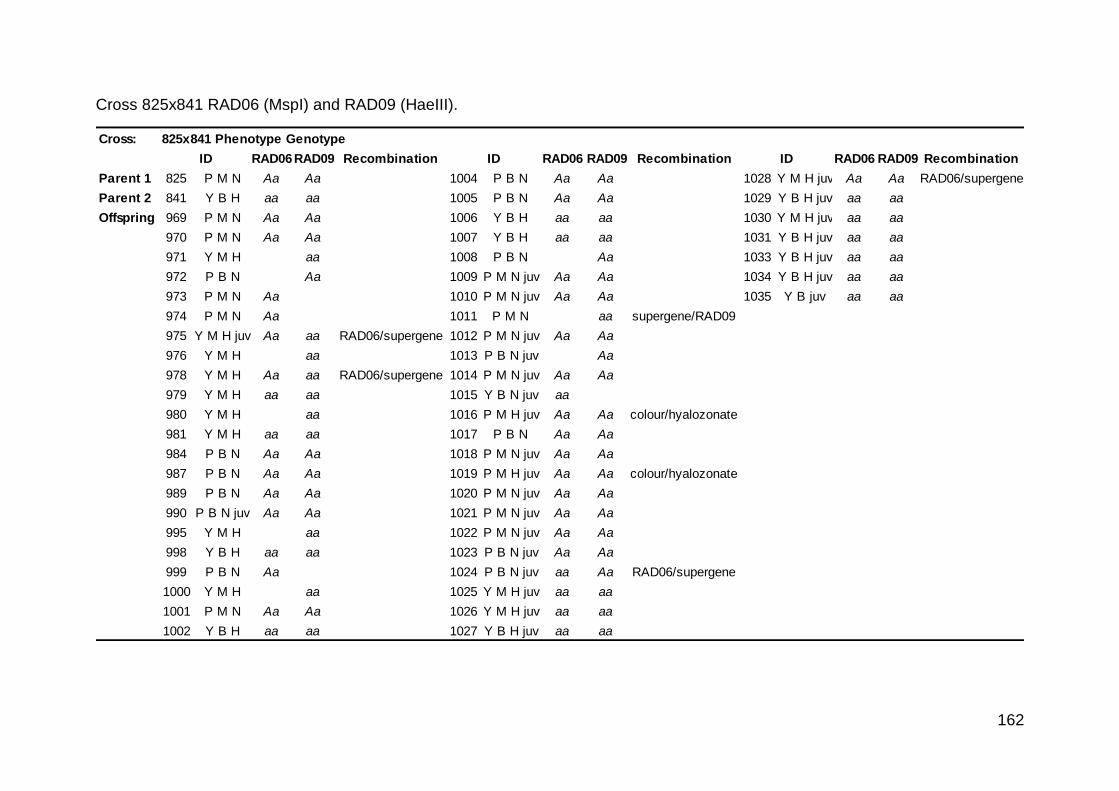
162
Cross 825x841 RAD06 (MspI) and RAD09 (HaeIII).
Cross: 825x841 Phenotype Genotype
RAD06RAD09 Recombination RAD06 RAD09 Recombination RAD06 RAD09 Recombination
Parent 1 825 P M N Aa Aa 1004 P B N Aa Aa 1028 Y M H juv Aa Aa RAD06/supergene
Parent 2 841 Y B H aa aa 1005 P B N Aa Aa 1029 Y B H juv aa aa
Offspring 969 P M N Aa Aa 1006 Y B H aa aa 1030 Y M H juv aa aa
970 P M N Aa Aa 1007 Y B H aa aa 1031 Y B H juv aa aa
971 Y M H aa 1008 P B N Aa 1033 Y B H juv aa aa
972 P B N Aa 1009 P M N juv Aa Aa 1034 Y B H juv aa aa
973 P M N Aa 1010 P M N juv Aa Aa 1035 Y B juv aa aa
974 P M N Aa 1011 P M N aa supergene/RAD09
975 Y M H juv Aa aa RAD06/supergene 1012 P M N juv Aa Aa
976 Y M H aa 1013 P B N juv Aa
978 Y M H Aa aa RAD06/supergene 1014 P M N juv Aa Aa
979 Y M H aa aa 1015 Y B N juv aa
980 Y M H aa 1016 P M H juv Aa Aa colour/hyalozonate
981 Y M H aa aa 1017 P B N Aa Aa
984 P B N Aa Aa 1018 P M N juv Aa Aa
987 P B N Aa Aa 1019 P M H juv Aa Aa colour/hyalozonate
989 P B N Aa Aa 1020 P M N juv Aa Aa
990 P B N juv Aa Aa 1021 P M N juv Aa Aa
995 Y M H aa 1022 P M N juv Aa Aa
998 Y B H aa aa 1023 P B N juv Aa Aa
999 P B N Aa 1024 P B N juv aa Aa RAD06/supergene
1000 Y M H aa 1025 Y M H juv aa aa
1001 P M N Aa Aa 1026 Y M H juv aa aa
1002 Y B H aa aa 1027 Y B H juv aa aa
ID ID ID

163
Cross 118x119 RAD8 (HinfI) and RAD10 (DpnII).
Cross: 118x119 Phenotype Genotype
RAD8 RAD10 Recombination RAD8 RAD10 Recombination RAD8 RAD10 Recombination
Parent 1 118 Y M aa aa 462 Y M Aa Aa 398 P M aa aa
Parent 2 119 P M Aa Aa 463 Y M Aa Aa 399 P M aa aa
Offspring 353 Y M Aa Aa 465 Y M Aa Aa 410 P M aa aa
354 Y M Aa Aa 466 Y M Aa Aa 411 P M aa aa
355 Y M Aa Aa 468 Y M Aa Aa 415 P M aa aa
356 Y M Aa Aa 538 Y M Aa Aa 417 P M aa aa
391 Y M Aa Aa 539 Y M Aa Aa 419 P M aa aa
392 Y M Aa Aa 540 Y M Aa Aa 420 P M aa aa
393 Y M Aa Aa 469 Y M Aa Aa 453 P M aa aa
400 Y M Aa Aa 470 Y M Aa Aa 454 P M aa aa
412 Y M Aa Aa 471 Y M Aa Aa 455 P M aa aa
413 Y M Aa Aa 472 Y M Aa Aa 456 P M aa aa
414 Y M Aa Aa 473 Y M Aa Aa 457 P M aa aa
418 Y M Aa Aa 474 Y M Aa Aa 458 P M aa aa
421 Y M Aa Aa 357 P M aa aa 459 P M aa aa
432 Y M Aa Aa 358 P M aa aa 460 P M aa aa
433 Y M Aa Aa 359 P M aa aa 541 P M aa aa
434 Y M Aa Aa 360 P M aa aa 542 P M aa aa
435 Y M Aa Aa 361 P M aa aa 543 P M aa aa
436 Y M Aa Aa 362 P M aa aa 416 P M aa aa
437 Y M Aa Aa 394 P M aa aa
438 Y M Aa Aa 395 P M aa aa
439 Y M Aa Aa 396 P M aa aa
461 Y M Aa Aa 397 P M aa aa
ID ID ID

164
Cross 104x105 all markers were homozygous. Thus, not informative results came out of this offspring.
Cross: 104x105 Phenotype Genotype
Parent 1 104 P O All markers homozygous - not informative 329 P O
Parent 2 105 Y M 330 P O
Offspring 192 P O 331 P O
193 P O 332 P O
194 P O 333 P O
197 P O 118 Y M
198 P O 178 Y M
199 P O 179 Y M
200 P O 180 Y M
256 P O 181 Y M
257 P O 201 Y M
321 P O 202 Y M
322 P O 249 Y M
323 P O 250 Y M
324 P O 251 Y M
327 P O 252 Y M
328 P O 254 Y M
334 P O 317 Y M
401 P O 402 Y M
195 P O 203 Y M
196 P O 253 Y M
255 P O 318 Y M
325 P O 319 Y M
326 P O 320 Y M
ID ID

165
Table S2.4. Inferred genotypes of all individuals. Shells with a phenotype that may be due to a potential recombination event in
parent are shown in bold.
Locus Parent 1 Parent 2 Offspring
Cross #1 C100 C101
Phenotype P O x Y M Sum P M Y O
103 56 47
Genotype Colour CP
CY
CY
CY
CP
CY
CY
CY
Banding B B B O B B B B B B B B B O B B
Mid-band U 3 U 3 U 3 U 3/- U 3 U 3/- U 3 U 3/-
Cross #2 C102 C103
Phenotype P O x Y M Sum P O Y M Y O
43 20 20 3
Genotype Colour C P C Y C Y C Y C P C Y C Y C Y C P C Y
Banding B O B B B B B B B O B B B B B B B B B B
Mid-band U 3 U 3 U 3/- U 3/- U 3 U 3/- U 3 U 3/- U 3 U 3/-
Cross #3 C104 C105
Phenotype P O x Y M Sum P O Y M
46 27 19
Genotype Colour CP
CY
CY
CY
CP
CY
CY
CY
Banding B O B B B B B B B O B B B B B B
Mid-band U 3 U 3 U 3/- U 3/- U 3 U 3/- U 3 U 3/-
Cross #4 C110 C111
Phenotype P O x Y B Sum P B Y O
27 17 10
Genotype Colour C P C Y C Y C Y C P C Y C Y C Y
Banding B B B O B B B B B B B B B O B B
Mid-band U - U - U - U - U - U - U - U -

166
Cross #5 C112 C113
Phenotype P O x Y B (12345)Sum P B (00345) P B (12345)P B (02345)Y O P M
109 27 12 16 53 1
Genotype Colour C P C Y C Y C Y C P C Y C P C Y C P C Y C Y C Y C P C Y
Banding BB
BO
BB
Bb
BB
BB
BB
BB
BB
BB
BO
BB
BB
BB
Mid-band U - U - U - U - U - U - U - U - U - U - U - U - U - U -
00345-band T 345T ─ T ─ T ─ T 345
T ─ T ─ T ─ T ─ T ─ T 345/-T ─
02345-band X 2345X ─ X ─ X ─ X 2345/-
X ─ X ─ X ─ X 2345X ─ X 2345
X ─
Cross #6 C114 C115
Phenotype P O x Y B Sum P O Y B Y M
34 18 8 8
Genotype Colour CP
CY
CY
CY
CP
CY
CY
CY
CY
CY
Banding B O B B B B B B B O B B B B B B B B B B
Mid-band U 3 U - U - U - U 3 U - U - U - U 3 U -
Cross #7 C118 C119
Phenotype P M x Y M Sum P M Y M
75 37 38
Genotype Colour C P C Y C Y C Y C P C Y C Y C Y
Mid-band U3
U3/-
U3
U3/-
U3
U3/-
U3
U3/-
Cross #8 C108 C109
Phenotype P O L x Y M L Sum P M L Y O L Y O A P O L
50 26 11 12 1
Genotype Colour C P C Y C Y C Y C P C Y C Y C Y C Y C Y C P C Y
Banding B B B O B B B B B B B B B O B B B O B B B O B B
Lip LL LA LL LA LL LL/A LA L L LA LA LL LA
Mid-band U 3 U 3 U 3 U - U 3 U 3/- U 3 U 3/- U 3 U 3/- U 3 U 3/-

167
Cross #9 C116 C120
Phenotype P M N x Y B H Sum P M N P B N Y M N Y B N
16 4 4 3 5
Genotype Colour C P C Y C Y C Y C P C Y C P C Y C Y C Y C Y C Y
Banding B B B B B B B B B B B B B B B B B B B B B B B B
Band pigmentation P N P N P H P H P N P H P N P H P N P H P N P H
Mid-band U 3 U - U - U - U 3 U - U - U - U 3 U - U - U -
Cross #10 C450 C449
Phenotype P M N x Y B N Sum P M N P B N Y M N Y B N Y M H Y B H
12 5 2 2 1 2 0
Genotype Colour C P C Y C Y C Y C P C Y C P C Y C Y C Y C Y C Y C Y C Y C Y C Y
Banding B B B B B B B B B B B B B B B B B B B B B B B B B B B B B B B B
Band pigmentation P N P H P N P H P N P N/H P N P N/HP N P H P N P H P H P H P H P H
Mid-band U3
U-
U-
U-
U3
U-
U-
U-
U3
U-
U-
U-
U3
U-
U-
U-
Cross #11 C451 C452
Phenotype P M N x Y B N Sum P M N P B N Y M N Y B N Y M H Y B H P M H
116 34 28 12 22 10 6 4
Genotype Colour CP
CY
CY
CY
CP
CY
CP
CY
CY
CY
CY
CY
CY
CY
CY
CY
CP
CY
Banding B B B B B B B B B B B B B B B B B B B B B B B B B B B B B B B B B B B B
Band pigmentation P N P H P N P H P N P N/H P N P N P N P H P N P H P H P H P H P H P H P H
Mid-band U 3 U - U - U - U 3 U - U - U - U 3 U - U - U - U 3 U - U - U - U 3 U -
Cross #12 C662 C665
Phenotype P M N x Y B N Sum P M N P B N Y M N Y B N Y M H Y B H P M H
146 39 46 7 19 15 12 8
Genotype Colour C P C Y C Y C Y C P C Y C P C Y C Y C Y C Y C Y C Y C Y C Y C Y C P C Y
Banding B B B B B B B B B B B B B B B B B B B B B B B B B B B B B B B B B B B B
Band pigmentation P N P H P N P H P N P H P N P N P N P H P N P H P H P H P H P H P H P H
Mid-band U 3 U - U - U - U 3 U - U - U - U 3 U - U - U - U 3 U - U - U - U 3 U -

168
Cross #13 C825 C841
Phenotype P M N x Y B H Sum P M N P B N Y M N Y B N Y M H Y B H P M H
63 14 18 0 0 20 9 2
Genotype Colour C P C Y C Y C Y C P C Y C P C Y C Y C Y C Y C Y C Y C Y C Y C Y C P C Y
Banding B B B B B B B B B B B B B B B B B B B B B B B B B B B B B B B B B B B B
Band pigmentation P N P H P H P H P N P H P N P H P N P H P N P H P H P H P H P H P H P H
Mid-band U 3 U - U - U - U 3 U - U - U - U 3 U - U - U - U 3 U - U - U - U 3 U -
Cross #14 C568 C569
Phenotype Y B (12345) x Y O Sum Y B (12345) Y O
44 28 16
Genotype Colour C Y C Y C Y C Y C Y C Y C Y C Y
Banding B B B B B O B B B B B B B O B B
Spread-banding S S S S S - S - S S S - S - S S
Mid-band U - U - U - U - U - U - U - U -

169
Chapter 3:
Figure S3.1. The following density graphs illustrate the quality of the vcf file. Phred
quality score (top-left), the variant mean depth (top-right), individual missing data
(centre-left) and the variant missing data (centre-right) for each loci were plotted.
Minor allele frequency density graphs of the entire variant calling data (bottom-left)
and the filtered file (bottom-right) are illustrated. Filtering removed all the loci with
minor allele frequency lower or equal to 10% ruling out possible genotyping error
rates and invariant loci.
Figure S3.2. Correlation between contig length and the number of SNPs present in
the whole-genome dataset.
Figure S3.3. The proportion of the variation explained by each axis returned by the
principal components analysis.
Figure S3.4. Cross validation error results for each admixture group (K).
Table S3.1. Illumina reads sequenced per individual and allelic coverage of the
double restriction site–associated DNA (RAD) loci dataset.
Table S3.2. Contigs surrounding the supergene described by Dr. Suzanne Saenko,
RAD-seq loci mapping supergene-linked contigs and supergene-linked contigs (with
their RAD-seq loci started position) presenting SNP's in the filtered dataset and their
SNP's position.
Table S.3.3. PCA data for the whole-genome dataset.
Table S.3.4. All contigs present in the final dataset showing their length and number
of SNPs. Moreover, Mantel test results between genetic distance of each RAD
genomic regions and the geographical distance.
Supplementary Material: The allelic balance at heterozygotes to detect
contamination for each sample can be access by request.

170
Figure S3.1. Quality checks of the variant calling dataset and filtering.

171
Figure S3.2. Correlation between contig length and the number of SNPs present in the whole-
genome dataset.

172
Figure S3.3. The proportion of the variation explained by each axis returned by the principal components analysis.

173
Figure S3.4. Cross validation error results for each admixture group (K).

174
ID samples HQ reads HQ reads mapped to reference % reads mapped to reference ./. 0/0 0/1 1/1
26 8849929 8441460 0.95 1861 3835 1231 1755
27 7719430 7382608 0.96 1709 4054 1097 1816
28 5375147 5133507 0.96 1864 4080 1198 1531
29 8984822 8611299 0.96 1216 4414 1367 1679
30 6930986 6530062 0.94 1954 3268 1017 2436
31 7148020 6868309 0.96 983 4200 1375 2114
32 8108195 7679710 0.95 1518 3699 1250 2207
33 8484716 8049748 0.95 1364 3907 1258 2141
34 8893638 8449811 0.95 1476 3883 1057 2259
35 10029342 9499300 0.95 1821 3281 1142 2427
36 8517263 8160706 0.96 1708 3776 1099 2098
37 6564917 6220633 0.95 1714 3786 1095 2084
38 4831810 4617760 0.96 3284 2966 804 1630
39 4246532 3982228 0.94 2999 3144 870 1666
40 9898068 9440156 0.95 1591 3886 1202 2000
41 7803244 7436938 0.95 1685 3648 1075 2267
42 8559966 7946228 0.93 2153 3398 647 2478
43 4244115 3909122 0.92 3093 2904 799 1881
44 8127575 7458672 0.92 1862 3528 909 2374
45 10456078 9967158 0.95 1194 4028 1483 1973
46 6833045 6582555 0.96 1395 4348 1061 1873
47 6327893 6097916 0.96 1699 4181 989 1812
48 9159767 8690192 0.95 1121 4647 1281 1630
49 7681527 7369040 0.96 1062 4537 1310 1768
50 7770439 7427688 0.96 1242 4230 1195 2008
Genotype count final dataset
Table S3.1. Illumina reads sequenced per individual and allelic coverage of the double restriction site–associated DNA (RAD)
loci dataset.

175
51 1896319 1824665 0.96 3113 3302 959 1304
52 8045555 7750617 0.96 1257 4520 1128 1771
53 7050933 6767607 0.96 1649 4187 1044 1800
54 7992130 7683529 0.96 900 4537 1314 1929
55 9381678 8877341 0.95 1374 3562 1230 2507
56 5344676 5068577 0.95 1105 3944 1463 2159
57 188180 - - - - - -
58 58766 - - - - - -
59 6123971 5874845 0.96 1166 4008 1260 2241
60 7544753 7211956 0.96 892 3586 1601 2587
61 6842140 6583604 0.96 1262 4027 1102 2282
62 2008007 1912867 0.95 3894 2597 707 1480
63 8119802 7688658 0.95 1667 3751 1239 2019
64 6463278 6129393 0.95 1945 3679 1131 1923
65 6384347 6050609 0.95 2428 3079 1077 2096
66 7585286 7232495 0.95 1519 4080 1165 1915

176
Supergene Contigs RAD-seq Supergene contigs RAD-seq supergene variant (Starting-pos) RAD-seq supergene SNPs
ctg61795 ctg61795 ctg18101-31427 ctg18101-31462
ctg57160 ctg57160 ctg7799-57269 ctg18101-31485
ctg57388 ctg57388 ctg6465-72273 ctg18101-31487
ctg52372 ctg52372 ctg10711-128872 ctg18101-31497
ctg46636 ctg46636 tig00001874-209300/209316 ctg18101-31568
ctg45378 ctg45378 tig02170041 (RAD8/10)-201334 ctg7799-57301
ctg41688 ctg41688 tig00045252-71 ctg7799-57375
ctg40857 ctg40857 ctg6465-72280
ctg38937 ctg38937 ctg6465-72292
ctg33047 ctg33047 ctg6465-72313
ctg33079 ctg33079 ctg6465-72337
ctg31172 ctg31172 ctg6465-72351
ctg30377 ctg30377 ctg6465-72417
ctg29158 ctg29158 ctg10711-128947
ctg26173 ctg26173 ctg10711-128949
ctg22062 ctg22062 ctg10711-128990
ctg29028 ctg29028 ctg10711-129013
ctg23215 ctg23215 tig00001874-209360
ctg19577 ctg19577 tig00001874-209405
ctg26823 (RAD06) ctg26823 (RAD06) tig00001874-209411
ctg18462 ctg18462 tig00001874-209414
ctg18261 ctg18261 tig00001874-209423
ctg27326 ctg27326 tig00001874-209432
ctg31541 ctg31541 tig02170041-203393
ctg14665 ctg14665 tig02170041-203394
Table S3.2. Contigs surrounding the supergene described by Dr. Suzanne Saenko, RAD-seq loci mapping supergene-linked
contigs and supergene-linked contigs (with their RAD-seq loci started position) presenting SNP's in the filtered dataset and
their SNP's position.

177
ctg15079 ctg15079 tig02170041-203482
ctg14676 ctg14676 tig00045252-132
ctg10733 ctg10733 tig00045252-137
ctg15298 ctg15298 tig00045252-141
ctg9575 ctg9575 tig00045252-207
ctg8491 ctg8491 tig00045252-209
ctg4892 ctg4892
ctg12182 ctg12182
ctg39989
ctg23821
ctg18101
ctg15973
ctg29354
ctg14244
ctg15341
ctg16135
ctg7799
ctg6901
ctg12782
ctg5603 (RAD06)
ctg6465
ctg20315
ctg7855
ctg7898
ctg10711
contig_18515
tig02169229
ctg5701 (RAD9)
ctg8479

178
ctg6294
tig00001874
tig02170041 (RAD8/10)
tig00398893
tig00012620
tig00045252

179
Table S3.3. PCA data for the whole-genome dataset.
ID PC1 PC2 PC3 PC4 PC5 PC6 PC7 PC8 PC9 PC10 PC11 PC12 PC13 PC14 PC15 PC16
26 0.155 0.080 0.041 -0.040 0.529 -0.196 0.297 -0.139 -0.170 -0.053 0.023 0.037 0.013 -0.037 0.040 0.017
27 0.136 0.076 0.054 0.082 0.072 -0.018 -0.175 0.200 0.088 0.055 0.780 -0.237 -0.005 -0.288 -0.017 0.153
28 0.154 0.074 0.032 -0.062 0.095 -0.076 -0.210 0.125 0.192 0.267 -0.197 -0.132 0.038 -0.008 -0.043 -0.459
29 0.166 0.109 0.057 -0.122 0.087 -0.128 -0.209 0.062 0.134 0.223 -0.078 -0.153 0.049 -0.044 -0.017 -0.281
30 -0.279 0.149 -0.221 -0.050 0.050 -0.156 -0.042 0.000 0.030 -0.072 0.013 -0.040 -0.062 0.026 0.037 -0.035
31 0.073 0.034 0.002 0.095 -0.035 -0.116 -0.050 0.091 -0.088 0.347 -0.338 -0.317 0.213 -0.311 -0.180 0.318
32 0.026 -0.321 -0.096 -0.059 0.004 0.031 0.057 -0.020 0.043 -0.136 0.137 -0.033 0.011 -0.006 -0.204 -0.333
33 0.013 -0.308 -0.082 -0.010 0.022 0.017 0.049 -0.099 0.015 -0.082 0.021 -0.011 0.118 0.068 -0.267 -0.254
34 0.026 -0.324 -0.129 -0.085 -0.033 0.003 0.021 0.098 0.024 -0.142 -0.104 -0.133 0.057 -0.110 -0.021 0.115
35 -0.270 0.144 -0.244 -0.022 -0.020 -0.142 -0.068 -0.025 0.054 -0.022 0.004 0.013 -0.020 -0.006 0.055 0.011
36 0.040 -0.001 -0.020 0.500 0.024 0.113 -0.057 -0.207 0.125 -0.020 -0.118 -0.175 -0.159 0.045 0.174 0.005
37 0.039 -0.013 -0.015 0.527 0.072 0.122 -0.082 -0.157 0.050 -0.068 -0.044 -0.207 -0.204 0.100 0.154 0.017
38 0.070 0.066 0.007 0.280 0.045 0.072 -0.079 0.515 -0.089 -0.154 -0.142 0.345 0.089 -0.096 0.029 -0.027
39 0.061 0.049 0.041 0.268 0.060 0.072 -0.035 0.390 -0.191 -0.095 0.008 0.288 0.162 0.192 -0.137 -0.078
40 -0.033 0.137 -0.018 -0.167 -0.004 0.570 0.144 -0.030 -0.011 0.060 0.019 0.038 -0.125 -0.118 0.029 -0.046
41 -0.188 0.111 -0.069 0.039 -0.046 0.195 0.193 -0.047 -0.213 0.117 -0.045 -0.114 0.067 -0.100 -0.348 0.013
42 -0.325 -0.096 0.467 -0.032 -0.004 -0.061 0.015 0.033 0.031 -0.015 -0.020 -0.022 -0.025 -0.006 0.015 0.045
43 -0.277 -0.073 0.436 -0.029 -0.012 -0.030 -0.003 0.003 -0.021 -0.054 -0.012 -0.020 0.025 0.002 0.068 -0.050
44 -0.301 -0.078 0.447 -0.023 0.009 -0.049 -0.032 0.029 0.016 -0.014 0.002 -0.040 -0.036 0.009 0.005 -0.012
45 -0.031 0.144 -0.013 -0.134 -0.017 0.484 0.156 0.008 -0.133 0.043 -0.038 -0.036 -0.083 -0.247 0.186 -0.165
46 0.169 0.099 0.066 -0.070 -0.205 -0.097 -0.241 -0.296 -0.379 -0.091 -0.028 0.070 0.041 -0.028 -0.004 -0.133
47 0.162 0.105 0.080 -0.033 -0.219 -0.038 -0.286 -0.279 -0.458 -0.141 0.081 0.039 0.176 -0.014 0.086 0.056
48 0.180 0.071 0.064 -0.210 0.072 0.071 -0.219 -0.040 0.268 -0.132 0.043 0.131 -0.161 0.061 0.224 -0.056
49 0.161 0.084 0.037 -0.198 0.015 0.111 -0.131 -0.031 0.261 -0.163 -0.167 0.102 0.045 -0.052 -0.173 0.198
50 0.077 0.130 0.026 -0.097 -0.088 0.190 0.105 0.068 0.026 0.155 0.104 -0.285 0.277 0.750 -0.015 0.129
51 0.114 0.101 0.050 -0.182 -0.005 0.037 -0.055 -0.010 0.264 -0.185 -0.153 0.120 0.089 -0.003 0.016 0.376
52 0.170 0.102 0.063 -0.038 -0.133 -0.147 0.064 0.075 -0.084 -0.072 -0.034 -0.017 -0.713 0.158 -0.477 0.107
53 0.135 0.111 0.036 0.079 -0.377 -0.203 0.417 0.019 0.155 -0.035 0.015 0.036 0.074 -0.088 0.134 -0.123
54 0.130 0.102 0.026 0.070 -0.390 -0.209 0.395 -0.019 0.171 0.007 0.060 0.081 0.076 -0.071 0.151 -0.071
55 -0.271 0.166 -0.226 -0.028 0.023 -0.097 -0.042 -0.015 0.012 -0.028 0.031 0.033 -0.069 0.039 0.014 0.025

180
56 0.024 -0.305 -0.116 -0.063 -0.056 0.021 0.061 0.024 -0.019 -0.150 0.036 -0.111 0.015 -0.130 -0.059 0.043
59 -0.048 -0.133 -0.019 0.214 0.044 0.107 -0.069 -0.401 0.310 -0.004 0.059 0.273 0.253 -0.028 -0.270 0.075
60 -0.261 0.161 -0.240 -0.022 0.012 -0.105 -0.038 0.002 0.049 0.025 -0.006 0.056 -0.008 -0.020 -0.024 0.025
61 0.034 -0.327 -0.126 -0.099 -0.011 -0.034 -0.028 0.096 -0.128 -0.070 -0.094 -0.117 -0.103 0.115 0.274 -0.040
62 0.034 -0.269 -0.122 -0.104 -0.020 -0.016 -0.010 0.149 -0.082 -0.050 -0.100 -0.119 -0.039 0.019 0.269 0.244
63 0.009 -0.204 -0.075 -0.035 -0.041 0.011 0.003 0.041 -0.064 0.331 0.240 0.259 -0.012 0.097 -0.005 0.134
64 -0.013 -0.196 -0.037 -0.006 -0.015 -0.044 -0.043 -0.110 -0.043 0.589 -0.013 0.402 -0.196 0.033 0.156 0.082
65 -0.249 0.147 -0.215 -0.048 0.016 -0.103 -0.100 0.038 -0.033 -0.120 0.046 -0.011 0.097 0.067 0.038 -0.079
66 0.145 0.073 0.054 -0.044 0.506 -0.141 0.317 -0.123 -0.115 -0.029 -0.003 0.030 0.061 0.029 0.065 0.046

181
Table S3.4. All contigs present in the final dataset showing their length and number of SNPs. Moreover, Mantel test results
between genetic distance of each RAD genomic regions and the geographical distance.
scaffold Contig Length SNPs Fst mean Mantel r P-value ctg10711 214766 4 0.299 0.010 0.274 ctg18101 41596 5 0.403 -0.003 0.529
ctg6465 130785 6 0.108 0.102 0.000
ctg7799 89027 2 0.281 0.002 0.454
tig00001874 347208 6 0.192 0.040 0.010
tig00045252 1171230 5 0.173 -0.009 0.621
tig02170041 440716 3 0.255 0.004 0.406
ctg5276 175985 1 0.135 -0.170 1.000
tig00041043 748783 1 0.137 -0.137 1.000
ctg7924 404164 1 0.066 -0.125 1.000
ctg6606 147718 1 0.112 -0.123 1.000
contig_23319 289200 3 0.205 -0.122 1.000
tig02186502 521409 1 0.170 -0.110 1.000
tig00054407 676461 1 0.125 -0.106 1.000
ctg18483 39850 1 0.189 -0.106 1.000
tig00401724 386201 2 0.220 -0.102 1.000
ctg6765 98076 1 0.131 -0.102 1.000
ctg291 466624 2 0.170 -0.101 1.000
ctg6031 104614 3 0.155 -0.101 1.000
tig00402053 412341 1 0.132 -0.101 1.000
ctg13598 116761 3 0.174 -0.100 1.000
ctg44666 12839 1 0.148 -0.100 1.000
ctg12314 121369 8 0.190 -0.099 1.000
contig_53782 638023 3 0.248 -0.097 1.000
ctg1015 337978 1 0.082 -0.096 1.000
tig00405312 546268 1 0.150 -0.096 1.000
ctg20106 104214 10 0.170 -0.089 1.000
tig00397172 347118 2 0.209 -0.088 1.000
ctg7192 240187 2 0.074 -0.084 1.000
contig_689 476457 2 0.227 -0.084 1.000
tig00050418 273796 4 0.163 -0.082 1.000
tig00396244 1834507 9 0.207 -0.080 1.000
tig00040990 955367 2 0.174 -0.079 1.000
tig00005194 612128 1 0.261 -0.078 1.000
tig00024280 522037 3 0.341 -0.061 1.000
tig00008071 418812 2 0.235 -0.058 1.000
tig00021475 252673 1 0.090 -0.112 1.000
tig00407665 258132 1 0.067 -0.097 1.000
ctg6557 190769 1 0.206 -0.085 1.000
ctg145 513807 1 0.171 -0.084 1.000
tig00015817 424690 2 0.125 -0.079 1.000
ctg6752 174357 1 0.233 -0.078 1.000
ctg3436 146131 2 0.243 -0.073 1.000
ctg4188 293217 5 0.197 -0.068 1.000
ctg1258 369546 1 0.270 -0.068 1.000
ctg6325 141808 6 0.310 -0.061 1.000
tig00398538 452927 1 0.174 -0.078 1.000
contig_431 589511 2 0.231 -0.068 1.000
tig00009358 809549 4 0.278 -0.055 1.000
scaffold_32099 454066 1 0.130 -0.090 1.000
tig02186388 759101 14 0.260 -0.070 1.000
ctg1210 716347 4 0.211 -0.063 1.000
tig00006570 592824 3 0.291 -0.063 1.000
contig_4695 367886 6 0.348 -0.055 1.000
ctg5838 108313 2 0.373 -0.044 1.000
ctg1474 382591 1 0.172 -0.082 1.000
contig_52177 222994 2 0.212 -0.066 1.000
tig00396812 424463 5 0.276 -0.059 1.000
ctg4789 236449 3 0.206 -0.052 1.000
tig00403009 398319 1 0.105 -0.099 1.000
ctg2428 334772 1 0.127 -0.088 1.000

182
ctg6981 161642 5 0.283 -0.064 1.000
tig00036448 352128 2 0.272 -0.051 1.000
ctg46545 13873 5 0.196 -0.071 0.999
tig00399345 573471 7 0.189 -0.068 0.999
ctg1969 249935 3 0.257 -0.057 0.999
tig00397759 417826 1 0.260 -0.057 0.999
ctg1729 227373 5 0.271 -0.045 0.999
ctg1327 304415 8 0.205 -0.034 0.999
scaffold_56103 419285 1 0.251 -0.055 0.998
tig02186840 468967 1 0.169 -0.075 0.998
tig00119532 356718 1 0.228 -0.064 0.998
tig00006926 902723 2 0.292 -0.054 0.998
ctg6571 149310 4 0.143 -0.075 0.998
tig00002546 437028 4 0.251 -0.048 0.998
tig00057919 436433 8 0.210 -0.047 0.998
ctg11117 106448 7 0.265 -0.056 0.997
ctg2051 206267 6 0.204 -0.051 0.997
tig02171594 616023 3 0.238 -0.044 0.997
ctg30048 105587 3 0.223 -0.034 0.997
tig00010953 659108 6 0.158 -0.060 0.997
ctg1262 473267 1 0.315 -0.043 0.997
ctg778 822759 6 0.222 -0.043 0.997
ctg40795 15483 3 0.184 -0.055 0.997
contig_27674 345663 2 0.208 -0.059 0.997
ctg1130 244509 3 0.217 -0.048 0.997
ctg2231 323080 4 0.180 -0.047 0.997
ctg3672 177353 16 0.360 -0.043 0.997
ctg3589 135977 17 0.198 -0.061 0.997
tig00406272 924428 1 0.259 -0.050 0.996
ctg3197 425979 1 0.316 -0.043 0.996
contig_27294 397769 4 0.445 -0.032 0.996
tig00005735 943713 5 0.177 -0.056 0.996
tig00006949 1521481 17 0.297 -0.045 0.996
contig_1838 281150 1 0.112 -0.074 0.995
ctg52391 9703 8 0.327 -0.041 0.995
ctg7429 139935 8 0.201 -0.042 0.995
ctg5571 143972 6 0.265 -0.051 0.995
tig00004394 1026468 3 0.146 -0.051 0.995
ctg4160 417727 2 0.288 -0.047 0.995
tig00046703 666969 3 0.256 -0.045 0.995
ctg6030 288957 2 0.219 -0.033 0.995
tig00053952 273129 1 0.338 -0.031 0.995
ctg7750 138288 2 0.195 -0.049 0.995
tig02170482 275430 1 0.236 -0.055 0.995
tig00038242 363803 2 0.118 -0.073 0.994
contig_18474 427180 3 0.183 -0.064 0.994
ctg34037 20530 4 0.111 -0.068 0.994
ctg518 409262 4 0.262 -0.042 0.994
ctg15951 66240 5 0.172 -0.057 0.994
ctg13923 53982 5 0.322 -0.050 0.994
tig02170140 733074 5 0.165 -0.048 0.993
tig02187252 680965 5 0.294 -0.047 0.993
contig_40511 233997 3 0.198 -0.058 0.993
ctg4236 198866 10 0.260 -0.043 0.993
ctg32976 35090 1 0.230 -0.053 0.992
ctg8508 149018 2 0.196 -0.047 0.992
tig02176378 1070279 2 0.124 -0.054 0.992
ctg1705 399091 5 0.385 -0.030 0.992
contig_4524 340071 4 0.342 -0.045 0.992
contig_15272 814290 2 0.252 -0.052 0.992
scaffold_46834 290133 2 0.100 -0.047 0.992
tig02171663 620512 1 0.210 -0.051 0.991
ctg125 701017 6 0.320 -0.040 0.991
contig_25791 989377 1 0.113 -0.069 0.991

183
ctg11116 222084 1 0.276 -0.048 0.991
tig00093181 974712 5 0.283 -0.040 0.990
ctg14575 51019 3 0.264 -0.047 0.990
ctg2370 427969 1 0.096 -0.062 0.990
tig00399423 661880 1 0.234 -0.054 0.990
ctg1840 356731 1 0.330 -0.037 0.989
ctg317 865042 2 0.365 -0.037 0.989
ctg22032 68149 1 0.254 -0.046 0.988
tig02171538 366358 10 0.233 -0.045 0.988
ctg16248 47162 3 0.269 -0.044 0.988
ctg498 528509 1 0.044 -0.067 0.988
ctg1811 477430 7 0.194 -0.043 0.988
ctg6639 160573 4 0.422 -0.026 0.988
ctg13069 99907 1 0.150 -0.064 0.988
tig00007057 1324150 1 0.249 -0.047 0.988
ctg39323 17110 1 0.238 -0.049 0.987
tig00028358 406162 4 0.314 -0.039 0.987
tig00032819 433670 1 0.141 -0.056 0.987
ctg28552 29826 1 0.165 -0.055 0.987
tig00399328 437189 2 0.221 -0.049 0.987
ctg6944 433447 5 0.438 -0.012 0.986
contig_26754 357624 1 0.277 -0.041 0.986
contig_19330 830498 6 0.183 -0.033 0.986
ctg7749 108123 6 0.255 -0.043 0.985
tig00009350 799186 1 0.343 -0.031 0.985
tig00064007 342934 1 0.144 -0.058 0.985
ctg4207 284892 2 0.250 -0.045 0.985
ctg4983 330389 1 0.058 -0.067 0.985
ctg51856 10423 2 0.261 -0.046 0.985
contig_61810 613156 3 0.302 -0.033 0.984
ctg5129 119983 2 0.276 -0.042 0.984
tig00397802 696041 2 0.136 -0.059 0.984
tig00031716 616509 4 0.298 -0.039 0.984
tig00016167 1008196 2 0.239 -0.047 0.984
ctg8197 97348 1 0.183 -0.056 0.984
ctg2160 487772 1 0.181 -0.056 0.983
tig00399075 411201 20 0.254 -0.042 0.983
ctg8810 115513 2 0.106 -0.056 0.983
tig00398828 850437 8 0.208 -0.039 0.982
tig00041084 252056 1 0.125 -0.060 0.982
ctg10194 72179 2 0.264 -0.043 0.982
contig_8740 463624 3 0.390 -0.026 0.981
tig00397755 229364 2 0.255 -0.040 0.981
contig_6833 679942 12 0.321 -0.042 0.981
scaffold_59590 510281 2 0.336 -0.030 0.981
tig00396865 961683 4 0.395 -0.026 0.981
contig_53681 1302649 10 0.233 -0.031 0.980
ctg4944 223218 2 0.175 -0.047 0.980
contig_1774 895011 15 0.387 -0.036 0.980
ctg1861 247159 1 0.156 -0.048 0.979
tig00024223 665328 2 0.183 -0.051 0.978
tig02169800 615581 1 0.110 -0.044 0.978
contig_17623 686403 2 0.221 -0.035 0.977
contig_35656 409111 7 0.233 -0.041 0.977
ctg8224 340785 8 0.299 -0.036 0.976
contig_7543 649077 3 0.204 -0.035 0.976
tig00066007 320286 10 0.184 -0.038 0.976
tig00005910 857596 1 0.226 -0.045 0.976
ctg2887 255917 1 0.159 -0.052 0.975
tig00398326 606047 2 0.340 -0.032 0.975
ctg14959 117517 2 0.066 -0.058 0.975
tig02187655 457626 9 0.378 -0.029 0.975
tig00398865 1094907 8 0.146 -0.038 0.974
tig00001599 1569036 2 0.203 -0.039 0.973
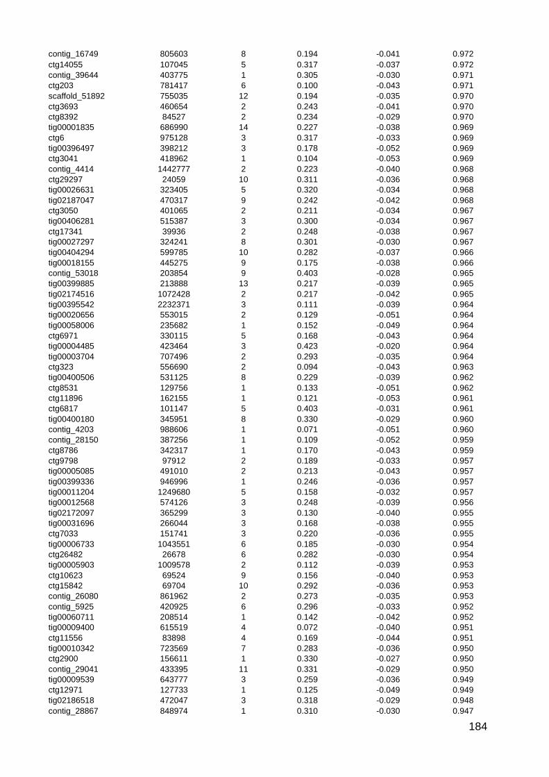
184
contig_16749 805603 8 0.194 -0.041 0.972
ctg14055 107045 5 0.317 -0.037 0.972
contig_39644 403775 1 0.305 -0.030 0.971
ctg203 781417 6 0.100 -0.043 0.971
scaffold_51892 755035 12 0.194 -0.035 0.970
ctg3693 460654 2 0.243 -0.041 0.970
ctg8392 84527 2 0.234 -0.029 0.970
tig00001835 686990 14 0.227 -0.038 0.969
ctg6 975128 3 0.317 -0.033 0.969
tig00396497 398212 3 0.178 -0.052 0.969
ctg3041 418962 1 0.104 -0.053 0.969
contig_4414 1442777 2 0.223 -0.040 0.968
ctg29297 24059 10 0.311 -0.036 0.968
tig00026631 323405 5 0.320 -0.034 0.968
tig02187047 470317 9 0.242 -0.042 0.968
ctg3050 401065 2 0.211 -0.034 0.967
tig00406281 515387 3 0.300 -0.034 0.967
ctg17341 39936 2 0.248 -0.038 0.967
tig00027297 324241 8 0.301 -0.030 0.967
tig00404294 599785 10 0.282 -0.037 0.966
tig00018155 445275 9 0.175 -0.038 0.966
contig_53018 203854 9 0.403 -0.028 0.965
tig00399885 213888 13 0.217 -0.039 0.965
tig02174516 1072428 2 0.217 -0.042 0.965
tig00395542 2232371 3 0.111 -0.039 0.964
tig00020656 553015 2 0.129 -0.051 0.964
tig00058006 235682 1 0.152 -0.049 0.964
ctg6971 330115 5 0.168 -0.043 0.964
tig00004485 423464 3 0.423 -0.020 0.964
tig00003704 707496 2 0.293 -0.035 0.964
ctg323 556690 2 0.094 -0.043 0.963
tig00400506 531125 8 0.229 -0.039 0.962
ctg8531 129756 1 0.133 -0.051 0.962
ctg11896 162155 1 0.121 -0.053 0.961
ctg6817 101147 5 0.403 -0.031 0.961
tig00400180 345951 8 0.330 -0.029 0.960
contig_4203 988606 1 0.071 -0.051 0.960
contig_28150 387256 1 0.109 -0.052 0.959
ctg8786 342317 1 0.170 -0.043 0.959
ctg9798 97912 2 0.189 -0.033 0.957
tig00005085 491010 2 0.213 -0.043 0.957
tig00399336 946996 1 0.246 -0.036 0.957
tig00011204 1249680 5 0.158 -0.032 0.957
tig00012568 574126 3 0.248 -0.039 0.956
tig02172097 365299 3 0.130 -0.040 0.955
tig00031696 266044 3 0.168 -0.038 0.955
ctg7033 151741 3 0.220 -0.036 0.955
tig00006733 1043551 6 0.185 -0.030 0.954
ctg26482 26678 6 0.282 -0.030 0.954
tig00005903 1009578 2 0.112 -0.039 0.953
ctg10623 69524 9 0.156 -0.040 0.953
ctg15842 69704 10 0.292 -0.036 0.953
contig_26080 861962 2 0.273 -0.035 0.953
contig_5925 420925 6 0.296 -0.033 0.952
tig00060711 208514 1 0.142 -0.042 0.952
tig00009400 615519 4 0.072 -0.040 0.951
ctg11556 83898 4 0.169 -0.044 0.951
tig00010342 723569 7 0.283 -0.036 0.950
ctg2900 156611 1 0.330 -0.027 0.950
contig_29041 433395 11 0.331 -0.029 0.950
tig00009539 643777 3 0.259 -0.036 0.949
ctg12971 127733 1 0.125 -0.049 0.949
tig02186518 472047 3 0.318 -0.029 0.948
contig_28867 848974 1 0.310 -0.030 0.947
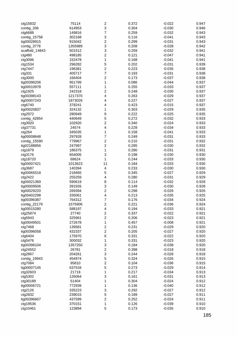
185
ctg15832 75114 2 0.372 -0.022 0.947
contig_336 614953 3 0.304 -0.030 0.946
ctg6688 149816 7 0.259 -0.032 0.943
contig_15758 302168 3 0.116 -0.041 0.943
tig00028915 915042 2 0.299 -0.031 0.943
contig_3778 1355989 3 0.208 -0.028 0.942
scaffold_14843 501512 3 0.259 -0.032 0.941
ctg480 498185 2 0.121 -0.047 0.941
ctg3096 152478 1 0.168 -0.041 0.941
ctg1534 296282 5 0.202 -0.031 0.939
ctg7447 196381 2 0.223 -0.035 0.938
ctg331 405717 7 0.193 -0.031 0.938
ctg3000 166404 2 0.173 -0.037 0.938
tig00396206 951799 1 0.086 -0.044 0.937
tig00010978 557111 1 0.255 -0.033 0.937
ctg1925 242318 2 0.248 -0.030 0.937
tig00398143 1217370 4 0.263 -0.029 0.937
tig00007243 1873026 4 0.227 -0.027 0.937
ctg6740 378241 4 0.423 -0.015 0.937
tig00020837 324132 1 0.303 -0.029 0.935
ctg2972 280949 9 0.222 -0.025 0.935
contig_42854 440649 5 0.272 -0.032 0.933
ctg3920 102920 2 0.340 -0.024 0.933
ctg37731 24574 4 0.228 -0.034 0.933
ctg264 345035 1 0.158 -0.041 0.933
tig00008648 297928 7 0.249 -0.031 0.933
contig_15590 779967 2 0.210 -0.031 0.932
tig02188856 247997 2 0.285 -0.030 0.932
ctg1879 186375 1 0.280 -0.031 0.931
ctg3176 654005 3 0.198 -0.030 0.930
ctg18720 68624 1 0.244 -0.033 0.930
tig00007421 1013623 11 0.184 -0.033 0.930
ctg3687 140394 4 0.233 -0.030 0.930
tig00065518 218465 5 0.345 -0.027 0.929
ctg2422 255259 4 0.280 -0.031 0.929
tig00021369 590619 8 0.114 -0.032 0.928
tig00009506 391926 3 0.149 -0.030 0.928
tig00029220 269394 2 0.298 -0.026 0.926
tig00402298 335061 4 0.213 -0.035 0.925
tig00396387 764312 7 0.176 -0.034 0.924
contig_22179 1575906 2 0.221 -0.036 0.924
tig00015280 588197 4 0.194 -0.033 0.921
ctg25874 27740 2 0.337 -0.022 0.921
ctg5943 325961 2 0.206 -0.023 0.921
tig00049501 272678 1 0.457 -0.008 0.921
ctg7468 139581 2 0.231 -0.029 0.920
tig00396058 432337 2 0.205 -0.027 0.920
ctg6404 175970 6 0.331 -0.022 0.920
ctg5476 300032 1 0.331 -0.023 0.920
tig00396104 1357250 3 0.184 -0.038 0.920
ctg24552 26781 2 0.398 -0.018 0.918
ctg2867 204261 3 0.244 -0.028 0.918
contig_19943 454974 5 0.324 -0.026 0.915
ctg7084 95810 2 0.104 -0.036 0.915
tig00007145 637534 5 0.273 -0.029 0.914
ctg32603 21718 1 0.217 -0.034 0.913
ctg5302 126064 3 0.161 -0.031 0.913
ctg30189 51404 1 0.304 -0.024 0.912
tig00006721 772939 1 0.136 -0.040 0.912
ctg2126 335223 3 0.292 -0.027 0.912
ctg2832 239015 5 0.189 -0.027 0.911
tig00396607 437599 2 0.252 -0.024 0.911
ctg19536 370151 1 0.126 -0.039 0.910
ctg10461 123894 5 0.173 -0.035 0.910

186
tig00014626 450713 6 0.418 -0.019 0.909
ctg2153 418519 3 0.200 -0.031 0.908
contig_42867 313187 1 0.195 -0.034 0.908
ctg1045 289974 2 0.080 -0.039 0.907
ctg11214 160364 1 0.329 -0.024 0.907
contig_66136 394579 3 0.257 -0.024 0.906
contig_8179 371295 2 0.215 -0.029 0.906
ctg828 395305 5 0.354 -0.027 0.905
tig00396437 1110687 6 0.264 -0.028 0.905
ctg2756 574959 4 0.292 -0.027 0.903
ctg8444 86154 1 0.225 -0.033 0.903
tig02169070 933255 2 0.369 -0.019 0.902
tig00021366 508188 8 0.190 -0.024 0.900
tig00017162 433066 3 0.195 -0.026 0.900
ctg5914 367944 2 0.181 -0.026 0.897
ctg9723 181896 8 0.378 -0.021 0.897
tig00026115 768126 4 0.195 -0.025 0.896
ctg20 636299 7 0.224 -0.025 0.896
ctg2825 159545 3 0.274 -0.019 0.895
tig00395824 471337 1 0.315 -0.021 0.895
tig00061405 200533 1 0.207 -0.033 0.895
ctg35065 19620 1 0.149 -0.037 0.894
ctg4659 237480 1 0.242 -0.030 0.894
contig_15994 1138584 4 0.193 -0.024 0.893
ctg2772 267361 3 0.155 -0.033 0.892
ctg11399 143120 4 0.104 -0.024 0.892
ctg376 1005629 3 0.289 -0.025 0.891
ctg5354 142662 9 0.265 -0.025 0.891
ctg17592 71530 4 0.148 -0.034 0.890
ctg1919 226599 1 0.377 -0.016 0.890
ctg15550 48275 1 0.210 -0.030 0.890
tig00000469 885151 4 0.321 -0.021 0.889
contig_13806 582359 2 0.209 -0.031 0.888
contig_21667 383255 3 0.169 -0.023 0.884
contig_11478 694499 5 0.229 -0.021 0.883
tig00397752 484912 5 0.177 -0.027 0.882
contig_41137 821796 1 0.119 -0.035 0.881
ctg513 294026 2 0.291 -0.019 0.881
tig00398012 450310 3 0.343 -0.021 0.880
tig00397729 700475 3 0.347 -0.019 0.880
contig_6272 456004 5 0.360 -0.021 0.878
tig00000373 623218 3 0.208 -0.027 0.876
contig_12923 1127836 3 0.157 -0.023 0.876
tig00401621 453680 11 0.132 -0.027 0.875
ctg14482 73888 1 0.239 -0.027 0.875
tig00396995 801080 7 0.341 -0.026 0.875
contig_2411 359992 3 0.418 -0.013 0.875
ctg9857 137557 1 0.358 -0.017 0.874
tig00004487 993603 10 0.290 -0.024 0.874
contig_11432 447392 7 0.217 -0.022 0.872
ctg22586 30770 1 0.173 -0.032 0.871
ctg12942 220129 1 0.097 -0.036 0.871
ctg12083 173781 3 0.174 -0.025 0.870
tig00010284 641476 4 0.194 -0.029 0.869
ctg1685 286088 2 0.207 -0.019 0.869
ctg18591 119419 2 0.334 -0.022 0.868
tig00018143 333515 10 0.278 -0.023 0.866
tig00006862 822413 9 0.280 -0.019 0.866
ctg868 376583 4 0.148 -0.029 0.866
contig_19797 905007 8 0.213 -0.021 0.865
tig00042400 328831 4 0.328 -0.022 0.864
tig00399924 745335 8 0.204 -0.020 0.863
ctg21874 87731 2 0.222 -0.026 0.862
ctg2508 503754 9 0.372 -0.017 0.860

187
ctg4501 323693 1 0.104 -0.031 0.859
tig00071454 302856 3 0.310 -0.022 0.859
tig00016676 577223 15 0.188 -0.019 0.859
ctg3401 196760 5 0.297 -0.023 0.858
tig02186571 405257 6 0.247 -0.019 0.856
tig00043155 690817 3 0.158 -0.026 0.855
ctg320 359004 2 0.315 -0.020 0.853
ctg2355 168242 3 0.169 -0.027 0.851
tig00009262 640215 1 0.340 -0.018 0.850
ctg972 331155 2 0.142 -0.022 0.849
tig00014641 600358 1 0.170 -0.022 0.848
tig00053395 255810 2 0.167 -0.023 0.848
ctg1804 188773 1 0.341 -0.016 0.847
tig00404812 420122 2 0.178 -0.028 0.846
tig00119373 254233 1 0.208 -0.027 0.845
ctg53790 9456 1 0.237 -0.025 0.845
tig00107002 695308 1 0.387 -0.013 0.841
contig_34695 361553 2 0.260 -0.024 0.840
ctg6552 221404 5 0.182 -0.024 0.840
ctg10579 127802 3 0.081 -0.031 0.837
contig_38800 584394 3 0.115 -0.027 0.835
ctg4700 122142 11 0.396 -0.017 0.835
ctg21 770111 1 0.332 -0.016 0.834
contig_49782 506649 6 0.173 -0.017 0.834
tig00395793 652341 1 0.112 -0.024 0.832
ctg3476 191175 3 0.232 -0.024 0.831
ctg2349 288377 9 0.348 -0.016 0.829
tig00001443 534525 6 0.246 -0.017 0.828
ctg11916 60490 4 0.187 -0.025 0.827
ctg43 734717 1 0.143 -0.028 0.826
ctg2260 278184 5 0.278 -0.020 0.825
tig00396873 456457 8 0.233 -0.023 0.825
ctg8957 120884 1 0.096 -0.030 0.824
ctg6985 176142 6 0.232 -0.021 0.822
tig02186482 686166 6 0.289 -0.018 0.822
ctg5425 540309 5 0.213 -0.014 0.818
ctg9560 77795 4 0.157 -0.021 0.816
tig02169355 936654 6 0.226 -0.017 0.814
ctg855 246009 1 0.211 -0.024 0.813
ctg47 624958 1 0.098 -0.028 0.812
contig_3405 962480 3 0.240 -0.014 0.811
tig00397350 237877 6 0.270 -0.016 0.811
ctg113 448522 5 0.220 -0.019 0.810
tig00002843 507905 1 0.302 -0.018 0.810
ctg15667 77389 1 0.166 -0.022 0.809
ctg9368 140361 2 0.291 -0.018 0.808
ctg1607 381967 1 0.332 -0.015 0.805
ctg26054 53731 2 0.193 -0.019 0.805
tig00086880 365570 2 0.179 -0.018 0.804
contig_17063 386425 8 0.318 -0.018 0.802
tig00028821 241823 4 0.162 -0.021 0.802
tig00398075 810072 11 0.185 -0.016 0.800
ctg6948 136897 5 0.389 -0.011 0.798
ctg893 591911 1 0.166 -0.023 0.797
ctg7615 202002 2 0.257 -0.019 0.795
ctg10661 121186 1 0.077 -0.026 0.793
tig00016413 430220 9 0.249 -0.020 0.792
tig00009368 611554 1 0.249 -0.019 0.791
ctg6122 146735 1 0.247 -0.019 0.791
ctg3010 285174 1 0.088 -0.023 0.790
ctg26702 27159 1 0.126 -0.025 0.789
contig_4080 959621 1 0.191 -0.023 0.788
ctg10736 116861 1 0.202 -0.020 0.788
ctg13002 87428 2 0.264 -0.019 0.788

188
tig00059861 627643 12 0.262 -0.016 0.788
ctg1189 223704 1 0.253 -0.019 0.786
ctg6643 116228 9 0.402 -0.014 0.784
ctg16873 61982 7 0.406 -0.014 0.783
contig_23935 405199 1 0.140 -0.023 0.783
scaffold_944 983878 5 0.280 -0.016 0.782
contig_24216 646077 1 0.303 -0.016 0.781
ctg666 461153 5 0.234 -0.016 0.777
tig02169060 484131 1 0.158 -0.023 0.777
ctg41660 15405 4 0.186 -0.019 0.777
tig02172068 929912 8 0.216 -0.016 0.776
contig_21672 317146 3 0.273 -0.018 0.773
ctg162 383129 3 0.242 -0.010 0.773
ctg3018 593326 6 0.265 -0.017 0.772
tig00401106 535082 4 0.301 -0.016 0.770
ctg3026 235553 3 0.243 -0.019 0.770
contig_12348 554702 1 0.268 -0.017 0.769
ctg17401 82555 2 0.172 -0.020 0.769
tig00399457 348368 10 0.310 -0.015 0.769
ctg12180 62582 8 0.260 -0.015 0.767
contig_8143 362708 8 0.261 -0.015 0.765
ctg9036 187932 1 0.230 -0.018 0.764
tig00026478 509051 10 0.215 -0.016 0.764
tig00396301 327657 1 0.181 -0.020 0.762
contig_27554 896793 5 0.232 -0.018 0.762
contig_23941 225916 3 0.233 -0.016 0.761
tig00395668 570316 1 0.164 -0.021 0.760
contig_1897 611172 5 0.456 -0.009 0.759
ctg55 494795 2 0.227 -0.012 0.757
tig00020570 411200 1 0.179 -0.020 0.756
ctg13348 99632 4 0.236 -0.016 0.755
contig_25226 268350 6 0.331 -0.014 0.755
ctg5331 116510 1 0.180 -0.019 0.755
ctg5245 116128 7 0.389 -0.012 0.755
tig00002219 811392 1 0.308 -0.014 0.753
tig00010983 525514 2 0.278 -0.010 0.753
ctg40423 16488 4 0.176 -0.015 0.753
ctg8715 79747 5 0.218 -0.018 0.752
ctg15909 121615 2 0.202 -0.017 0.752
ctg15398 48685 1 0.231 -0.017 0.751
ctg14134 53369 1 0.075 -0.016 0.751
ctg13926 124705 5 0.246 -0.017 0.750
tig02169085 314262 6 0.236 -0.016 0.749
ctg1101 225191 15 0.190 -0.015 0.749
tig02169753 492903 6 0.434 -0.008 0.745
ctg6079 104669 1 0.045 -0.023 0.744
tig00053246 529663 1 0.187 -0.018 0.744
contig_12366 351532 8 0.219 -0.013 0.741
ctg1496 443367 4 0.201 -0.015 0.741
ctg5337 192064 6 0.177 -0.018 0.740
ctg41 652889 4 0.391 -0.010 0.740
ctg19863 38670 1 0.139 -0.016 0.740
contig_46838 334555 7 0.302 -0.014 0.739
tig00023964 334911 1 0.123 -0.020 0.738
ctg14451 143494 3 0.222 -0.015 0.738
tig00020520 382633 1 0.136 -0.020 0.735
ctg1612 584733 9 0.308 -0.014 0.735
ctg137 546492 7 0.274 -0.014 0.735
tig00398152 581694 5 0.412 -0.009 0.733
tig00403695 556649 3 0.296 -0.013 0.733
ctg7444 91689 1 0.114 -0.021 0.731
contig_13693 1713974 5 0.178 -0.014 0.730
ctg20882 36235 5 0.365 -0.012 0.730
tig00404874 594238 1 0.337 -0.011 0.730

189
tig00396249 218342 4 0.327 -0.012 0.729
ctg126 608767 2 0.321 -0.012 0.728
ctg46793 12551 1 0.294 -0.013 0.727
tig02169302 611393 4 0.300 -0.013 0.727
tig00094389 335517 1 0.206 -0.017 0.727
ctg15640 59951 1 0.114 -0.017 0.726
tig00091870 717535 1 0.268 -0.014 0.726
contig_24646 285580 3 0.200 -0.013 0.726
contig_13429 1627540 2 0.295 -0.013 0.725
tig00003166 2916146 1 0.260 -0.013 0.725
contig_17367 313943 1 0.321 -0.012 0.723
contig_52794 588399 5 0.229 -0.015 0.722
ctg4434 124676 2 0.226 -0.015 0.722
tig00400896 322104 1 0.215 -0.014 0.721
contig_841 490440 3 0.312 -0.012 0.721
ctg5473 145183 2 0.196 -0.016 0.720
ctg8675 92129 2 0.329 -0.011 0.720
tig00396777 446511 3 0.177 -0.014 0.719
ctg7445 89986 8 0.283 -0.013 0.718
tig00066970 235126 2 0.237 -0.014 0.718
tig00046167 222597 2 0.355 -0.013 0.713
contig_13130 385754 2 0.191 -0.010 0.713
ctg9905 74857 5 0.278 -0.013 0.711
tig02173580 325920 5 0.426 -0.010 0.710
contig_7573 220342 5 0.397 -0.009 0.709
ctg11504 108138 3 0.283 -0.011 0.708
tig00004441 1175210 6 0.279 -0.010 0.707
ctg15821 262696 10 0.296 -0.011 0.705
ctg10240 72657 4 0.232 -0.014 0.705
ctg4903 204066 1 0.251 -0.013 0.705
contig_10092 1119842 2 0.226 -0.009 0.704
ctg5756 218058 2 0.379 -0.009 0.704
ctg1490 490974 8 0.359 -0.010 0.704
contig_21119 661486 3 0.157 -0.014 0.703
tig00006792 266482 4 0.242 -0.014 0.703
tig00043771 1360784 7 0.187 -0.008 0.703
ctg7316 223284 6 0.400 -0.008 0.702
tig00403580 1746765 4 0.406 -0.008 0.700
contig_18859 1197349 2 0.216 -0.014 0.700
ctg63536 4982 1 0.111 -0.014 0.700
ctg26069 27437 11 0.157 -0.012 0.699
tig00030047 269674 3 0.268 -0.011 0.699
ctg8412 84657 4 0.300 -0.012 0.698
ctg33226 42254 1 0.202 -0.014 0.695
tig00036500 465936 9 0.284 -0.010 0.695
tig02170401 297736 8 0.315 -0.011 0.694
tig00009173 539588 1 0.148 -0.014 0.694
contig_48038 281645 5 0.103 -0.013 0.693
tig00043883 220572 1 0.359 -0.008 0.692
ctg2865 273214 1 0.089 -0.017 0.692
tig00073367 813981 12 0.262 -0.010 0.692
ctg16876 43751 7 0.242 -0.012 0.691
ctg5630 133340 1 0.174 -0.013 0.688
tig00397346 502732 2 0.251 -0.013 0.688
tig00055575 1103812 6 0.160 -0.009 0.688
tig00041928 973234 10 0.263 -0.011 0.687
ctg930 522006 4 0.364 -0.009 0.687
scaffold_16094 302431 4 0.205 -0.009 0.686
ctg16917 108112 1 0.255 -0.011 0.685
ctg13904 101038 2 0.271 -0.011 0.682
tig00396056 789257 2 0.337 -0.009 0.680
ctg325 760294 2 0.186 -0.012 0.677
ctg1202 623912 2 0.273 -0.009 0.677
tig00027453 527258 2 0.200 -0.010 0.674

190
ctg10529 216459 1 0.229 -0.012 0.673
tig00395581 211649 1 0.166 -0.013 0.671
ctg698 290216 7 0.342 -0.009 0.670
tig00397222 228681 1 0.184 -0.012 0.667
ctg7267 91819 2 0.105 -0.012 0.667
tig00396525 704356 2 0.113 -0.012 0.666
ctg10284 71050 1 0.379 -0.007 0.665
ctg3968 268251 1 0.195 -0.013 0.664
ctg9253 78260 4 0.081 -0.012 0.662
ctg6432 103239 1 0.192 -0.012 0.658
tig00083019 730520 18 0.268 -0.009 0.657
ctg570 385748 4 0.237 -0.011 0.656
ctg919 692053 3 0.327 -0.008 0.656
ctg6764 164637 1 0.174 -0.012 0.655
contig_3490 322447 3 0.319 -0.009 0.654
ctg3438 403988 1 0.110 -0.011 0.652
ctg21369 35982 3 0.382 -0.006 0.652
contig_8493 511816 7 0.235 -0.009 0.651
ctg24876 28312 2 0.124 -0.011 0.648
ctg500 345663 2 0.355 -0.008 0.646
tig00000780 278461 1 0.256 -0.009 0.646
ctg5116 168283 4 0.367 -0.008 0.646
contig_16273 663146 1 0.064 -0.012 0.645
tig02172889 252454 9 0.199 -0.008 0.645
ctg18922 75457 1 0.247 -0.009 0.644
ctg1530 577320 1 0.288 -0.009 0.644
ctg1387 514557 1 0.208 -0.010 0.643
ctg4567 191649 2 0.420 -0.005 0.643
contig_5195 843944 4 0.232 -0.009 0.641
contig_897 455080 2 0.276 -0.009 0.640
ctg805 604068 5 0.307 -0.008 0.639
tig00010893 1338994 15 0.302 -0.007 0.636
tig02171490 1030388 8 0.229 -0.008 0.636
ctg31238 34468 5 0.377 -0.006 0.635
ctg35899 19864 1 0.362 -0.006 0.634
tig00395320 1033643 6 0.367 -0.007 0.632
tig00028901 551257 2 0.236 -0.009 0.631
ctg8565 121928 5 0.283 -0.008 0.631
ctg3267 370137 8 0.317 -0.007 0.630
tig00399725 355106 1 0.314 -0.007 0.630
ctg8991 210350 8 0.441 -0.005 0.629
ctg8008 104172 2 0.250 -0.008 0.628
ctg43878 14345 2 0.304 -0.007 0.628
tig00400853 386323 3 0.119 -0.008 0.627
contig_33969 263993 8 0.292 -0.008 0.627
ctg2908 226314 9 0.266 -0.007 0.627
tig00014977 370639 1 0.271 -0.008 0.626
tig00017255 471635 1 0.086 -0.009 0.626
scaffold_41143 467631 2 0.144 -0.008 0.624
ctg25649 57345 2 0.226 -0.007 0.623
ctg4797 224255 2 0.247 -0.008 0.620
contig_31783 244048 2 0.076 -0.007 0.618
ctg19669 82762 1 0.345 -0.007 0.615
contig_43563 439607 4 0.228 -0.007 0.614
ctg1059 573554 1 0.215 -0.008 0.614
ctg12213 62309 1 0.335 -0.005 0.613
ctg182 397717 6 0.454 -0.004 0.613
tig00040415 1244426 14 0.242 -0.005 0.611
ctg1497 260225 3 0.318 -0.007 0.611
tig00038427 437035 2 0.176 -0.009 0.611
ctg6661 141709 4 0.255 -0.007 0.611
ctg2241 250175 2 0.194 -0.008 0.610
contig_40725 709630 1 0.148 -0.008 0.608
ctg4266 119268 7 0.411 -0.004 0.608

191
ctg1381 234532 1 0.197 -0.009 0.607
contig_5714 681477 1 0.275 -0.007 0.607
ctg8256 87012 1 0.072 -0.008 0.606
tig00395532 669779 8 0.253 -0.006 0.606
tig00042780 306102 9 0.357 -0.005 0.604
ctg6808 258490 13 0.180 -0.005 0.600
contig_6104 500458 10 0.219 -0.007 0.599
ctg2529 433038 7 0.279 -0.005 0.597
tig00001967 1524795 2 0.285 -0.006 0.595
contig_17921 524413 2 0.244 -0.007 0.594
ctg16252 45673 9 0.317 -0.006 0.592
ctg3934 547533 1 0.167 -0.006 0.591
tig00395527 1034874 1 0.322 -0.006 0.591
tig00035074 512272 9 0.329 -0.005 0.590
contig_13836 783511 2 0.228 -0.007 0.590
tig02188898 666550 3 0.137 -0.006 0.589
ctg5527 184576 4 0.253 -0.006 0.588
tig00399081 1078544 1 0.184 -0.007 0.587
ctg1912 487146 6 0.236 -0.004 0.587
tig00400810 487621 1 0.202 -0.007 0.586
tig00053577 244843 1 0.141 -0.007 0.585
ctg4235 910052 3 0.257 -0.006 0.585
tig00027697 488684 11 0.337 -0.005 0.583
ctg15102 165018 4 0.162 -0.005 0.582
contig_46319 441250 4 0.271 -0.006 0.581
tig00401160 431609 3 0.271 -0.006 0.579
ctg11032 228265 2 0.185 -0.007 0.578
ctg1334 216750 1 0.215 -0.006 0.576
tig02169171 1137723 5 0.243 -0.005 0.575
ctg8648 245069 2 0.246 -0.006 0.575
tig00007716 1298565 1 0.053 -0.007 0.574
tig00397782 1052995 2 0.437 -0.003 0.573
tig00047187 221709 9 0.318 -0.005 0.571
ctg1936 284549 1 0.109 -0.006 0.570
tig00400104 303083 1 0.053 -0.007 0.570
ctg35355 18397 2 0.178 -0.004 0.569
ctg8024 110807 4 0.218 -0.005 0.568
tig00398510 391527 5 0.295 -0.005 0.568
contig_1845 734391 3 0.239 -0.004 0.567
tig02170273 603096 10 0.231 -0.004 0.566
ctg11810 63609 2 0.207 -0.004 0.564
contig_12211 409191 6 0.171 -0.004 0.562
tig00004124 1011600 8 0.259 -0.003 0.561
ctg6956 277633 1 0.202 -0.005 0.561
tig00041919 508276 1 0.284 -0.004 0.557
ctg1263 425904 3 0.193 -0.004 0.556
tig02170092 629326 1 0.088 -0.005 0.556
tig00036475 647372 4 0.235 -0.004 0.555
ctg2119 189271 4 0.256 -0.004 0.555
ctg831 389348 15 0.229 -0.004 0.555
tig00018277 587778 1 0.287 -0.004 0.555
tig00399333 496237 9 0.267 -0.004 0.555
tig02171434 533159 2 0.188 -0.005 0.555
contig_34639 546659 2 0.155 -0.004 0.549
ctg17345 42194 3 0.250 -0.004 0.547
ctg1748 263778 6 0.305 -0.004 0.547
ctg1061 359285 2 0.212 -0.004 0.546
ctg2655 399946 2 0.239 -0.004 0.545
ctg5625 210968 2 0.217 -0.003 0.545
tig00076252 521038 1 0.216 -0.004 0.543
tig00006648 777613 6 0.278 -0.003 0.542
tig00023974 948520 1 0.107 -0.004 0.542
contig_1864 239348 9 0.237 -0.004 0.540
ctg838 507887 1 0.117 -0.004 0.540

192
ctg313 401801 4 0.297 -0.003 0.538
tig00015391 506855 1 0.303 -0.003 0.537
tig00102205 1311232 2 0.389 -0.003 0.537
tig00400191 279898 2 0.187 -0.002 0.533
tig00019828 437531 1 0.225 -0.003 0.533
tig00396412 1132115 1 0.351 -0.003 0.533
tig02172912 349288 1 0.216 -0.003 0.531
contig_50564 508870 2 0.046 -0.004 0.530
tig00402541 1116159 6 0.208 -0.003 0.529
ctg3507 799998 3 0.156 -0.003 0.529
tig00014687 531722 3 0.269 -0.002 0.529
ctg2158 928513 5 0.375 -0.002 0.528
ctg19070 39069 1 0.193 -0.003 0.525
ctg14829 102996 5 0.285 -0.002 0.525
scaffold_62778 301450 1 0.309 -0.003 0.524
ctg111 550433 3 0.425 -0.002 0.523
tig00001521 1814178 8 0.209 -0.002 0.523
tig00397854 1340822 6 0.257 -0.002 0.523
ctg16812 52416 1 0.293 -0.002 0.520
tig00040162 655590 2 0.130 -0.003 0.520
contig_38988 427185 4 0.295 -0.002 0.519
tig00397426 224590 4 0.295 -0.002 0.518
ctg16789 81665 5 0.155 -0.002 0.516
ctg27966 26012 6 0.257 -0.002 0.516
tig00399224 274976 7 0.180 -0.002 0.514
contig_167 379846 5 0.229 -0.002 0.513
tig00402753 297647 7 0.205 -0.002 0.512
ctg18611 40214 3 0.204 -0.001 0.512
tig00009696 621637 1 0.163 -0.002 0.511
tig00020401 361343 1 0.237 -0.002 0.510
ctg6939 264968 1 0.206 -0.002 0.510
tig00008084 992601 3 0.391 -0.002 0.509
tig00008190 629190 1 0.092 -0.002 0.508
tig02171222 219427 7 0.304 -0.001 0.508
ctg2366 480735 7 0.337 -0.001 0.506
tig00399004 340133 1 0.210 -0.001 0.506
contig_30102 390755 1 0.062 -0.002 0.506
ctg51138 10694 1 0.165 -0.001 0.505
tig00014974 549881 1 0.310 -0.002 0.505
ctg5389 240228 1 0.337 -0.002 0.503
tig00398942 533835 6 0.239 -0.001 0.503
contig_34666 642048 2 0.305 -0.002 0.502
tig00396028 570496 1 0.241 -0.002 0.502
ctg11215 66374 1 0.077 -0.001 0.502
contig_24015 410659 1 0.188 -0.001 0.501
contig_38459 326343 1 0.184 -0.001 0.500
ctg1899 309002 4 0.226 -0.001 0.500
ctg17228 43623 1 0.247 -0.001 0.498
ctg32 723123 1 0.285 -0.002 0.498
ctg53500 9450 1 0.267 -0.001 0.494
tig00003469 331209 1 0.292 -0.001 0.493
ctg7102 96382 1 0.275 -0.001 0.493
scaffold_34793 251364 3 0.210 -0.001 0.492
contig_24247 834838 2 0.283 -0.001 0.490
tig00014020 484590 1 0.119 0.000 0.490
ctg8146 216194 1 0.200 0.000 0.489
contig_10102 552091 1 0.194 0.000 0.489
ctg26463 27064 1 0.144 0.000 0.488
tig00031805 320586 1 0.275 -0.001 0.487
tig00006081 1034151 3 0.178 0.000 0.486
tig00016527 794251 2 0.249 0.000 0.482
tig02168946 650385 2 0.336 0.000 0.482
tig02186709 609292 3 0.269 0.000 0.482
tig00077938 256834 1 0.269 0.000 0.481

193
ctg9566 314685 7 0.200 0.000 0.479
ctg5785 214093 1 0.252 0.000 0.475
tig00044630 922835 3 0.315 0.000 0.474
tig00399904 430432 10 0.270 0.001 0.474
tig00019804 373618 6 0.331 0.001 0.473
ctg3152 733178 10 0.306 0.001 0.471
tig02170015 398876 4 0.236 0.000 0.469
tig00032843 353947 2 0.298 0.000 0.468
ctg5867 219649 1 0.244 0.001 0.468
contig_9662 1228451 10 0.280 0.001 0.467
tig02169631 837755 5 0.200 0.001 0.465
ctg616 527122 5 0.203 0.001 0.464
ctg1791 298529 4 0.275 0.000 0.464
tig00034802 480886 8 0.327 0.001 0.462
ctg2400 344491 1 0.098 0.002 0.462
ctg10561 117120 6 0.141 0.001 0.462
tig00030658 331077 7 0.224 0.001 0.459
tig00023902 543692 3 0.196 0.001 0.457
contig_9558 882490 1 0.118 0.002 0.457
ctg18061 41478 2 0.313 0.001 0.456
tig00396080 408416 8 0.272 0.001 0.455
ctg3832 337311 2 0.161 0.002 0.454
tig00061516 328044 4 0.260 0.001 0.454
ctg19368 37938 8 0.257 0.001 0.454
ctg7556 83281 1 0.059 0.002 0.453
tig00399854 715880 5 0.131 0.001 0.453
contig_9324 1484920 1 0.281 0.001 0.453
ctg1080 345086 3 0.318 0.002 0.453
tig00399158 566761 3 0.275 0.001 0.452
tig00399063 297754 6 0.239 0.002 0.452
ctg2267 287725 3 0.196 0.002 0.452
tig00038898 203416 1 0.057 0.003 0.452
contig_35763 924599 4 0.161 0.002 0.451
contig_55226 469688 2 0.184 0.002 0.451
ctg1391 542348 3 0.382 0.001 0.450
contig_5364 441384 2 0.143 0.001 0.449
contig_11399 872055 6 0.213 0.002 0.449
ctg3925 129008 7 0.274 0.002 0.446
ctg4594 121809 2 0.240 0.002 0.445
scaffold_68823 749868 3 0.227 0.002 0.443
ctg22063 44424 3 0.083 0.003 0.443
ctg25088 60155 1 0.135 0.003 0.443
ctg3847 140969 1 0.037 0.004 0.443
ctg4936 118375 2 0.150 0.002 0.441
ctg2463 300679 2 0.327 0.002 0.440
contig_18092 623818 2 0.258 0.002 0.440
ctg16750 92128 4 0.182 0.002 0.440
tig02186728 403509 3 0.155 0.003 0.439
contig_405 661065 3 0.209 0.002 0.438
tig00027581 444229 4 0.294 0.002 0.437
scaffold_6949 368580 3 0.342 0.002 0.437
tig00402141 287753 1 0.197 0.003 0.435
contig_17666 849625 14 0.292 0.002 0.435
tig00027224 341833 1 0.207 0.003 0.434
contig_4310 359971 3 0.184 0.003 0.434
contig_70356 503602 1 0.313 0.002 0.434
ctg3294 391014 3 0.321 0.002 0.434
ctg2316 208433 1 0.257 0.003 0.433
tig00399036 399234 1 0.187 0.004 0.433
tig00397290 1137711 2 0.115 0.003 0.432
ctg6707 98833 2 0.234 0.003 0.431
ctg19766 36126 3 0.189 0.003 0.430
tig00003060 473357 4 0.171 0.003 0.429
contig_16508 284442 2 0.159 0.004 0.428

194
contig_1664 360730 5 0.375 0.003 0.428
ctg4071 383765 1 0.394 0.001 0.428
ctg3996 138028 5 0.321 0.003 0.427
ctg11442 65828 1 0.305 0.002 0.427
ctg26023 28036 12 0.342 0.002 0.426
tig00409871 202717 1 0.115 0.003 0.425
ctg8856 124036 1 0.109 0.005 0.423
tig00085471 646292 6 0.306 0.003 0.423
ctg8695 83338 1 0.249 0.004 0.423
contig_27873 199960 5 0.270 0.003 0.422
ctg2286 329912 5 0.180 0.003 0.421
contig_48726 493185 3 0.199 0.002 0.421
ctg11764 63857 8 0.186 0.002 0.420
ctg1397 396155 1 0.317 0.003 0.420
ctg5410 128609 1 0.111 0.004 0.420
ctg6133 147616 2 0.205 0.003 0.419
ctg28915 23102 1 0.167 0.005 0.419
ctg5922 107431 1 0.233 0.003 0.418
tig00042959 303547 1 0.339 0.002 0.417
ctg9169 139841 2 0.319 0.003 0.416
tig00045243 465416 11 0.253 0.005 0.415
ctg7079 95697 6 0.303 0.004 0.411
ctg174 431346 4 0.190 0.004 0.409
tig02170991 444866 5 0.229 0.004 0.409
contig_52009 666542 2 0.333 0.003 0.409
contig_55590 388109 1 0.210 0.005 0.407
ctg2627 297983 2 0.155 0.006 0.407
tig00024900 301345 5 0.253 0.004 0.407
contig_16859 753330 4 0.329 0.004 0.407
ctg479 1027179 1 0.285 0.004 0.405
tig00039289 422826 4 0.327 0.003 0.405
ctg3397 135310 3 0.216 0.003 0.405
tig00038294 302025 6 0.114 0.004 0.405
contig_8775 285451 1 0.137 0.006 0.403
contig_27594 1956444 4 0.214 0.004 0.403
ctg11895 92023 3 0.153 0.005 0.403
tig00002241 860234 2 0.220 0.006 0.403
ctg238 498939 2 0.200 0.005 0.402
contig_29523 221790 1 0.334 0.004 0.402
tig00043906 1233451 4 0.253 0.004 0.401
tig00395980 590998 6 0.346 0.003 0.401
tig02169307 295274 3 0.129 0.006 0.401
tig00026057 346620 1 0.116 0.007 0.399
ctg11792 80376 2 0.261 0.004 0.398
ctg11173 389268 1 0.287 0.004 0.398
contig_10636 230810 2 0.379 0.003 0.397
ctg1333 1139614 5 0.173 0.005 0.396
contig_1486 1077882 9 0.179 0.004 0.395
tig00397833 1018425 2 0.270 0.005 0.394
tig02186434 524742 1 0.168 0.006 0.393
tig00402945 237922 3 0.318 0.004 0.391
scaffold_45183 233345 8 0.266 0.005 0.390
contig_49703 241010 1 0.275 0.005 0.389
ctg11542 64574 1 0.247 0.005 0.389
scaffold_64729 624955 1 0.252 0.005 0.388
tig00399346 1028168 3 0.194 0.006 0.387
ctg2938 352946 3 0.363 0.003 0.387
ctg35727 18729 2 0.227 0.005 0.385
contig_16955 522175 3 0.167 0.007 0.385
ctg6821 98412 5 0.285 0.005 0.385
ctg30127 23394 6 0.270 0.006 0.384
ctg23252 88985 2 0.411 0.002 0.382
ctg23626 51948 3 0.277 0.005 0.381
tig00403819 607026 14 0.238 0.005 0.381

195
ctg11033 68333 1 0.244 0.006 0.381
tig00031425 691299 16 0.325 0.005 0.380
tig00064960 478952 5 0.304 0.005 0.379
ctg39807 16525 4 0.218 0.006 0.378
ctg16510 45327 1 0.130 0.007 0.378
ctg366 614486 3 0.159 0.006 0.376
ctg9334 264644 1 0.054 0.009 0.375
ctg388 517509 4 0.181 0.006 0.374
ctg17374 72477 2 0.077 0.007 0.372
ctg1518 300125 1 0.177 0.009 0.370
contig_28127 464494 1 0.366 0.004 0.368
tig00399293 499527 12 0.266 0.006 0.365
ctg4364 313481 2 0.265 0.007 0.363
contig_7963 283313 6 0.186 0.008 0.363
ctg7839 326469 3 0.281 0.007 0.361
tig00011099 903735 4 0.356 0.006 0.361
ctg11226 406031 2 0.228 0.008 0.361
contig_11332 693295 1 0.120 0.009 0.359
ctg1241 556466 2 0.454 0.001 0.359
ctg10413 74261 3 0.236 0.007 0.358
contig_3519 723942 7 0.311 0.005 0.358
ctg10371 221668 9 0.368 0.006 0.357
tig00049519 502421 5 0.270 0.007 0.357
ctg3647 334639 4 0.208 0.008 0.357
contig_16291 215563 3 0.230 0.007 0.356
tig00396472 1300381 6 0.221 0.006 0.355
ctg792 256016 2 0.280 0.006 0.355
contig_11612 514562 1 0.123 0.011 0.354
ctg50750 26482 11 0.164 0.006 0.353
tig00000220 1112024 4 0.284 0.006 0.351
contig_26538 225584 5 0.273 0.006 0.349
ctg3241 433825 2 0.109 0.009 0.349
tig00008767 823990 10 0.291 0.006 0.348
ctg21642 31698 4 0.309 0.007 0.346
ctg3161 562706 1 0.122 0.009 0.346
ctg2376 405901 11 0.216 0.007 0.345
ctg3232 583900 3 0.226 0.008 0.344
tig00397077 323985 12 0.190 0.006 0.344
tig00061909 406925 1 0.196 0.010 0.342
tig00042694 313962 2 0.184 0.010 0.342
tig00017426 722482 5 0.293 0.007 0.341
ctg713 278249 4 0.162 0.008 0.341
contig_24117 377481 1 0.176 0.010 0.341
tig00004882 305917 7 0.271 0.008 0.340
ctg24806 28923 3 0.082 0.011 0.339
tig00045603 1505374 10 0.227 0.009 0.339
ctg4373 128964 3 0.287 0.008 0.338
tig00011884 1225809 12 0.201 0.007 0.338
ctg2395 404071 2 0.265 0.009 0.337
tig00002394 2038556 2 0.153 0.012 0.337
ctg2044 489276 1 0.246 0.009 0.337
ctg2809 187657 1 0.146 0.011 0.337
ctg450 299471 7 0.401 0.006 0.337
ctg2273 177579 2 0.127 0.010 0.336
contig_8265 226666 5 0.366 0.006 0.334
ctg11118 100228 2 0.080 0.010 0.334
tig00397604 528125 6 0.297 0.009 0.333
tig00398120 245272 3 0.267 0.006 0.333
ctg5105 307454 2 0.049 0.011 0.332
tig00045694 580614 4 0.321 0.007 0.330
tig00029766 895646 4 0.246 0.008 0.330
ctg883 647412 3 0.102 0.011 0.329
ctg712 302024 4 0.322 0.008 0.329
ctg183 759955 8 0.275 0.009 0.329

196
ctg1920 666823 11 0.306 0.008 0.329
tig00011506 783833 3 0.128 0.012 0.328
ctg6988 97337 4 0.211 0.010 0.328
contig_47429 246707 2 0.123 0.008 0.327
tig00099272 527006 3 0.332 0.007 0.326
tig00011771 645681 2 0.246 0.010 0.325
ctg1529 420124 8 0.359 0.006 0.325
ctg5497 203990 1 0.109 0.014 0.324
ctg21508 62935 3 0.129 0.012 0.323
tig00003558 705364 3 0.252 0.006 0.323
tig02169097 318812 1 0.234 0.009 0.323
contig_3679 252125 1 0.111 0.014 0.322
contig_34045 1449546 1 0.141 0.013 0.322
ctg3846 305419 2 0.276 0.008 0.321
ctg11944 114540 6 0.335 0.009 0.320
ctg5397 111370 1 0.292 0.009 0.319
ctg21811 69469 14 0.271 0.009 0.318
ctg5832 158175 2 0.084 0.013 0.316
tig00008230 1400285 4 0.259 0.010 0.316
contig_12673 479480 10 0.369 0.007 0.316
ctg17209 43325 3 0.249 0.009 0.315
contig_26028 448753 1 0.217 0.012 0.315
tig00030298 243623 6 0.110 0.010 0.315
tig02170901 829001 5 0.237 0.009 0.313
ctg19165 47385 2 0.354 0.006 0.311
ctg12719 60178 3 0.286 0.010 0.309
tig00027603 286992 4 0.435 0.005 0.308
ctg54 641522 2 0.260 0.008 0.308
tig00082947 362372 4 0.213 0.012 0.308
contig_5161 1115787 5 0.243 0.009 0.307
ctg1371 344290 1 0.172 0.013 0.307
tig00395483 847536 2 0.152 0.011 0.307
tig00050415 277569 6 0.123 0.009 0.306
contig_10263 505274 3 0.236 0.008 0.306
tig00003355 271986 1 0.152 0.013 0.304
ctg9546 81194 5 0.266 0.011 0.304
tig00403306 291777 2 0.403 0.005 0.302
ctg15403 67458 2 0.225 0.011 0.302
tig02171032 898652 8 0.154 0.010 0.301
tig00398109 263642 5 0.313 0.009 0.301
tig00397477 419834 4 0.152 0.012 0.300
tig00396306 735482 12 0.166 0.012 0.299
tig00405137 269972 5 0.382 0.007 0.298
contig_69386 378855 1 0.359 0.007 0.297
ctg5375 200329 3 0.192 0.012 0.297
scaffold_26714 221214 1 0.327 0.010 0.296
tig02173403 539115 3 0.401 0.007 0.295
ctg2179 338079 2 0.193 0.011 0.295
tig00002471 718824 3 0.230 0.013 0.294
contig_1209 476419 2 0.330 0.009 0.293
ctg1668 321688 12 0.335 0.009 0.293
ctg1967 178723 10 0.218 0.010 0.292
contig_26950 996727 3 0.344 0.008 0.292
ctg1809 1047252 2 0.163 0.014 0.291
ctg2274 195032 2 0.309 0.010 0.290
tig00402136 368560 3 0.295 0.010 0.290
tig00060131 617991 6 0.325 0.010 0.290
tig00396701 410243 4 0.243 0.011 0.290
ctg8567 83098 3 0.184 0.011 0.287
ctg4670 199821 1 0.169 0.015 0.286
ctg16687 60298 1 0.136 0.017 0.285
ctg386 578986 3 0.296 0.011 0.284
tig00005188 869273 2 0.182 0.014 0.282
contig_50820 223879 2 0.308 0.011 0.281

197
tig00011756 1256973 1 0.308 0.011 0.281
tig00022871 832104 4 0.160 0.016 0.280
contig_26333 3510238 20 0.234 0.011 0.280
ctg59 461472 1 0.175 0.015 0.279
ctg48563 12119 3 0.328 0.010 0.279
scaffold_5606 863916 1 0.165 0.014 0.278
tig00031524 621365 16 0.369 0.010 0.276
ctg8119 176077 2 0.196 0.014 0.276
tig02186286 784776 3 0.109 0.012 0.276
contig_29836 269249 3 0.206 0.015 0.276
ctg22323 60152 1 0.365 0.008 0.275
ctg2509 192930 7 0.139 0.013 0.273
tig02186979 276463 3 0.355 0.007 0.272
ctg755 377340 5 0.336 0.010 0.272
ctg3033 172190 5 0.238 0.013 0.271
ctg1023 251366 2 0.190 0.012 0.270
tig00021227 391113 14 0.201 0.013 0.269
ctg9372 140531 2 0.217 0.015 0.269
ctg946 261740 1 0.334 0.010 0.268
tig00060048 455239 3 0.164 0.016 0.268
ctg9658 429156 1 0.162 0.015 0.266
tig00034225 431080 1 0.281 0.012 0.266
ctg1143 269436 16 0.374 0.011 0.265
ctg13353 64487 2 0.219 0.015 0.263
ctg4676 655169 1 0.168 0.017 0.263
ctg1175 1488075 10 0.223 0.012 0.263
tig00396252 2234354 4 0.212 0.011 0.263
contig_16422 412391 9 0.271 0.012 0.262
ctg12304 99606 1 0.394 0.006 0.262
ctg41048 16536 1 0.367 0.008 0.262
ctg1950 226520 2 0.104 0.018 0.260
contig_8502 659955 3 0.311 0.012 0.259
tig00104814 1793396 4 0.232 0.014 0.259
tig00025127 537042 4 0.321 0.012 0.259
ctg194 600697 4 0.199 0.013 0.258
ctg6063 225047 2 0.293 0.007 0.258
tig00044057 466073 1 0.247 0.015 0.257
tig00395942 338607 1 0.315 0.012 0.257
ctg752 602464 4 0.404 0.006 0.255
ctg34789 17479 3 0.258 0.015 0.254
tig02170971 414449 6 0.338 0.008 0.254
ctg3 1179550 12 0.201 0.014 0.254
tig00001022 1086513 8 0.200 0.015 0.253
ctg415 311524 1 0.216 0.016 0.253
ctg8985 210385 1 0.088 0.020 0.252
contig_2258 313162 3 0.321 0.011 0.252
ctg4939 265483 1 0.133 0.020 0.252
tig00004411 978213 11 0.348 0.014 0.252
ctg23705 43644 4 0.159 0.014 0.252
contig_59892 425997 4 0.162 0.017 0.251
tig00399998 282483 1 0.121 0.018 0.251
ctg15020 55150 1 0.179 0.015 0.250
ctg50003 20875 2 0.149 0.015 0.249
contig_27618 278105 2 0.146 0.017 0.249
tig00053685 529554 8 0.240 0.013 0.249
ctg177 471256 2 0.272 0.015 0.249
tig00397775 602392 6 0.181 0.012 0.248
ctg3365 406722 5 0.239 0.016 0.248
ctg9125 76434 2 0.130 0.013 0.247
ctg4715 460241 6 0.229 0.015 0.246
tig00395493 735867 3 0.196 0.016 0.246
tig00397358 211492 2 0.182 0.013 0.246
ctg1157 328581 1 0.196 0.016 0.245
ctg17303 40441 1 0.343 0.011 0.245

198
ctg6668 100423 4 0.137 0.020 0.245
ctg7718 88837 3 0.248 0.015 0.244
ctg6837 427499 5 0.275 0.016 0.244
tig00052855 768200 1 0.237 0.016 0.244
ctg38 1002682 1 0.231 0.016 0.243
tig02186981 429664 1 0.253 0.014 0.242
contig_11800 293398 4 0.279 0.011 0.242
ctg26085 41784 2 0.226 0.018 0.241
tig00398125 242286 3 0.286 0.015 0.239
scaffold_4683 835377 8 0.299 0.014 0.239
tig00019413 834945 1 0.305 0.014 0.238
tig00395664 739937 1 0.374 0.009 0.237
ctg4981 238808 5 0.323 0.014 0.236
ctg10095 116421 1 0.106 0.022 0.235
ctg6562 100056 6 0.441 0.011 0.235
contig_700 528404 10 0.220 0.015 0.234
ctg4863 119947 3 0.127 0.018 0.234
ctg1475 293470 1 0.355 0.009 0.233
contig_28122 981579 3 0.305 0.016 0.233
ctg18773 38018 11 0.086 0.016 0.232
tig02170329 932701 1 0.173 0.019 0.232
contig_9938 210024 2 0.325 0.013 0.230
contig_28334 417081 3 0.190 0.020 0.230
ctg6202 106203 1 0.257 0.016 0.229
ctg7818 171048 5 0.270 0.012 0.228
ctg22944 32023 2 0.196 0.019 0.228
tig00027088 326734 1 0.214 0.019 0.227
ctg3204 256046 3 0.276 0.018 0.227
ctg13400 51769 2 0.339 0.013 0.226
ctg607 520191 2 0.349 0.012 0.226
tig00396649 1110334 6 0.248 0.015 0.226
ctg19555 38077 6 0.248 0.016 0.226
ctg10144 130904 9 0.188 0.018 0.225
ctg13430 177202 1 0.350 0.012 0.224
ctg2815 148288 3 0.232 0.015 0.223
ctg46 597493 4 0.274 0.015 0.222
ctg505 732007 2 0.316 0.014 0.222
tig00032134 632509 1 0.225 0.018 0.221
tig00034708 906525 5 0.273 0.014 0.220
tig00083023 456639 1 0.185 0.021 0.219
tig00014463 384586 8 0.313 0.015 0.219
ctg812 258346 3 0.392 0.011 0.218
contig_30589 301511 3 0.190 0.018 0.218
ctg2384 234273 2 0.216 0.019 0.218
ctg4951 130550 1 0.313 0.013 0.216
ctg501 324510 1 0.242 0.018 0.215
contig_49819 327541 2 0.140 0.023 0.214
tig00395565 484104 2 0.103 0.021 0.214
ctg791 410033 2 0.311 0.015 0.214
tig00398853 541814 2 0.219 0.019 0.214
contig_4852 367073 1 0.320 0.012 0.214
ctg5333 174133 2 0.407 0.010 0.214
ctg24568 81426 1 0.266 0.017 0.213
ctg1298 491818 3 0.221 0.020 0.213
ctg5899 178746 6 0.192 0.018 0.213
ctg5912 109367 3 0.149 0.022 0.213
ctg10292 137413 7 0.371 0.013 0.213
tig00396717 1067560 2 0.256 0.012 0.212
ctg22309 32068 1 0.261 0.018 0.212
contig_27424 766992 2 0.191 0.022 0.212
ctg9604 129815 2 0.304 0.013 0.212
contig_6376 506229 18 0.311 0.016 0.209
ctg7623 319599 2 0.183 0.015 0.209
tig00031330 337571 4 0.267 0.018 0.208

199
tig00395829 939538 1 0.085 0.025 0.207
ctg4442 128076 1 0.199 0.022 0.207
contig_14639 342501 1 0.237 0.020 0.206
ctg12753 107548 5 0.246 0.019 0.206
ctg4226 130450 2 0.319 0.014 0.205
tig00016242 349565 3 0.333 0.015 0.205
ctg19 1757703 1 0.279 0.010 0.205
contig_40126 220821 6 0.401 0.012 0.204
ctg5199 117210 5 0.311 0.016 0.204
ctg1363 310217 2 0.298 0.017 0.203
tig00009046 363448 4 0.288 0.017 0.203
contig_34921 726249 1 0.171 0.023 0.202
tig02173057 245732 10 0.274 0.017 0.202
ctg6384 157654 2 0.289 0.017 0.202
tig02171089 681003 4 0.153 0.018 0.202
ctg2486 168115 1 0.303 0.015 0.201
ctg8387 82843 1 0.171 0.024 0.201
scaffold_51090 201924 10 0.447 0.016 0.200
tig00068622 643852 15 0.294 0.015 0.199
ctg416 480940 6 0.188 0.017 0.199
tig02170072 566287 3 0.207 0.018 0.199
tig00403857 341728 4 0.200 0.021 0.199
ctg2064 174429 5 0.280 0.015 0.198
tig00018405 594493 12 0.300 0.017 0.198
ctg3955 136729 1 0.302 0.016 0.196
ctg13554 95815 4 0.174 0.023 0.196
ctg13445 113468 3 0.229 0.021 0.195
ctg24821 78194 2 0.168 0.022 0.195
tig02169569 900060 6 0.238 0.017 0.195
tig00400766 576764 2 0.206 0.016 0.193
tig00051059 252625 2 0.173 0.022 0.193
contig_28197 1091378 10 0.279 0.018 0.191
ctg197 369360 1 0.319 0.016 0.191
ctg23876 28747 7 0.356 0.014 0.190
contig_18424 335265 2 0.206 0.020 0.190
tig00403669 210366 6 0.253 0.021 0.190
ctg5130 114906 5 0.321 0.017 0.189
ctg128 835180 11 0.366 0.014 0.189
ctg11256 66331 6 0.372 0.014 0.189
tig00103826 512531 1 0.163 0.025 0.189
ctg641 644179 11 0.421 0.015 0.188
tig00002144 1990210 6 0.285 0.017 0.188
ctg16131 125915 2 0.092 0.025 0.187
tig00003427 642141 4 0.202 0.018 0.186
tig00395632 1118853 2 0.299 0.019 0.185
tig02172227 247409 1 0.245 0.022 0.185
ctg58 577410 8 0.433 0.010 0.185
contig_28094 304911 1 0.263 0.020 0.185
ctg31411 22800 1 0.312 0.016 0.185
tig00019692 1311592 2 0.223 0.020 0.185
contig_25682 247942 1 0.245 0.021 0.185
tig00018293 491220 3 0.103 0.026 0.185
ctg5996 183610 1 0.149 0.027 0.183
tig00047427 215122 1 0.101 0.027 0.183
tig00015418 430920 2 0.258 0.021 0.183
tig00013252 704132 3 0.254 0.017 0.182
ctg2024 241686 10 0.249 0.022 0.181
ctg1223 231197 1 0.159 0.027 0.181
ctg7940 870028 1 0.351 0.013 0.181
ctg136 393986 2 0.226 0.020 0.180
ctg28607 20096 2 0.230 0.022 0.180
tig00047747 520343 10 0.382 0.018 0.178
tig02170177 675280 4 0.341 0.017 0.178
ctg13748 93108 5 0.248 0.022 0.177

200
ctg12310 59610 1 0.186 0.025 0.177
ctg13393 56688 12 0.172 0.019 0.177
contig_9266 400374 7 0.237 0.018 0.176
tig00030293 499278 10 0.249 0.018 0.175
tig02169402 1346358 5 0.272 0.019 0.174
ctg2892 162450 1 0.051 0.029 0.174
ctg15865 262610 2 0.381 0.013 0.173
ctg1757 197352 1 0.325 0.015 0.173
ctg4368 156690 10 0.338 0.019 0.173
ctg4142 283712 3 0.167 0.020 0.173
tig00034901 542379 6 0.234 0.021 0.172
contig_27216 489124 1 0.187 0.026 0.171
contig_27767 324240 3 0.414 0.009 0.170
tig00004876 725133 1 0.377 0.011 0.170
scaffold_57123 698343 3 0.144 0.026 0.170
tig00017462 452237 1 0.178 0.027 0.170
contig_5207 409274 15 0.286 0.022 0.167
tig00067412 285212 1 0.126 0.029 0.166
ctg10934 69119 6 0.325 0.019 0.166
ctg956 442449 1 0.226 0.023 0.166
ctg14981 50209 1 0.238 0.021 0.165
tig00398726 672806 1 0.237 0.024 0.165
tig00022120 650579 1 0.148 0.029 0.164
ctg12458 144718 1 0.229 0.024 0.164
tig00000976 1174329 12 0.261 0.012 0.164
tig00400623 436297 1 0.321 0.017 0.163
ctg2246 235283 2 0.214 0.020 0.163
ctg21136 35148 1 0.193 0.025 0.163
tig00397303 1139691 3 0.122 0.025 0.161
ctg2176 240940 2 0.132 0.030 0.160
ctg2580 164974 1 0.280 0.022 0.159
contig_9526 719582 2 0.372 0.014 0.158
tig00006887 1374660 2 0.346 0.017 0.158
tig00067460 364697 3 0.352 0.015 0.158
contig_4005 268413 5 0.212 0.017 0.158
contig_48487 430468 7 0.176 0.020 0.157
ctg4086 130934 3 0.221 0.026 0.157
tig02169264 426178 1 0.323 0.019 0.156
ctg5319 137218 5 0.352 0.019 0.156
ctg36169 16644 3 0.169 0.023 0.156
tig02174016 236047 2 0.218 0.025 0.155
tig02170588 927838 3 0.182 0.014 0.155
ctg15722 48597 1 0.094 0.032 0.155
ctg28425 26067 1 0.167 0.028 0.155
ctg5955 149833 1 0.186 0.029 0.154
tig00014486 560161 7 0.209 0.025 0.153
tig00020255 2097197 4 0.201 0.016 0.153
tig00041114 938714 10 0.252 0.024 0.153
ctg12554 70604 1 0.384 0.012 0.152
ctg2336 293455 4 0.257 0.023 0.152
ctg14248 103089 12 0.166 0.024 0.152
ctg31901 21456 2 0.148 0.022 0.152
contig_18268 617667 2 0.161 0.024 0.151
tig00400633 450002 1 0.260 0.023 0.150
ctg6888 173630 5 0.252 0.024 0.149
ctg5094 350740 3 0.285 0.022 0.149
ctg50939 11056 1 0.219 0.026 0.149
tig00402293 311504 3 0.343 0.018 0.148
contig_12207 344708 4 0.184 0.030 0.147
ctg9447 115335 3 0.276 0.020 0.147
ctg8519 117111 1 0.263 0.024 0.147
tig02171455 959563 1 0.356 0.015 0.146
ctg14701 92059 2 0.310 0.022 0.145
ctg16374 46258 8 0.276 0.016 0.144

201
ctg2004 422001 9 0.233 0.024 0.144
contig_48697 299926 3 0.377 0.013 0.141
ctg5471 112247 5 0.206 0.027 0.141
ctg9753 69859 2 0.180 0.029 0.141
ctg2873 202807 1 0.115 0.034 0.141
tig00050794 595241 3 0.242 0.020 0.140
ctg2695 246890 5 0.306 0.023 0.140
ctg3133 204978 8 0.342 0.020 0.139
ctg8167 178131 1 0.160 0.019 0.139
ctg12352 144582 1 0.345 0.017 0.138
ctg3937 134666 2 0.108 0.031 0.137
tig00397735 344122 5 0.202 0.024 0.136
ctg22537 40060 3 0.067 0.033 0.136
ctg3348 307910 1 0.388 0.013 0.135
ctg9946 104536 1 0.326 0.020 0.135
ctg7736 138851 1 0.121 0.033 0.134
ctg4633 247280 1 0.114 0.033 0.134
contig_6879 842352 17 0.284 0.023 0.133
ctg7278 146418 2 0.298 0.023 0.133
tig00049172 244735 15 0.208 0.019 0.133
ctg10474 74107 1 0.203 0.030 0.133
ctg4765 248602 2 0.104 0.036 0.132
ctg9190 77655 2 0.310 0.021 0.132
ctg1228 217822 5 0.319 0.020 0.132
ctg3512 238290 6 0.202 0.028 0.132
ctg13885 86125 3 0.187 0.029 0.131
contig_53901 913944 2 0.288 0.023 0.131
tig00398102 347227 2 0.248 0.027 0.131
tig02170524 305717 3 0.138 0.025 0.131
tig02171876 556263 8 0.225 0.019 0.131
contig_17614 363950 2 0.280 0.025 0.131
ctg25379 64759 2 0.169 0.030 0.130
tig02186395 595854 2 0.200 0.023 0.130
contig_9160 324608 3 0.282 0.023 0.129
ctg5426 318738 6 0.231 0.024 0.129
tig00396849 528231 3 0.252 0.026 0.129
tig00038539 404378 3 0.187 0.026 0.129
tig02172089 485835 3 0.271 0.024 0.129
contig_13059 338872 1 0.254 0.025 0.128
tig00054655 279091 11 0.348 0.022 0.128
ctg11195 64099 2 0.242 0.026 0.127
tig00031334 488180 2 0.090 0.030 0.127
scaffold_23509 388149 3 0.095 0.033 0.126
contig_68927 593454 4 0.248 0.019 0.126
tig00095047 355461 2 0.289 0.024 0.125
ctg13486 64113 4 0.139 0.025 0.125
contig_14989 220416 1 0.239 0.028 0.125
tig00403837 472304 6 0.183 0.019 0.122
ctg1377 291711 14 0.263 0.026 0.122
tig00398415 431708 1 0.144 0.035 0.122
tig00010409 860270 17 0.253 0.028 0.122
tig02188414 611268 15 0.147 0.024 0.122
ctg1449 311382 5 0.164 0.027 0.121
ctg308 342101 4 0.243 0.024 0.121
ctg10573 66024 3 0.192 0.033 0.120
contig_27827 573841 2 0.178 0.032 0.119
ctg10839 105569 4 0.324 0.018 0.119
tig00031516 490907 11 0.347 0.010 0.118
ctg31486 22527 2 0.138 0.036 0.118
contig_34420 534918 7 0.449 0.013 0.117
ctg4088 151336 1 0.169 0.032 0.117
ctg200 686270 3 0.143 0.027 0.117
ctg3812 587781 5 0.153 0.022 0.115
tig00014319 771882 3 0.254 0.022 0.115

202
contig_1867 386438 7 0.213 0.031 0.115
contig_24200 284891 2 0.338 0.022 0.115
contig_19940 271251 1 0.242 0.029 0.115
ctg7729 90060 2 0.198 0.029 0.114
contig_39825 201903 2 0.102 0.035 0.114
tig00043743 477109 7 0.341 0.021 0.113
ctg4822 190782 7 0.078 0.038 0.113
ctg4972 260808 1 0.174 0.035 0.112
tig00396046 377165 1 0.091 0.037 0.112
ctg11946 61955 2 0.072 0.039 0.112
ctg10316 256538 1 0.095 0.031 0.112
tig00002140 824019 1 0.066 0.036 0.112
tig00396482 1492648 3 0.144 0.037 0.112
tig02187012 489260 5 0.112 0.038 0.112
tig00395592 338297 2 0.182 0.026 0.111
tig00040410 358271 4 0.245 0.029 0.111
ctg190 396973 4 0.423 0.018 0.111
tig00035554 547632 2 0.182 0.033 0.111
tig00397363 369024 2 0.307 0.026 0.110
tig00009735 831506 5 0.363 0.020 0.110
contig_42310 1685085 14 0.239 0.022 0.110
tig00401650 707187 5 0.416 0.016 0.109
ctg9969 72843 1 0.290 0.027 0.109
contig_42321 807301 2 0.200 0.030 0.109
tig00076432 494427 1 0.076 0.033 0.108
ctg2290 342104 5 0.271 0.027 0.108
tig00049835 345574 1 0.265 0.028 0.108
tig00397795 932899 12 0.279 0.026 0.107
ctg978 585390 11 0.188 0.026 0.106
ctg15042 49812 2 0.202 0.027 0.106
contig_28370 232401 3 0.371 0.017 0.105
ctg14714 49084 7 0.211 0.033 0.105
ctg922 1057594 3 0.178 0.033 0.105
ctg5042 213268 1 0.131 0.037 0.104
ctg7751 85816 1 0.214 0.032 0.104
tig00052769 266873 4 0.369 0.021 0.104
scaffold_94674 680024 2 0.256 0.029 0.104
tig00036920 628439 4 0.253 0.030 0.104
tig00396799 523015 4 0.250 0.026 0.103
ctg4443 120157 2 0.301 0.030 0.102
ctg19559 76023 1 0.106 0.033 0.102
tig00013870 715056 5 0.257 0.026 0.102
tig00398587 867860 3 0.195 0.025 0.101
tig02172578 541140 3 0.182 0.035 0.101
contig_25650 217746 1 0.132 0.040 0.100
tig00092050 598562 8 0.225 0.026 0.100
tig00398163 841317 2 0.085 0.032 0.100
tig00025802 371027 8 0.469 0.017 0.099
ctg17499 42256 10 0.242 0.029 0.099
contig_16550 324209 1 0.252 0.030 0.099
ctg2029 438676 16 0.214 0.025 0.099
contig_39781 655175 4 0.163 0.025 0.098
tig00397234 768625 3 0.111 0.035 0.097
ctg30912 29980 1 0.175 0.025 0.097
ctg1882 268473 3 0.307 0.028 0.097
ctg20376 35832 2 0.081 0.033 0.097
contig_9316 563718 1 0.286 0.027 0.096
tig02173306 339606 10 0.200 0.029 0.096
tig00025485 974134 1 0.249 0.031 0.096
ctg5754 111839 1 0.282 0.029 0.096
tig00019190 1004314 3 0.107 0.034 0.095
tig02168986 1298228 9 0.282 0.029 0.095
tig00400224 321049 5 0.342 0.023 0.094
tig00003533 1523134 11 0.162 0.030 0.094

203
ctg14642 50316 2 0.217 0.034 0.094
ctg9202 78296 8 0.208 0.033 0.093
ctg8845 128516 1 0.172 0.037 0.093
tig02170472 434111 3 0.219 0.025 0.092
ctg2294 174791 1 0.360 0.019 0.092
ctg40 674212 7 0.253 0.025 0.092
tig00065268 800706 8 0.313 0.025 0.091
ctg615 323150 5 0.333 0.026 0.091
ctg7333 248012 4 0.140 0.036 0.090
tig00055777 834326 4 0.351 0.026 0.089
tig00007377 562298 17 0.260 0.030 0.088
contig_52069 314819 12 0.221 0.023 0.088
tig00398731 381291 4 0.237 0.030 0.088
tig00012443 883435 8 0.509 0.011 0.088
tig00001218 1336257 4 0.176 0.030 0.087
tig00044101 368905 3 0.285 0.026 0.087
tig00011865 1265338 6 0.324 0.028 0.087
ctg31582 46656 2 0.296 0.030 0.087
ctg9502 116796 2 0.228 0.036 0.086
contig_37294 398132 4 0.140 0.034 0.085
ctg2397 191799 1 0.187 0.036 0.085
ctg7830 175838 1 0.217 0.035 0.085
ctg2055 186193 1 0.185 0.039 0.084
tig00395741 1163745 7 0.151 0.034 0.083
ctg1052 707240 5 0.249 0.030 0.083
ctg3135 633471 4 0.152 0.030 0.083
ctg5322 128455 1 0.197 0.038 0.083
tig00402372 249817 1 0.255 0.033 0.081
ctg1332 209734 8 0.179 0.028 0.081
tig00028491 815577 1 0.296 0.031 0.081
tig00401976 530010 11 0.237 0.032 0.080
contig_13197 455877 5 0.210 0.039 0.080
tig00396045 315602 1 0.204 0.039 0.080
tig00395851 811956 1 0.293 0.029 0.080
ctg2918 491192 4 0.263 0.034 0.080
tig00399136 311364 2 0.289 0.022 0.080
tig00017296 468995 7 0.172 0.038 0.080
tig02171858 251538 5 0.105 0.043 0.080
tig02172874 371406 3 0.186 0.033 0.079
ctg23170 44939 1 0.184 0.041 0.078
ctg22524 30860 1 0.291 0.030 0.078
contig_23659 1240781 11 0.214 0.036 0.078
tig00014637 265440 3 0.302 0.031 0.078
ctg4959 267811 3 0.200 0.035 0.078
tig00004287 748237 3 0.223 0.023 0.078
tig00395577 504154 4 0.105 0.028 0.077
ctg24297 29782 6 0.368 0.026 0.077
contig_18300 741972 5 0.441 0.014 0.077
tig02175514 409057 3 0.155 0.030 0.077
ctg6730 173209 2 0.196 0.027 0.076
ctg31731 73812 1 0.155 0.044 0.076
tig00399415 429662 6 0.412 0.025 0.075
ctg1981 391910 4 0.169 0.031 0.075
ctg3340 145592 2 0.227 0.038 0.073
ctg6099 103822 8 0.215 0.036 0.073
ctg1483 426845 1 0.100 0.041 0.073
contig_31380 682858 1 0.248 0.036 0.072
ctg5599 205566 3 0.250 0.033 0.072
contig_3763 926234 6 0.159 0.035 0.071
tig00397678 343430 2 0.153 0.042 0.071
tig00006320 1548266 7 0.298 0.026 0.070
tig02170292 406180 3 0.279 0.034 0.070
tig00399515 978291 14 0.344 0.030 0.070
tig00039376 596493 4 0.387 0.021 0.070

204
ctg10102 402089 1 0.309 0.031 0.070
ctg2393 207005 1 0.117 0.047 0.070
tig00403120 260950 8 0.439 0.022 0.069
tig00395718 564760 6 0.270 0.032 0.069
tig02188736 360770 6 0.296 0.032 0.069
ctg2288 543449 1 0.148 0.038 0.068
contig_21048 364039 9 0.231 0.038 0.067
tig00399629 518206 1 0.112 0.046 0.067
ctg1953 404025 6 0.308 0.030 0.067
tig00396454 341977 6 0.322 0.033 0.067
ctg6590 94434 1 0.097 0.046 0.067
ctg10358 88629 8 0.364 0.027 0.067
tig02173246 302649 1 0.247 0.037 0.067
ctg15148 64402 6 0.247 0.027 0.066
ctg12875 118304 5 0.411 0.017 0.065
ctg7121 96465 3 0.374 0.024 0.065
scaffold_63216 219384 1 0.195 0.041 0.065
tig00396772 615465 8 0.225 0.028 0.065
ctg629 375856 8 0.290 0.031 0.065
contig_1907 606618 3 0.306 0.029 0.065
ctg820 811518 6 0.273 0.024 0.065
ctg591 438264 4 0.173 0.032 0.064
contig_11056 828308 1 0.069 0.046 0.064
tig00094964 554302 10 0.266 0.031 0.064
ctg3960 219660 3 0.247 0.037 0.063
ctg40136 16287 2 0.251 0.038 0.063
contig_51102 459059 1 0.188 0.044 0.062
ctg1896 469057 2 0.239 0.026 0.062
tig02186551 485617 1 0.133 0.038 0.062
ctg1036 394758 1 0.347 0.026 0.062
ctg9020 80434 3 0.193 0.043 0.062
contig_53973 398156 1 0.356 0.027 0.061
ctg10931 162315 5 0.166 0.034 0.061
tig02169483 613103 7 0.219 0.039 0.061
tig00012863 435582 1 0.329 0.030 0.061
tig00026489 374319 1 0.339 0.031 0.061
ctg18166 109389 1 0.135 0.047 0.061
ctg971 541096 8 0.218 0.036 0.061
tig00012553 1156763 4 0.212 0.026 0.060
scaffold_15707 587030 2 0.197 0.040 0.060
ctg59383 6543 1 0.337 0.028 0.059
ctg6917 123434 4 0.307 0.034 0.059
scaffold_10725 716497 14 0.192 0.038 0.059
tig00402138 797966 2 0.433 0.017 0.058
tig00010398 706136 2 0.142 0.040 0.058
tig00402879 668623 6 0.162 0.028 0.058
ctg1380 576893 6 0.200 0.037 0.058
ctg13033 55628 2 0.118 0.042 0.058
ctg15895 44998 1 0.234 0.040 0.058
ctg81 453102 1 0.209 0.041 0.057
ctg11514 65566 6 0.177 0.044 0.057
scaffold_65312 307975 1 0.124 0.050 0.057
tig00095300 212648 1 0.141 0.037 0.057
tig00011294 435001 8 0.234 0.035 0.056
tig00020462 820660 6 0.235 0.041 0.056
tig00008647 556418 2 0.122 0.041 0.056
ctg5975 161718 5 0.358 0.027 0.056
tig00403395 786131 4 0.218 0.043 0.056
ctg5968 183496 3 0.248 0.039 0.055
tig00009944 967587 6 0.320 0.034 0.055
ctg16121 46856 4 0.221 0.043 0.055
ctg33402 18884 12 0.196 0.036 0.054
contig_36004 642631 15 0.325 0.034 0.054
ctg2696 236870 1 0.166 0.047 0.054

205
ctg447 469335 1 0.104 0.051 0.054
scaffold_4869 488840 2 0.240 0.037 0.053
tig00051157 754715 4 0.283 0.037 0.053
contig_14276 464119 3 0.361 0.029 0.053
tig00012074 455278 4 0.379 0.022 0.052
ctg3559 233024 3 0.225 0.034 0.052
ctg13230 56304 5 0.445 0.025 0.052
ctg20437 72760 2 0.147 0.051 0.052
tig00053279 858646 5 0.267 0.031 0.052
ctg3180 210723 1 0.104 0.047 0.052
tig02169873 368293 1 0.316 0.031 0.051
ctg122 536279 1 0.260 0.038 0.051
contig_7084 674387 2 0.079 0.043 0.051
ctg1505 251746 1 0.214 0.044 0.051
tig00060542 219432 3 0.204 0.040 0.051
contig_19519 364393 1 0.259 0.039 0.050
ctg6362 113516 1 0.130 0.053 0.050
tig00087718 454750 8 0.255 0.037 0.050
tig02169831 1370563 1 0.066 0.043 0.050
tig00396707 583320 1 0.130 0.051 0.050
contig_13875 400802 6 0.150 0.046 0.050
tig00022921 1617563 27 0.160 0.037 0.050
contig_24331 586665 2 0.279 0.038 0.049
tig00000226 1241487 4 0.194 0.037 0.049
tig00001955 741964 10 0.299 0.030 0.049
ctg1461 589194 3 0.268 0.034 0.049
tig00396415 419492 1 0.292 0.037 0.049
ctg5307 209734 1 0.203 0.048 0.048
tig00396591 1081309 1 0.033 0.056 0.048
ctg13176 74173 6 0.253 0.042 0.048
ctg6324 262359 4 0.272 0.034 0.048
tig00003249 854161 1 0.094 0.055 0.048
ctg16173 91888 1 0.354 0.029 0.048
tig00403985 917864 1 0.101 0.055 0.047
ctg29668 36919 1 0.260 0.040 0.047
ctg4966 236235 15 0.304 0.037 0.047
contig_15754 440990 1 0.117 0.054 0.047
ctg2209 258152 6 0.379 0.033 0.047
ctg335 445921 1 0.044 0.054 0.047
ctg15750 198890 2 0.295 0.032 0.047
ctg24635 28702 1 0.259 0.038 0.046
ctg5047 542881 1 0.265 0.039 0.046
tig00006917 607877 7 0.317 0.042 0.046
ctg35522 33765 1 0.144 0.048 0.046
ctg117 620042 6 0.293 0.034 0.046
ctg4024 494457 1 0.184 0.047 0.046
tig00075681 382639 7 0.325 0.035 0.044
tig00013160 523727 7 0.151 0.043 0.044
contig_1892 532185 1 0.272 0.038 0.044
ctg120 638507 1 0.208 0.044 0.044
tig02171123 271405 5 0.237 0.042 0.043
ctg21119 56462 1 0.133 0.054 0.043
tig00002426 314643 3 0.254 0.044 0.043
contig_26757 510540 2 0.391 0.027 0.042
scaffold_46359 378012 3 0.147 0.041 0.042
ctg7702 127480 1 0.164 0.044 0.042
contig_56399 458482 3 0.211 0.041 0.042
contig_9881 580440 7 0.261 0.034 0.042
ctg12246 63216 1 0.100 0.057 0.042
ctg11197 67551 2 0.176 0.039 0.041
ctg5256 116043 5 0.072 0.056 0.041
tig00397010 391401 6 0.337 0.034 0.040
tig02169480 411259 5 0.243 0.040 0.040
tig02172441 292959 3 0.061 0.057 0.040

206
ctg19902 37382 1 0.122 0.053 0.040
ctg23126 36608 1 0.162 0.055 0.039
tig02175078 351916 1 0.131 0.058 0.039
ctg3799 886088 4 0.371 0.032 0.039
ctg2331 284205 8 0.185 0.050 0.039
tig00396906 536846 3 0.332 0.035 0.039
tig02170558 450451 1 0.198 0.048 0.039
tig00012334 1483541 10 0.226 0.037 0.038
tig00056339 458927 3 0.228 0.032 0.038
tig00072605 1254308 3 0.256 0.039 0.038
ctg17359 88633 2 0.188 0.047 0.038
contig_52764 335237 1 0.237 0.046 0.038
tig00085574 221342 1 0.146 0.056 0.037
tig00397167 405286 4 0.206 0.042 0.037
ctg3408 297141 1 0.267 0.043 0.037
ctg22197 32559 2 0.170 0.053 0.037
contig_30393 848990 6 0.329 0.038 0.037
tig00396953 1025232 6 0.191 0.038 0.037
contig_23455 263809 4 0.253 0.047 0.037
ctg29282 24537 2 0.282 0.034 0.036
ctg8248 174537 4 0.129 0.053 0.036
contig_43517 412687 8 0.409 0.032 0.036
tig00397102 219678 1 0.246 0.040 0.036
tig00052878 266346 2 0.153 0.055 0.035
tig00401031 363138 7 0.271 0.038 0.035
tig00396308 1636357 4 0.232 0.045 0.035
ctg9632 133344 8 0.201 0.041 0.035
tig00396787 1151301 2 0.190 0.043 0.035
ctg33031 21499 1 0.255 0.046 0.035
ctg22966 31916 7 0.179 0.033 0.035
tig00396557 253842 2 0.216 0.046 0.035
ctg27540 25015 1 0.303 0.039 0.035
ctg16345 48437 1 0.072 0.057 0.034
tig00021640 847352 16 0.202 0.040 0.034
contig_6581 301220 4 0.227 0.047 0.034
ctg8456 68528 2 0.372 0.030 0.034
tig02186379 882378 3 0.241 0.037 0.034
ctg16715 45693 1 0.250 0.047 0.033
tig00396989 256575 3 0.125 0.060 0.033
ctg16404 46102 10 0.405 0.035 0.033
ctg7436 254757 1 0.184 0.045 0.033
ctg30757 22452 1 0.185 0.053 0.033
ctg2697 326095 1 0.125 0.059 0.033
contig_24034 400000 3 0.169 0.052 0.033
tig00010483 395357 3 0.232 0.042 0.033
ctg9644 230838 1 0.174 0.054 0.033
contig_18270 585435 1 0.223 0.036 0.032
tig00056019 525453 2 0.155 0.045 0.032
ctg7591 129623 1 0.423 0.020 0.032
ctg2749 157293 1 0.297 0.040 0.032
ctg26192 27689 5 0.099 0.045 0.032
ctg4129 130558 4 0.315 0.040 0.032
ctg7012 97782 5 0.298 0.042 0.031
tig00401853 799671 6 0.255 0.042 0.031
ctg23045 56086 1 0.222 0.050 0.031
ctg18194 41279 13 0.255 0.045 0.031
tig00001240 624434 5 0.130 0.056 0.031
tig00398309 675622 3 0.293 0.040 0.031
tig02187648 272234 2 0.160 0.055 0.031
ctg39019 16809 3 0.157 0.057 0.031
tig00009952 997434 8 0.295 0.045 0.030
tig00396193 349908 7 0.149 0.049 0.030
tig00005290 982722 6 0.141 0.034 0.030
ctg17358 84937 1 0.322 0.039 0.030

207
ctg5089 602227 8 0.106 0.057 0.030
tig00021095 706838 3 0.250 0.046 0.029
ctg3393 178810 3 0.294 0.039 0.029
ctg9832 74507 3 0.182 0.048 0.029
contig_33466 924322 1 0.249 0.047 0.029
ctg1998 380250 2 0.090 0.054 0.029
contig_18912 453046 5 0.183 0.051 0.029
ctg26890 27048 1 0.343 0.036 0.029
ctg2245 341913 2 0.091 0.060 0.029
ctg5652 210066 1 0.264 0.044 0.029
tig02169652 1201699 2 0.352 0.039 0.028
ctg11389 66082 9 0.372 0.037 0.028
ctg9626 76951 3 0.256 0.048 0.028
tig00395624 1428496 3 0.138 0.055 0.027
tig00398795 243475 1 0.148 0.058 0.027
ctg8693 144496 5 0.096 0.048 0.027
tig02169793 430736 1 0.155 0.059 0.027
contig_16699 336246 2 0.311 0.041 0.027
ctg2431 478108 1 0.283 0.043 0.026
ctg29730 23533 1 0.169 0.059 0.026
ctg11184 66172 3 0.357 0.035 0.026
contig_18881 477063 5 0.266 0.045 0.026
tig02169837 497673 1 0.059 0.067 0.026
contig_4609 481999 3 0.114 0.043 0.026
tig00034432 285275 6 0.333 0.036 0.026
tig00014480 370991 1 0.298 0.043 0.026
ctg6873 98417 11 0.325 0.045 0.026
ctg6554 232069 1 0.136 0.060 0.026
tig00038168 678826 1 0.246 0.048 0.026
tig02173502 236202 4 0.228 0.039 0.026
ctg441 371899 5 0.143 0.040 0.025
ctg4802 122455 7 0.415 0.036 0.025
tig00001819 750056 11 0.224 0.051 0.025
ctg886 422362 3 0.215 0.054 0.025
contig_41428 986481 7 0.282 0.042 0.025
ctg3995 134201 5 0.264 0.049 0.025
ctg938 495023 7 0.264 0.043 0.025
tig00009809 500401 7 0.303 0.042 0.024
contig_27486 583614 6 0.370 0.040 0.024
ctg5022 112713 1 0.085 0.063 0.024
ctg1927 300272 18 0.263 0.043 0.024
ctg1000 842217 7 0.225 0.047 0.024
tig00032820 222414 9 0.187 0.049 0.024
ctg1895 396209 5 0.183 0.047 0.024
tig00081624 713823 3 0.166 0.059 0.024
ctg13934 129182 6 0.350 0.035 0.023
ctg561 560353 2 0.175 0.054 0.023
tig00082713 221551 3 0.266 0.049 0.023
ctg1279 514016 4 0.234 0.050 0.023
contig_40939 209337 7 0.178 0.051 0.023
contig_11251 1040001 2 0.139 0.054 0.023
contig_98 1431894 4 0.208 0.054 0.023
tig00104614 228800 4 0.331 0.039 0.023
ctg16718 38053 2 0.248 0.041 0.022
tig00003879 1121621 2 0.151 0.050 0.022
contig_60781 565539 1 0.091 0.068 0.022
contig_50741 736334 3 0.080 0.056 0.022
ctg5948 116857 2 0.178 0.060 0.022
ctg2164 358456 5 0.241 0.049 0.021
tig00077143 449457 1 0.236 0.054 0.021
contig_37366 263246 1 0.055 0.068 0.021
ctg17049 152061 1 0.201 0.056 0.021
contig_30245 250958 1 0.234 0.052 0.021
tig00029045 775918 20 0.230 0.041 0.021

208
tig00062010 746043 2 0.173 0.058 0.021
contig_8945 1208804 1 0.178 0.061 0.021
scaffold_36687 1746710 2 0.208 0.043 0.021
ctg4653 132399 4 0.234 0.048 0.021
ctg1403 217423 2 0.174 0.061 0.021
ctg3457 312264 1 0.187 0.061 0.021
tig00025774 231739 2 0.203 0.051 0.020
ctg12880 59406 4 0.203 0.047 0.020
tig00008387 1206745 1 0.054 0.068 0.020
ctg11345 67118 2 0.170 0.051 0.020
ctg1744 488612 8 0.259 0.040 0.020
ctg11594 101235 2 0.295 0.046 0.020
ctg1227 254848 1 0.154 0.055 0.020
ctg4943 120815 1 0.185 0.045 0.019
ctg29278 24319 1 0.235 0.052 0.019
tig00395309 984356 2 0.427 0.027 0.019
tig00053376 481840 12 0.260 0.045 0.019
ctg17260 43454 2 0.174 0.051 0.019
ctg706 709138 5 0.401 0.037 0.019
ctg6864 190482 8 0.302 0.047 0.019
contig_13848 776025 5 0.324 0.045 0.019
ctg2836 363138 2 0.136 0.055 0.019
contig_10288 435980 1 0.148 0.065 0.019
ctg7143 154847 3 0.170 0.052 0.019
contig_35241 920474 12 0.321 0.043 0.019
tig00401008 734019 2 0.175 0.050 0.019
contig_16092 231821 1 0.118 0.066 0.019
tig00012906 465734 1 0.116 0.067 0.019
ctg15580 46249 1 0.302 0.042 0.019
ctg4645 175022 2 0.299 0.049 0.018
tig02186857 212821 7 0.277 0.043 0.018
tig00401048 1006707 2 0.168 0.051 0.018
tig00009101 550920 2 0.264 0.051 0.018
ctg4768 253436 3 0.273 0.052 0.018
ctg6722 99106 8 0.094 0.056 0.018
ctg13379 91079 7 0.358 0.037 0.018
ctg662 1122480 2 0.150 0.049 0.018
tig00401039 201987 1 0.116 0.068 0.018
ctg2937 161171 1 0.084 0.066 0.018
ctg8987 77918 2 0.244 0.038 0.017
ctg4430 244778 3 0.356 0.046 0.017
ctg2363 175673 1 0.249 0.049 0.017
ctg8641 81833 3 0.381 0.032 0.017
tig00041615 238995 1 0.273 0.050 0.017
tig00052588 395847 13 0.332 0.045 0.017
tig02186950 571650 6 0.236 0.046 0.017
ctg8868 174113 1 0.178 0.061 0.017
tig00010113 544917 2 0.118 0.053 0.016
tig00044442 1322741 1 0.194 0.062 0.016
tig00043964 472886 5 0.190 0.045 0.016
ctg20460 35400 1 0.418 0.026 0.016
ctg6518 217384 5 0.247 0.049 0.016
ctg5757 111496 4 0.269 0.050 0.016
tig00006727 561389 1 0.134 0.066 0.016
ctg5931 172571 2 0.106 0.061 0.016
ctg918 531109 1 0.144 0.066 0.016
contig_12766 335396 1 0.171 0.068 0.015
tig00064036 215676 8 0.127 0.053 0.015
tig00396519 695719 4 0.147 0.056 0.015
tig00003327 963361 5 0.167 0.051 0.015
ctg5114 180852 1 0.149 0.067 0.015
contig_24149 740605 8 0.156 0.051 0.015
ctg3045 153462 3 0.183 0.064 0.015
ctg6330 284254 4 0.128 0.073 0.015

209
ctg876 259010 3 0.116 0.046 0.015
tig02169053 775491 1 0.279 0.053 0.015
ctg1844 181985 1 0.278 0.053 0.015
tig02169099 801738 5 0.425 0.028 0.014
tig00022010 455476 1 0.122 0.067 0.014
tig00032807 898922 14 0.361 0.042 0.014
ctg305 380230 5 0.228 0.047 0.014
contig_51983 250726 2 0.317 0.048 0.014
ctg574 651584 1 0.174 0.065 0.014
ctg13113 154811 2 0.188 0.060 0.014
tig02177191 712921 1 0.203 0.065 0.014
ctg932 288213 1 0.146 0.067 0.014
contig_21039 429346 2 0.279 0.045 0.014
ctg2112 208492 2 0.268 0.052 0.014
tig00073763 439283 4 0.201 0.056 0.013
tig00029299 711128 2 0.202 0.045 0.013
tig02171851 622952 11 0.272 0.052 0.013
tig00399079 418017 1 0.244 0.059 0.013
ctg15885 47924 10 0.256 0.045 0.013
tig00057687 1109755 1 0.142 0.072 0.013
ctg10625 69426 2 0.208 0.056 0.013
tig00002260 634305 2 0.130 0.064 0.013
tig02172992 262449 1 0.138 0.070 0.013
contig_11907 731714 2 0.133 0.070 0.013
ctg18346 68544 2 0.138 0.071 0.013
ctg342 318049 2 0.260 0.056 0.013
tig02168959 709193 8 0.272 0.049 0.013
tig00398134 350876 1 0.074 0.074 0.013
tig00395608 811439 15 0.136 0.043 0.013
ctg5898 173878 1 0.283 0.054 0.013
ctg6773 100053 6 0.352 0.046 0.012
tig00012490 736866 1 0.250 0.060 0.012
ctg1062 384650 1 0.226 0.056 0.012
ctg21319 33605 2 0.317 0.050 0.012
contig_3901 1533463 9 0.129 0.055 0.012
tig02174455 594689 3 0.101 0.046 0.012
tig00036613 297434 4 0.189 0.050 0.012
contig_24776 953368 4 0.180 0.063 0.012
scaffold_56390 875467 1 0.079 0.071 0.012
ctg6885 161443 2 0.080 0.072 0.012
tig00397240 1309279 12 0.239 0.049 0.012
tig00399257 853184 3 0.345 0.039 0.012
contig_50490 587569 2 0.344 0.044 0.012
ctg3849 136426 1 0.255 0.053 0.012
ctg3605 193783 2 0.212 0.066 0.012
ctg3451 208450 18 0.226 0.044 0.012
tig00000132 1303810 3 0.325 0.046 0.012
tig00401611 533930 6 0.131 0.056 0.012
ctg3946 135996 3 0.216 0.064 0.011
ctg4528 155259 5 0.047 0.076 0.011
tig00035549 230244 6 0.194 0.053 0.011
ctg13106 56789 8 0.389 0.046 0.011
ctg9079 288632 5 0.323 0.048 0.011
ctg3130 151869 7 0.312 0.049 0.011
contig_25578 252329 1 0.054 0.085 0.011
tig00004291 1141289 10 0.302 0.050 0.010
tig00027007 580871 9 0.249 0.055 0.010
ctg38651 15997 2 0.267 0.056 0.010
ctg9091 82995 1 0.190 0.046 0.010
ctg9268 77721 3 0.259 0.049 0.010
ctg9918 75289 5 0.201 0.052 0.010
tig02175127 700198 2 0.228 0.054 0.010
ctg6182 323278 2 0.060 0.061 0.010
ctg5549 113086 3 0.055 0.077 0.010

210
ctg2516 431680 5 0.265 0.060 0.010
ctg15483 180865 2 0.166 0.066 0.010
tig02187896 290230 8 0.382 0.042 0.010
contig_14817 723262 6 0.254 0.058 0.010
tig00035722 370501 1 0.124 0.076 0.010
tig00059873 338295 1 0.079 0.078 0.010
contig_33834 349697 3 0.317 0.051 0.009
ctg9336 84247 3 0.183 0.074 0.009
contig_44179 1068800 8 0.317 0.048 0.009
ctg5121 273387 4 0.296 0.056 0.009
ctg16562 46615 5 0.162 0.064 0.009
ctg4504 125638 1 0.128 0.069 0.009
tig00399378 569838 6 0.185 0.056 0.009
ctg2076 471493 13 0.217 0.056 0.009
ctg9589 90739 5 0.149 0.067 0.009
ctg1835 204562 7 0.140 0.069 0.009
tig00002745 956161 8 0.283 0.045 0.009
contig_8185 390387 4 0.202 0.058 0.009
ctg9960 73514 9 0.314 0.053 0.009
contig_7948 250208 3 0.250 0.061 0.009
tig00396384 794700 3 0.172 0.056 0.009
ctg3854 186452 3 0.250 0.030 0.008
tig00007669 398995 3 0.488 0.033 0.008
tig02171830 509211 2 0.345 0.048 0.008
tig00399445 1355214 4 0.273 0.060 0.008
tig02170390 551687 15 0.263 0.045 0.008
ctg6543 144287 8 0.251 0.056 0.008
contig_17943 761653 1 0.118 0.078 0.008
tig02169642 217819 2 0.150 0.061 0.008
contig_54915 586664 1 0.272 0.061 0.008
ctg2235 431009 4 0.201 0.064 0.008
ctg1493 429882 1 0.203 0.070 0.008
tig00049313 510448 4 0.407 0.046 0.008
ctg304 428393 5 0.172 0.071 0.008
ctg2065 488593 1 0.177 0.074 0.008
ctg15235 77053 3 0.118 0.079 0.008
contig_19639 346525 8 0.159 0.058 0.008
tig00398650 701744 6 0.252 0.058 0.008
ctg13185 57542 1 0.243 0.061 0.008
ctg22551 32003 7 0.192 0.055 0.007
ctg11836 64306 2 0.105 0.070 0.007
contig_10109 662193 3 0.140 0.073 0.007
contig_40709 1152487 3 0.190 0.078 0.007
contig_7671 528083 1 0.111 0.082 0.007
contig_43003 828080 3 0.406 0.050 0.007
contig_38833 604027 2 0.215 0.061 0.007
tig02171079 533371 1 0.195 0.072 0.007
ctg35789 19613 1 0.109 0.082 0.007
tig00036171 2195921 2 0.302 0.050 0.007
tig00073033 363675 2 0.338 0.051 0.007
ctg1723 225672 2 0.324 0.052 0.007
tig00002418 1237577 5 0.234 0.056 0.007
contig_20729 865097 3 0.266 0.047 0.007
ctg3053 380384 5 0.144 0.061 0.007
tig00049286 218013 1 0.091 0.074 0.007
ctg958 239967 4 0.139 0.081 0.007
tig00005234 355003 7 0.158 0.055 0.007
ctg464 357866 3 0.218 0.050 0.007
contig_20357 756171 4 0.221 0.052 0.007
ctg4878 296449 1 0.101 0.072 0.007
contig_51952 416957 2 0.284 0.048 0.007
tig00048227 255982 2 0.257 0.062 0.007
ctg503 361361 2 0.162 0.066 0.007
tig00032605 332556 1 0.208 0.069 0.007
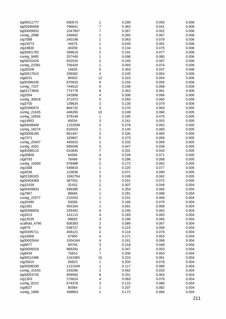
211
tig00011777 930573 1 0.290 0.055 0.006
tig00395658 796641 7 0.363 0.041 0.006
tig00009932 1047807 7 0.367 0.052 0.006
contig_2088 246692 1 0.260 0.067 0.006
ctg7088 240198 1 0.063 0.079 0.006
ctg15573 44675 1 0.045 0.091 0.006
ctg18830 40259 1 0.134 0.075 0.006
tig00001782 399619 2 0.191 0.077 0.006
contig_9485 207449 1 0.098 0.080 0.006
tig00010426 932016 2 0.240 0.067 0.006
contig_22381 756420 1 0.093 0.074 0.006
ctg35208 19926 5 0.353 0.047 0.006
tig00017610 299362 4 0.245 0.054 0.006
ctg8231 80920 12 0.315 0.054 0.006
tig00396435 870933 9 0.150 0.055 0.006
contig_7237 744510 6 0.248 0.068 0.006
tig02173845 774778 8 0.263 0.061 0.006
ctg2054 242868 4 0.308 0.066 0.006
contig_30818 371972 5 0.350 0.060 0.006
ctg3700 139634 2 0.130 0.079 0.006
tig00396970 864732 3 0.270 0.063 0.005
contig_21635 446265 10 0.248 0.068 0.005
contig_10934 379149 1 0.195 0.075 0.005
ctg14952 60034 3 0.241 0.053 0.005
tig00048408 1152938 2 0.278 0.062 0.005
contig_18274 615023 1 0.140 0.083 0.005
tig00008185 861467 3 0.335 0.050 0.005
ctg7371 183667 5 0.273 0.059 0.005
contig_25407 445815 1 0.232 0.069 0.005
contig_4262 585508 5 0.447 0.036 0.005
tig00398115 610845 7 0.331 0.043 0.005
ctg30809 64584 4 0.228 0.071 0.005
ctg8783 78486 5 0.298 0.058 0.005
contig_10059 978488 2 0.172 0.062 0.005
ctg1588 549819 1 0.220 0.077 0.005
ctg4536 123636 1 0.071 0.090 0.005
tig02186325 1062754 3 0.249 0.062 0.005
tig00404369 387001 1 0.201 0.072 0.005
ctg22439 32432 2 0.307 0.049 0.004
tig00409833 599385 1 0.254 0.065 0.004
ctg7967 88666 1 0.281 0.068 0.004
contig_22577 210263 1 0.231 0.069 0.004
ctg20480 50058 1 0.166 0.079 0.004
ctg1581 455164 1 0.091 0.089 0.004
tig00396826 235492 6 0.240 0.062 0.004
ctg3313 141113 4 0.183 0.063 0.004
ctg13535 89820 3 0.196 0.065 0.004
scaffold_4796 508383 2 0.089 0.067 0.004
ctg979 538727 6 0.215 0.069 0.004
tig00395711 406121 2 0.116 0.076 0.004
ctg16906 67950 4 0.271 0.053 0.004
tig00002644 1004164 4 0.241 0.068 0.004
ctg9077 99794 3 0.218 0.048 0.004
tig00006018 889293 2 0.347 0.053 0.004
ctg9434 75810 7 0.206 0.054 0.004
tig00012486 1161965 15 0.210 0.061 0.004
ctg25810 56923 1 0.200 0.078 0.004
tig00398299 1121549 1 0.117 0.089 0.004
contig_31543 243296 2 0.462 0.033 0.004
tig00053745 959500 8 0.201 0.063 0.004
ctg1303 276624 4 0.083 0.076 0.004
contig_8210 674378 3 0.115 0.080 0.004
ctg9027 80364 1 0.207 0.082 0.004
contig_1888 348863 1 0.172 0.084 0.004
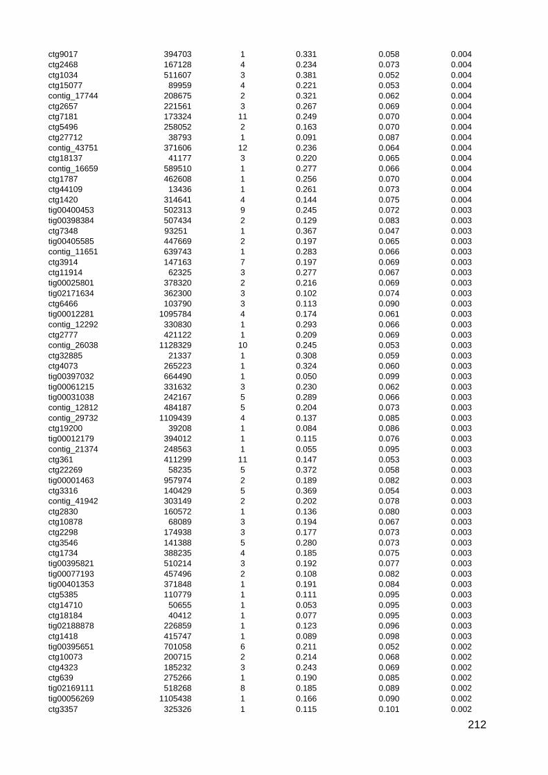
212
ctg9017 394703 1 0.331 0.058 0.004
ctg2468 167128 4 0.234 0.073 0.004
ctg1034 511607 3 0.381 0.052 0.004
ctg15077 89959 4 0.221 0.053 0.004
contig_17744 208675 2 0.321 0.062 0.004
ctg2657 221561 3 0.267 0.069 0.004
ctg7181 173324 11 0.249 0.070 0.004
ctg5496 258052 2 0.163 0.070 0.004
ctg27712 38793 1 0.091 0.087 0.004
contig_43751 371606 12 0.236 0.064 0.004
ctg18137 41177 3 0.220 0.065 0.004
contig_16659 589510 1 0.277 0.066 0.004
ctg1787 462608 1 0.256 0.070 0.004
ctg44109 13436 1 0.261 0.073 0.004
ctg1420 314641 4 0.144 0.075 0.004
tig00400453 502313 9 0.245 0.072 0.003
tig00398384 507434 2 0.129 0.083 0.003
ctg7348 93251 1 0.367 0.047 0.003
tig00405585 447669 2 0.197 0.065 0.003
contig_11651 639743 1 0.283 0.066 0.003
ctg3914 147163 7 0.197 0.069 0.003
ctg11914 62325 3 0.277 0.067 0.003
tig00025801 378320 2 0.216 0.069 0.003
tig02171634 362300 3 0.102 0.074 0.003
ctg6466 103790 3 0.113 0.090 0.003
tig00012281 1095784 4 0.174 0.061 0.003
contig_12292 330830 1 0.293 0.066 0.003
ctg2777 421122 1 0.209 0.069 0.003
contig_26038 1128329 10 0.245 0.053 0.003
ctg32885 21337 1 0.308 0.059 0.003
ctg4073 265223 1 0.324 0.060 0.003
tig00397032 664490 1 0.050 0.099 0.003
tig00061215 331632 3 0.230 0.062 0.003
tig00031038 242167 5 0.289 0.066 0.003
contig_12812 484187 5 0.204 0.073 0.003
contig_29732 1109439 4 0.137 0.085 0.003
ctg19200 39208 1 0.084 0.086 0.003
tig00012179 394012 1 0.115 0.076 0.003
contig_21374 248563 1 0.055 0.095 0.003
ctg361 411299 11 0.147 0.053 0.003
ctg22269 58235 5 0.372 0.058 0.003
tig00001463 957974 2 0.189 0.082 0.003
ctg3316 140429 5 0.369 0.054 0.003
contig_41942 303149 2 0.202 0.078 0.003
ctg2830 160572 1 0.136 0.080 0.003
ctg10878 68089 3 0.194 0.067 0.003
ctg2298 174938 3 0.177 0.073 0.003
ctg3546 141388 5 0.280 0.073 0.003
ctg1734 388235 4 0.185 0.075 0.003
tig00395821 510214 3 0.192 0.077 0.003
tig00077193 457496 2 0.108 0.082 0.003
tig00401353 371848 1 0.191 0.084 0.003
ctg5385 110779 1 0.111 0.095 0.003
ctg14710 50655 1 0.053 0.095 0.003
ctg18184 40412 1 0.077 0.095 0.003
tig02188878 226859 1 0.123 0.096 0.003
ctg1418 415747 1 0.089 0.098 0.003
tig00395651 701058 6 0.211 0.052 0.002
ctg10073 200715 2 0.214 0.068 0.002
ctg4323 185232 3 0.243 0.069 0.002
ctg639 275266 1 0.190 0.085 0.002
tig02169111 518268 8 0.185 0.089 0.002
tig00056269 1105438 1 0.166 0.090 0.002
ctg3357 325326 1 0.115 0.101 0.002

213
tig00010830 362633 6 0.301 0.061 0.002
ctg18249 67394 3 0.311 0.064 0.002
tig00398065 1002344 2 0.117 0.064 0.002
ctg6787 207566 3 0.270 0.070 0.002
ctg4301 131532 2 0.109 0.088 0.002
tig00395688 396431 1 0.238 0.056 0.002
tig00403730 621907 6 0.176 0.073 0.002
ctg1471 202892 4 0.122 0.076 0.002
tig00405347 543473 5 0.157 0.079 0.002
tig02169458 962236 1 0.081 0.090 0.002
ctg2320 432401 4 0.340 0.062 0.002
tig00399539 282857 1 0.224 0.075 0.002
ctg33263 21223 1 0.142 0.082 0.002
ctg468 455220 7 0.161 0.071 0.002
tig02170431 955332 9 0.322 0.072 0.002
ctg13522 167494 2 0.148 0.092 0.002
tig00399738 453577 4 0.336 0.058 0.002
tig02169868 857412 6 0.390 0.061 0.002
ctg5666 344659 7 0.320 0.068 0.002
ctg7065 139213 7 0.251 0.072 0.002
ctg28120 96309 4 0.231 0.073 0.002
tig00399040 611393 2 0.174 0.075 0.002
ctg3157 183320 1 0.139 0.097 0.002
contig_28327 505316 1 0.088 0.100 0.002
tig00403292 917868 7 0.254 0.067 0.002
ctg5478 203258 2 0.305 0.069 0.002
ctg36424 18494 10 0.246 0.077 0.002
ctg3596 175065 5 0.203 0.084 0.002
contig_15985 614099 1 0.170 0.090 0.002
tig00003475 384296 8 0.091 0.094 0.002
tig00397067 1508104 1 0.113 0.095 0.002
tig00404052 254563 3 0.130 0.098 0.002
ctg278 700468 2 0.230 0.078 0.002
tig00015630 444711 3 0.181 0.082 0.002
tig00048729 291077 10 0.186 0.082 0.002
ctg1573 271466 1 0.082 0.100 0.002
contig_1219 625571 4 0.148 0.074 0.002
ctg1727 346568 1 0.128 0.097 0.002
ctg7275 217686 1 0.264 0.072 0.001
tig00395555 271328 8 0.147 0.079 0.001
ctg6355 105304 2 0.101 0.080 0.001
tig00032636 913796 1 0.178 0.082 0.001
tig00074206 384873 5 0.093 0.089 0.001
ctg4652 269717 1 0.150 0.093 0.001
contig_10547 335563 6 0.497 0.037 0.001
contig_8886 292449 3 0.384 0.055 0.001
tig00079487 951179 1 0.361 0.056 0.001
tig02188831 643395 7 0.193 0.060 0.001
tig00014655 351299 10 0.194 0.064 0.001
ctg18756 98018 8 0.309 0.065 0.001
ctg12448 165728 1 0.228 0.085 0.001
ctg20121 36987 1 0.179 0.086 0.001
ctg63201 9826 5 0.354 0.061 0.001
contig_19680 1173980 10 0.338 0.063 0.001
ctg3853 201225 1 0.318 0.070 0.001
tig00058991 244112 4 0.268 0.080 0.001
ctg6611 100866 6 0.160 0.082 0.001
tig00396149 623230 3 0.161 0.088 0.001
tig00397523 322509 3 0.219 0.092 0.001
tig00059977 206712 1 0.143 0.094 0.001
tig00065943 621099 3 0.145 0.101 0.001
ctg36792 18493 5 0.426 0.054 0.001
contig_27491 426366 5 0.267 0.071 0.001
ctg24 616767 8 0.262 0.077 0.001

214
ctg17515 42483 6 0.225 0.079 0.001
contig_2009 241801 1 0.204 0.090 0.001
ctg15643 47287 1 0.140 0.097 0.001
tig00018215 545841 5 0.388 0.057 0.001
ctg4689 205094 2 0.332 0.061 0.001
contig_32639 577279 7 0.228 0.067 0.001
tig02186583 453875 3 0.304 0.075 0.001
ctg1552 326042 1 0.251 0.080 0.001
contig_23904 445721 2 0.154 0.083 0.001
ctg16582 73716 4 0.195 0.086 0.001
ctg9736 109962 2 0.222 0.089 0.001
tig00399227 736035 6 0.195 0.094 0.001
ctg29432 23874 1 0.184 0.097 0.001
tig00399197 524909 1 0.176 0.099 0.001
ctg27879 25595 1 0.161 0.100 0.001
tig00093735 410540 2 0.075 0.108 0.001
ctg4406 125850 1 0.096 0.114 0.001
tig00028029 426442 8 0.385 0.055 0.001
tig00398278 361467 2 0.314 0.079 0.001
ctg4505 299987 3 0.238 0.088 0.001
tig00400420 264576 3 0.176 0.092 0.001
ctg8602 230135 2 0.097 0.122 0.001
ctg9542 77502 7 0.226 0.074 0.001
ctg5718 110930 7 0.264 0.080 0.001
tig00013101 268866 4 0.286 0.082 0.001
tig00027857 700320 2 0.186 0.097 0.001
ctg2079 413176 1 0.087 0.109 0.001
ctg2846 347791 2 0.092 0.113 0.001
tig00399901 811080 2 0.095 0.115 0.001
ctg2517 254880 1 0.098 0.118 0.001
contig_42809 351746 3 0.384 0.067 0.001
ctg1123 237209 3 0.269 0.074 0.001
ctg17685 45882 2 0.137 0.090 0.001
ctg9691 75105 6 0.216 0.090 0.001
ctg6339 334965 1 0.087 0.096 0.001
tig00059998 1068736 4 0.147 0.097 0.001
tig00017035 1132614 1 0.111 0.105 0.001
contig_13674 627862 1 0.077 0.106 0.001
tig02188748 571085 1 0.123 0.109 0.001
ctg3668 526163 2 0.132 0.117 0.001
tig00016009 623372 8 0.192 0.074 0.001
ctg10034 158959 8 0.381 0.075 0.001
tig00404038 641509 4 0.338 0.076 0.001
tig00137030 555776 1 0.305 0.080 0.001
ctg8899 80402 5 0.159 0.081 0.001
ctg9926 78349 4 0.283 0.084 0.001
tig00040441 397931 3 0.304 0.086 0.001
ctg36120 19521 1 0.179 0.093 0.001
tig00044954 583249 1 0.246 0.094 0.001
contig_5520 227618 1 0.245 0.097 0.001
tig00010587 1336264 6 0.193 0.098 0.001
tig00003873 791057 2 0.140 0.110 0.001
ctg27780 25018 1 0.174 0.110 0.001
ctg3120 269904 2 0.107 0.115 0.001
ctg7363 94642 1 0.106 0.116 0.001
contig_27828 686464 2 0.088 0.127 0.001
tig00013376 1099857 7 0.287 0.078 0.000
ctg5649 428367 8 0.167 0.080 0.000
ctg28671 22282 1 0.233 0.083 0.000
contig_37023 1291391 11 0.170 0.084 0.000
tig00001226 634311 20 0.235 0.084 0.000
ctg6281 218505 2 0.306 0.086 0.000
tig00398477 259891 2 0.138 0.086 0.000
tig02186361 536843 3 0.188 0.087 0.000

215
ctg29436 23631 1 0.226 0.091 0.000
ctg5058 134239 4 0.198 0.098 0.000
tig00049631 236709 3 0.185 0.112 0.000
ctg9955 81837 1 0.103 0.123 0.000
tig00034653 482718 1 0.072 0.123 0.000
tig00404607 513569 8 0.441 0.064 0.000
ctg25413 28004 3 0.424 0.068 0.000
ctg2742 317531 6 0.262 0.071 0.000
tig02169698 726794 13 0.232 0.073 0.000
tig02169510 472014 3 0.375 0.074 0.000
ctg7787 251517 3 0.296 0.078 0.000
tig00396258 746857 2 0.298 0.080 0.000
ctg14324 128536 1 0.203 0.085 0.000
ctg242 919531 2 0.182 0.086 0.000
contig_7359 400273 1 0.289 0.090 0.000
ctg2283 220690 11 0.261 0.090 0.000
tig00097609 300704 4 0.217 0.091 0.000
tig00088316 353022 4 0.199 0.091 0.000
ctg2930 323457 3 0.209 0.091 0.000
contig_26461 490084 2 0.292 0.091 0.000
ctg2491 168255 1 0.229 0.093 0.000
ctg442 403501 5 0.327 0.093 0.000
tig00001597 1594731 13 0.162 0.094 0.000
contig_28553 1558221 6 0.149 0.098 0.000
ctg7313 148101 5 0.151 0.100 0.000
ctg17866 41464 3 0.189 0.104 0.000
ctg7640 89382 3 0.083 0.111 0.000
ctg21292 34862 3 0.176 0.116 0.000
tig00010280 1014348 1 0.053 0.127 0.000
tig00396144 1246559 1 0.138 0.134 0.000
tig02186630 446353 5 0.281 0.067 0.000
tig02172233 477601 2 0.261 0.072 0.000
ctg8952 191809 12 0.448 0.073 0.000
ctg4754 226547 11 0.322 0.083 0.000
tig00020219 1582543 11 0.245 0.084 0.000
tig00020340 1636072 18 0.231 0.094 0.000
ctg6541 135355 5 0.258 0.095 0.000
ctg27332 26011 2 0.312 0.096 0.000
tig02169907 763412 2 0.304 0.097 0.000
ctg3368 235164 5 0.221 0.098 0.000
ctg1264 638142 6 0.119 0.101 0.000
ctg4898 121403 5 0.232 0.101 0.000
tig02170127 506055 4 0.346 0.104 0.000
contig_16551 552658 2 0.143 0.107 0.000
tig00013757 853991 1 0.173 0.112 0.000
tig00075283 491848 1 0.145 0.113 0.000
ctg10532 69894 4 0.236 0.118 0.000
ctg9146 121205 1 0.095 0.118 0.000
contig_51218 850550 1 0.142 0.118 0.000
ctg4165 205670 3 0.060 0.120 0.000
scaffold_46548 380348 3 0.172 0.123 0.000
ctg12024 104480 1 0.033 0.123 0.000
ctg15101 50662 1 0.132 0.125 0.000
ctg5822 424876 1 0.109 0.128 0.000
ctg10507 95448 10 0.102 0.129 0.000
tig02171260 684552 1 0.108 0.132 0.000
contig_25543 562659 1 0.050 0.136 0.000
ctg16452 198879 1 0.112 0.140 0.000
ctg357 533628 6 0.163 0.056 0.000
tig00000388 923617 3 0.293 0.077 0.000
contig_48617 1124269 2 0.224 0.081 0.000
ctg5775 214807 2 0.389 0.082 0.000
ctg13657 85231 5 0.369 0.084 0.000
contig_29750 831450 5 0.290 0.087 0.000

216
ctg13760 55398 4 0.370 0.089 0.000
contig_37992 158455 3 0.331 0.089 0.000
tig00398304 649387 7 0.309 0.090 0.000
tig00058741 449223 19 0.202 0.095 0.000
contig_4495 397920 4 0.324 0.095 0.000
tig00396753 694085 3 0.224 0.096 0.000
ctg10465 227629 4 0.139 0.097 0.000
tig00005901 1294013 3 0.209 0.097 0.000
tig00401456 1033341 1 0.271 0.098 0.000
contig_61276 243259 4 0.186 0.101 0.000
contig_8562 432781 2 0.216 0.103 0.000
ctg3025 155776 4 0.225 0.104 0.000
ctg4736 122597 2 0.077 0.105 0.000
ctg2490 469086 2 0.251 0.107 0.000
tig00395886 548602 3 0.264 0.107 0.000
tig02170574 313734 2 0.412 0.108 0.000
tig00396169 493748 14 0.220 0.110 0.000
ctg2000 251686 1 0.269 0.110 0.000
contig_29691 284461 4 0.271 0.111 0.000
tig00026233 282094 4 0.253 0.112 0.000
ctg14856 50818 1 0.291 0.113 0.000
ctg6510 102520 9 0.172 0.115 0.000
tig00396462 579784 3 0.265 0.116 0.000
tig00021261 419760 9 0.115 0.119 0.000
tig02169607 499162 8 0.152 0.119 0.000
tig02169928 928537 1 0.168 0.119 0.000
tig02169869 646305 1 0.166 0.122 0.000
tig00403326 206754 2 0.160 0.122 0.000
ctg6506 116431 8 0.127 0.123 0.000
ctg18711 39811 1 0.130 0.123 0.000
contig_22489 632453 1 0.190 0.128 0.000
ctg2589 368501 1 0.242 0.128 0.000
ctg4460 127493 3 0.181 0.129 0.000
ctg11469 84175 1 0.056 0.129 0.000
ctg1560 212380 1 0.120 0.131 0.000
ctg27349 22608 1 0.126 0.132 0.000
ctg8445 100647 1 0.037 0.133 0.000
contig_6378 651179 1 0.126 0.133 0.000
tig00400477 444752 4 0.131 0.133 0.000
contig_8232 217362 2 0.129 0.134 0.000
ctg852 248256 1 0.233 0.134 0.000
tig00058036 278178 3 0.038 0.135 0.000
contig_2548 273877 1 0.109 0.135 0.000
tig00402075 327274 3 0.203 0.136 0.000
ctg3372 143161 9 0.105 0.137 0.000
ctg12268 112660 3 0.269 0.137 0.000
ctg3169 476323 1 0.051 0.137 0.000
ctg4011 492880 1 0.052 0.137 0.000
ctg1519 240218 1 0.114 0.138 0.000
contig_4079 720163 7 0.229 0.138 0.000
tig00047947 229809 3 0.184 0.140 0.000
ctg8829 91237 2 0.191 0.142 0.000
tig00014963 470209 1 0.051 0.143 0.000
tig00047492 311084 1 0.086 0.144 0.000
tig00058221 370517 4 0.106 0.146 0.000
ctg2243 494601 1 0.304 0.146 0.000
ctg3407 229476 1 0.238 0.148 0.000
ctg287 682863 3 0.161 0.148 0.000
tig00395743 912175 3 0.339 0.149 0.000
ctg7939 119940 6 0.237 0.149 0.000
ctg6440 331778 1 0.211 0.149 0.000
ctg21626 68466 10 0.204 0.150 0.000
contig_37029 817425 6 0.192 0.150 0.000
ctg6609 154333 1 0.214 0.151 0.000

217
tig00395657 765970 1 0.129 0.154 0.000
ctg9541 75157 2 0.140 0.157 0.000
tig02175166 365575 1 0.129 0.157 0.000
tig00402739 313999 1 0.195 0.163 0.000
ctg3235 286464 1 0.121 0.166 0.000
ctg34396 20111 1 0.229 0.168 0.000
contig_17548 267555 1 0.104 0.168 0.000
ctg172 532540 13 0.169 0.168 0.000
ctg14352 72360 1 0.068 0.169 0.000
ctg9474 221587 2 0.033 0.174 0.000
contig_16540 228155 4 0.184 0.174 0.000
contig_3123 1138239 5 0.247 0.177 0.000
ctg12338 77367 1 0.189 0.179 0.000
ctg3990 216494 1 0.123 0.182 0.000
ctg11806 64035 1 0.195 0.184 0.000
ctg4256 486192 1 0.102 0.185 0.000
tig00006227 805723 3 0.259 0.192 0.000
ctg10925 67646 1 0.116 0.193 0.000
tig00028442 531138 1 0.040 0.200 0.000
ctg7090 171446 2 0.089 0.208 0.000
ctg17967 73963 1 0.119 0.242 0.000
tig00395900 652960 2 0.105 0.253 0.000

218
Chapter 4:
Figure S4.1: Present-day distribution of pale-lipped shell morphs in four Pyrenean
valleys. Pie charts show frequencies of pale-lipped shells (white) versus other forms.
Figure S4.2: Scatterplots showing the present-day relationship between altitude and
frequency of pale-lipped morphs in four Pyrenean valleys. Regression line and
confidence intervals are shown, alongside the Pearson coefficient and p value.
Figure S4.3: Scatterplots showing the present-day relationship between altitude and
size and shape of shells in four Pyrenean valleys. Regression line and confidence
intervals are shown, alongside the Pearson coefficient and p value.
Figure S4.4: Scatterplot showing variation of visual space coordinates, xyz, on three
principal component axes, using shells from Vielha and Jueu valleys in the
Pyrenees. Units are in JNDs. Points are coloured according to human-scored
classification of the shell, either yellow or pink.
Table S4.1: Summary of the Pyrenean sampling collection of 2017 and 2018.
Geographical and habitat details are shown, further with the summary of shell
phenotypes.
Table S4.2: Summary of the historical collections in the Pyrenees provided by the
Evolution Megalab team. Geographical and habitat details are shown, further with
the summary of shell phenotypes.
Table S4.3: Direction of change in shell morph frequencies, from 1960s to
2017/2018 in the Pyrenees.
Table S4.4: Statistical summary of shell altitudinal distribution in each valley;
correlations (Pearson, parametric; Kendall, non-parametric).
Supplementary material: The qualitative phenotype and quantitative reflectance
data for the samples used in this study can be access by request.

219
Figure S4.1. Present-day distribution of pale-lipped shell morphs in four Pyrenean valleys. Pie charts
show frequencies of pale-lipped shells (white) versus other forms.

220
Figure S4.2. Scatterplots showing the present-day relationship between altitude and frequency of
pale-lipped morphs in four Pyrenean valleys. Regression line and confidence intervals are shown,
alongside the Pearson coefficient and p value.

221
Figure S4.3. Scatterplots showing the present-day relationship between altitude and size and shape of shells in four Pyrenean valleys. Regression line and
confidence intervals are shown, alongside the Pearson coefficient and p value.

222
Figure S4.4. Scatterplot showing variation of visual space coordinates, xyz, on three principal
component axes, using shells from Vielha and Jueu valleys in the Pyrenees. Units are in JNDs. Points
are coloured according to human-scored classification of the shell, either yellow or pink.

223
Table S4.1. Summary of the sampling collection of C. nemoralis in 2017 and 2018. Details of location, habitat and shell phenotypes with its frequencies are reported.
Code Latitude Longitude Altitude Habitat Total Yellow Pink Brown Unbanded Mid-banded Five-banded Other banding
classification snails
2017 collection
DRG1 42.69676 0.81278 1014 2 34 22 12 0 5 2 23 4
DRG2 42.69723 0.81273 1027 1 9 9 0 0 2 0 5 2
DRG3 42.69939 0.82452 1016 1 14 7 6 0 5 0 9 0
DRG4 42.70123 0.92666 1458 1 30 18 12 0 3 0 27 0
DRG5 42.70094 0.92759 1459 2 46 26 20 0 2 4 36 4
DRG6 42.69719 0.93143 1433 2 12 10 2 0 4 0 8 0
DRG7 42.69985 0.91832 1318 2 22 13 10 0 9 2 11 0
DRG8 42.69996 0.91832 1321 1 8 6 2 0 3 0 4 1
DRG9 42.70002 0.91755 1344 2 9 5 4 0 1 1 7 0
DRG10 42.70415 0.90238 1275 2 23 15 8 0 2 1 15 5
DRG11 42.70504 0.90342 1234 1 17 2 15 0 2 0 15 0
DRG12 42.69854 0.86332 1129 1 21 11 10 0 10 2 8 1
DRG13 42.70004 0.84889 1113 2 62 41 21 0 5 0 55 2
DRG14 42.67835 0.87315 1261 1 37 37 0 0 20 0 14 3
DRG15 42.68278 0.87539 1259 2 23 22 1 0 21 0 2 0
DRG16 42.69085 0.87381 1202 2 18 13 5 0 3 2 12 1
DRG17 42.69048 0.87416 1178 3 63 42 21 0 32 3 27 1
DRG18 42.69539 0.87371 1138 1 43 31 10 0 5 2 30 6
DRG19 42.68952 0.78683 1193 2 1 1 0 0 1 0 0 0
DRG20 42.67758 0.78686 1229 1 16 16 0 0 14 0 0 2
DRG21 42.67866 0.78779 1212 1 15 15 0 0 10 0 5 0
DRG22 42.68685 0.78983 1166 1 10 8 2 0 4 0 2 4
DRG23 42.68785 0.79002 1148 1 14 16 0 0 6 2 4 2
DRG24 42.6988 0.79402 1006 1 39 35 4 0 10 1 26 2
DRG25 42.69666 0.79275 978 2 14 15 2 0 2 1 9 2
DRG26 42.70031 0.80295 958 1 13 8 5 0 4 0 5 4
DRG27 42.70686 0.79624 961 2 56 35 19 0 3 2 49 2
DRG28 42.72042 0.79612 1007 3 30 21 8 0 5 6 18 1
DRG29 42.72947 0.79178 1147 2 10 9 1 0 1 0 9 0
DRG30 42.72604 0.79948 1222 2 10 7 3 0 8 1 1 0

224
DRG31 42.72174 0.79331 975 2 4 3 1 0 1 2 1 0
DRG32 42.7265 0.78439 925 2 43 13 30 0 9 2 31 1
DRG33 42.72649 0.78841 932 1 22 18 4 0 10 0 12 0
DRG34 42.73341 0.77671 909 1 22 15 7 0 1 1 20 0
DRG35 42.73886 0.76158 884 2 10 5 5 0 1 4 5 0
DRG36 42.73657 0.76037 877 2 24 16 8 0 13 1 6 4
DRG37 42.70649 0.80882 1423 1 10 7 3 0 0 0 8 2
DRG38 42.74539 0.70552 823 2 17 7 10 0 4 3 6 4
DRG39 42.73815 0.72204 838 3 16 8 8 0 7 0 9 0
DRG40 42.73626 0.72043 872 3 11 4 7 0 0 0 10 1
DRG41 42.7158 0.72163 1035 3 3 2 1 0 2 1 0 0
DRG42 42.70236 0.71194 1156 1 204 184 20 0 39 27 54 84
DRG43 42.6972 0.70773 1226 1 6 5 1 0 1 0 1 4
DRG44 42.67711 0.70696 1396 3 9 9 0 0 9 0 0 0
DRG45 42.68214 0.70667 1432 1 23 21 2 0 23 0 0 0
DRG46 42.68289 0.70754 1280 3 18 16 2 0 12 0 6 0
DRG47 42.71797 0.72336 1033 1 30 26 3 0 10 5 14 1
DRG48 42.7061 0.913922 1387 1 15 7 8 0 0 0 15 0
DRG49 42.70468 0.924582 1612 1 20 8 12 0 2 0 18 0
DRG50 42.5639 0.75003 1349 2 33 32 1 0 33 0 0 0
DRG51 42.55828 0.74746 1297 2 2 0 2 0 2 0 0 0
DRG52 42.55217 0.74768 1243 2 10 9 1 0 9 0 1 0
DRG53 42.54617 0.73439 1206 2 1 0 1 0 1 0 0 0
DRG54 42.54703 0.74149 1194 2 16 16 0 0 16 0 0 0
DRG55 42.54463 0.73038 1164 1 1 1 0 0 1 0 0 0
DRG56 42.54065 0.72912 1094 2 17 9 7 1 16 0 1 0
DRG57 42.53904 0.72736 1055 2 9 8 0 1 9 0 0 0
DRG58 42.53669 0.72622 1071 2 23 23 0 0 23 0 0 0
DRG59 42.53588 0.72553 1065 2 17 14 3 0 15 0 2 0
DRG60 42.51323 0.71942 1036 1 11 11 0 0 9 0 2 0
DRG61 42.513 0.71964 1036 2 19 10 0 9 18 0 1 0
DRG62 42.5064 0.71806 991 2 29 23 1 5 27 0 2 0
DRG63 42.41283 0.74002 883 1 43 28 8 7 13 3 22 5
DRG64 42.41867 0.73595 870 3 21 31 0 0 20 0 0 1
DRG65 42.41888 0.73597 865 2 5 5 0 0 3 0 0 2
DRG66 42.42711 0.72841 871 2 4 1 0 3 4 0 0 0
DRG67 42.43095 0.72259 869 2 11 11 0 0 11 0 0 0

225
DRG68 42.43537 0.71466 905 2 10 10 0 0 8 0 2 0
DRG69 42.43527 0.71464 892 2 10 5 0 5 9 0 1 0
DRG70 42.44844 0.71035 957 1 12 9 0 3 12 0 0 0
DRG71 42.45884 0.70997 937 2 14 12 2 0 8 0 6 0
DRG72 42.46839 0.71497 1029 2 3 0 0 3 3 0 0 0
DRG74 42.48304 0.71561 974 2 13 5 1 7 10 0 3 0
DRG75 42.48171 0.7147 978 2 16 3 0 13 16 0 0 0
DRG77 42.4792 0.71395 946 2 31 17 2 12 23 0 8 0
DRG78 42.43259 0.73986 905 2 44 35 4 5 23 1 13 7
DRG79 42.43479 0.74287 862 2 17 16 1 0 12 3 2 0
DRG80 42.44119 0.74672 909 1 10 10 0 0 8 1 1 0
DRG81 42.44796 0.7519 869 1 12 12 0 0 6 1 4 1
DRG82 42.45299 0.75418 941 2 17 15 2 0 8 0 7 2
DRG83 42.45321 0.75442 938 2 12 7 1 0 2 0 4 6
DRG84 42.45633 0.75849 996 1 32 35 0 0 6 3 15 8
DRG85 42.45556 0.75928 953 3 40 37 3 0 3 2 32 3
DRG86 42.45626 0.76009 961 1 47 45 2 0 8 1 29 9
DRG87 42.46047 0.76597 931 1 6 6 0 0 3 2 1 0
DRG88 42.49438 0.784053 1115 2 24 22 2 0 7 1 12 4
DRG89 42.49937 0.78319 1189 2 5 5 0 0 0 0 5 0
DRG90 42.49679 0.78401 1173 2 44 43 1 0 7 5 32 0
DRG91 42.49706 0.78695 1118 2 10 10 0 0 6 1 3 0
DRG92 42.56332 0.84286 1070 1 19 16 0 3 10 3 5 1
DRG93 42.5569 0.83714 1428 3 14 14 0 0 8 3 1 2
DRG94 42.54425 0.83964 1374 1 3 2 1 0 1 0 0 2
DRG95 42.52676 0.83342 1298 1 12 12 0 0 0 2 10 0
DRG96 42.52313 0.83568 1304 2 14 14 0 0 0 3 11 0
DRG97 42.52317 0.83659 1309 1 11 11 0 0 0 1 10 0
DRG98 42.52018 0.84257 1380 1 19 19 0 0 0 0 19 0
DRG99 42.51924 0.84682 1463 2 6 6 0 0 0 0 6 0
DRG100 42.52649 0.82871 1219 1 22 21 1 0 1 3 16 2
DRG101 42.51701 0.81945 1105 1 41 35 6 0 11 8 18 4
DRG102 42.50738 0.80655 1097 2 42 41 1 0 4 2 34 2
2018 collection
DRG103 42.67786 0.705514 1474 2 19 12 7 0 15 0 4 0

226
DRG104 42.67605 0.705895 1480 2 6 6 0 0 6 0 0 0
DRG105 42.67509 0.702944 1494 1 6 6 0 0 2 0 4 0
DRG106 42.67439 0.702068 1559 2 27 27 0 0 27 0 0 0
DRG107 42.6747 0.7013 1527 2 19 19 0 0 19 0 0 0
DRG108 42.674 0.6999 1555 2 12 11 1 0 12 0 0 0
DRG109 42.6697 0.6999 1688 2 16 16 0 0 16 0 0 0
DRG110 42.6665 0.6947 1921 2 3 3 0 0 3 0 0 0
DRG111 42.6697 0.7089 1554 2 6 6 0 0 6 0 0 0
DRG112 42.674 10.7122 1565 2 14 14 0 0 14 0 0 0
DRG113 42.6751 0.7075 1512 3 6 6 0 0 6 0 0 0
DRG114 42.67762 0.707189 1482 3 10 8 2 0 3 0 6 1
DRG115 42.68255 0.70815 1450 2 13 13 0 0 3 0 3 7
DRG116 42.6907 0.708 1392 2 7 7 0 0 6 0 1 0
DRG117 42.7024 0.7123 1299 2 10 8 2 0 2 0 4 4
DRG118 42.70423 0.93945 1714 2 5 5 0 0 1 0 4 0
DRG119 42.70345 0.94682 1760 2 3 3 0 0 3 0 0 0
DRG120 42.70115 0.944631 1751 2 3 3 0 0 3 0 0 0
DRG121 42.699 0.9461 1844 2 1 1 0 0 1 0 0 0
DRG122 42.703 0.9433 1859 2 2 2 0 0 2 0 0 0
DRG123 42.72038 0.916398 1582 1 28 13 15 0 1 0 27 0
DRG124 42.6214 0.765843 1586 2 22 12 10 0 15 0 4 3
DRG125 42.62202 0.764279 1520 2 5 0 4 1 2 1 1 1
DRG126 42.7211 0.9142 1396 1 29 21 8 0 0 0 27 2
DRG127 42.71366 0.914242 1365 2 24 11 13 0 0 0 24 0
DRG128 42.7122 0.9104 1355 2 15 15 0 0 5 0 9 1
DRG129 42.7113 0.905847 1325 1 11 8 3 0 0 0 11 0
DRG130 42.7007 0.8628 1254 1 49 34 15 0 4 3 41 1
DRG131 42.5693 0.8465 1635 2 3 3 0 0 0 0 3 0
DRG132 42.5693 0.8465 1635 2 2 2 0 0 0 0 1 1
DRG133 42.56637 0.845173 1502 2 19 19 0 0 16 1 2 0
DRG134 42.56669 0.845923 1524 2 10 10 0 0 6 0 4 0
DRG135 42.56332 0.84286 1478 2 24 23 1 0 8 5 10 1
DRG136 42.55371 0.83521 1410 2 18 16 2 0 14 1 2 1
DRG137 42.54425 0.83964 1334 2 21 20 1 0 7 0 14 2
DRG138 42.5311 0.8346 1281 2 18 17 1 0 3 0 15 4

227
Sites from 2017 resampled in 2018
DRG10 42.70415 0.90238 1275 2 30 19 11 0 3 0 27 0
DRG42 42.70236 0.71194 1156 2 73 70 3 0 14 13 46 24
DRG75 42.48171 0.7147 978 2 26 8 0 18 25 0 1 0
DRG77 42.4792 0.71395 946 2 46 23 0 23 40 0 6 0
DRG100 42.52649 0.82871 1219 1 17 17 0 0 0 0 17 0
Total summary of resampled sites
DRG10 42.70415 0.90238 1275 2 53 34 19 0 5 1 42 5
DRG42 42.70236 0.71194 1156 2 277 254 23 0 53 40 100 84
DRG75 42.48171 0.7147 978 2 42 11 0 31 41 0 1 0
DRG77 42.4792 0.71395 946 2 77 40 2 35 63 0 14 0
DRG100 42.52649 0.82871 1219 1 39 38 1 0 1 3 33 2
Habitat classification; 1 = Open (shrubland, walls, grassland), 2 =Hedgerow or tall herbs, 3 = Woodland or shaded areas.

228
Table S4.2. Summary of the historical data for C. nemoralis . Details of location, habitat and shell phenotypes with its frequencies are reported.
Code Year Latitude Longitude Altitude Total snails Yellow Pink Brown Unbanded Mid-banded Five-banded
Arnold, RW 1968 Phil.Trans.R.Soc.Lond B 253, 549-593
AR1 1962 42.8631 0.7464 683 40 15 25 0 6 3 31
AR2 1962 42.8381 0.7306 722 28 6 22 0 1 7 20
AR3 1962 42.8106 0.7107 837 29 16 13 0 2 6 21
AR4 1962 42.7959 0.6993 772 27 20 7 0 2 0 25
AR5 1962 42.7891 0.6956 873 54 37 17 0 4 7 43
AR6 1962 42.7755 0.6866 788 36 27 9 0 5 3 28
AR7 1962 42.76139 0.6858 931 36 21 15 0 5 5 26
AR8 1962 42.75 0.7031 941 35 15 20 0 3 5 27
AR9 1962 42.7407 0.7146 849 51 29 22 0 14 2 35
AR10 1962 42.7389 0.7278 936 59 39 20 0 12 3 44
AR11 1962 42.7381 0.7455 905 51 29 22 0 8 3 40
AR12 1962 42.7392 0.7579 940 42 24 18 0 5 1 36
AR13 1962 42.7345 0.7724 1100 27 11 16 0 4 1 22
AR14 1962 42.723 0.7807 1016 39 19 20 0 3 2 34
AR15 1962 42.7256 0.7862 1217 41 23 18 0 3 5 33
AR16 1962 42.7142 0.7963 1186 61 39 22 0 21 4 36
AR17 1962 42.7089 0.7949 1186 35 20 15 0 1 3 31
AR18 1962 42.7006 0.7989 1073 32 18 14 0 4 0 28
AR19 1962 42.6976 0.8095 1067 45 18 27 0 2 6 37
AR20 1962 42.6974 0.8229 1126 39 23 16 0 7 0 32
AR21 1962 42.6998 0.835 1217 74 63 11 0 23 5 46
AR22 1962 42.7001 0.8466 1306 58 31 27 0 2 1 55
AR23 1962 42.7007 0.8628 1254 58 27 31 0 4 2 52
AR24 1962 42.7012 0.8683 1232 65 32 33 0 8 3 54
AR25 1962 42.7025 0.8868 1256 70 37 33 0 5 0 65
AR26 1962 42.7059 0.8921 1273 76 43 33 0 9 2 65
AR27 1962 42.7067 0.9012 1321 44 20 24 0 0 0 44
AR28 1962 42.7027 0.9119 1426 43 18 25 0 6 0 37

229
AR29 1962 42.7004 0.9179 1548 83 43 40 0 27 4 52
AR30 1962 42.6994 0.9213 1493 45 32 13 0 26 1 18
AR31 1962 42.6981 0.9259 1522 32 28 4 0 23 0 9
AR32 1962 42.6973 0.929 1522 63 52 11 0 54 2 7
AR33 1962 42.6949 0.9369 1793 66 61 5 0 64 0 2
AR34 1962 42.6916 0.9404 1534 28 23 5 0 26 0 2
AR35 1962 42.732 0.7265 1197 48 43 5 0 19 4 25
AR36 1962 42.722 0.7248 1103 29 25 4 0 7 8 14
AR37 1962 42.7086 0.717 1508 47 42 5 0 19 2 26
AR38 1962 42.6958 0.7091 1465 49 25 24 0 41 6 2
AR39 1962 42.6723 0.7047 1527 44 44 0 0 43 0 1
AR40 1962 42.7419 0.7551 1085 37 35 2 0 6 3 28
AR41 1962 42.7466 0.7593 1418 29 29 0 0 13 0 16
AR42 1962 42.7519 0.7625 1169 26 25 1 0 24 0 2
AR43 1962 42.7587 0.772 1278 9 9 0 0 8 0 1
AR44 1962 42.7655 0.7756 1720 21 13 8 0 20 0 1
AR45 1962 42.7667 0.7799 1367 23 21 2 0 22 0 1
AR46 1962 42.7193 0.8017 1280 51 27 24 0 8 6 37
AR47 1962 42.7208 0.8051 1280 25 18 7 0 2 0 23
AR48 1962 42.7242 0.8089 1554 68 63 5 0 19 0 49
AR49 1962 42.7288 0.8162 1357 29 29 0 0 16 1 12
AR50 1962 42.7305 0.82 1586 30 28 2 0 17 1 12
AR51 1962 42.731 0.8248 1586 37 37 0 0 35 1 1
AR52 1962 42.7328 0.8216 1586 36 36 0 0 33 1 2
AR53 1962 42.7338 0.8204 1731 32 32 0 0 25 0 7
AR54 1962 42.7362 0.8214 1731 49 49 0 0 49 0 0
AR55 1962 42.7399 0.8221 1731 24 24 0 0 24 0 0
AR56 1962 42.7426 0.8226 1951 17 17 0 0 17 0 0
AR57 1962 42.6891 0.7932 1473 48 40 8 0 21 6 21
AR58 1962 42.6947 0.7904 1110 44 37 7 0 19 6 19
AR59 1962 42.6898 0.7897 1358 87 80 7 0 56 9 22
AR60 1962 42.6859 0.7887 1358 20 20 0 0 18 1 1
AR61 1962 42.6794 0.7876 1531 65 64 1 0 48 7 10

230
AR62 1962 42.6779 0.7863 1531 37 37 0 0 33 0 4
AR63 1962 42.6757 0.7787 1268 6 6 0 0 6 0 0
AR64 1962 42.6754 0.7749 1401 42 42 0 0 42 0 0
AR65 1962 42.6783 0.7689 1401 29 29 0 0 29 0 0
AR66 1962 42.6748 0.765 1552 43 43 0 0 43 0 0
AR67 1962 42.6967 0.8735 1338 32 27 5 0 25 0 7
AR68 1962 42.6953 0.872 1338 45 44 1 0 39 1 5
AR69 1962 42.6922 0.873 1338 36 36 0 0 36 0 0
AR70 1962 42.69 0.8757 1798 25 25 0 0 20 0 5
AR71 1962 42.687 0.8733 1396 23 23 0 0 18 0 5
AR72 1962 42.68 0.8724 1432 28 18 10 0 23 0 5
AR73 1962 42.675 0.8733 1566 32 32 0 0 27 0 5
AR74 1962 42.67 0.8699 1566 27 27 0 0 11 3 13
AR75 1962 42.666 0.8673 1584 24 24 0 0 6 6 12
AR76 1962 42.7122 0.9104 1619 52 38 14 0 5 0 47
AR77 1962 42.7211 0.9142 1520 41 36 5 0 28 1 12
AR78 1962 42.7488 0.9143 1836 46 44 2 0 20 2 24
AR79 1962 42.7583 0.9111 2070 31 31 0 0 30 0 1
AR80 1962 42.7626 0.9122 2307 38 38 0 0 32 0 6
AR81 1962 42.6982 0.9167 1493 54 52 2 0 29 3 22
AR82 1962 42.693 0.9146 1447 28 27 1 0 26 0 2
AR83 1962 42.6832 0.9153 1610 28 28 0 0 25 1 2
AR84 1962 42.6793 0.9153 1610 33 31 2 0 31 1 1
AR85 1962 42.7007 0.937 1803 21 21 0 0 17 1 3
AR86 1962 42.703 0.9433 1859 39 39 0 0 38 0 1
AR87 1962 42.7065 0.955 1918 34 34 0 0 34 0 0
AR88 1962 42.7056 0.9659 2006 30 30 0 0 30 0 0
AR89 1962 42.786 0.7098 1265 21 14 7 0 2 7 12
AR90 1962 42.7605 0.705 1447 24 16 8 0 0 2 22
AR91 1962 42.746 0.7306 1247 31 29 2 0 0 0 31
AR92 1962 42.7447 0.7361 1201 37 23 14 0 0 0 37
AR93 1962 42.743 0.7416 1201 20 12 8 0 3 1 16
AR94 1962 42.7371 0.7766 1269 36 33 3 0 2 2 32

231
AR95 1962 42.7268 0.7896 1217 54 35 19 0 2 2 50
AR96 1962 42.7228 0.7943 1085 71 49 22 0 5 0 66
AR97 1962 42.7133 0.7908 971 59 54 5 0 10 0 49
AR98 1962 42.7059 0.7886 972 70 40 30 0 4 2 64
AR99 1962 42.6956 0.7995 1055 41 31 10 0 4 5 32
AR100 1962 42.7087 0.9076 1376 48 29 19 0 1 0 47
AR101 1962 42.7107 0.91 1619 66 53 13 0 4 0 62
AR102 1962 42.7112 0.9125 1619 61 40 21 0 1 1 59
AR103 1962 42.7125 0.9151 1619 40 36 4 0 2 0 38
AR104 1962 42.7133 0.9174 1885 35 27 8 0 1 0 34
AR105 1962 42.7138 0.919 1885 34 29 5 0 9 0 25
AR106 1962 42.714 0.9204 1885 42 32 10 0 18 0 24
AR107 1962 42.7146 0.9221 1885 30 30 0 0 22 1 7
AR108 1962 42.6953 0.9395 1793 57 56 1 0 41 0 16
AR109 1962 42.697 0.9429 1998 34 33 1 0 27 0 7
AR110 1962 42.699 0.9461 1998 33 33 0 0 33 0 0
AR111 1962 42.7003 0.9517 1918 28 28 0 0 28 0 0
AR112 1962 42.7021 0.9589 2006 54 51 3 0 54 0 0
AR113 1962 42.6978 0.7057 1256 33 27 6 0 21 0 12
AR114 1962 42.7557 0.7629 1169 11 10 1 0 8 0 3
AR115 1962 42.7642 0.7694 1278 22 22 0 0 22 0 0
AR116 1962 42.7252 0.8068 1304 67 61 6 0 8 2 57
AR117 1962 42.6976 0.7892 1110 29 23 6 0 7 2 20
AR118 1962 42.6786 0.7854 1531 32 28 4 0 8 2 22
AR119 1962 42.6963 0.8753 1464 33 21 12 0 0 0 33
AR120 1962 42.6954 0.8772 1464 38 35 3 0 16 1 21
AR121 1962 42.6942 0.8777 1464 90 81 9 0 15 4 71
AR122 1962 42.7207 0.9151 1520 59 42 17 0 7 0 52
AR123 1962 42.7408 0.8209 1731 26 26 0 0 25 0 1
Cameron RAD, Carter, MA, Haynes, FN 1973 Heredity 31, 43-74
CA1 1966 42.7304 0.7256 1197 24 20 4 0 4 3 17
CA2 1966 42.7297 0.7284 1197 27 23 4 0 9 5 13

232
CA3 1966 42.7201 0.7275 1271 24 19 5 0 15 3 6
CA4 1966 42.7145 0.7234 1508 36 32 4 0 20 0 16
CA5 1966 42.712 0.7229 1508 75 57 18 0 19 10 46
CA6 1966 42.7106 0.7197 1508 58 24 34 0 11 17 30
CA7 1966 42.7084 0.7175 1508 84 80 4 0 25 8 51
CA8 1966 42.7042 0.7142 1299 26 25 1 0 7 0 19
CA9 1966 42.7027 0.7132 1299 81 73 8 0 16 3 62
CA10 1966 42.6995 0.7133 1465 30 27 3 0 18 2 10
CA11 1966 42.6861 0.7117 1736 36 19 17 0 36 0 0
CA12 1966 42.6751 0.7046 1512 37 37 0 0 37 0 0
CA13 1966 42.6751 0.7027 1512 43 43 0 0 43 0 0
CA14 1966 42.6747 0.7013 1527 25 25 0 0 25 0 0
CA15 1966 42.674 0.6999 1655 22 22 0 0 22 0 0
CA16 1966 42.6751 0.7108 1915 27 27 0 0 27 0 0
CA17 1966 42.674 0.7122 1943 47 47 0 0 46 0 1
CA18 1966 42.3367 0.7703 1165 19 7 12 0 12 2 5
CA19 1966 42.6294 0.7703 1845 14 1 13 0 9 1 4
CA20 1966 42.6277 0.7731 1845 13 4 9 0 12 0 1
CA21 1966 42.6244 0.766 1651 42 18 24 0 33 0 9
CA22 1966 42.6074 0.7691 1824 22 4 18 0 22 0 0
CA23 1966 42.5862 0.7596 1769 47 46 1 0 47 0 0
CA24 1966 42.5752 0.7631 1805 71 69 2 0 71 0 0
CA25 1966 42.5718 0.756 1445 46 40 0 6 46 0 0
CA26 1966 42.5616 0.7476 1301 47 25 2 20 47 0 0
CA27 1966 42.5549 0.7453 1333 60 60 0 0 60 0 0
CA28 1966 42.5481 0.7298 1149 57 39 8 10 57 0 0
CA29 1966 42.5447 0.7226 1258 27 19 8 0 27 0 0
CA30 1966 42.5404 0.7203 1070 49 28 15 6 49 0 0
CA31 1966 42.5184 0.7191 1143 74 71 0 3 53 14 7
CA32 1966 42.5082 0.7138 1068 84 68 5 11 84 0 0
CA33 1966 42.4879 0.7155 1044 30 12 1 17 29 0 1
CA34 1966 42.4726 0.7119 1090 45 21 0 24 43 0 2
CA35 1966 42.482 0.7155 1008 29 28 1 0 21 2 6

233
CA36 1966 42.5803 0.8596 2435 16 16 0 0 9 0 7
CA37 1966 42.5566 0.8365 1815 13 13 0 0 10 2 1
CA38 1966 42.5515 0.8369 1815 34 29 5 0 27 1 6
CA39 1966 42.5274 0.8298 1447 32 29 3 0 8 2 22
CA40 1966 42.521 0.8274 1327 108 108 0 0 53 1 54
CA41 1966 42.5099 0.8007 1109 136 128 8 0 18 14 104
CA42 1966 42.4989 0.7903 1198 77 73 4 0 12 4 61
CA43 1966 42.476 0.775 1330 42 41 1 0 15 3 24
CA44 1966 42.4689 0.7698 1037 50 50 0 0 8 4 38
CA45 1966 42.465 0.7579 1107 21 21 0 0 20 0 1
CA46 1966 42.4591 0.7441 1261 36 29 7 0 22 4 10
CA47 1966 42.4472 0.7369 1006 37 34 3 0 32 1 4
CA48 1966 42.4342 0.7298 1020 97 88 4 5 86 2 9
CA49 1969 42.7418 0.7042 941 27 19 8 0 6 1 20
CA50 1969 42.7432 0.7075 941 102 56 46 0 15 6 81
CA51 1969 42.743 0.7099 1136 57 45 12 0 8 0 49
CA52 1969 42.7382 0.7108 849 39 28 11 0 6 4 29
CA53 1969 42.7365 0.7142 849 34 28 6 0 4 1 29
CA54 1969 42.7184 0.726 1271 29 22 7 0 14 5 10
CA55 1969 42.7159 0.7246 1508 39 36 3 0 3 14 22
CA56 1969 42.7095 0.7184 1508 36 30 6 0 18 2 16
CA57 1969 42.7024 0.7123 1299 49 25 24 0 12 9 28
CA58 1969 42.6995 0.7134 1465 43 34 9 0 24 2 17
CA59 1969 42.6971 0.7124 1465 30 29 1 0 10 1 19
CA60 1969 42.6946 0.708 1256 53 52 1 0 19 7 27
CA61 1969 42.6935 0.7108 1465 18 14 4 0 12 4 2
CA62 1969 42.6903 0.7113 1736 8 2 6 0 8 0 0
CA63 1969 42.6907 0.708 1392 38 35 3 0 16 0 22
CA64 1969 42.685 0.7096 1736 51 33 18 0 51 0 0
CA65 1969 42.6835 0.7104 1736 40 29 11 0 39 1 0
CA66 1969 42.6697 0.6999 1655 20 20 0 0 20 0 0
CA67 1969 42.6655 0.6966 2180 28 28 0 0 28 0 0
CA68 1969 42.6665 0.6947 2180 17 17 0 0 17 0 0

234
CA69 1969 42.6697 0.7089 1943 20 20 0 0 20 0 0
CA70 1969 42.6672 0.7056 1527 27 27 0 0 27 0 0
CA71 1969 42.663 0.7122 2155 25 25 0 0 25 0 0
CA72 1969 42.6623 0.7108 2155 27 27 0 0 27 0 0
CA73 1969 42.6609 0.7099 2155 23 23 0 0 23 0 0
CA74 1969 42.6751 0.7075 1512 30 30 0 0 30 0 0
CA75 1969 42.6294 0.7667 1845 36 20 16 0 36 0 0
CA76 1969 42.5955 0.7638 1783 16 7 9 0 16 0 0
CA77 1969 42.5815 0.7631 1805 65 60 5 0 65 0 0
CA78 1969 42.5781 0.7627 1805 40 40 0 0 40 0 0
CA79 1969 42.5693 0.7536 1445 22 22 0 0 22 0 0
CA80 1969 42.5642 0.7488 1301 37 26 9 2 37 0 0
CA81 1969 42.5515 0.7388 1296 26 26 0 0 26 0 0
CA82 1969 42.5481 0.725 1149 58 35 1 22 58 0 0
CA83 1969 42.5274 0.7179 1130 53 23 11 19 53 0 0
CA84 1969 42.5057 0.7174 1418 44 34 3 7 43 0 1
CA85 1969 42.4926 0.716 1135 62 23 5 34 61 0 1
CA86 1969 42.4794 0.7143 1008 33 13 0 20 33 0 0
CA87 1969 42.4599 0.706 969 67 33 4 30 60 6 1
CA88 1969 42.432 0.7179 924 75 72 3 0 71 1 3
CA89 1969 42.4294 0.7274 878 41 19 0 22 40 0 1
CA90 1969 42.4065 0.7369 886 51 47 1 3 47 0 4
CA91 1969 42.3735 0.7262 941 43 43 0 0 19 15 9
CA92 1969 42.5693 0.8465 1823 16 16 0 0 6 1 9
CA93 1969 42.5608 0.8441 1986 9 9 0 0 3 0 6
CA94 1969 42.5447 0.8417 1512 41 37 4 0 20 2 19
CA95 1969 42.5311 0.8346 1787 24 24 0 0 8 2 14
CA96 1969 42.5167 0.8227 1208 41 41 0 0 20 3 18
CA97 1969 42.5057 0.7953 1095 38 37 1 0 7 2 29
CA98 1969 42.496 0.7822 1138 23 23 0 0 9 3 11
CA99 1969 42.4706 0.7738 1037 60 58 2 0 33 4 23
CA100 1969 42.465 0.7619 1023 35 33 2 0 34 0 1
CA101 1969 42.4616 0.7477 1261 71 71 0 0 13 1 57

235
CA102 1969 42.4557 0.7405 1108 40 38 2 0 24 3 13
CA103 1969 42.4401 0.7346 923 68 41 20 7 41 2 25
Table S4.3. Direction of change in shell morph frequencies, from 1960s to 2017/2018 in the Pyrenees.
Morphs
Increase No change Decrease Increase No change Decrease Increase No change Decrease Increase No change Decrease
Yellow 17 6 14 4 6 2 12 1 6 10 3 6
Pink 14 6 17 2 6 4 7 5 7 3 6 10
Brown 0 0 0 0 0 0 4 5 10 2 16 1
Unbanded 15 3 19 2 5 5 3 5 11 5 2 12
Mid-banded 13 13 11 0 7 5 1 15 3 6 10 3
Banded 22 0 15 6 5 1 12 5 2 12 2 5
No Change = +/-3%
Vielha Jueu Riba Tort

236
Present (2017/2018) Correlation Parametric P-value Correlation Parametric P-value
Yellow 0.136 Yes 0.357 0.755** No 0.002
Unbanded 0.165 No 0.455 0.678** No 0.001
Banded 0.058 No 0.111 -0.687** No 0.001
Spectrophotometry (2017/2018)
Yellow -0.081 No 0.588 0.668* No 0.013
PC1 0.103*** No 0.000 -0.015 No 0.833
PC2 -0.088** No 0.001 0.414*** No 0.000
PC3 -0.089 No 0.056 0.397*** No 0.000
Past (1962/1969)
Yellow 0.482*** No 0.000 0.492*** No 0.000
Unbanded 0.517*** No 0.000 0.858*** No 0.000
Banded -0.480*** No 0.000 -0.834*** No 0.000
*p < 0.05. **p <0.01. ***p < 0.001
Vielha Jueu
Table S4.4. Statistical summary of shell altitudinal distribution in each valley; correlations (Pearson,
parametric; Kendall, non-parametric).

237
Present (2017/2018) Correlation Parametric P-value Correlation Parametric P-value
Yellow -0.235 No 0.429 0.265* No 0.025
Unbanded 0.326 No 0.179 -0.203 No 0.111
Banded -0.070 No 0.562 0.335* No 0.029
Spectrophotometry (2017/2018)
Yellow n/a n/a n/a n/a n/a n/a
PC1 n/a n/a n/a n/a n/a n/a
PC2 n/a n/a n/a n/a n/a n/a
PC3 n/a n/a n/a n/a n/a n/a
Past (1962/1969)
Yellow -0.321 No 0.362 0.338 No 0.062
Unbanded -0.059 No 0.088 -0.164 Yes 0.434
Banded 0.226 No 0.129 0.170 Yes 0.416
*p < 0.05. **p <0.01. ***p < 0.001
Riba Tort

238
Chapter 5:
Thinking process leading towards the Region-based Fully Convolutional
Networks (R-FCN)
Taking the spectra data from all the samples used in chapter four as well as those
from the characterization study of the colour variation in C. nemoralis (Davison et al.,
2019), the next step was to generate a system to classify the colour of each
individual, in the three classic discrete colours; yellow, pink and brown. They
proposed a Gaussian mixture modelling to find cluster on the chromatic coordinate
data. However, this method failed to separate pink from brown shells. Therefore, the
first strategy was to apply all the different machine-learning algorithms, which could
potentially work with this kind of data. K-means, Hdbscan, K-nearest neighbors
(KNN), Naïve bayes, Partitioning around medoids algorithms were applied with
similar results. Thereafter, I research through the engineering literature, which
showed how deep learning algorithms pushed the boundaries found by machine
learning in image colour processing by improving prediction performance using huge
amount of data and plentiful computing resources. Therefore, in 2018 Fast-CNN
(Girshick, 2015) was one of the main algorithm used in image detection. When
testing this method in our data, the prediction performance improved considerably.
However, the results were still under 80% accuracy. More research in the field and
the discovery of a recent developed algorithm called ‘Region-based Fully
Convolutional Networks (R-FCN)’, made our method to achieve further accuracy in
prediction and classification as shown in chapter 5.
Supporting training metrics: The training metrics used in the deep learning
algorithm to evaluate the test.
Figure S5.1. This collage shows example images from the training dataset. Each
row displays the 7 main phenotype groups selected and each column the 8 different
backgrounds (habitats where C. nemoralis can be found) used in all dataset.
Figure S5.2. These figures illustrate examples of prediction results in challenging
scenarios such as various lighting, shell angles, distances, poses, blurriness,

239
enclosed and occluded shell pictures.
S5.1. Supporting training metrics.
DONE (t=0.81s). Average Precision (AP) @[ IoU=0.50:0.95 | area= all | maxDets=100 ] = 0.544 Average Precision (AP) @[ IoU=0.50 | area= all | maxDets=100 ] = 0.764 Average Precision (AP) @[ IoU=0.75 | area= all | maxDets=100 ] = 0.718 Average Precision (AP) @[ IoU=0.50:0.95 | area= small | maxDets=100 ] = 0.700 Average Precision (AP) @[ IoU=0.50:0.95 | area=medium | maxDets=100 ] = 0.610 Average Precision (AP) @[ IoU=0.50:0.95 | area= large | maxDets=100 ] = 0.579 Average Recall (AR) @[ IoU=0.50:0.95 | area= all | maxDets= 1 ] = 0.607 Average Recall (AR) @[ IoU=0.50:0.95 | area= all | maxDets= 10 ] = 0.728 Average Recall (AR) @[ IoU=0.50:0.95 | area= all | maxDets=100 ] = 0.731 Average Recall (AR) @[ IoU=0.50:0.95 | area= small | maxDets=100 ] = 0.700 Average Recall (AR) @[ IoU=0.50:0.95 | area=medium | maxDets=100 ] = 0.708 Average Recall (AR) @[ IoU=0.50:0.95 | area= large | maxDets=100 ] = 0.771 INFO:tensorflow:Finished evaluation at 2020-06-25-09:45:17 I0625 09:45:17.481955 140686583383936 evaluation.py:275] Finished evaluation at 2020-06-25-09:45:17 INFO:tensorflow:Saving dict for global step 10000: DetectionBoxes_Precision/mAP = 0.5436208, DetectionBoxes_Precision/mAP (large) = 0.57905686, DetectionBoxes_Precision/mAP (medium) = 0.6099704, DetectionBoxes_Precision/mAP (small) = 0.7, DetectionBoxes_Precision/[email protected] = 0.7640599, DetectionBoxes_Precision/[email protected] = 0.71781445, DetectionBoxes_Recall/AR@1 = 0.6070529, DetectionBoxes_Recall/AR@10 = 0.72803134, DetectionBoxes_Recall/AR@100 = 0.73080885, DetectionBoxes_Recall/AR@100 (large) = 0.77087796, DetectionBoxes_Recall/AR@100 (medium) = 0.70782596, DetectionBoxes_Recall/AR@100 (small) = 0.7, Loss/BoxClassifierLoss/classification_loss = 0.11253723, Loss/BoxClassifierLoss/localization_loss = 0.04197678, Loss/RPNLoss/localization_loss = 0.006537688, Loss/RPNLoss/objectness_loss = 0.004196453, Loss/total_loss = 0.16524817, global_step = 10000, learning_rate = 0.0003, loss = 0.16524817 I0625 09:45:17.482253 140686583383936 estimator.py:2049] Saving dict for global step 10000: DetectionBoxes_Precision/mAP = 0.5436208, DetectionBoxes_Precision/mAP (large) = 0.57905686, DetectionBoxes_Precision/mAP (medium) = 0.6099704, DetectionBoxes_Precision/mAP (small) = 0.7, DetectionBoxes_Precision/[email protected] = 0.7640599, DetectionBoxes_Precision/[email protected] = 0.71781445, DetectionBoxes_Recall/AR@1 = 0.6070529, DetectionBoxes_Recall/AR@10 = 0.72803134, DetectionBoxes_Recall/AR@100 = 0.73080885, DetectionBoxes_Recall/AR@100 (large) = 0.77087796, DetectionBoxes_Recall/AR@100 (medium) = 0.70782596, DetectionBoxes_Recall/AR@100 (small) = 0.7, Loss/BoxClassifierLoss/classification_loss = 0.11253723, Loss/BoxClassifierLoss/localization_loss = 0.04197678, Loss/RPNLoss/localization_loss = 0.006537688, Loss/RPNLoss/objectness_loss = 0.004196453, Loss/total_loss = 0.16524817, global_step = 10000, learning_rate = 0.0003, loss = 0.16524817 INFO:tensorflow:Saving 'checkpoint_path' summary for global step 10000: training/model.ckpt-10000 I0625 09:45:17.496410 140686583383936 estimator.py:2109] Saving 'checkpoint_path' summary for global step 10000: training/model.ckpt-10000 INFO:tensorflow:Performing the final export in the end of training. I0625 09:45:17.497366 140686583383936 exporter.py:410] Performing the final export in the end of training.

240
Figure S5.1. This collage shows example images from the training dataset. Each row displays the 7 main phenotype groups selected and each column the 8
different backgrounds (habitats where C. nemoralis can be found) used in all dataset.

241
Figure S5.2. These figures illustrate examples of prediction results in challenging scenarios such as various lighting, shell angles, distances, poses,
blurriness, enclosed and occluded shell pictures.