raman analysis of concentrated salt solutions using robust ... analysis of concentrated salt...
TRANSCRIPT

10/29/2007
1
Raman Analysis of Concentrated Salt Solutions using Robust Modeling and Data Fusion
Raman Analysis of Concentrated Salt Solutions using Robust Modeling and Data Fusion
Jeremy M. Shaver a, Samuel A. Bryan b,
Tatiana G. Levitskaia b, Serguei I. Sinkov b
a Eigenvector Research, Inc. b Pacific Northwest National Lab
Manson/Seattle, WA Richland, WA
Hanford Double Shell TankHanford Double Shell Tank
• Liquid• Salt cake

10/29/2007
2
Nuclear Waste Storage TanksNuclear Waste Storage Tanks
Salt cake
Composition
MonitoringStorage
Tank Farm Chemical Inventory, Hanford Site
Metric Tons
0 10000 20000 30000 40000 50000 60000
Na
NO3
OH
NO2
CO3
Al
PO4
SO4
Fe
TOC
F
others
by phase
NaNO3
Al salts
NaNO2
others
-PO4-SO4
Na-CO3-F-
BBI 3/20/03
Tank Farm Chemical InventoryTank Farm Chemical Inventory
10/29/2007
3
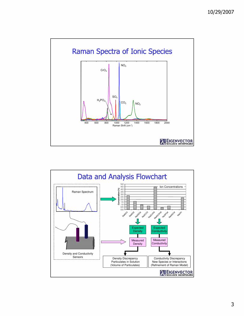
Raman Spectra of Ionic SpeciesRaman Spectra of Ionic Species
400 600 800 1000 1200 1400 1600 1800 2000Raman Shift (cm-1)
NO3
NO2
SO4
CO3
CrO4
H2PO4
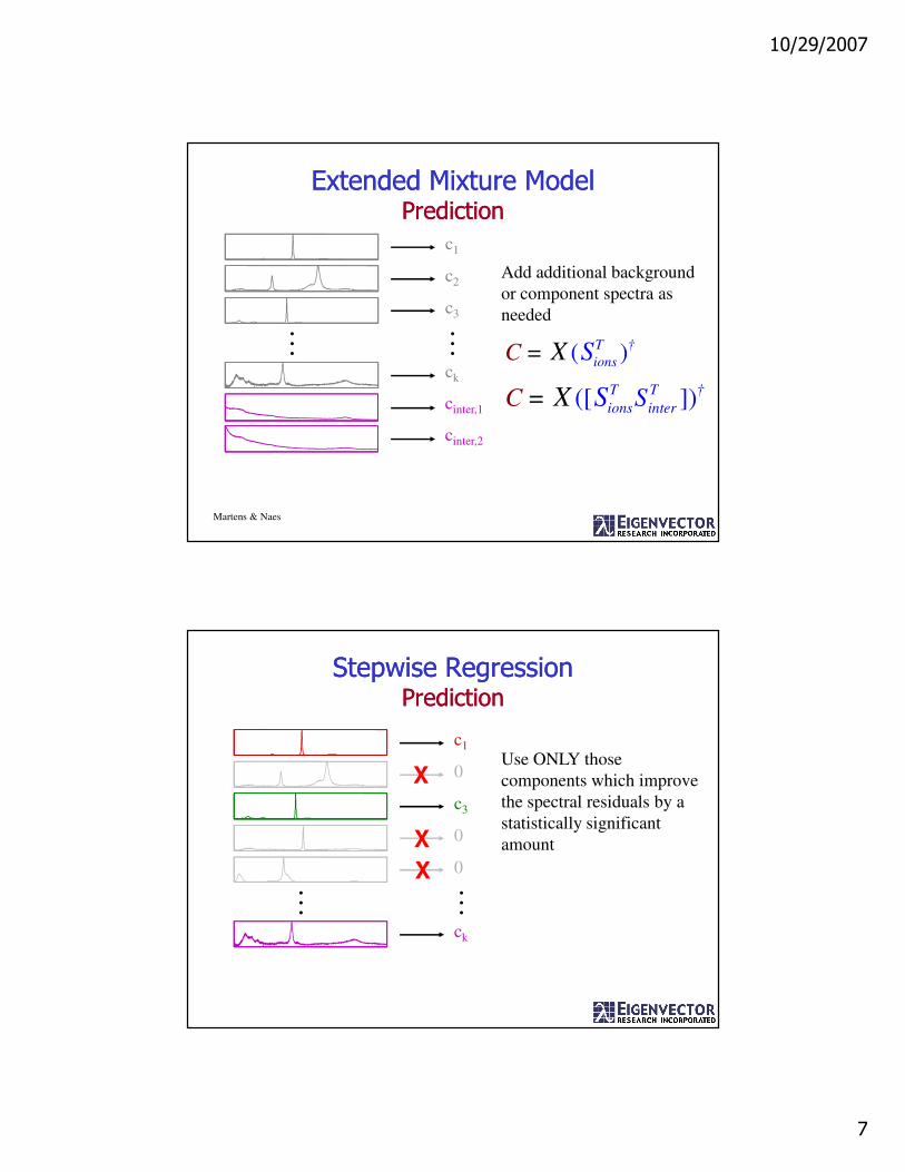
Raman Spectrum
0.0
0.5
1.0
1.5
2.0
2.5
3.0
3.5
4.0
4.5
5.0
Co
ncen
trati
on
(%
) Ion Concentrations
Expected
Density
Expected
Conductivity
Measured
Density
Measured
Conductivity
Density Discrepancy
Particulates in Solution
(Volume of Particulates)
Conductivity Discrepancy
New Species or Interactions
(Refinement of Raman Model)
Density and Conductivity
Sensors
Data and Analysis FlowchartData and Analysis Flowchart

10/29/2007
4
Estimation of Density and Conductivity from Concentrations
(1st generation models)
Estimation of Density and Conductivity from Concentrations
(1st generation models)
(dimmed and/or labeled points were not used in modeling)
50 100 150 200 250 300 3500
100
200
300
400
500
600
700
Measured Conductivity, mS/cmP
redic
ted C
onductivity,
mS
/cm
AlO2-1 AlO2-2
AlO2-3
PO4-4
SiO4-3 SiO4-4
NaOH-1 R
NaOH-2 R
NaOH-3 R
NaOH-4 R
mix-5
mix-11
mix-14
mix-15
mix-22
mix-25
mix-27
mix-29
mix-30
mix-33
mix-34
mix-35
mix-36
mix-37
mix-40
mix-43
1.05 1.1 1.15 1.2 1.25 1.3 1.35 1.41
1.05
1.1
1.15
1.2
1.25
1.3
1.35
1.4
1.45
Measured Density, g/ml
Pre
dic
ted D
ensity,
g/m
l
SiO4-3
SiO4-4
Conductivity
Num. LVs: 4
RMSEC: 0.019RMSECV: 0.021
Density
Num. LVs: 3
RMSEC: 17.4132 RMSECV: 22.9085
Raman-to-Concentration Model Design Challenges
Raman-to-Concentration Model Design Challenges
• Long-Term Model
– Months-Years of Service
• Unknown Field Interferences
– Updates probably necessary

10/29/2007
5
Regression Model OptionsRegression Model Options
• ILS – Inverse Least Squares (PLS, PCR, MLR)
+ Nonlinearities often easily included
- Model updating a challenge
• CLS – Classical Least Squares
+Model updating straightforward
- Does not typically allow for nonlinearities
Classical Least Squares ModelClassical Least Squares Model
As concentration increases, there is a
corresponding increase in intensity as
a linear response (i.e. Beer’s law).
The typical CLS model uses a simple
response profile (spectrum) to predict
concentration of the individual species.0 200 400 600 800 1000
0 20 40 60 80 100
Species Concentration
Frequency
Pure
com
ponent
Spectr
um
pro
jection
Ram
an Inte
nsity
si
ci
T= +X CS E
C
e.g
Time
ST

10/29/2007
6
Standard CLS ModelCalibration
Standard CLS ModelCalibration
T
ions cal
†
cal
T=
= C
CS
XS
X Determine pure component spectra
(ST) from calibration samples by
ordinary least-squares regression.
leastsquares
leastsquares
least
squares
Ccal pure component spectramixtures
Standard CLS ModelPrediction
Standard CLS ModelPrediction
c1
c2
c3
c4
c5
ck
Standard “linear” CLS
Each spectrum maps to
one concentration.
… … ( )T †
ionsC = SX
10/29/2007
7
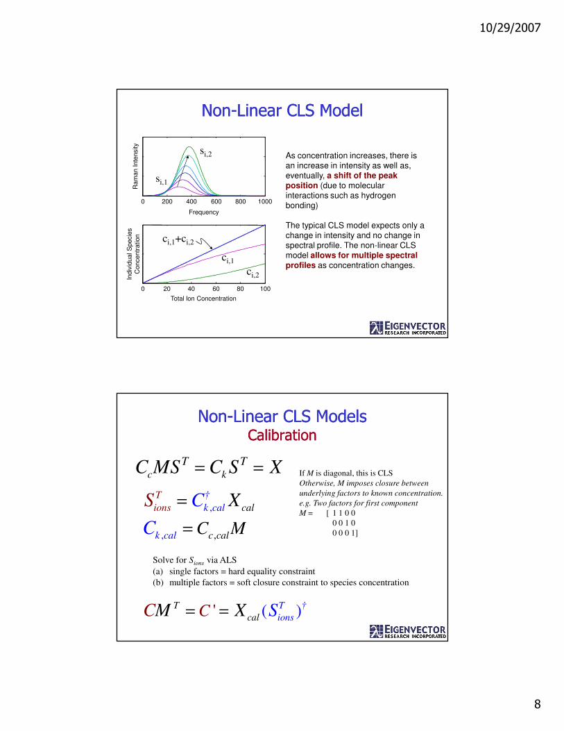
Extended Mixture ModelPrediction
Extended Mixture ModelPrediction
c1
c2
c3
ck
Add additional background
or component spectra as
needed… …cinter,2
cinter,1
Martens & Naes
( )T †
ionsC = SX
([ ])T T †
ions inter= SC SX
Stepwise RegressionPrediction
Stepwise RegressionPrediction
Use ONLY those
components which improve
the spectral residuals by a
statistically significant
amount
c1
0
c3
0
0
ck
… …
X
X
X
10/29/2007
8
Non-Linear CLS ModelNon-Linear CLS Model
As concentration increases, there is
an increase in intensity as well as,
eventually, a shift of the peak position (due to molecular
interactions such as hydrogen
bonding)
The typical CLS model expects only a
change in intensity and no change in
spectral profile. The non-linear CLS
model allows for multiple spectral profiles as concentration changes.
0 200 400 600 800 1000
0 20 40 60 80 100
Total Ion Concentration
Frequency
Indiv
idual S
pecie
s
Concentr
ation
Ram
an Inte
nsity
ci,1+ci,2
ci,1
ci,2
si,1
si,2
Non-Linear CLS ModelsCalibration
Non-Linear CLS ModelsCalibration
c k
T TC MS C S X= =
' ( )T
cal
T †
ionsC SM XC = =
, ca
†
k
T
ion lcalsS XC=
,,k cal c calC MC =
Solve for Sions via ALS
(a) single factors = hard equality constraint
(b) multiple factors = soft closure constraint to species concentration
If M is diagonal, this is CLS
Otherwise, M imposes closure between
underlying factors to known concentration.
e.g. Two factors for first component
M = [ 1 1 0 0
0 0 1 0
0 0 0 1]

10/29/2007
9
Non-Linear CLS ModelPrediction
Non-Linear CLS ModelPrediction
c1
c2
c3
c4
ck
“Non-linear” CLS
More than one pure
component spectrum
can map to an
underlying species
concentration.……
c'1,1
c'1,2
c'1,3
c'2
c'3
c'4
c'k…
0 2 4 6 8-10
-5
0
5
10
NaAl(OH)4
Na
Al(O
H)4
pre
d
0 5 10 150
5
10
Na2CO3
Na
2C
O3
p
red
0 10 20 300
10
20
30
NaNO2
Na
NO
2 p
red
0 10 20 300
10
20
30
NaNO3
Na
NO
3 p
red
0 5 10 15 200
5
10
15
Na2SO4
Na
2S
O4
p
red
0 2 4 60
2
4
6
Na2CrO4
Na
2C
rO4
p
red
0 5 10
0
5
10
Na3PO4
Na
3P
O4
p
red
0 10 20
0
10
20
Na4SiO4
Na
4S
iO4
p
red
Measured Concentration
Estim
ate
d C
on
ce
ntr
atio
n
Classical Least Squares (CLS)
Al(OH)4 in solutionwith NO3

10/29/2007
10
Example: Multiple NO3 ComponentsExample: Multiple NO3 Components
1010 1030 1050 1070 1090
Raman Shift (cm-1)
Normalized spectra at different NO3 concentrations and w/Al(OH)4
increasingionic strength
0 2 4 6 8
0
2
4
6
8
NaAl(OH)4
Na
Al(O
H)4
pre
d
0 5 10 150
5
10
Na2CO3
Na
2C
O3
p
red
0 10 20 300
10
20
30
NaNO2
Na
NO
2 p
red
0 10 20 300
10
20
30
NaNO3
Na
NO
3 p
red
0 5 10 15 200
5
10
15
20
Na2SO4
Na
2S
O4
p
red
0 2 4 60
2
4
6
Na2CrO4
Na
2C
rO4
p
red
0 5 10
0
5
10
15
Na3PO4
Na
3P
O4
p
red
0 10 20
0
10
20
Na4SiO4
Na
4S
iO4
p
red
Measured Concentration
Estim
ate
d C
on
ce
ntr
atio
n
Non-Linear Classical Least Squares (NL-CLS)

10/29/2007
11
Example: Multiple NO3 ComponentsExample: Multiple NO3 Components
Raman Shift (cm-1)
1010 1030 1050 1070 10901010 1030 1050 1070 1090
Raman Shift (cm-1)
Measured Data Recovered Spectra
Normalization of OH2nd DerivativeALS calibration
normalized
increasingionic strength
0 2 4 6 8
0
2
4
6
8
NaAl(OH)4
Na
Al(O
H)4
pre
d
0 5 10 150
5
10
Na2CO3
Na
2C
O3
p
red
0 10 20 300
10
20
30
NaNO2
Na
NO
2 p
red
0 10 20 300
10
20
30
NaNO3
Na
NO
3 p
red
0 5 10 15 200
5
10
15
20
Na2SO4
Na
2S
O4
p
red
0 2 4 60
2
4
6
Na2CrO4
Na
2C
rO4
p
red
0 5 10
0
5
10
15
Na3PO4
Na
3P
O4
p
red
0 10 20
0
10
20
Na4SiO4
Na
4S
iO4
p
red
Measured Concentration
Estim
ate
d C
on
ce
ntr
atio
n
Non-Linear Classical Least Squares (NL-CLS)
Interference of baseline/background
10/29/2007
12
0 2 4 6 8
0
2
4
6
8
NaAl(OH)4
Na
Al(O
H)4
pre
d
0 5 10 150
5
10
Na2CO3
Na
2C
O3
p
red
0 10 20 300
10
20
30
NaNO2
Na
NO
2 p
red
0 10 20 300
10
20
30
NaNO3
Na
NO
3 p
red
0 5 10 15 200
5
10
15
20
Na2SO4
Na
2S
O4
p
red
0 2 4 60
2
4
6
Na2CrO4N
a2
CrO
4 p
red
0 5 10
0
5
10
Na3PO4
Na
3P
O4
p
red
0 10 20
0
10
20
Na4SiO4
Na
4S
iO4
p
red
Measured Concentration
Estim
ate
d C
on
ce
ntr
atio
n
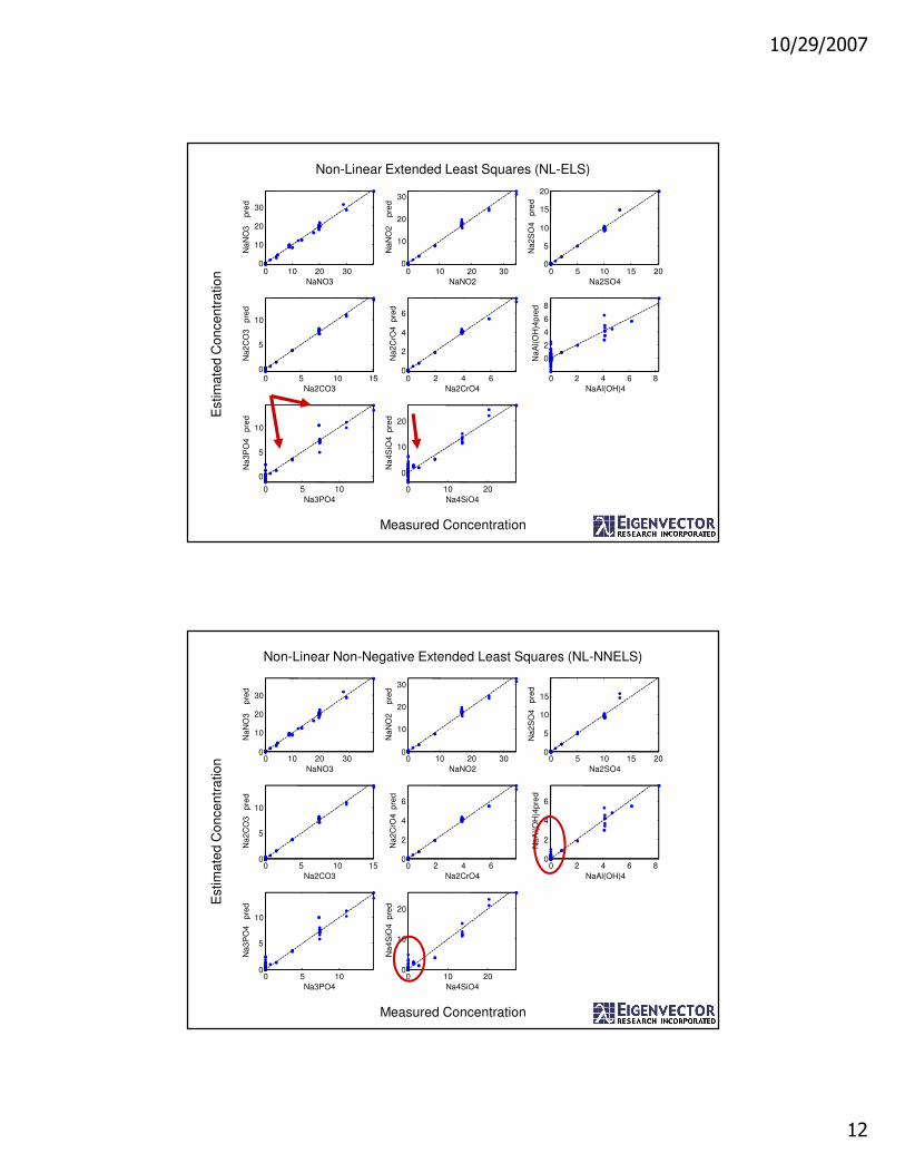
Non-Linear Extended Least Squares (NL-ELS)
0 2 4 6 80
2
4
6
NaAl(OH)4
Na
Al(O
H)4
pre
d
0 5 10 150
5
10
Na2CO3
Na
2C
O3
p
red
0 10 20 300
10
20
30
NaNO2
Na
NO
2 p
red
0 10 20 300
10
20
30
NaNO3
Na
NO
3 p
red
0 5 10 15 200
5
10
15
Na2SO4
Na
2S
O4
p
red
0 2 4 60
2
4
6
Na2CrO4
Na
2C
rO4
p
red
0 5 100
5
10
Na3PO4
Na
3P
O4
p
red
0 10 200
10
20
Na4SiO4
Na
4S
iO4
p
red
Non-Linear Non-Negative Extended Least Squares (NL-NNELS)
Measured Concentration
Estim
ate
d C
on
ce
ntr
atio
n

10/29/2007
13
NO3 NO2 SO4 CO3 CrO4 Al(OH) PO4 SiO4
0.18 0.19 0.36 0.11 0.04 0.43 0.53 0.78 nn
0.19 0.19 0.36 0.09 0.04 0.42 0.48 0.74 sr,nn
0.18 0.19 0.27 0.13 0.04 0.73 0.56 1.25
0.18 0.18 0.36 0.12 0.04 0.61 0.49 1.12 sr
(non-negative basis)
NO3 NO2 SO4 CO3 CrO4 Al(OH) PO4 SiO4
0.26 0.18 0.35 0.10 0.04 0.38 0.48 0.99 nn
0.26 0.18 0.35 0.09 0.04 0.39 0.45 1.04 sr,nn
0.24 0.23 0.34 0.12 0.04 0.43 0.51 0.92
0.24 0.18 0.39 0.10 0.04 0.17 0.44 0.99 sr
Calibration ResultsCalibration Results
Pure samples onlyOH Normalization2nd DerivativeALS calibration for non-linear components
Extended and Non-Linear Models Useful?Ordinary Least Squares
Extended and Non-Linear Models Useful?Ordinary Least Squares
Standard Error of Calibration (SEC)
NO3 NO2 SO4 CO3 CrO4 Al(OH) PO4 SiO4
: 0.60 0.59 0.36 0.24 0.12 3.13 2.24 2.77
B : 0.59 0.61 0.36 0.24 0.12 3.15 1.38 1.70
3: 0.57 0.54 0.31 0.21 0.11 0.61 1.50 2.33
B3: 0.57 0.54 0.31 0.21 0.11 0.67 0.67 1.68
Standard Error of Prediction (SEP)
NO3 NO2 SO4 CO3 CrO4 Al(OH) PO4 SiO4
: 0.53 0.20 0.06 0.21 0.10 2.06 2.26 2.67
B : 0.51 0.21 0.06 0.21 0.10 2.09 1.26 1.49
3: 0.48 0.19 0.12 0.17 0.09 0.55 1.56 2.03
B3: 0.46 0.18 0.13 0.17 0.09 0.58 0.26 1.55
B: Including 2 Background Factors (from NaOH)
3: Non-linear (3 components) for NO3

10/29/2007
14
Extended and Non-Linear Models Useful?Non-negative Least Squares
Extended and Non-Linear Models Useful?Non-negative Least Squares
NO3 NO2 SO4 CO3 CrO4 Al(OH) PO4 SiO4
: 0.56 0.66 0.36 0.49 0.13 2.16 4.83 2.03
BG : 0.60 0.74 0.36 0.45 0.12 1.95 1.65 2.42
NL: 0.56 0.53 0.35 0.20 0.10 0.28 1.49 2.10
BG,NL: 0.56 0.52 0.35 0.20 0.11 0.27 0.61 0.97
NO3 NO2 SO4 CO3 CrO4 Al(OH) PO4 SiO4
: 0.41 0.62 0.06 0.42 0.11 0.55 4.73 1.27
BG : 0.38 1.11 0.11 0.39 0.10 0.62 0.87 0.45
NL: 0.43 0.20 0.07 0.17 0.09 0.31 1.54 1.67
BG,NL: 0.40 0.19 0.12 0.18 0.10 0.20 0.31 0.38
BG: Including 2 Background Factors (from NaOH)
NL: Non-linear (3 components) for NO3
Standard Error of Calibration
Standard Error of Prediction
NO3 NO2 SO4 CO3 CrO4 Al(OH) PO4 SiO4
: 0.57 0.54 0.31 0.21 0.11 0.67 0.67 1.68
SR : 0.56 0.52 0.35 0.20 0.11 0.80 0.61 1.61
NN: 0.56 0.52 0.35 0.20 0.11 0.27 0.61 0.97
SR,NN: 0.56 0.51 0.35 0.19 0.11 0.26 0.53 0.79
SR: Stepwise regression
NN: Non-Negative least squares
Standard Error of Calibration
Standard Error of PredictionNO3 NO2 SO4 CO3 CrO4 Al(OH) PO4 SiO4
: 0.46 0.18 0.13 0.17 0.09 0.58 0.26 1.55
SR : 0.45 0.17 0.13 0.17 0.09 0.55 0.55 1.32
NN: 0.40 0.19 0.12 0.18 0.10 0.20 0.31 0.38
SR,NN: 0.40 0.20 0.12 0.18 0.10 0.22 0.62 0.45
Stepwise and Non-Negative LS Useful?Background + Non-linear NO3
Stepwise and Non-Negative LS Useful?Background + Non-linear NO3
10/29/2007
15
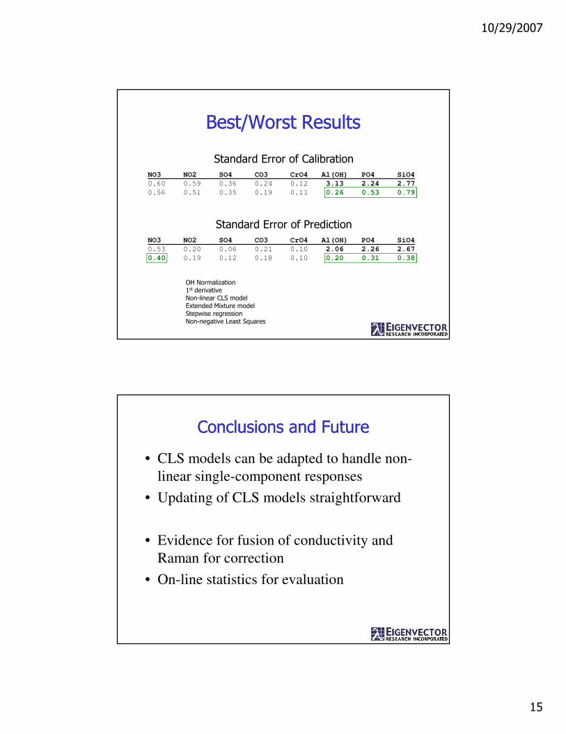
NO3 NO2 SO4 CO3 CrO4 Al(OH) PO4 SiO4
0.53 0.20 0.06 0.21 0.10 2.06 2.26 2.67
0.40 0.19 0.12 0.18 0.10 0.20 0.31 0.38
Standard Error of Prediction
Best/Worst ResultsBest/Worst Results
NO3 NO2 SO4 CO3 CrO4 Al(OH) PO4 SiO4
0.60 0.59 0.36 0.24 0.12 3.13 2.24 2.77
0.56 0.51 0.35 0.19 0.11 0.26 0.53 0.79
Standard Error of Calibration
OH Normalization1st derivativeNon-linear CLS modelExtended Mixture modelStepwise regressionNon-negative Least Squares
Conclusions and FutureConclusions and Future
• CLS models can be adapted to handle non-
linear single-component responses
• Updating of CLS models straightforward
• Evidence for fusion of conductivity and
Raman for correction
• On-line statistics for evaluation