rainfall accumulation and probabilityestimations …
TRANSCRIPT

RAINFALL ACCUMULATION AND PROBABILITY ESTIMATIONS
WITH GEOGRAPHIC INFORMATION SYSTEM
FOR TRANSPORTATION APPLICATIONS
A THESIS SUBMITTED TO THE GRADUATE DIVISION OFTHE UNIVERSITY OF HAWAI'I IN PARTIAL FULFILLMENT
OF THE REQUIREMENTS FOR THE DEGREE OF
MASTER OF SCIENCE
IN
CIVIL ENGINEERING
December 2004
By
Kur-Yi Chang
Thesis Committee:
Dr. Panos Prevedouros (Chairman)Dr. A. Ricardo Archilla
Dr. Edmond Cheng

ACKNOWLEDGEMENTS
The completion of this study was realized with the help by several people. The author
would like to express gratitude to Dr. Panos Prevedouros for being his academic adviser
during his graduate study at the Civil and Environmental Engineering Department of the
University of Hawaii at Manoa. Dr. Prevedouros provided equipment, funding, guidance, and
assistance with the author's research. The author wishes to thank Dr. Ricardo Archilla and
Dr. Edmond Cheng of the Civil and Environmental Engineering Department of the
University of Hawaii at Manoa for being thesis committee members who provided valuable
input and comments on the author's study.
The author wishes to acknowledge Kevin Kodama of NOAA's Honolulu National
Weather Service for providing rainfall information, the Caliper Corporation's Technical
Support for answering Caliper Maptitude related questions, and Dr. Michael Kyte of the
University of Idaho for answering questions about related research.
The author is also thankful to Lin Zhang, Ph.D. candidate in Transportation
Engineering, and James Watson, Master's candidate in Transportation Engineering, for help
during this thesis document compilation.
ll1

ABSTRACT
The study introduces rainfall information estimation with rainfall data from NOAA
and Geographic Information System (GIS) for transportation applications. Application on
signalized intersection operational analysis that accounts for the effects of rainfall was used
to demonstrate the concept.
Three traffic performance parameters of signalized intersections that are likely
affected by rainfall were considered: saturation flow, effective green and progression factor.
Adjusted values for these factors were used to calculate the proposed LOS that accounts for
the effects of rainfall.
Year 2002 monthly rainfall data of all 28 weather observation stations in the City and
County of Honolulu were processed to derive rainfall probabilities during morning and
evening peak hours of traffic. Twelve rainfall probability contour maps were used to estimate
the rainfall probability during peak hours of traffic at any intersection location.
The HCM 2000 procedure for signalized intersection capacity analysis was modified
by combining the proposed Level of Service (LOS) and the rainfall probability.
A case study of five signalized intersections in Honolulu demonstrates the proposed
LOS of signalized intersection that accounts for the effects of rainfall. LOS under the wet
condition lowered by one grade at four out of the five intersections, meaning the traffic
condition is substantially worsened at the intersections. The case study results indicate that
rainfall could have a considerable impact on signalized intersection traffic performance.
The proposed methodology for the application was found feasible and provided
means for accounting for wet conditions in the HCM 2000 capacity analysis procedure.
IV

TABLE OF CONTENTS
ACKNOWLEDGEMENTS iii
ABSTRACT iv
TABLE OF CONTENTS v
LIST OF TABLES vii
LIST OF FIGURES viii
CHAPTER 1 - INTRODUCTION 1
CHAPTER 2 - LITERATURE REVIEW 7
CHAPTER 3 - OBJECTIVES AND METHODOLOGy 13
3.1 Assessment of the Effects of Rainfall on Signalized Intersection LOS 13
3.2 Rainfall Probability Estimation with GIS and Readily Available Data for Any
Intersection Location 15
3.3 Modification to the HCM 2000 Procedure for Capacity Analysis of Signalized
Intersections 18
CHAPTER 4 - DATA PROCESSING AND GIS MAPPING 21
4.1 Data Processing Procedures for Rainfall Probability Estimation 21
4.2 Generating Rainfall Probability Contour Maps with GIS 26
4.3 Rainfall Data Choice Comparison 30
CHAPTER 5 - LEVEL OF SERVICE OF FIVE SIGNALIZED INTERSECTIONS THAT
ACCOUNTS FOR EFFECTS OF RAINFALL 33
5.1 Characteristics of the Intersections 33
5.2 HCM2000 Procedure for Signalized Intersection Capacity Analysis 35
v
5.3 Sample Calculation of the LOS that Accounts for Effects of Rainfall 41
5.4 Analysis Results of Five Signalized Intersections in Honolulu under Dry and Wet
Conditions 45
CHAPTER 6 - SUMMARY AND CONCLUSIONS 48
6.1 Summary 48
6.2 Conclusions 49
6.3 Future Research 50
APPENDIX A - NOAA HYDRONET 51
APPENDIX B - MANUAL FOR GENERATING RAINFALL PROBABILITY CONTOUR
MAPS WITH MAPTITUDE 52
APPENDIX C - SUMMARY OF 2002 OAHU PEAK TRAFFIC HOURS RAINFALL
PROBABILITY 60
APPENDIX D - SAMPLE RAINFALL DATA FILE 62
REFERENCES 63
Vi
LIST OF TABLES
Table 1: Sample Organized Rainfall Data for Morning Peak Period (rainfall
accumulation in inches) 22
Table 2: Sample of Morning and Evening Binary RAIN Variable Cells 23
Table 3: Rain Probability Summary File of the Morning Peak Traffic Hours 24
Table 4: Level of Service Table 41
Table 5: Field Data 43
Table 6: Saturation Flows and Flow Ratios 43
Table 7: Capacity Analysis 44
Table 8: LOS 44
Table 9: Comparison of LOS under Dry and Wet Scenario 3 44
Table 10: Analysis of Five Intersections under Dry and Wet Conditions 47
Table 11: Estimation of Prevailing Delays under Dry and Wet Conditions 47
Vll

LIST OF FIGURES
Figure 1: Flowchart of the Methodology of Estimation of Rainfall Probability during
Peak Traffic Hours with GIS and Readily Available Rainfall Data 17
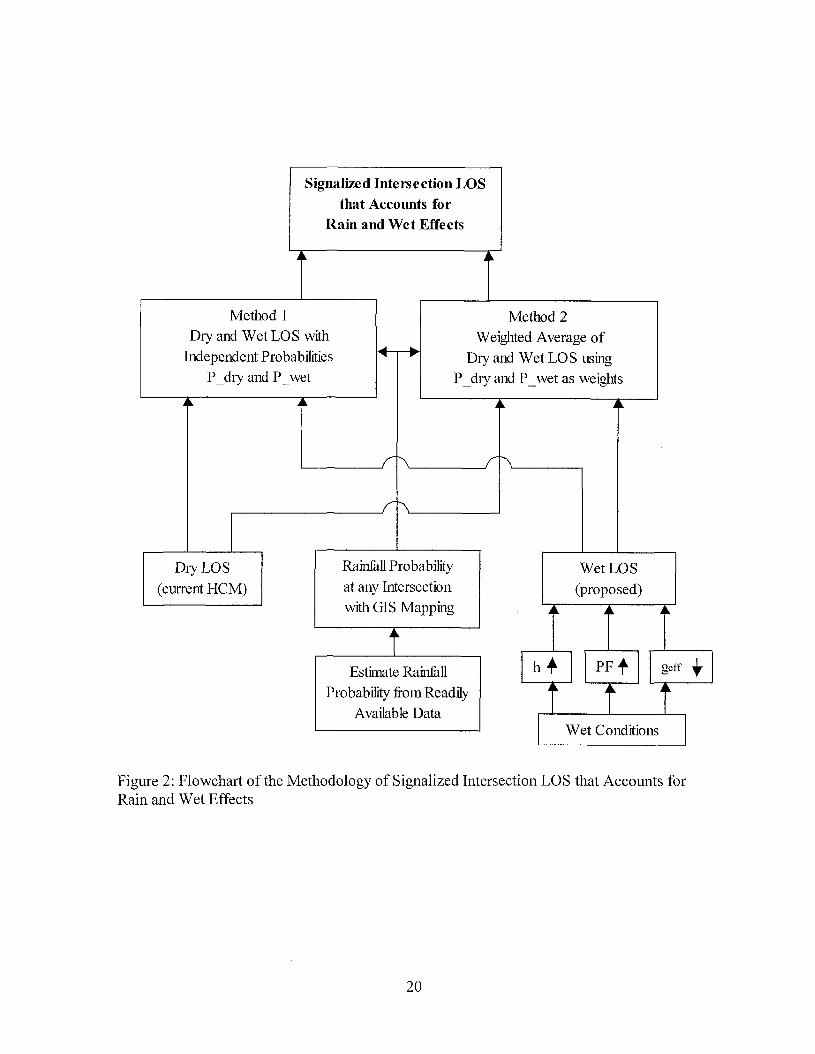
Figure 2: Flowchart of the Methodology of Signalized Intersection LOS that Accounts
for Rain and Wet Effects 20
Figure 3: List of Weather Observation Stations in the City and County of Honolulu 25
Figure 4: Sample rainfall probability contour map, City and County of Honolulu,
Oahu, HI, Morning peak traffic hours, February 2002 28
Figure 5: Sample of Estimation of Rainfall Probability with Maptitude, Punahou Street
and Wilder Street Intersection, City and County of Honolulu, Oahu, HI, Morning
Peak Traffic Hours, July 2002 29
Figure 6: New File Type window 52
Figure 7: Create a Map Wizard window 52
Figure 8: Oahu Base Map without Detailed Roadway Information 53
Figure 9: Open File Window: Input Source File for Detailed Roadway Layer 53
Figure 10: Oahu Base Map with Detailed Roadway Information 54
Figure 11: Open File Window: Input Source File for Rainfall Probability Information
Layer 54
Figure 12: Save File Window: Save Morning Rainfall Probability Information 55
Figure 13: Save File Window: Save Generated Geographic File into Maptitude
Readable Database Format 55
Figure 14: Rainfall Probability Geographic Data, both Table and Graph (upper) 56
Vlll

Figure 15: Layer Window (upper right) 56
Figure 16: Open File Window: Input Morning Rainfall Probability Geographic File
(right) 56
Figure 17: Surface Analysis Window, Settings Tab 57
Figure 18: Surface Analysis Window, Options Tab 57
Figure 19: Contour Layer Window 57
Figure 20: Manual Theme Window 57
Figure 21: Surface Analysis Toolbox with "Calculate Spot Data" Button LabeL 59
Figure 22: Sample of Estimation of Rainfall Probability with Maptitude, Punahou
Street and Wilder Street Intersection, City and County of Honolulu, Oahu, HI,
Morning Peak Traffic Hours, July 2002 59
IX

CHAPTER 1 - INTRODUCTION
Rainfall has various effects on transportation systems. Depending on intensity and
characteristics of the rainfall, the various elements of transportation systems are affected by
rainfall differently. Transportation systems consist of roadway, railroad, pipeline, water
transportation, and air transportation systems. Rainfall effects on each one of them are
discussed in the following paragraphs.
The roadway system, which consists of intersections, local roadways, arterials,
highways, and freeways, is particularly affected by the effects of rainfall. Rainfall affects not
only roadway traffic performance but also the integrity of the roadway infrastructures.
Rainfall impacts roadway traffic performance with three main impedance factors: [1,2,3]
• The presence of a water film on the surface of the pavement
• Reduced visibility and light scattering
• Raindrops, spray, and road grime on vehicle windshields
Rain affects roadways, vehicles, and drivers. The main effects of rain on roadways
are the reduction of friction between tire tread and road surface, and the reduction of
pavement skid resistance. Water film thickness can vary from damp or visibly wet to a depth
of several millimeters. Reduction of pavement skid resistance is a combined result of factors
such as the thickness of water film on the surface, pavement texture, tire-tread depth and
composition, and vehicle speed. When a critical thickness of water film is exceeded,
aquaplaning may occur and tire-road friction is lost. In general, rain decreases vehicle
stability and maneuverability [3].
1

The windscreen and windows of vehicle are covered by raindrops during rain. That
leads to poor visibility. Moreover, splash and spray from other vehicles worsen visibility
problems by adding a film of dirt. Raindrop diameter and concentration correlate with
rainfall intensity. Visibility is reduced with increasing raindrop diameter and intensity of
precipitation [4]. Visibility reduction is mostly attributable to: [1]
• The combined effect of a screen of rain and light causes bright and scattering
light affecting the visual perception ofdrivers.
• The drops and windscreen glass create unbalanced lenses reflecting light into
driver eyes. The surface of drops also scatters light.
The problem of visibility reduction is more severe when rain occurs at night [1]. The
overall effect of rain on drivers is poor visibility and object recognition. Drivers may try to
maintain longer distances between vehicles and drive at slower speeds to account for the
longer perception/reaction time and stopping distance during rain. These lead to longer travel
times and more congestion on the roadways. While the effects of rainfall on individual
vehicles may be limited, the effects on the entire roadway network are likely exponentially
amplified.
In addition to the effects of rainfall itself, excessive accumulation of rainfall on
roadways can cause serious disruption to roadway traffic performance. A significant portion
of the cost of most roadway systems is attributable to drainage facilities, such as storm
drains, highway culverts, bridges, and other water control structures [6].
Other than the effects on roadway traffic performance, rainfall has long been
recognized as a factor to the deterioration of roadway pavement structures. It affects both
2

pavement surface and subgrade. Rainfall contributes to the generation of roadway
deteriorations such as potholes, cracks, raveling, and rutting. The negative effects of roadway
deterioration range from discomfort and unpleasant driving experience for drivers and
passengers to being a contributing factor to traffic accidents.
For railroad and pipeline systems, rainfall can cause subgrade deterioration.
Depending on severity of the rainfall and quality of the engineering design, deterioration can
lead to railroad and pipeline system disruptions ranging from minor repairs to catastrophes,
such as derailing of trains due to unexpected subgrade structure failures. In addition, roadway
and railway transportation are also affected by precipitation (water or snow) indirectly but
severely because extended waterfall or snow accumulation lead to land slides and
avalanches, respectively.
Rainfall has minimum effects on water and air transportation systems, unless it is of
extreme rainfall condition such as hurricane and thunderstorm. However, rainfall is a concern
for air travel safety. Since airplanes need to land and take-off from airport runways, the
presence of a water film from rainfall reduces friction between airplane tires and runway
surface.
Although rainfall has various effects on transportation system, as described above,
effects of rainfall are not fully considered in most of the transportation design and operation
guidelines.
The Highway Capacity Manual 2000 (HCM 2000), which is the national standard for
roadway systems operational analysis, states that "Base conditions assume good weather,
good pavement conditions, users familiar with the facility, and no impediments to traffic
flow." [6] However, it is commonly perceived by the motorists that rainy conditions increase
3

traffic congestion and cause longer travel times. The current design and analysis procedures
do not necessarily reflect the average driving conditions experienced by the motorists.
Pavement design guideline accounts for the effects of traffic, subgrade, reliability,
drainage, and construction considerations, but not for the effects of rainfall. Good drainage
and subgrade designs can lessen the effect of rainfall but not eliminate the effects of rainfall.
While the effects of rainfall are significant and broad on transportation systems, the
lack of consideration for the effects of rainfall is probably due to difficulties in doing so. It
simply was not possible to gather all of the required information, organize it, conduct
computations, and prepare presentations without involving on excessive amount of effort.
The development in computer tec1mologies and the flourishing of the Internet in the past
decades are the most important factors that make the incorporation of rainfall effects into the
designs of transportation systems possible today. For example, widely available powerful
computer processors, large data storage devices, and data access via the Internet has made
possible the analysis of large amounts of rainfall accumulation data.
Estimation of rainfall information with GIS and readily available data is now an
economical and convenient alternative without difficult and expensive undertakings with
weather observation stations.
Estimation of rainfall information with GIS and readily available data can be used for
many transportation applications. A list of possible applications is stated below:
• Estimation of rainfall volume for roadway system drainage design
• Evaluation of rainfall effects on roadway pavement design and maintenance
• Evaluation of rainfall effects on pipeline and railroad design and maintenance
4

• Analysis of land slides, avalanches, and flush floods that may threaten
transportation infrastructure.
• Assessment of rainfall effects on roadway system (including intersection,
roadway, highway, and freeway) traffic performance
Estimation of rainfall volume for roadway system drainage design is important,
because, as mentioned, a significant portion of the cost of most roadway system is
attributable to drainage facilities. In 1998, Olivera and Maidment used GIS in hydrologic
data development for design of highway drainage facilities [5]. Even though the Texas
Department of Transportation (TxDOT) had existing computerized procedures for hydrologic
and hydraulic analysis in the TxDOT Hydrologic and Hydraulic System (THYSYS), each
application required the digital description of the watershed and the stream channel using
data extracted manually from maps and cross sections contained in drawings. The process
was tedious and troublesome. Olivera and Maidment's study integrated spatial data
describing the watershed with hydrologic theory. That led to the reduction of analysis time
and the improvement of accuracy for the design of highway drainage facilities in Texas.
Evaluation of rainfall effects on roadway pavement helps researchers and engineers to
improve roadway pavement durability. Even though now there is porous pavement design
that can already improve pavement drainage and provide safer driving condition under the
rain, inexpensive alternative way to collect field rainfall data along roadway that can be used
for roadway maintenance purpose is still worth study.
Among all the possible applications of the concept, this study focuses on the use of
readily available rainfall data, estimation of rainfall probability, and the subsequent input into
5

GIS in the calculation of Level of Service (LOS) of signalized intersection that accounts for
effects of rainfall. It intends to demonstrate the value and feasibility of rainfall information
estimation with GIS for transportation applications.
The materials of this study are presented in the following manner. Chapter 2 describes
past studies about the effects of rainfall on roadway traffic performance. Chapter 3 describes
the objectives and the methodology of this study. Chapter 4 explains the data processing and
GIS mapping procedures of this study in details. Chapter 5 demonstrates the calculation
procedures of the LOS that accounts for the effects of rainfall on five signalized intersections
in Honolulu. Chapter 6 concludes the study with the summary and conclusions.
6

CHAPTER 2 - LITERATURE REVIEW
Rainfall intensifies traffic congestion and increases travel time. Past studies about the
effects of rainfall on traffic performance indices were researched. Research about the effects
of weather on signalized intersection traffic performance is at its infancy. Only two studies
relate to the effects of rainy and wet conditions at signalized intersection are available.
Martin et al. reported in 2000 about their research on arterial street operations under
inclement weather conditions [7]. Traffic data was collected from two intersections.
Saturation flows were obtained with automated traffic data collectors. Speeds were collected
using radar guns. The saturation flow and speed data were obtained on dry weather days and
14 different inclement weather days over winter 1999 - 2000. Weather was categorized into
seven conditions: normal/clear, rain, wet and snowing, wet and slushy, slushy in wheel paths,
snowy and sticking, and snow packed surface. Average speed decreased about 10% in the
rain. Rain caused a reduction in saturation flow of about 6%. The average start-up lost time
increased from 2.0 seconds to 2.1 seconds. Longer headway, slower speed, and decreased
acceleration rate were the main reasons for the reduction in saturation flow.
Agbolosu-Amison reported in 2004 about research on the impact of inclement
weather on traffic performance at a signalized intersection in northern New England. [8] The
weather and road surface conditions were categorized into six different classes (dry, wet, wet
and snowy, wet and slushy, slushy, and snowy and sticky), and values for the saturation
headways and startup lost times were collected for each weather condition. Saturation
headway was found to be 2% to 3% longer in wet conditions. Start-up lost time was found to
7

be 8% to 10% longer in wet conditions. That is roughly equal to 0.2 seconds in 2.3 seconds
average start-up lost time.
Two studies alone are insufficient to verify the effects of rainfall on traffic
performance. Research about the effects of weather on highway and freeway traffic
performance is presented below.
Kockelman reported in 1998 about her investigation that weather conditions, driver,
and vehicle population characteristics affect the flow-density relationship of a homogeneous
roadway segment [9]. Data were obtained from the Freeway Service Patrol Project from
paired loop detectors on a 5-lane section ofI-880 in Hayward, California. Weather data was
obtained from a variety of sources such as newspaper reports and NOAA reports. Rainfall
intensity was not considered: days were either "rainy" or "dry." Kockelman concluded that
rain could have a statistically significant influence on the flow-density relationship.
Holdener reported in 1998 about the effect of rainfall on freeway speed and capacity
using data from U.S. 290 freeway in Houston, Texas [10]. Rainfall had a significant impact
on speeds. Wet conditions caused a drop in speed from 0.2 to 37.9 km/h (0.12 to 23.6 mph)
with an average speed drop of 13.9 km/h (8.6 mph) when traffic volume was at or near
capacity during the afternoon peak period. A speed drop of 10.7 to 16.3 kmlh (6.7 to 10.1
mph) with an average speed drop of 13.1 km/h (8.1 mph) occurred when the volume was
low, during midday. Wet conditions were estimated to cause a capacity reduction of about
8% to 24%.
FHWA's Weather Management web site [11] contains comprehensive summaries of
the effects of weather on traffic systems, but sources for the information are not cited. The
site reports the following impacts of weather effects on roadway traffic performances:
8

• Freeways: light rain reduces speed by roughly 10%, decreasing capacity by
approximately 4%.
• Freeways: heavy rain decreases speed by about 16%, lowering capacity by
roughly 8%.
• Arterials: rain reduces speed by 10% and capacity by 6%.
The HeM 2000 states that speeds are not particularly affected by wet pavement until
visibility is also affected [12]. This suggests that light rain does not have much effect on
speeds (and presumably not on flows) unless it is of such extended duration that there is
considerable water accumulation on the pavement. Heavy rain, on the other hand, affects
visibility immediately and can be expected to have a noticeable effect on traffic performance.
This expectation is borne out by studies of freeway traffic. Research found minimal
reductions in maximum observed flows for light rain but significant reductions for heavy rain
[13]. Likewise, the research found a small effect on operating speeds for light rain and larger
effects for heavy rain. These changes in operating speeds are important because they directly
affect traffic performance.
For light rain, a reduction in free-flow speeds of 1.2 mi/h was observed [13]. At a
flow rate of 2,400 veh/h, the effect of light rain was to reduce speeds to about 51 mi/h,
compared with speeds of 55 to 59 mi/h under clear and dry conditions. Under light rain
conditions, little if any effect was observed on flow or capacity. For heavy rain, the drop in
free-flow speeds was 3 to 4 mi/h. The result of heavy rain is to reduce speeds, at 2,400 veh/h,
to 47 and 49 mi/h from, respectively, 55 and 59 mi/h. These are reductions of 8 and 10 mi/h,
9

or reduction of 14% and 16%. Maximum flow rates can also be affected and might be 14 to
15 % lower than those observed under clear and dry conditions.
In 2001, Kyte et al. reported research about the effect of environmental factors on
free-flow speed [14]. The estimation of free-flow speed is an important part of the process of
determining the capacity and level of service for a freeway. Data for the study were collected
by visibility and roadway sensors installed on a segment of 1-84 in southeastern Idaho in
1995. The data were collected to examine traffic flow rates and driver speeds during periods
of reduced visibility and other hazardous driving conditions.
The study found that driver speeds drop by more than 14 kmlh from normal condition
when visibility drops to less than 0.1 mile or 160 meters. Heavy rain caused a drop in speed
of about 31.6 km/h (19.6 mph). A best-fit model was developed that included three variables:
wind speed, precipitation intensity, and pavement conditions:
speed = 126.52 - 9.03 x WS - 5.43 x PC - 8.74 x R
where,
(45.05) (A.43) (-7.70) (-13.73) t statistic of the coefficient
speed = prevailing average vehicle speed in km/h
WS = wind speed in two levels, 1 for WS ~ 48 km/h, 2 for WS ~ 48 km/h
PC = pavement condition with three levels, 1 = dry, 2 = wet, 3 = snow/ice
R = rain intensity with 4 levels, 1 = none, 2 = light, 3 = medium, 4 = heavy
10

A disadvantage of models with parameters such as PC and R is that they automatically imply
a specific and linear change for each level of the categorical variable, e.g., snow/ice is three
times worse than dry, whereas in reality is may be many times more or less worse that dry.
The combination of either light or medium precipitation and high wind speeds
reduces mean speeds ranged 24 to 27 km/h from that of the normal condition of 109 km/h.
That roughly equals to 22% to 25% in reduction. Comparing to 14% to 16% reduction
suggested by the HCM 2000, Kyte's et al study suggests that the effect oflight rain and
heavy rain could be 50% higher than what is stated in the HCM 2000.
Prevedouros' et al. analysis of 127 four-hour videotapes recorded between 1996 and
2000 from freeway and arterial surveillance cameras in Honolulu focused on measurements
from traffic platoons ranging in size between 6 and 61 vehicles with an average platoon size
of 12 vehicles [15]. Data were collected during busy but fluid conditions and headways were
measured at identical locations under dry conditions (680 platoons), wet pavement but no
rain (436 platoons) and light-to-moderate rain conditions (388 platoons). The mean headway
(h) for dry conditions was 1.69. The mean h for rain and wet conditions were 1.76 and 1.77
sec., respectively. A linear regression model was developed for arterial streets.
h = 1.411 + 0.052 G + 0.056 R + 0.448 W
where,
h = headway in sec.
G= grade in %
R = rainy or wet conditions, 1 = rain/wet, 0 = dry
W = weekend day, 1 = weekend or holiday, 0 = normal work day
11

The model indicated that weekday rush hour headways are much shorter (1.47 sec.)
than weekend and holiday headways (1.86) and about 4% longer in wet or rainy conditions.
From the past studies, the effects of rainfall on traffic performance can be
summarized:
• Headway is longer by 2% to 5%
• Capacity is lower by 4% to 24%
• Start-up lost time is longer by 0.1 to 0.2 seconds
• Speed is reduced by 10% to 25%
With the effects of rainfall on roadway traffic performance verified from the past
studies and the lack of consideration for the effects of rainfall on signalized intersection in
the current assessment method identified, the concept of Level of Service for signalized
intersection that accounts for effects of rainfall was proposed.
12

CHAPTER 3 - OBJECTIVES AND METHODOLOGY
The objective of this study is to use GIS and readily available rainfall data to
calculate the probability of wet conditions at any location on a map and then use this
probability in the traffic performance assessment of signalized intersection that accounts for
the effects of rainfall. The proposed assessment method is based on the current HCM 2000
procedure for signalized intersection Level of Service (LOS) analysis.
LOS describes the quality of operational conditions within a traffic stream. LOS of
signalized intersection is based on control delay per vehicle [6]. Delay is categorized into A
to F grades with respective delay range for each grade. While A to D indicates that the
intersection traffic conditions are acceptable, E and F indicate unacceptable traffic
conditions. Details about the LOS calculation are explained in Section 5.2.
To achieve the objective, a set of methodology was developed for this study. The
proposed methodology consists of three components:
1. Assessment of the effects of rainfall on signalized intersection LOS.
2. Rainfall probability estimation with GIS and readily available data for any
intersection
3. Modification of parameters in the HCM 2000 procedure for capacity analysis on
signalized intersection to account for effects of rainfall.
3.1 Assessment of the Effects of Rainfall on Signalized Intersection LOS
Three traffic performance factors are likely to be affected by rainfall:
• Headway (h)
13

• Effective Green (gejJ)
• Progression Factor (PF)
Headway is the time elapsed between two consecutive cars on the road, counting
between the same locations (e.g. head to head) of the two cars, usually presented in seconds.
Headway is likely to increase because driver's perception and reaction time is longer in the
rain and motorists tend to think braking is less effective on wet pavement. Motorists keep
longer distance between vehicles to compensate for these for safety reason.
Effective green can be explained with the equation below:
gefl = g - (Start - up lost time) - (Y + AR utilization)
Effective green is the time of green light minus start-up lost time plus yellow and all red
utilization time. Start-up lost time is the time required for the motorist to perceive, react, and
accelerate from the stop line after the traffic signal changes from red to green. Yellow and all
red utilization is the time after traffic signal changes from green to yellow and even red but
cars still run through the intersection. Even though it is not particularly safe for the motorists,
it increases traffic flow through the intersection.
Effective green is likely to decrease because start-up lost time at intersection is longer
and clearance interval, yellow and all red (Y+AR), utilization is likely to be less as motorists
become more conservative in the rain.
Traffic progression is likely to worsen because the normal traffic pattern that is
assumed coordinated is disturbed by the rain (due to slower speed, longer headway, etc.).
Therefore, Progression Factor will likely increase. Higher value for the Progression Factor
means more delay. However, the effects of progression deterioration are largely limited to
14

the through movements only. Traffic signals for turning movements are not normally
coordinated with cross road downstream signals.
These changes in driver behavior could be compensated by traffic-adaptive signals,
but common pre-timed and actuated signals with stop line detection cannot make adequate
adjustments. Therefore, these three behavioral changes of drivers may impose important
impacts on signalized intersection LOS.
3.2 Rainfall Probability Estimation with GIS and Readily Available Data
for Any Intersection Location
Developing estimates for rainfall probability requires a considerable effort to screen
and summarize rainfall data during peak hours of traffic. For this study, monthly rainfall data
for year 2002 from 28 available weather observation stations in the City and County of
Honolulu were manually processed to derive rainfall probability information during peak
hours of traffic.
The procedure was divided into two parts: "Estimate Rainfall Probability with
Readily Available Data" and "Rainfall Probability at any Intersection with GIS Mapping."
"Estimate Rainfall Probability with Readily Available Data" consists of steps
necessary to obtain rainfall probability during peak hours of traffic for signalized intersection
LOS that accounts for effects of rainfall with readily available data. Rainfall probability of
peak hours of traffic is used because rainfall imposes the most significant influence on
signalized intersection traffic performance when intersection reaches capacity or near
capacity. In this study, peak hours of traffic refer to 7-9 AM morning peak hours and 4-6 PM
evening peak hours.
15

To estimate rainfall probability, raw rainfall data are necessary. Raw rainfall data
from Honolulu "Hydronet" of the National Weather Forecasting Office of the NOAA were
used for this study. "Hydronet" was chosen as the data source for its accuracy and recording
interval (IS-min interval) [16]. Because the purpose of this procedure is to find rainfall
probability during peak hours of traffic, rainfall data with short interval, such as IS-min
interval, is preferred.
Once the appropriate rainfall data are found and extracted from the NOAA website,
headers and labels are added to the files for better readability. Data of peak hours of traffic
are highlighted and binary RAIN functions are inputted to identify trace of rainfall during
peak hours of traffic. Rainfall probabilities are then calculated. Details are described in
Chapter 4.
"Rainfall Probability at any Intersection with GIS Mapping" consists of steps that
estimate rainfall probability at any intersection within rainfall contour map with GIS.
The findings of rainfall probabilities from "Estimate Rainfall Probability with
Readily Available Data" are summarized into a single file, and then the file is inputted to a
GIS program to generate rainfall probability contour maps. With GIS ability to spot estimate
interpolated rainfall probability value from the rainfall probability contour maps, rainfall
probability at any intersection within the contour range can be estimated.
The probability of wet conditions and its corresponding dry conditions are then
available for the modification of the HCM procedure for capacity analysis on signalized
intersection as stated in the previous section. Detailed procedures for five signalized
intersections are described in Chapter 5. The process is illustrated in the Figure 1 flowchart.
16

Estimate RainfallMonthly Probability with
NOAA dataReadily Available Data
1Choose year and month I
(Files of all stations Iin one ziDDed file)
~Import into a spreadsheet
program name bystation_month-year
Rainfall Probability at(e.g. Manoa_Jan_2002)
~any Intersection with
GIS Mapping
I
Insert
Idate (columns)& time (rows)
1I Manual highlight ~ I
AM peak period (7-9 AM)PM peak period (4-6 PM)
1Import the rainfalll
probability file into aGIS program
ICalculate rainfall in I 1AM, PM peakperiods
IAdd Layer of P_RAIN
I1 I Add layer of morning or
II Introduce binary RAI~ I evening peak hours rainfallvariable (0,1) for days nrobabilitv
with rainfall> 0.00 ...1 Choose month I
--rI Sum up RAIN = 1 to finddays with rainfall in each
I
Generatemonth and AM PM Deriod P_RAIN_MORNING or
1 EVENING contour layer
Estimate probability for rainyconditions I Zoom into I I
Repeat thetarget location
pm =~W!1I1JRAIN),y_process for
fWN Days in Month ---. another month of
SUM(RAIN),u the year or Use "Spot Elevation"J~~~N
Days in Month another station function to estimateP_RAIN at target
1location
Generate AM, PM summary sheets with- station names, coordinates Use derived
- rainfall probability of each month/station probabilities in- average, max, min per station signalized intersection
1analysis
I(e.g.
Output file: , IP RAIN SUM yearP_RAIN_SUM_2002.xLS)
I
I
Figure 1: Flowchart of the Methodology of Estimation of Rainfall Probability during PeakTraffic Hours with GIS and Readily Available Rainfall Data
17

3.3 Modification to the HCM 2000 Procedure for Capacity Analysis of
Signalized Intersections
The proposed modification to the HCM 2000 procedure for capacity analysis of
signalized intersection that accounts for the effects of rainfall is illustrated by the flowchart in
Figure 2. This bonds everything mentioned in the study together.
In the proposed modification, the capacity analysis of signalized intersection is
executed twice: once with inputs for prevailing saturation flow, effective green and
progression factor, based on dry conditions and a second time with headway increase by a%,
effective greens decreased by ~ seconds and progression factors worsened by y% considered.
The values of parameters a, ~, and yare critical, and reliable values of the parameters are
expected to be determined by future research.
The probabilities of dry and wet conditions are needed in order to estimate the
average prevailing and wet conditions. Since rainfall imposes the most significant impact on
traffic performance during peak hours of traffic and peak hour analysis is required by the
HCM 2000, the probability of rainfall during peak hours of traffic is estimated and
emphasized in this study. After probabilities are estimated, the delays under dry and wet
conditions and the probabilities can be inputted to two alternative methods of signalized
intersection performance assessment. The first method is more suitable for assessment of a
single intersection. The second method is more suitable for comparison between
intersections.
The first method states LOS and delay of dry and wet condition independently with
their respective probability. For example, LOS and delay of dry and wet conditions with
18

respective probability for the intersection of Dole Street and University Avenue may be
stated as:
LOS (Delay) in dry condition = D(54sec.) @ 70% probability
LOS (Delay) in wet condition = E (68 sec.) @ 30% probability
The second method combines LOS and delay of dry and wet conditions into a
weighted average by using probabilities as weights. For example, weighted average LOS and
delay for intersection of Dole Street and University Avenue may be stated as:
Weighted Average LOS (Delay) = E (58.2 sec.) = 54sec.xO.7 + 68sec.x0.3
The weighted average can then be compared with weighted averages of other intersections to
prioritize of intersection improvement projects that are rainfall related. The process is
illustrated in the Figure 1 flowchart.
19
Signalized Intersection LOSthat Accounts for
Rain and Wet Effects
..
Method 1
Dry and Wet LO S with
Independent Probabilities
P_dry and P_wet
..
Method 2Weighted Average of
Dry and Wet LO S using
P_dry and P_wet as weights
..
'----__----J1 \'-__---J( \'---__-,
r----------J1 \'--------'
Dry LOS
(current HCM)
Rainfull Probability
at any Intersection
with GIS Mapping
tEstimate Rainfall
Probability from Readily
Available Data
Wet LOS
(proposed)
I h" I I PF t II geff t I
tI Wet Conditions I
Figure 2: Flowchart of the Methodology of Signalized Intersection LOS that Accounts forRain and Wet Effects
20

CHAPTER 4 - DATA PROCESSING AND GIS MAPPING
With conceptual part of this study explained in the first three chapters, this chapter
describes how the procedures of data processing and rainfall probability estimation with GIS
at any intersection in the City and County of Honolulu can be applied in details. Procedures
stated in this chapter were finalized after many revisions and modifications.
Three types of software were used in this study:
• An Internet browser was used for accessing and downloading rainfall data from
online sources, such as NOAA Hydronet web site. Microsoft's Internet Explorer was
used in this study.
• A Spreadsheet program was used for organizing, manipulating, and analyzing the
rainfall data and preparing input files for GIS. Microsoft's ExceFM was used.
• A GIS program, Caliper's Maptitude™, was used to develop rainfall probability
contours that could be overlaid onto a street map of a given county. Maptitude was
chosen for this task due to its low cost and adequate functionalities.
4.1 Data Processing Procedures for Rainfall Probability Estimation
The basic steps for rainfall probability estimation are illustrated in Figure 2 in
Chapter 3. This section discusses how the data processing was completed.
(1) For the estimation of rainfall probability, rainfall data from "Hydronet" of the
Honolulu office of the National Weather Forecasting Office of the NOAA were used.
Rainfall information on the "Hydronet" is categorized by metropolitan areas, so the name of
21

the metropolitan area is entered to locate the city or county of interest. The City and County
of Honolulu was used for this study.
(2) Database files of a chosen county, month and year, were downloaded and opened in
Microsoft Excel for processing. Since the raw rainfall data is not reader-friendly, column and
row headers for ease of data identification were added. The rainfall data for morning peak
period, as shown in Table 1, were highlighted manually. The rainfall data for the afternoon
peak period were highlighted manually, as well (not shown).
Wet Days l·Jul 2·Jul 3·Jul 4·Jul 5·Jul 6-Jul 7·Jul 8·Jul 9·Jul 10-Jul0:15 68.67 69.67 70.39 70.6 70.65 70.75 70.9 71.9 72.54 73.140:30 68.67 69.67 70.39 70.6 70.65 70.75 70.9 71.9 72.54 73.150:45 68.67 69.67 70.42 70.6 70.65 70.75 70.9 71.9 72.54 73.151 :00 68.67 69.67 70.43 70.6 70.65 70.75 70.9 71.9 72.54 73.181 :15 68.68 69.67 70.43 70.6 70.65 70.75 70.9 71.9 72.54 73.181 :30 68.68 69.67 70.43 70.6 70.65 70.75 70.92 71.9 72.54 73.181 :45 68.72 69.67 70.43 70.6 70.65 70.75 70.94 71.9 72.54 73.182:00 68.75 69.68 70.43 70.6 70.65 70.75 70.95 71.9 72.66 73.182:15 68.76 69.68 70.43 70.6 70.65 70.75 70.95 71.9 72.75 73.22:30 68.8 69.68 70.43 70.6 70.65 70.75 70.95 71.91 72.77 73.252:45 68.81 69.68 70.43 70.6 70.65 70.75 70.95 71.98 72.79 73.263:00 68.81 69.71 70.43 70.6 70.65 70.75 70.95 72.01 72.79 73.273:15 68.81 69.73 70.43 70.6 70.65 70.75 70.97 72.11 72.81 73.293:30 68.81 69.77 70.43 70.6 70.65 70.75 71 72.15 72.82 73.293:45 68.84 69.78 70.43 70.6 70.65 70.75 71.02 72.19 72.88 73.324:00 68.85 69.78 70.43 70.6 70.65 70.75 71.03 72.19 72.93 73.324:15 68.9 69.8 70.43 70.6 70.65 70.75 71.06 72.19 72.94 73.334:30 68.94 69.83 70.43 70.6 70.65 70.75 71.13 72.19 72.94 73.334:45 68.94 69.92 70.43 70.6 70.65 70.75 71.14 72.19 72.94 73.335:00 68.95 69.92 70.43 70.6 70.65 70.75 71.16 72.22 72.94 73.335:15 68.97 69.95 70.43 70.6 70.65 70.75 71.16 72.25 72.94 73.335:30 69 69.95 70.43 70.6 70.65 70.75 71.16 72.25 72.94 73.335:45 69 69.97 70.43 70.6 70.65 70.75 71.16 72.29 72.94 73.336:00 69 70.02 70.43 70.6 70.65 70.75 71.16 72.29 72.95 73.356:15 69 70.09 70.43 70.6 70.65 70.75 71.16 72.29 72.95 73.366:30 69.04 70.12 70.43 70.6 70.65 70.75 71.16 72.29 72.95 73.46:45 69.06 70.14 70.43 70.6 70.65 70.75 71.16 72.29 72.95 73.47:00 69.08 70.16 70.43 70.6 70.65 70.75 71.16 72.3 72.95 73.47:15 69.08 70.16 70.43 70.6 70.65 70.75 71.16 72.3 72.95 73.437:30 69.08 70.16 70.43 70.6 70.66 70.75 71.16 72.3 72.95 73.447:45 69.09 70.16 70.43 70.61 70.74 70.75 71.19 72.31 72.95 73.448:00 16 69.11 70.17 70.43 70.61 70.74 70.75 71.2 72.36 72.95 73.448:15 69.12 70.17 70.43 70.61 70.74 70.75 71.2 72.37 72.95 73.448:30 69.12 70.18 70.43 70.61 70.74 70.75 71.2 72.37 72.95 73.458:45 69.14 70.18 70.43 70.61 70.75 70.75 71.2 72.37 72.95 73.479:00 69.14 70.18 70.43 70.61 70.75 70.75 71.2 72.37 72.95 73.479:15 69.14 70.18 70.43 70.61 70.75 70.75 71.2 72.37 72.95 73.59:30 69.15 70.18 70.43 70.61 70.75 70.83 71.2 72.37 72.95 73.59:45 69.15 70.18 70.43 70.61 70.75 70.83 71.2 72.37 72.95 73.5
10:00 69.21 70.18 70.43 70.61 70.75 70.83 71.2 72.37 72.95 73.5
Table 1: Sample Organized Rainfall Data for Morning Peak Period (rainfall accumulation ininches)
22

(3) Binary RAIN variables are created for morning and evening periods at the bottom of
each column. An equation that subtracted the first cell of the peak period from the last cell of
the peak period is developed. If the result is greater than 0.00, this means that there is at least
a trace of rainfall during this peak traffic period, so "I" shows in the binary RAIN cell. If the
result is 0.00, this means that there is no trace of rainfall during this peak traffic period, so
"0" shows in the cell. The format of the equation is shown below:
IF((last 15 - min rain volume of the peak period -
first 15 - min rain volume of the peak period) > 0,1, 0)
This process is repeated for every day of the month. Table 2 shows morning rain and
afternoon rain binary variable cells for the Waimanalo station for January 2002:
23:15 11.18 11.18 11.19 11.2 11.21 11.25 11.25 11.2823:30 11.18 11.18 11.19 11.2 11.21 11.25 11.25 11.2823:45 11.18 11.18 11.19 11.2 11.21 11.25 11.25 11.28
0:00 11.18 11.18 11.19 11.2 11.21 11.25 11.25 11.28
morning rainevening rain
Waimanalo
days observ. I interval Imin/hour I31 96 I 15 I 60 I 744 I hours I
days I days I in January 2002 Ieach column = 1 day I
# of morning2
P of morning rain6%
# of evening5
Table 2: Sample of Morning and Evening Binary RAIN Variable Cells
(4) When the value shown in the RAIN variable cell is "1", this indicates that there was
some rainfall during this particular peak period. The "1" values are summed up and divided
23

by the number of days of the month. This rainfall probability of the morning and afternoon
peale periods are then produced for the chosen station, month and year.
e.g. Frain# of days with rain 2
-------'=--------=------- = - = 6%total days of the month 31
(5) Step (1) to (4) are repeated for all 12 months of the chosen year and all of the stations
within the county. The study covers all 28 stations of the City and County of Honolulu and
all 12 months of the most recent full-year available at the time, 2002, from the Honolulu
"Hydronet" web site ofthe NOAA.
Sta. # Station Name Latitude Lomcitudc Elevation J", Feb M", Ap, May Jun Jw AUI'. Sop 0" Nov Doc Average M", Min1 Honolu1uAP2 \Vheeter 21.4833 -158.05 8203 PunaluuPurilp 21.5844 -157.8915 20 26 14 24 15 13 16 20 26 29 6 13 17 18.3 29 64 Waialua 21.5744 -1581206 32
5 Lualualei 21.4214 -158.135) 113 3 4 6 10 13 0 10 10 0 0 7 3 5.5 13 06 NiuVailley 21.3 -157.7333 140 19 21 13 10 6 7 19 10 7 10 13 3 11.5 21 37 Poamoho 21.55 -158.1 680 10 8 16 7 3 3 10 10 10 0 13 3 7.8 16 08 Waipio 21.4197 -158.0058 410 10 7 3 7 10 7 6 10 3 6 10 0 6.6 10 09 Kahuku 21.6949 -1579803 1510 HakipuuMauka 21.5036 -157.8575 130 6 21 13 0 6 7 20 26 27 19 13 26 15.3 27 011 Palisades 21.4333 -157.95 860 10 21 13 13 13 28 23 23 17 19 27 10 18.1 28 10
12 Kunia substation 21.4 -158.0333 320 6 4 3 3 6 7 3 6 3 10 3 0 4.5 10 013 Waimanalo 21.3356 -157.7114 120 29 11 13 20 7 3 16 13 13 19 13 10 13.9 29 314 Mililani 21.4667 -158 760 13 10 26 17 23 16 7 13 20 10 15.5 26 715 Luluku 213875 -157.8094 280 29 8 13 14 17 23 42 32 13 23 20 13 20.6 42 816 Ahuirnanu Loop 21.432 -157.8373 240 10 14 13 13 14 13 23 35 13 19 23 10 16.7 35 1017 Waianae 21.4569 -158.1803 40 3 4 0 3 3 0 0 6 0 0 10 0 2.4 10 018 Manoa Lyon 213333 -157.B 500 42 32 17 17 27 37 52 48 17 23 33 19 30.3 52 1719 Moanalua 213739 -157.8797 230 23 18 10 7 19 20 19 29 7 10 17 13 160 29 7
20 Nuuanu 21.3492 -1578222 780 29 19 21 24 13 53 42 17 29 12 26 25.9 53 12
21 Hawaii Kai GC 21.2992 -157.6647 21 13 7 10 7 23 7 13 26 20 3 13 16 132 26 322 Maunawili 21.3519 -157.7661 395 43 29 8 33 16 20 58 32 20 19 23 23 29.5 58 8
23 St. St~phens 21.3664 -157.7781 448 19 13 16 17 32 19 7 6 23 13 165 32 624 Olomana 21.3781 -157.7508 20 16 36 13 14 13 24 33 19 20 13 8 10 18.3 36 825 PaloloFS 21.2994 -157.7944 380 23 18 13 7 6 7 13 13 17 10 20 6 12.8 23 6
26 Al<lhaTower 21.3039 -157.8625 50 19 0 0 0 7 0 6 10 3 3 10 0 4.8 19 027 WilsonTWlllel 213772 -157.8164 1050 32 14 19 20 26 27 42 35 23 29 30 13 25.8 42 13
28 Kamehame 21.3039 -1576814 817 19 4 6 7 6 7 6 6 8 7 17 3 8.0 19 329 WaiawaCF 21.45 -157.9667 770 13 25 10 10 23 31 32 26 17 23 23 13 20.5 32 10
30 WaiheePump 214461 -157.8581 196 29 13 'Z7 19 20 42 53 17 23 20 29 26.5 53 13
Table 3: Rain Probability Summary File of the Morning Peak Traffic Hours
(6) The findings of rainfall probability are gathered to a new spreadsheet file. One
worksheet is developed for the morning results and another for the evening results. Station
names and coordinates are added to the result file, P_RAIN_SUM_2002. Table 3 above
illustrates the summary file of the morning peak hours of traffic rainfall probabilities. Figure
24

3 below illustrates the name and location of all of the weather observation stations in the City
and County of Honolulu.
2. Wheeler3. Punaluu Pump4. Waialua5. Lualualei6. Niu Valley7. Poamoho8. Waipio9. Kahuku10. Hakipuu Mauka11. Palisades12. Kunia13. Waimanalo14. Mililani15. Luluku
16. Ahuimanu Loop17. Waianae18. Manoa Lyon19. Moanalua20. Nuuanu21. Hawaii Kai GC22. Maunawili23. St. Stephens24.0lomana25. Palolo FS26. Aloha Tower27. Wilson Tunnel28. Kamehame29. Waiawa CF30. Waihee Pump
Figure 3: List of Weather Observation Stations in the City and County of Honolulu
25

4.2 Generating Rainfall Probability Contour Maps with GIS
This section describes how rainfall probability contour maps can be generated and
how spot rainfall probability can be estimated at any intersection location. A detailed
description of a step-by-step procedure is available in Appendix B. The specific tasks that
were completed as part of this thesis are summarized below:
(1) A map of Honolulu was obtained from the u.s. map CD included in the Maptitude
package. It was used as the base map for generating rainfall probability contour maps.
(2) The rainfall probability information, generated from the steps in Section 4.1, was
used as the base points for the rainfall probability interpolation. Since the rainfall probability
summary file is in Microsoft Excel format, it was converted to Maptitude compatible format
- a geographic information file format conversion was done in Maptitude - before further
processing. The converted file was added as a layer onto the Honolulu base map.
(3) With the rainfall probability information layer selected as active layer, surface
analysis function was selected to interpolate rainfall probability values between data points.
(4) Rainfall probability contours were generated and overlaid onto the Honolulu base
map. A sample rainfall probability contour map is shown in Figure 4.
26

(5) On the rainfall probability contour maps generated, the user can zoom in to the
intersection location of interest. At the location of interest, rainfall probability can be
estimated with the "spot estimate" function. Figure 5 illustrates a sample estimation for the
intersection ofPunahou Street and Wilder Street during morning peak hours of traffic in July
2002.
27

Map layersConlourkeU
w..t.er NellSbit.. (Hign)
- Highway• p_r..tn morl'lMlij Liol"'r
Contour Area Theme0,0010 3.00aDO 10 s.oo
6.00 to a.oo9.00 to 12..0012.00 to 1!l.Q016.00 to 18.0018.00 to 21.00
.21.00 to 24.00• 24.00 to 27.00
21.00 to 31.00
Highway Types-H~"= US Highway= Pri m<lrJ st.Jte Highway- stat" Highway- oth&r
o 2 4 6
* Contour coverage does not reach the north side of Oahu due to the incompleteness ofthe available data. Rainfall data at stations ofKahuku and Waialua were recorded atdifferent interval from the rest of them. For consistency, these data were omitted. Thisillustrates the importance ofobtaining average for several years to account for weathervariation and avoid issues with missing data.
Figure 4: Sample rainfall probability contour map, City and County ofHonolulu, Oahu, HI,Morning peak traffic hours, February 2002
28

Location of Interest:Punahou Street and WilderAvenue Intersection
Estimated Valu12% chance ofrainfall
IIii
Milo
.2 .3
Figure 5: Sample ofEstimation ofRainfall Probability with Maptitude, Punahou Street andWilder Street Intersection, City and County of Honolulu, Oahu, HI, Morning Peak TrafficHours, July 2002
29

4.3 Rainfall Data Choice Comparison
After rainfall probability contour maps for several months are generated, the question
becomes what rainfall of data should be used. Five potential choices are listed below:
1. The average rainfall (all month average in a given year).
2. The average school year rainfall that excludes the summer months of June, July and
August and the winter months of December as a typical traffic months in the U.S.
3. The average summer month rainfall (average rainfall for June, July and August) and
the average winter month rainfall (average rainfall for December and January) - these
determinations are appropriate for routes with seasonal or recreational traffic.
4. The month with the highest rainfall (worst-case scenario).
5. A typical month of normal traffic and moderate rainfall, such as October or April.
An additional important question is how many years should be averaged for a
reasonably representative rainfall estimate.
The average rainfall (all month average) is simply the average of the rainfall value for
all 12 months of a year (e.g. rainfall probability of morning peak hours). The advantage of
the average rainfall is that it is a practical choice. The disadvantage is that the application
will not be able to accommodate extreme situations if they should ever occur. Also, with the
exception of recreational routes or shopping developments, traffic condition are typically not
assessed using the summer months and between Thanksgiving and New Year's Day.
The City and County of Honolulu has a traffic pattern that is relatively unique in this
country. School commuter rate, meaning the ratio of students being dropped off and picked
up at schools by family members in private vehicles far exceeds the national average. This
30

creates an acute problem when several large schools are located in close proximity, such as
the University of Hawaii at Manoa, Punahou Schools, and Maryknoll Schools. A few other
commuter schools are also located in this general area, such as Iolani Schools, Sacred Hearts
Academy, and St. Louis High School. Because school induced traffic significantly
contributes to traffic congestion in the City and County of Honolulu, the average school year
rainfall is a reasonable alternative. It is the same as the average rainfall but it excludes data
from summer-vacation and winter-vacation months. Average school year rainfall is a
compromise between the worst-case scenario rainfall and the average rainfall. Average
school year rainfall is more useful than the average rainfall, because the worst traffic
conditions occur during the school year. This is the time when rainfall has the strongest
influence on traffic operation and performance.
The average summer month rainfall is the average rainfall for June, July, and August,
and the average winter month rainfall is the average rainfall for December, January, and
February. These determinations are appropriate for routes with seasonal or traffic for water or
snow recreation.
The month with the highest rainfall is the worst-case scenario. By comparing values
within the rainfall probability summary file, February is the worst month among the 12
months of2002 examined. Using the worst-case scenario for design is a common practice in
engineering. An advantage of choosing the worst-case scenario is that it considers the
extreme situation(s), and the disadvantage is that it can be overly conservative and perhaps
lead to recommendation for excessive remedies.
31

A typical month of normal traffic and moderate rainfall concerns not only
representative rainfall but also representative traffic pattern. It is an alternative method for
obtaining representative rainfall values instead of averaging from several months.
On a national basis, option (2) from the list above may be the most appropriate base
for rainfall probability determination. It also reduces the effort for rainfall probability
determination by 25% due to the exclusion of summer vacation and winter vacation months.
Once an option has been adopted in county or state, then the rainfall from a number
of years needs to be analyzed for the generation of representative averages. It would seem
reasonable that averages based on rainfall in the length 5-10 years would be adequate for
some applications in transportation infrastructure design and operational analysis. However,
this remains an open question. It should be addressed by specific research and data
availability constraints.
32

CHAPTER 5 - LEVEL OF SERVICE OF FIVE SIGNALIZED
INTERSECTIONS THAT ACCOUNTS FOR EFFECTS OF RAINFALL
This chapter describes the procedures and results of a case study for the calculation of
the Level of Service that accounts for effects of rainfall at five signalized intersections in
Honolulu.
The chapter is divided into four sections. The characteristics of the intersections are
first introduced, followed by the fundamentals of signalized intersection capacity analysis
based on the HCM2000. Sample calculation for the intersection of Dole Street and University
Avenue is presented. Lastly, the LOS under normal (dry) scenario and three wet scenarios for
all five intersections are presented and discussed.
5.1 Characteristics of the Intersections
The five signalized intersections examined are located in the University and
Kapahulu areas of Honolulu. The intersections are listed below:
• Dole Street and University Avenue
• King Street and Kapiolani Boulevard
• Kapahulu Avenue and Harding Avenue
• Waialae Avenue and Kapiolani Boulevard
• Waialae Avenue and St. Louis Heights Drive
They range in geometric configuration from simple T-intersections to complex, high
design 4-leg intersections. Their phasing schemes range between three and six phases. All
33

data were collected near the morning peak period and under clear and dry conditions. All
intersections examined experience moderate to heavy amounts of traffic.
The intersections are within I-mile distance from each other. They are located near
the University of Hawaii at Manoa campus. They are used for the case study herein because
of their diverse intersection characteristics and heavy traffic flows during the peak hours of
traffic. Intersections with heavy traffic flows are preferred for the case study because the
effects of rainfall have the most significant impact on traffic performance when intersection
approaches are near or over capacity.
The intersection of Dole Street and University Avenue is at the southwest corner of
the University of Hawaii at Manoa campus. It is a 4-leg high design intersection with
exclusive turn lanes and 12 ft wide lanes. Dole Street is a collector street connecting St.
Louis Heights and Makiki. University Avenue is an arterial in the Manoa district. Given that
a large portion of the student population at UHM are commuters and University Avenue is
one of the two pathways in and out of Manoa, traffic at this intersection is heavy during the
morning and evening peak traffic hours.
The intersection of King Street and Kapiolani Boulevard is approximately one mile
away from the UHM campus. It is a 4-leg intersection with at least four lanes (mostly six
lanes or more) on each approach. King Street and Kapiolani Boulevard are both major
arterials in Honolulu. Traffic flows are particularly heavy during morning and evening peak
hours, and a considerable amount of traffic flows in them throughout the day.
The intersection of Kapahulu Avenue and Harding Avenue is a 4-leg intersection.
Kapahulu Avenue is an arterial that passes through Waikiki, Diamond Head, and Kaimuki
areas and ends at the outskirt of the University area. Harding Avenue is a collector that
34

connects Kaimuki and Kapiolani/Kapahulu areas. Although it is not a major arterial, during
the peak hours of traffic, that motorists use Harding Avenue to bypass the congestion on
parallel Waialae Avenue causes heavy traffic flow and congestion on Harding Avenue.
The intersection ofWaialae Avenue and Kapiolani Boulevard is a 4-leg high design
intersection. Both Waialae Avenue and Kapiolani Boulevard are major arterials in Honolulu.
Kapiolani Boulevard actually ends and connects onto Waialae Avenue at this intersection.
Large amount of traffic flow between downtown and east Oahu pass through this intersection
everyday. Heavy traffic flows are present during peak hours of traffic.
The intersection of St. Louis Heights Drive and Waialae Avenue is aT-intersection.
St. Louis Heights Drive is a collector street. It provides access to Waialae Avenue (a major
arterial) for St. Louis Heights residents. Moderate traffic flow enters and exits Waialae
Avenue at this intersection during peak traffic hours, but heavy traffic flow on Waialae
Avenue is present.
Both Kapiolani Boulevard and Waialae Avenue are subject to contra-flow lane
configurations in the morning and evening peaks.
5.2 HCM2000 Procedure for Signalized Intersection Capacity Analysis
This section describes the fundamentals of signalized intersection analysis based on
the HCM 2000. The HCM 2000 procedure for signalized intersection capacity analysis
addresses capacity, delay, LOS, and other performance measures for lane groups, intersection
approaches, and intersection overall.
In order to compute the LOS of signalized intersection, field data about intersection
configurations, traffic volumes, and signal timings are needed. After field data are collected,
35

the procedure starts with the calculation of saturation flow rate. Saturation flow is traffic flow
in vehicles per hour that can be accommodated by the lane group assuming that the green
phase were displayed 100 percent of the time. Calculation of saturation flow rate considers
various factors that can affect intersection traffic flow; such as number of lanes, lane width,
heavy vehicles, etc.
Saturation flow rate for each lane group can be calculated according to the equation
below:
where
s = saturation flow rate for subject lane group (veh/h)
So = base saturation flow rate per lane (1900 vphgpl)
N = number of lanes in lane group
fw = adjustment factor for lane width
fHY = adjustment factor for heavy vehicles in traffic stream
fg = adjustment factor for approach grade
fp = adjustment factor for existence of a parking lane and parking activity adjacent to
lane group
fbb = adjustment factor for blocking effect of local buses that stop within intersection
area
fa = adjustment factor for area type
fLU = adjustment factor for lane utilization
fLT = adjustment factor for left turns in lane group
36

fRT = adjustment factor for right turns in lane group
fLpb = pedestrian adjustment factor for left-turn movements
fRpb = pedestrian-bicycle adjustment factor for right-turn movements
The factors above can be further elaborated with functions below:
Width
{" =1+W-12lw 30
where W is lane width.
Heavy Vehicle
100fHV = 100 + %HV(E
T-1)
where ETis truck equivalent. ETis taken as 2 here.
Grading
f =1- %Gg 200
where %G is percentage of grading.
Parking
N _0.1_ 18 . Nm
f = 3600P N
where Nm is number of parking maneuver per hour.
37
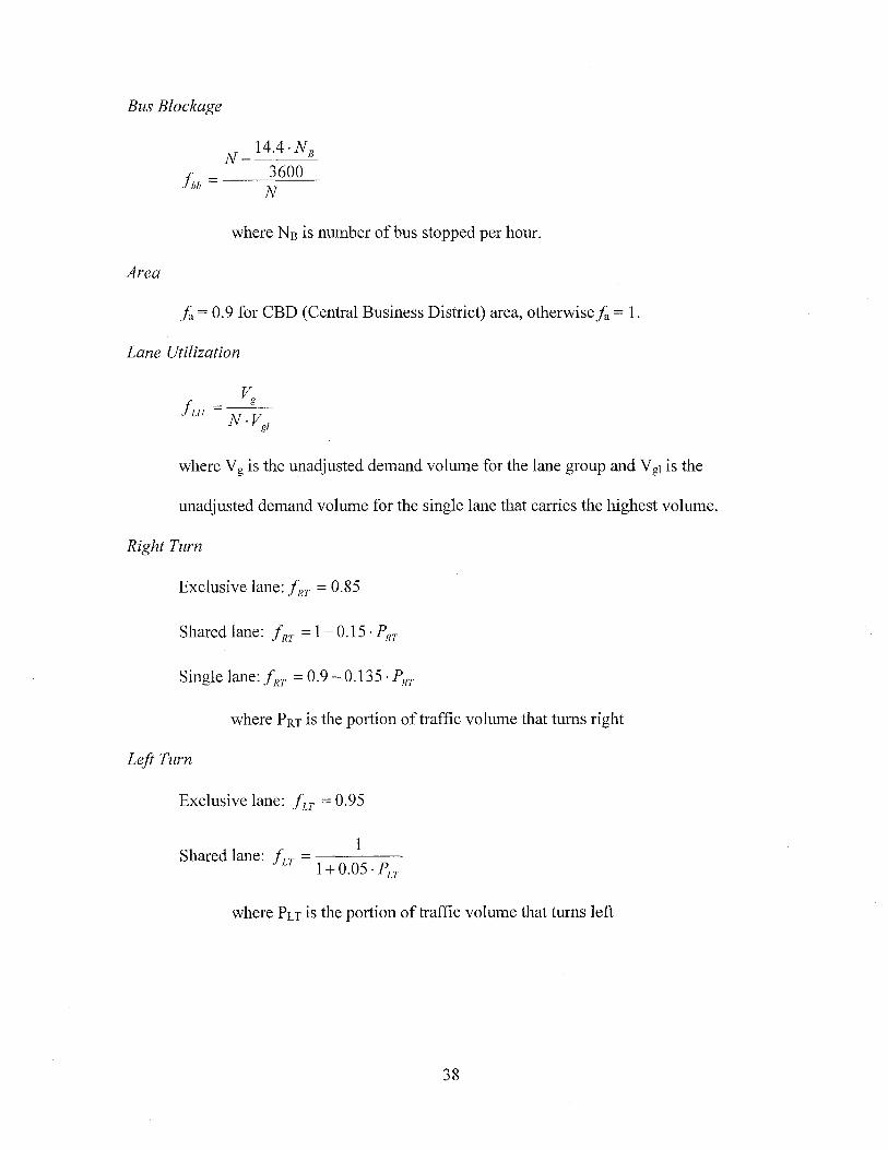
Bus Blockage
N_ 14.4.N/3r _ 3600
Jbb - N
where NB is number of bus stopped per hour.
Area
fa = 0.9 for CBD (Central Business District) area, otherwisefa = 1.
Lane Utilization
Vg
fLU = N.Vgl
where Vg is the unadjusted demand volume for the lane group and Vgl is the
unadjusted demand volume for the single lane that carries the highest volume.
Right Turn
Exclusive lane: fliT = 0.85
Shared lane: fm' =1- 0.15· Pill'
Single lane: f RT = 0.9 - 0.135· PRT
where PRT is the portion of traffic volume that turns right
Left Turn
Exclusive lane: fa = 0.95
1Shared lane: fa =----
1+ 0.05· PLT
where PLT is the portion of traffic volume that turns left
38

Pedestrian and Bicycle
fll1'b =1.0 - PIlI' (1- A1'bT )(1- P IITA )
flpb =1.0 - Pu (1- ApbT )(1- PLTA )
where PRTA (PLTA) = proportion of right (left) turns under protected green
0.6· V1'edApbT =1.0 - ifthe number of turning lanes is the same as the2000
receiving lanes
VA =1.0 -~ if the number of turning lanes is smaller than the number of
phI' 2000
receiving lanes
where Vped is the pedestrian volume
After the calculations for saturation flow rate are completed, delay can be determined
with the following equations:
Capacity
gic· =s··-
I 1 C
where s is saturation, g is green, and C is cycle length.
Peak Hour Factor
PHF = peak - hour· volume4(peak ·15 - min· volume)
Degree ofSaturation
x=Vc
39

Progression Factor
PF = (1- P)/PAg
1-~
C
where
P = proportion of vehicles arriving during green
lPA = supplemental adjustment factor; it is equal to 1 for random arrivals, consult
the HeM for the appropriate value for other conditions.
Delay
Uniform delay
Incremental delay
Initial queue delay
C.(l_K)2d
J=0.5 . --=-C__
1-K. min {X,l.O}C
d2 =900.T.[(X -1)+ (x-l)2 + 8kIX]cT
where k = 0.5, I = 1
d_ 1800· Q" .(l + u) . t cT
3 - T with u =1--(I-min{X,1.0})c· Q
"for t 2 T , else u =0
Once delay is found, LOS can be determined with the criteria in Table 4. Level of
Service A to D indicates traffic performance at the signalized intersection is acceptable,
while E and F indicate unacceptable traffic performance. The criteria are applicable to lane
group, approach, and intersection overall.
40

Delay (sec/veh) Level of Service
s 10 A> 10 but S 20 B
> 20 but S 35 C
> 35 but S 55 D
> 55 but S 80 E
> 80 F
Table 4: Level of Service Table
5.3 Sample Calculation of the LOS that Accounts for Effects of Rainfall
This section uses the intersection ofDole Street and University Avenue to
demonstrate a sample calculation for LOS that accounts for the effects of rainfall. Certain
assumptions about the effects of rainfall on traffic performance are defined. Three scenarios
of wet conditions are created to demonstrate the degree of influence of each factor that
rainfall may have on signalized intersection traffic performance.
As stated in Chapter 3, three traffic performance factors are likely to be affected by
rainfall: Headway (h), Effective Green (gejJ), and Progression Factor (PF). Under wet/light
rain conditions, headway increases by ex%, effective greens decreases by p seconds, and
progression factor worsens by y%.
Currently, little is known about parameters ex, p, and y. Based on the limited studies
by Prevedouros et al. [15], headway is found to be roughly 5% longer under wet/light rain
conditions than in dry conditions.
The saturation flow is defined as s = 3600 , where h is headway in seconds and s ish
saturation flow in vphgpl. Therefore, there is a direct link between hand s. Since 1900 is
commonly used for base saturation flow (so) as recommended in the HCM 2000, base
41

headway (ho) can be calculated to be 1.89. 1fh is 5% longer under wet/light rain conditions,
than hwet = 1.05h = 1.9845 seconds and Swet = 1814 which is 5% less than So =1900. Thus, a
5% increase in headway can be translated into 5% decrease in saturation flow.
Based on the summary from the literature review and information in the FHWA
Weather Management web site, a 2 second decrease in effective green (~ = 2) is used. Li and
Prevedouros [17] observed that start-up lost time is 0.5 seconds shorter for protected left tum
movements, so ~ is 1.5 for protected left turns and 2.0 for all other movements.
Because research on the effects of rainfall on signalized intersection traffic
performance is new, no progression factor research is available yet. Progression Factor is
assumed to increase by 10%, meaning uniform delay (d1) is worsened by 10% due to the
disruption of signal coordination. Thus, a = 5%, ~ = 1.5 and 2 seconds, and y = 10% are used
in the case study herein.
Combinations of the factors are used to create three scenarios of wet conditions to
demonstrate the effects of rainfall on signalized intersection traffic performance with
different degrees of influence.
Wet Scenario 1 considers only the change in saturation headway. Normal saturation
headway is 1.9 seconds. With 5% increase, headway = 2.0 seconds is used. That is
incorporated into the calculation by adjusting the base saturation flow to 1800 from 1900
vehicle per hour green per lane (vphgpl).
Wet Scenario 2 incorporates the change in saturation headway and effective green.
Green times are reduced by 1.5 seconds for exclusive left-tum movement and 2.0 seconds for
all other movements during the computation.
42

Wet Scenario 3 incorporates the changes in saturation headway, effective green, and
progression factor. PF = 1.1 under wet/light rain condition instead of PF = 1.0 for dry
conditions is incorporated into the computation to account for longer start-up lost time and
lesser utilization of the clearance (Y+AR) interval on through movement lane groups.
Microsoft Excel formatted tables are presented below, Table 5 - 8, to illustrate the
calculation process of LOS under Wet Scenario 3 at the Dole Street and University Avenue
intersection. The columns highlighted in gray are displaying the changes in the Wet Scenario
3 from the normal conditions.
FIELD DATA
15-min volumesApproach Movement 01 02 03 04 %HV Width % Slope Park Bus/hr Peds. % turn V
~ TH 140 158 159 201 5.2 12 0 658
~ LT 7 13 14 22 10.7 12 100 563 NB RT 81 68 96 117 1.1 12 3 N N 40 100 362
~ TH+RT 154 148 182 158 3.9 12 3.6 6425 5B LT 41 44 51 52 7.4 12 -3 N N 22 100 188
~ TH+LT 73 55 64 77 1.5 12 93 2697 WB TH+RT 46 52 46 49 2.1 12 0 N N 29 86 1938 EB TH+RT+L 58 42 42 41 3.3 12 0 N N 55 4 183
~LT,RT
Table 5: Field Data
SATURATION FLOWS AND FLOW RATIOS
RT)
(dry. h-1.9, 50-1900)(wet: h=2.0, 50=1800)
Assume L = 4 sec/phase, Y+AR = 5 sec
Approach Movement N w a HV q P bb LU RT LT pb 5
e----1- TH 2 1 1 0.95 0.99 1 1 1 1 1 1 1 3372
~ LT 1 1 1 0.90 0.99 1 1 1 1 0.950 1 1 15213 NB RT 2 1 1 0.99 0.99 1 1 1 0.850 1 1.000 1 2981
--t- TH+RT 3 1 1 0.96 1.02 1 1 1 0.995 1 1.000 1 52465 5B LT 1 1 1 0.93 1.02 1 1 1 1 0.950 1 1 1615
------L TH+LT 1 1 1 0.99 1.00 1 1 1 1 0.956 1 1 16958 WB TH+RT 1 1 1 0.98 1.00 1 1 1 0.871 1 0.993 1 15249 EB TH+RT+LT 1 1 1 0.97 1.00 1 1 1 0816 0.998 0.983 1 1396
- -Approach Movement ApbT PRTAILTA
TH N NLT N 1
NB RT 0.988 1TH+RT 0.993 0
5B LT N 1TH+LT N 1
WB TH+RT 0.991 0+ + 0 (
Table 6: Saturation Flows and Flow Ratios
43
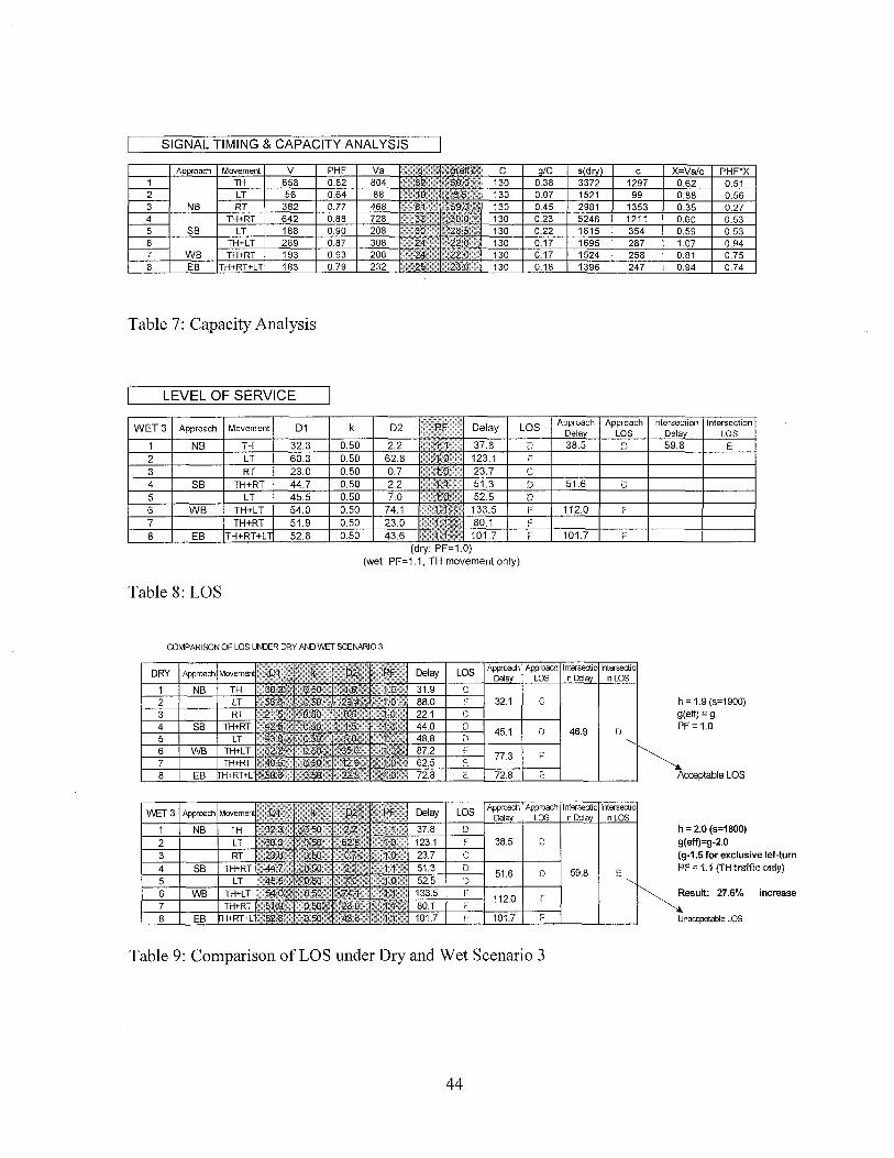
SIGNAL TIMING & CAPACITY ANALYSIS
A roach Movement V PHF Va c X=Va/c PHF*X1 TH 658 0.82 804 1297 0.62 0.512 LT 56 0.64 88 99 0.88 0.563 NB RT 362 0.77 468 1353 0.35 0.274 TH+RT 642 0.88 728 1211 0.60 0.535 SB LT 188 0.90 208 354 0.59 0.536 TH+LT 269 0.87 308 287 1.07 0.947 WB TH+RT 193 0.93 208 258 0.81 0.758 EB TH+RT+LT 183 0.79 232 247 0.94 0.74
Table 7: Capacity Analysis
LEVEL OF SERVICE
WET3 Approach Movement D1 k D2 Delay LOS
1 NB TH 32.3 0.50 2.2 37.8 D2 LT 60.3 0.50 62.8 123.1 F3 RT 23.0 0.50 0.7 23.7 C4 SB TH+RT 44.7 0.50 2.2 51.3 D5 LT 45.5 0.50 7.0 52.5 D6 WB TH+LT 54.0 0.50 74.1 133.5 F7 TH+RT 51.9 0.50 23.0 80.1 F8 EB TH+RT+LT 52.8 0.50 43.6 101.7 F
(dry: PF=1.0)(wet: PF=1.1, TH movement only)
Table 8: LOS
Approach Approach Intersection IntersectionDela LOS Dela LOS38.5 D 59.8 E
51.6 r'.0
112.0 l'
101.7 l'
COMPARISON OF LOS UNDER DRY AND WET SCENARIO 3
DRY Delay LOS
1 NB 31.9 C2 88.0 F 32.1 C h = 1.9 (s=1900)3 22.1 C g(eff) =g4 SB 44.0 D
45.1 D 46.9 DPF=1.0
5 48.8 D6 WB 87.2 F
77.3 E7 62.5 E8 EB 72.8 E 72.8 E Acceptable LOS
WET 3 Delay LOSApproach Approach Intersectio intersectio
Dela LOS nDela nLOS1 NB 37.8 D h = 2.0 (s=1800)
2 123.1 F 38.5 D g(eff)=g-2.0
3 23.7 C (g-1.5 tor exclusive let-turn
4 SB 51.3 D51.6 r' 59.8 E
PF = 1.1 (TH traffic oniy)
5 52.5 DJ
6 WB 133.5 F112.0 F
Result: 27.6% increase7 80.1 F8 EB 101.7 F 101.7 F Unaccpetable LOS
Table 9: Comparison of LOS under Dry and Wet Scenario 3
44

From Table 9, we can see wet conditions lower LOS of some lane groups and
approaches by one grade. The overall intersection LOS is lowered to E and average delay is
extended by 12.9 seconds or 27.6%. Under wet conditions, two out of four approaches
receive LOS = F and average delays approach two minutes.
5.4 Analysis Results of Five Signalized Intersections in Honolulu under
Dry and Wet Conditions
This section presents and discusses the LOS analysis results of five signalized
intersections in Honolulu under dry and wet conditions. The results are presented in four
vertical sections in Table 10. One assuming dry conditions and three with the scenarios of
potential wet weather related impacts. The scenarios, as stated in the previous section,
include reduced saturation flow (wet scenario 1), reduced saturation flow and reduced
effective green (wet scenario 2) and reduced saturation flow, reduced effective green and
worsened progression (wet scenario 3).
The impacts of weather in delay and LOS are shown to be significant. For example,
overall intersection delays increase from dry conditions to wet conditions (scenario 3) by
28%,45%,67%,50% and 37% for Intersections 1 through 5, respectively (Table 10). Under
wet conditions, the LOS worsens by one grade for four out of the five intersections.
Delays tend to be larger for movements served by shorter phases, because of the dis
proportionally larger reduction of the effective green (e.g., protected left tum movements).
Overall, the largest impact is due to the reduction of the effective green and the smallest
impact is due to the progression factor.
45

In order to demonstrate the difference between the normal (dry) LOS and the
prevailing LOS, 21 % is used for the probability of wet conditions in the morning peak (6-8
AM) in the area of the intersections. Accordingly, LOS under normal (dry) condition, wet
scenario 3, and associated probabilities can be used to better portray the true intersection
traffic performance experienced by the motorists. LOS under the worst wet condition (wet
scenario 3) lowers LOS by one grade at four out of the five intersections examined. The
delays under the worst wet condition increase from 28% to 67%. They are shown in the left
half of the Table 11.
The overall prevailing delay at these intersections can also be derived using a
weighted average to combine the delays under both dry and wet. In this way, the prevailing
intersection delays can be calculated as shown in Table 11. Prevailing delays are 6% to 14%
higher than those occurring under dry conditions are.
Although the prevailing LOS did not worsen for any of the five intersections
examined, all of them would be one level worse if volumes were higher by 5% to 10% (e.g.,
intersection 3 is only 0.9 seconds from becoming one level worse.)
Accounting for wet conditions in the capacity analysis of signalized intersections also
reveals operational deficiencies of lanes, lane groups or approaches leading to appropriate
measures, such as modifications to signal timings and reevaluation of the channelization
layout.
46

DRY WET (scenario 1) WET (scenario 2) WET (scenario 3)
h-1.9 (so-1900) h-2.0 (so-1800) h-2.0 (so=1800) h=2.0 (so-1800)
gerrg gerr=ggeff=g-2.0 (g-1.5 for geff=g-2.0 (g-1.5 for
exclusive LT) exclusive LT)PF=1.0 PF=1.0 PF=1.0 PF=1.1 (TH only)
I Approach ILane Group I DelaY LOS Delay LOS Delav LOS Delay LOS
EB TH+RT+LT 72.8 E 79.8 E 96.4 E 101.7 F
WBTH+LT 87.2 F 99.9 F 128.1 F 133.5 F....TH+RT 62.5 E 66.0 74.9t: E E 80.1 F
0 TH 31.9 C 32.7 C 34.6 C 37.8 D:;::(,) NB LT 88.0 F 94.2 F 123.1 F 123.1 F(l)
~ RT 21.1 C 22.4 C 23.7 C 23.7 C(l)- TH+RT 440 D 44.7 D 46.9 D 51.3 D.5 SBLT 48.8 D 50.1
~52.5 D 52.5 E
. Intersection.......~ D 49.6 56.6 ~ E
WB LT+TH 21.7 C 22.2 C 24.3 C 26.5 CN NB
LT 79.7 E 93.5 F 147.3 F 147.3 F...- TH 14.0 B 145 B 16.1 B 17.6 Bt:- ==2! TG 30.6 C 33.3 D 42.7 D 45.5 D
I ·26.4 L.l.£.£...:..: - ~~ . ~EB
LT+TH 51.3 D 58.4 E 89.3 F 92.6 FM RT 12.2 B 14.1 B 16.8 B 16.8 B...- WB LT+TH 85.7 F 102.9 F 171.0 F 174.4 Ft:-~
LT+T= 21.6 C 23.0 C 26.2 C 28.3 C29.9
..(,; ....J.Q1. D
WB LT+TH 22.0 C 22.6 C 24.8 C 27.0 C
"<t NBLT 79.7 E 93.5 F 147.3 F 147.3 F
...- TH 14.3 B 14.8 B 16.5 B 17.9 B
.5 SB TH+= 31.8 C 35.3 D 47.9 D 50.8 D"a. 29.3 .'
EB LT+RT 21.6 C 21.8 C 23,5 C 23.5 CII) NB
LT 71.5 E 83,5 F 127.3 F 127.3 F...- TH 12.8 B 13,5 B 15.1 B 16.4 Bt:- SB TH+RT 21.1 C 21.5 C 23.4 C 25.6 C
- .. ... "":';'
Table 10: Analysis of Five Intersections under Dry and Wet Conditions
DRY (p=0.79) WET (p=0.21) Change in PREVAILING Change inIntersection Delay LOS Delay LOS Delay Delay LOS Delay
I II III IV I v. III V VI I v. V1 46.9 D 59.8 E 28% 49.6 D 5.8%2 26.4 C 38.4 D 45% 28.9 C 9.5%3 29.9 C 50.0 D 67% 34.1 C 14.1%4 26.9 C 40.3 D 50% 29.7 C 10,5%5 24.6 C 33.8 C 37% 26.5 C 7.9%
Table 11: Estimation of Prevailing Delays under Dry and Wet Conditions
47

CHAPTER 6 - SUMMARY AND CONCLUSIONS
6.1 Summary
The study introduced rainfall information estimation with readily available rainfall
data and GIS for transportation applications. The value of the concept was demonstrated with
the application on signalized intersection LOS that accounts for the effects of rainfall.
Three intersection traffic performance parameters that are likely to be affected by
rainfall were considered. The parameters are Saturation Headway (h), Effective Green (getI),
and Progression Factor (PF). Headway increase = 5%, effective green decrease = 2 and 1.5
seconds, and progression factor increase = 10% were used in this study.
Procedure for the estimation of rainfall probability for LOS of signalized intersection
that accounts for the effects of rainfall was established. Rainfall information only during the
peak hours of traffic was used, because roadways reach capacity during these periods and
rainfall has the most significant impact on intersection operation and performance. Besides,
the HCM 2000 requires peak hour of traffic analysis, so it is reasonable to find rainfall
probability only during peak hours of traffic.
Modification to the current HCM procedure for signalized intersection capacity
analysis that accounts for the effects of rainfall was developed in this study. In the proposed
modified procedure, intersection delays and LOS calculation would be executed twice: once
with normal procedure and a second time with the three traffic performance parameters that
are affected by rainfall considered. Rainfall probability at the intersection of interest was
estimated with GIS and readily available rainfall data.
48
A case study on five signalized intersections was calculated to demonstrate the
application of the signalized intersection LOS that accounts for the effects of rainfall. By
using known and assumed rainfall effect parameters, delay under the worst wet condition
(wet scenario 3) increased by 28% to 67%. LOS worsened by one grade at four out of the
five intersections examined. By using 21 % as probability of wet condition, on the average,
the prevailing LOS did not change grade for any of the five intersections but delays were 6%
to 14% higher than these of the dry conditions were. If the traffic volumes were higher by 5%
to 10%, the LOS would have worsened by one letter grade.
6.2 Conclusions
The following key conclusions can be drawn from this study:
• The estimation of rainfall probability for transportation applications is feasible
given that adequate rainfall data are available by NOAA on the Internet for most
metropolitan areas in the U.S. For use in traffic engineering operational studies,
rainfall data intervals of I5-min or I-hour are necessary for the derivation of
rainfall information during peak hours of traffic, with preference given to I5-min
interval data.
• The estimated rainfall probability in the case study gave is based on the frequency
of wet conditions at the location of interest. This probability can applied to the
HCM analysis procedure for the analysis of signalized intersections (and other
procedures in HCM and other engineering fields) to estimate LOS that accounts
for the effects of rainfall. It is an essential part of the concept.
49

• Based on the established and assumed changes in rainfall performance parameters
are correct, the case study showed that four out of the five intersections examined
is performing at a LOS of one grade worse under rainy conditions compared to
dry conditions. It also showed that the delay experienced by motorists at the
intersections examined is 28% to 67% higher under rainy conditions compared
with normal conditions. Development of special signal timing plans for rainy
conditions may be appropriate at the four intersections that their LOS worsened
by one grade.
6.3 Future Research
From the process and results of the study, certain questions were raised. It is
recommended that they be further investigated in the future. The issues include:
• The development of a comprehensive list of the effects of rainfall on the
design and operation of transportation infrastructure.
• Choice and averaging schemes for developing long-term representative
averages of rainfall accumulation and probability by time of day for popular
counties or metropolitan areas in the U.S.
• Specific to signalized intersection, investigation on the effects of rainfall on
capacity analysis parameters.
• Threshold for the amount of rainfall that starts affecting traffic performance at
signalized intersection.
50

APPENDIX A - NOAA HYDRONET
National Weather Service, NOAA, Honolulu Hydronet Archived Data web sitehttp://www.prh.noaa.gov/hnl/hydro/hydronet/hydronet-data.php
Home Page> Hydrolol,lY > Hydronet archived data
H dronet archived dataGeneral Information:The hydronet system began collecting 15-minute rainfall data in July 1994. Currentlythe data is collected from 70 gages located throughout the Hawaiian islands. The datais stored by month, in comma delimited text files so that they can be easily importedinto a spreadsheet Data is available in both Hawaii Standard Time (HS1) as well as inCoordinated Universal Time (UTC). The dataset is updated monthly. The data has notbeen quality controlled, and therefore is not certified by the National WeatherSeNice. Please see the disclaimer for further details.Hydlonet location maps:
Kauai I Oahu I Molokai/lanai I Maui I Hawaii
HST Data UTe Data
2004 2004January February March January February March
April May June April May June
July July
2003 2003January February March January February March
April May June April May June
July August September July August September
October November December October November December
2002 2002January February March January February March
April May June April May June
July August September July August September
October November December October November December
2001 2001January February March January February March
Aoril Mav June Aoril Mav June
51

APPENDIX B - MANUAL FOR GENERATING RAINFALL
PROBABILITY CONTOUR MAPS WITH MAPTITUDE
(1) Maptitude is opened by double clicking the Maptitude icon on the desktop or clicking
once in the menu. If this is the first time that the data are inputted, a new file is created.
Otherwise, an existing file is opened. The "Open a New File" function in the "File" option on
the menu bar is clicked to create a new file. The "Map" option is chosen for the file type on
the pop-up window that shows up immediately after the "Open a New File" function is
clicked. It is illustrated in Figure 6. After the file type is chosen, a new window pops up. The
window is called "Create a Map Wizard." The "General Purpose Map" and "A US City"
New rol" xeru..NJIlOIhI:..---~---
~ ~.,~_ ('" MJll"""-'~('"~.~Ik ('"
AnN~~ .. IhIMc>('" aUSAdl!t ('" A~"r. AOS~ ('" Aee.m
AZlPCode r r",.E.....j,lS
Li1
Figure 6: New File Type window Figure 7: Create a Map Wizard window
options are selected for "Create a New Map" and "Area to Display in the Map", respectively.
Since the study focus is on the City and County ofHonolulu, "Honolulu" is entered for the
city name to retrieve the appropriate map. These steps are illustrated in Figure 7.
52

(2) After the Honolulu map comes up, the map is zoomed in to check ifdetailed streets
are displayed, as illustrated in Figure 8. If the street details do not display, the "US Street
2000" CD that comes within Maptitude package needs to be inserted into the CD-ROM drive
Figure 8: Oahu Base Map withoutDetailed Roadway Information
Figure 9: Open File Window: Input SourceFile for Detailed Roadway Layer
to retrieve street detail information. It is necessary to create a new layer in order to add
detailed roadway information. The layer window is opened by clicking on the "Layer" button
on the function-button menu on top of the screen, right below the menu bar. Once the layer
window is opened, the "Add Layer" function button can be clicked. A window appears and
asks the source for the desired layer information (shown in Figure 9). The geographic file
"ccStreet" on the "US Street 2000" CD is selected as directed by the program on-screen
instruction. Figure 10 illustrates the City and County ofHonolulu base map with added
roadway information.
53

dole and univ case study
Qpenl~l
rain/all report flow chart
lIII sta checklist'lI sta coordinations
Fen- IP_RAlN_SmOOIl2
~ of lJIpe IExcel WOIksheet r. xis)
Figure 10: Oahu Base Map withDetailed Roadway Infonnation
Figure 11: Open File Window: Input SourceFile for Rainfall Probability Infonnation Layer
(3) With the detailed street infonnation in place, the next step adds rainfall probability
infonnation onto the file. To do this, the Excel fonnat infonnation needs to be converted into
appropriate Maptitude fonnat. The rainfall infonnation file is opened with Excel (.xls)
chosen as the file type for the file to be opened. The file used for demonstration here is
named "P_RAIN_SUM_2002," as in Figure 11. After "Open" is clicked, a pop-up window
asks which worksheet to be selected, morning or evening. For the purpose ofdemonstration,
the "morning" worksheet is selected. By clicking "OK.," the "Save Excel Sheet As" window
appears. The file is then saved as "P_rain morning.dbf," as illustrated in Figure 12. After
"Save" is clicked, a pop-up window appears and asks whether to generate a geographic file.
"Yes" is chosen, and the geographic file is saved as "P_rain morning," as illustrated in Figure
13.
54

I-
p_,... evriog JulY c:anlour
.p-'''I''-...a.p_,.. """""",JulY_
Flell'!""8 Ip-,aln~
n..ap IGooqrIllllCFleI·<Ildj
...JllmJU'1
.:.J2D02M..~2lXI2M4II'
2002NoY'-.-12lX12 Del
2002S""
Figure 12: Save File Window: SaveMorning Rainfall ProbabilityInfonnation
Figure 13: Save File Window: Save GeneratedGeographic File into Maptitude ReadableDatabase Fonnat
Immediately following that, a data table and a map window with data points appear.
The data table is the converted Excel file, and the map window with data points is the
geographic file (shown in Figure 14). Before closing both windows, the data are browsed and
the map is checked to see if they appear to be correct. Both windows are then closed because
they are not useful without the base map. The active window is switched back to the
Honolulu map window for further manipulations.
(4) With the "Layers" window open, "Add Layer" is clicked (shown in Figure 15). The
geographic file "P_rain morning," which is created in the previous step, is selected (shown in
Figure 16).
55

'.
ayera
r -
~
l.llblllt.h I Au!ateaIe. I Rename.. I Metadata JecljJ.~ C:~\ccwaIe!aledCOF
I.
I,
p_,011"""""ll-M> .........P-'OII"'-;.P'OII_JuiJ>_
mJ...mM_mM"l'2002N....2002 Oat2lll2S<1>
Flooct... IG~Fio~at:cbll ::Jr 0D0m ..~ ~ ClpotI",,__......
Figure 15: Layer Window (upper right)
Figure 16: Open File Window: Input MorningRainfall Probability Geographic File (right)
Figure 14: Rainfall Probability Geographic Data,both Table and Graph (upper)
(5) While "PJain morning" is selected as the active layer, the "Toolbox" function in the
"Surface Analysis" sub-option under the "Tools" option is clicked. After the "Surface
Analysis" window opens, "All Features" is chosen for "Based on" and "Jul" for "Field"
under the "Settings" tab. July information is chosen here for demonstration purposes. It could
be any month available as desired. "Miles" is selected here for "Display Units." The
desirable unit would be the percentage sign (%) because that is the apt unit for the probability
ofrainfall, but Maptitude does not provide this option. The window is illustrated in Figure
17.
56

5U1face Analysis (Layer: p_'ain morn... EJ
Setti'lgs IOptions
Based on JAil Features
Field
OK
uriace Analysis (Layer: Honolulu_... £J
Selli'lgs Optiom 1Smoothing Level
rv" Outine
OK
Figure 17: Surface Analysis Window,Settings Tab
Figure 18: Surface Analysis Window,Options Tab
(6) The "Options" tab is clicked to further adjust output. On the "Options" tab,
"Smoothing Level" is set to "3" and the "Outline" box is checked, as in Figure 18. Once
"OK" is clicked, the surface analysis window disappears and the data outline is generated on
the Honolulu base map."
C( ~ s-s-...sEnd I~lt <3101 ::£I r-:J
10l10IQ.2JlOO •~
~~lIllll~t03ll~••••l3ll00~~OO t~p~1~OO~~OO R_l.1~OOtolillOO
• SQOOto70.00.70.oorolnOO
l-.IT~
ClNleLiPf
(" Clll'tOUllhi
r. Call1lu Ate. NIh tcb Theme
~I~ ~~~~~("~
r.WInUaI
S8\tWlllt1
Figure 19: Contour Layer Window Figure 20: Manual Theme Window
57

(7) After the outline is generated, the "Surface Analysis" toolbox appears at the upper left
comer of the screen. The "Generate Contour" button is clicked, and the "Contour Layer"
window appears. On the "Contour Layer" window, "Contour Areas with Color Theme" is
selected for "Create Layer", "Manual" is selected for "Contour Interval", and "5" is entered
for "Interva1." An illustration of the window is shown in Figure 19.
(8) The "Save As" window appears after "OK" is clicked on the "Contour Layers"
window. The layer is saved as "P_rain morning July contour." Once it is saved, the "Save
As" window disappears and a color contour layer is overlaid onto the Honolulu base map.
The default color theme of the contour layer does not give clear distinction between classes,
nor intuitive connections between the contour and rainfall information for viewers. The color
theme of the contour layer can be altered as follows. With "Contour Areas" set as the active
layer, the "Color Theme" in the "Map" option on the menu bar is selected. Figure 20 is an
illustration ofthe window. After the "Manual Theme" window appears, the "Style" tab is
selected. Under the "Style" tab, the "Next" or "Previous" buttons are clicked to browse
through the color themes available. The blue theme with white color for the lowest value
range and dark blue color for the highest value range is chosen. Colors within the blue theme
shows the difference between classes clearly and it is assumed that the blue theme provide an
intuitive connection to rainfall information.
(9) With "P_rain morning July contour" selected as the active layer, the first button of
"Surface Analysis" toolbar is clicked. The "Surface Analysis" toolbar appears on the screen
58

after the contour is generated. The first button on the "Surface Analysis" toolbar is
"Calculate Spot Data" (shown in Figure 21). With the "Calculate Spot Data" activated, the
mouse is moved to the desired intersection location on the map to receive the estimated value
of the probability of rainfall. The estimated value appears on the "Surface Analysis" toolbar,
below the function buttons (shown in Figure 22). Figure 22 shows that the estimated rainfall
probability for the sample is 12%. The sample intersection location is the intersection of
Wilder Avenue and Punahou Street.
Figure 21: Surface Analysis Toolbox with"Calculate Spot Data" Button Label
T....,..-..uso.t,..lQ"l 1I \
qw !Estimated Value: \ i"rP12% chance of rainfall \ ,pJ'
1> 'iI ~
""11 III \
~ (f#-et90- ~
\ '"1-'0<.0\< u;.~~ ! ~'1,,~ 1'1 "', \~1~Cld"~~ !f ~~ .r~
S}-~ q..4 ~
'!1~
Location of Interest:Punahou Street and WilderAvenue Intersection
~l j.3
<- i: '" s s~lic!:~ .. <IMsr- 0/' ~%;. <.\<14
S:........... '" !! r'r ~ ...
M.ll' l.lyels__ .. Census Place (2000)
\lltater Area
C State (High)~, Popul ated PI ace
streets
.. p_rain morning Layer
COlltoUl Area Theme0.00 to 5.005.00 to 10.0010.001015.00
.15.001020,00
4t; • 20,001026.00
</' ~'t StleetTYI,et .~ = Highway== Highway (Divided)
= Primary
- Secondary
Local
Vehi 01 e Trail
othero .1 .2 .3
Miles
Figure 22: Sample of Estimation ofRainfall Probability with Maptitude, Punahou Street andWilder Street Intersection, City and County of Honolulu, Oahu, HI, Morning Peak TrafficHours, July 2002
59

APPENDIX C - SUMMARY OF 2002 OAHU PEAK TRAFFIC HOURS RAINFALL PROBABILITY
Rainfall Probability Summary - Morning Peak Traffic Hours
Sta. # Station Name Latitude Longitude Elevation Jan Feb Mar Apr May Jun Jul Aug Sep Oct
1 HonoluluAP2 Wheeler 21.4833 -158.05 820
3 Punaluu Pump 21.5844 -157.8915 20 26 14 24 15 13 16 20 26 29 6
4 Waialua 21.5744 -158.1206 32 6 10 6 0 3 6 10 6 3 0
5 Lualualei 21.4214 -158.1353 113 3 4 6 10 13 0 10 10 0 0
6 Niu Valley 21.3 -157.7333 140 19 21 13 10 6 7 19 10 7 10
7 Poamoho 21.55 -158.1 680 10 8 16 7 3 3 10 10 10 0
8 Waipio 21.4197 -158.0058 410 10 7 3 7 10 7 6 10 " 6.)
9 Kahuku 21.6949 -157.9803 15 13 6 13 16 6 16 6 6 6 10
10 Hakipuu Mauka 21.5036 -157.8575 130 6 21 13 0 6 7 20 26 27 19
11 Palisades 21.4333 -157.95 860 10 21 13 13 13 28 23 23 17 19
12 Kunia substation 21.4 -158.0333 320 6 4 3 3 6 7 3 6 3 10
13 Waimanalo 21.3356 -157.7114 120 29 11 13 20 7 3 16 13 13 19
14 Mililani 21.4667 -158 760 13 10 26 17 23 16 7 13
15 Luluku 21.3875 -157.8094 280 29 8 13 14 17 23 42 32 13 23
16 Ahuimanu Loop 21.432 -157.8373 240 10 14 13 13 14 13 23 35 13 19
17 Waianae 21.4569 -158.1803 40 3 4 0 3 3 0 0 6 0 0
18 Manoa Lyon 21.3333 -157.8 500 42 32 17 17 27 37 52 48 17 23
19 Moanalua 21.3739 -157.8797 230 23 18 10 7 19 20 19 29 7 10
20 Nuuanu 21.3492 -157.8222 780 29 19 21 24 13 53 42 17 29
21 Hawaii Kai GC 21.2992 -157.6647 21 13 7 10 7 23 7 13 26 20 3
22 Maunawili 21.3519 -157.7661 395 43 29 8 33 16 20 58 32 20 19
23 St. Stephens 21.3664 -157.7781 448 19 13 16 17 32 19 7 6
24 Olomana 21.3781 -157.7508 20 16 36 13 14 13 24 "" 19 20 13.).)
25 Palolo FS 21.2994 -157.7944 380 23 18 13 7 6 7 13 13 17 1026 Aloha Tower 21.3039 -157.8625 50 19 0 0 0 7 0 6 10 3 327 Wilson Tunnel 21.3772 -157.8164 1050 32 14 19 20 26 27 42 35 23 2928 Kamehame 21.3039 -157.6814 817 19 4 6 7 6 7 6 6 8 729 WaiawaCF 21.45 -157.9667 770 13 25 10 10 23 31 32 26 17 23
30 WaiheePump 21.4461 -157.8581 196 29 13 27 19 20 42 53 17 23
60

Rainfall Probability Summary - Evening Peak Traffic Hours
Sta. # Station Name Latitude Longitude Elevation Jan Feb Mar Apr May Jun Jul Aug Sep Oct1 HonoluluAP2 Wheeler 21.4833 -158.05 820
3 Punaluu Pump 21.5844 -157.8915 20 26 25 29 26 13 12 17 19 4 194 Waialua 21.5744 -158.1206 32 16 6 6 10 6 3 3 10 6 105 Lualualei 21.4214 -158.1353 113 13 4 3 7 0 0 3 3 3 06 Niu Valley 21.3 -157.7333 140 19 11 10 3 10 3 10 3 3 07 Poamoho 21.55 -158.1 680 23 4 10 10 6 3 3 3 3 108 Waipio 21.4197 -158.0058 410 19 4 13 7 6 3 3 0 0 39 Kahuku 21.6949 -157.9803 15 16 13 3 10 10 16 10 10 6 1910 Hakipuu Mauka 21.5036 -157.8575 130 19 11 13 4 13 17 13 13 10 1011 Palisades 21.4333 -157.95 860 23 18 10 7 10 24 16 6 13 612 Kunia substation 21.4 -158.0333 320 13 4 6 7 0 0 0 3 0 013 Waimanalo 21.3356 -157.7114 120 26 18 19 10 33 33 19 23 10 2614 Mililani 21.4667 -158 760 13 7 10 7 10 3 7 1015 Luluku 21.3875 -157.8094 280 23 8 19 17 17 13 6 10 10 1616 Ahuimanu Loop 21.432 -157.8373 240 23 14 19 13 14 10 3 13 3 1317 Waianae 21.4569 -158.1803 40 16 4 3 7 10 0 3 0 7 318 Manoa Lyon 21.3333 -157.8 500 32 14 20 30 17 33 23 23 17 1619 Moanalua 21.3739 -157.8797 230 16 11 0 7 10 13 6 3 3 1620 Nuuanu 21.3492 -157.8222 780 18 13 25 20 13 27 26 33 2621 Hawaii Kai GC 21.2992 -157.6647 21 16 18 3 23 39 31 19 13 30 2322 Maunawili 21.3519 -157.7661 395 29 17 28 58 29 33 32 42 53 4223 St. Stephens 21.3664 -157.7781 448 16 13 16 20 0 IO 7 1624 Olomana 21.3781 -157.7508 20 26 4 23 14 26 14 20 10 27 325 Palolo FS 21.2994 -157.7944 380 23 11 0 7 3 13 3 3 7 626 Aloha Tower 21.3039 -157.8625 50 10 4 6 10 0 3 3 0 0 327 Wilson Tunnel 21.3772 -157.8164 1050 29 7 19 20 19 27 10 13 13 1328 Kamehame 21.3039 -157.6814 817
.,7 10 3 13 3 3 6 8 3.J
29 WaiawaCF 21.45 -157.9667 770 26 25 16 10 16 17 19 13 20 1330 WaiheePump 21.4461 -157.8581 196 14 19 23 32 13 32 21 30 35
61

APPENDIX D - SAMPLE RAINFALL DATA FILE
Wet Days 1-Apt 2-Apr 30Apr 4-Apr S·Apr 6-Apr 7-Apr 8-Apr 9·Apr 10,Apr 11-Apr 12-Apr 13-Apr 14-Apr 1S-Apr 16-Apr0:15 55.05 55.06 55.07 55.08 55.48 55.48 55.48 55.5 55.5 55,5 55,5 55.5 55,53 55.54 55.56 55.560:30 55.05 55.06 55.07 55.08 55.48 55.48 55.48 55.5 55.5 55.5 55.5 55.5 55.53 55.54 55.56 55.560:45 55,OS 55.06 55.Q7 55.08 55.48 55,48 55.48 55.5 55.5 55.5 55.5 55.5 55.53 55.54 SS.56 55.561:00 55.05 55.06 55.07 55.08 55.48 55.48 55.48 55.5 55.5 55.5 55.5 55.5 55.53 55.54 55.56 55.561:15 55.05 55.06 55.07 55.08 55.48 55.48 55.48 55.5 55.5 55.5 55,5 55.5 55.53 55.54 SS.56 55.561:30 55.05 55.06 55.07 55.08 51i48 55.48 55,48 55.5 555 55.5 55.5 55.5 55.53 55.54 55.56 55.561:45 55.05 55.06 55.Q7 55.08 55.48 55.48 55.48 55.5 55.5 55.5 55,5 55.5 55.53 55.54 55.56 55.562:00 55.05 55.06 55.07 55.08 55.48 55.48 55.48 55.5 55.5 55.5 55.5 55.5 55.53 55.54 55.56 55.562:15 55,05 55,06 55.07 55.08 55.48 55.48 55.48 55.5 55.5 55.5 55.5 55,5 55.53 55.54 55.56 55.562:30 55.05 55.06 55.07 55.08 55.48 55.48 55.48 55.5 55.5 55.5 55,5 55.5 55,53 55.54 55.56 55.562:45 55.05 55.06 55.07 55.08 55.48 55.48 55.48 55.5 55,5 SS.5 55.5 55.5 55.53 55.54 55.56 55.563:00 55.05 55.06 55.07 55.09 55.48 55.48 55.48 55.5 55.5 55.5 55,5 55.5 55.53 55.54 55.56 55.563;15 55.05 55.06 55.07 55.09 55.48 55.48 55.48 55.5 55.5 55.5 55.5 55.5 55.53 55,54 55,56 55.563:30 55.05 55.06 55.07 55.1 55.48 55.48 55.48 55.5 55.5 55.5 55.5 55.5 55.53 55.54 55.56 55.563:45 55.05 55.06 55.07 55.1 55.48 55.48 55.48 55.5 55.5 55.5 55.5 55.5 55.53 55.54 55.56 55.564:00 55.05 55.06 55.07 55.1 55.48 55.48 55.48 55.5 55.5 55.5 55.5 55.5 55.53 55.64 55,56 55.564:15 55.05 55.06 55.07 55.1 55.48 55.48 55.48 55.5 55.5 55.5 55,5 55.5 55.53 55.54 55.56 55.564;30 55.05 55.06 55.07 55.11 55.48 SS.48 55.48 55.5 55.5 55.5 55.5 55.5 55.53 55.54 SS.56 55.564:45 55.05 55.06 55.08 55.11 55.48 55.48 55.48 55.5 55.5 55.5 55.5 55.5 55.54 55.54 55.56 55.565:00 55.05 55.06 55.08 55.11 55.48 55.48 55.48 55.5 55.5 55.5 55.5 55.5 55.54 55.54 55.56 55.565:15 55.05 55.06 55.0B 55.12 55.48 55.48 55.48 55.5 55.5 555 55.5 55.5 5554 5554 55.56 55.565:30 55.05 55.06 55.08 55.14 55.48 55.48 55.48 55.5 55.5 55.5 55.5 55.5 55.54 55.54 55.56 55565:45 55.05 55.06 55.08 55.15 55.48 55.48 55.48 55.5 55.5 55.5 55.5 55.5 55.54 55,54 55.56 55,566:00 55.05 55.06 55.08 55.17 55.48 55.48 55.48 55.5 55.5 SS5 55.5 55.5 55.54 55.54 55.56 55.566:15 55.05 55.06 55.08 55,18 55.48 55.48 55.48 55.5 55.5 55.5 SS.5 55.5 55.54 55.54 55.56 55.566:30 55.05 55.06 55.08 55.18 55.48 55.48 55.48 55.5 55.5 55.5 55.5 55.5 55.54 55.54 55.56 55.566:45 55.05 55.06 55.08 55.18 55.48 55.48 55.48 55.5 55.5 55.5 55.5 55.5 55,54 55,54 55.56 55.567:00 55.05 55.06 55.08 55.19 55.48 55.48 55.48 55.5 55,S 55.5 55.5 55.5 55.54 55.54 55.56 55,567:15 55.05 55.06 55.08 55.19 55.48 55.48 55.48 55.5 55.5 55.5 55.5 55.5 55.54 55.54 5556 55,567:30 55.05 55.06 55.08 55.19 55.48 55.48 55.48 55.5 55.5 55.5 55.5 55.5 55.54 55,54 55.56 55,567:45 55.05 55.06 55,08 55.19 55.48 55.48 55.48 55.5 55.5 55.5 55.5 555 55.54 55.54 55.56 55.568:00 8 55.05 55.06 55,08 55.19 55.48 55.48 55.48 55.5 55.5 55.5 55,5 55.5 55.54 55.54 5556 55.568:15 55,05 55.06 55.08 55.19 55.48 55.48 55.48 55,5 55.5 55,5 55.5 55.5 55.54 55,54 55.56 55.568:30 55.05 55.06 55.08 55.19 55,48 SS48 55.48 55.5 SS.5 55,5 55.5 SS.5 55.54 55.54 55,56 55.568:45 55.05 55.06 55,08 55.19 55.48 55.48 55.48 55.5 55.5 55.5 55.5 55.5 55.54 55.54 55.56 55.569;00 55,05 55.06 55.08 55,19 55.48 55.48 55.48 55,5 55.5 55.5 55.5 55.5 55.54 5555 55,56 55.569:15 55.05 55.06 55.08 55.19 55.48 55.48 55.48 55.5 55.5 55.5 55.5 55.5 55.54 55.55 55.56 55.569:30 55.05 55.06 55.08 55.19 55.48 55.48 55.48 55.5 55.5 55.5 55.5 55,5 55.54 55.55 SS56 55.569:45 55.05 55,06 55.08 55.19 55.48 55.48 55.48 55.5 55.5 55.5 55.5 55.5 55.54 55.55 55.56 55.56
10:00 55.05 55.06 55,08 55.19 55.48 55.48 55.49 55.5 55.5 55.5 55.5 55.5 55.54 55.55 55.56 55.5610:15 55.05 55.06 55.08 55.19 55.48 55.48 55.49 55.5 55.5 55.5 55.5 55.5 55.54 55.55 55.56 55.5610:30 55,05 55.06 55.08 55.19 55.48 55.48 55.49 55.5 SS.5 55.5 55.5 55,5 55.54 55.SS 55.56 55.5610;45 55.05 55.08 55.08 55.19 55.48 55.48 55.49 55.5 55.5 55,5 55.5 555 55.54 55.55 55.56 55.5611:00 55.05 55.06 55.08 55.19 55.48 55.48 55.49 55.5 55.5 55.5 SS.5 55.5 55.54 55.55 55.56 55.5611:15 55.05 55.06 55,08 55,19 55.48 55.48 55.49 SS.5 55.5 55.5 55.5 55.5 55.54 55.56 55.56 55.5611:30 55.05 55.06 55,08 55.19 55.48 55.48 55.49 55.5 55.5 SS.5 55.5 55.5 55.54 55.55 55.56 55.5511:45 55,05 55.06 55.08 55.19 55.48 55.48 55.49 55.5 55.5 55.5 55.5 55.5 55.54 55.55 SS.56 55.5612.:00 55.05 55,06 5508 55.19 55.48 55.48 55.49 55.5 55.5 55.5 55.5 55.5 65.54 55.55 55.56 55.5612:15 55.05 55.06 55,08 55.19 55.48 55.48 55.49 55.5 55.5 55.5 55.5 55.5 55.54 55.55 55.56 55.5612:30 55.05 55.06 55.08 65.19 55.48 55.48 55.49 55.5 55.5 55.5 55.5 55.5 55.54 55.55 55.56 55.5612:45 55.05 55,06 55.08 55.19 55.48 55.48 55.49 55.5 55.5 55.5 55.5 55.5 .55.54 55.56 55.56 55.5613:00 55.05 55.06 55.08 55.19 55.48 55.48 55.49 55.5 55.5 55.5 55.5 55.5 55.54 55.56 55.56 55.5613:15 55.05 55.06 55.08 55.19 55.48 55.48 55.49 55.5 55.5 55.5 55.5 55.5 55.54 55.56 5556 55.5613:30 55.05 55.06 55.08 55.19 55.48 55.48 55.49 55.5 55,5 55.5 55.5 55.5 55.54 55.56 55.56 55.5613:45 55.05 55.06 55.08 55.19 55.48 55.48 55.49 55.5 55.5 55.5 55.5 55.5 55.54 55.56 55,56 55.5614:00 55.05 55,06 55.08 55.19 55.48 55.48 55.49 55.5 55.5 55.5 55.5 55,5 55.54 55.56 55.56 55.5614:15 55.05 55.06 55.08 55.19 55.48 55.48 55.49 55.5 55.5 55.5 55.5 55.5 55.54 55.56 55.56 55.5614:30 55.05 55.06 55.08 55,19 55.48 55.48 55.49 55.5 55.5 55.5 55.5 55.5 55.54 55.56 55.56 55.5614:45 55.05 55.06 55.08 55.19 55.48 55.48 55.49 55.5 55,5 55.5 55.5 55.5 55.54 55,56 55.56 55,5615:00 55.06 55.06 55.08 55.19 55.48 55.48 55.49 55.5 55.5 55.5 55.5 55.5 55.54 55.56 55.56 55.5615:15 55.06 55.06 55.08 55.19 55.48 55.48 55.49 55,5 55.5 55.5 55.5 55,5 55.54 55.56 55.56 55.5615:30 55,06 55.06 55,08 55.19 55.48 55.48 55.49 55.5 55.5 55.5 55.5 55.5 55.54 55.56 55.56 55.5615:45 55.06 55.W 55.08 55.19 55.48 55.48 55.49 55.5 55.5 55.5 55.5 55,5 55.54 55.56 55.56 55.5616:00 55.06 55.06 55,08 55.19 55.48 55.48 55.49 55.5 55.5 55.5 55.5 55.5 55.54 55.56 55.56 55.5616:15 55,06 55.06 55.08 55.19 55.48 55.48 55.49 55.5 55.5 55.5 55.5 55.5 55.54 55.56 55.56 55.5616:30 55.06 55.06 55.08 55.19 55.48 55.48 55.49 55.5 55.5 55.5 55.6 55.5 55.54 55.56 55.56 55.5616:45 55.06 55.06 55.08 55.19 55.48 55.48 55.49 55.5 55.5 SS.5 55.5 55.5 55.54 55.56 55.56 55.5617:00 7 55.06 55W 55.08 55.19 55.48 55.48 55.49 SS.5 55.5 55.5 55.5 55.5 55.54 55.56 55.56 55.5617:15 55.06 55.06 55,08 55.2 55.48 55,48 55.49 55.5 55,5 55.5 55.5 55,5 55.54 55.56 55.56 55.5617:30 55.06 55.06 55.08 55.21 55.48 55.48 55.49 55.5 55.5 55.5 55.5 55.5 55.54 55.56 55.56 55,5617:45 55.06 55.06 55.08 55.22 55.48 55.48 55.49 SS.5 55.5 55.5 55.5 55.5 55.54 55.56 55.56 5$.5618:00 55,06 55.06 55.08 55.23 55.48 55.48 55.49 55.5 SS.5 55.5 55.5 55.5 55.54 55.56 55.56 55.5618:15 55.06 55.06 55.08 55.23 55.48 55.48 55.49 55.5 55.5 55.5 55.5 55,5 55.54 55.56 55.56 55.5618:30 55.06 55.06 55.08 55.24 55.48 55.48 55.49 55.5 55.5 55.5 SS.5 55.5 55,54 55.66 55.56 55.5618;-45 55,06 55.06 55.08 55.31 55.48 55.48 55.49 55.5 55.5 55.5 55,5 55.5 55.54 55.56 55.56 55.5619:00 55.06 55.06 55.08 55,37 55.48 55.48 55.5 55'.5 55.5 55.5 55.5 55.5 55.54 55.56 55.56 55,5619:15 55.06 55.06 55.08 SS.4 55.48 55.48 SS5 55.5 55.5 55,5 55.5 55.5 55.54 55.56 55.56 55.5619:30 55.06 55.06 55,08 55.43 55.48 55.48 55.5 55.5 55.5 55.5 55.5 55.5 55.54 55.56 55.56 55.5619:45 55.06 55.06 55.08 55.43 55.48 55.48 55.5 55.5 55.5 55.5 55.5 55.5 55.54 55.56 55.56 55.5620:00 55.06 55.06 55,08 55.43 55.48 55.48 55.5 55,5 55.5 55.5 55.5 55.5 55.54 55.56 55.56 55.5620:1$ 55.06 55.06 55.08 55.43 55.48 55.48 55.5 55.5 55.5 55.5 55.5 55.5 55.54 55.56 55.56 55,5620:30 55.06 55.06 55.08 55.43 55.48 55.48 55.5 55,5 55,5 55.5 55.5 55.5 55.54 55.56 55.56 55.5620:45 55.0£ 55.06 55.08 55.44 55.48 55.48 55.5 55.5 555 55.5 55.5 55.5 55.54 55.56 55.56 55.5621:00 55.06 55.06 55.08 55.44 55.48 55.48 55.5 55.5 55.5 55.5 55.5 55.5 55.54 55.56 55.56 55.5621:15 55.06 55.06 55.08 55.45 55.48 55.48 55.5 55,5 55,5 55.5 55,5 55.5 55.54 55.56 55.56 55.5621:30 55.06 55.06 55.08 55.45 55.48 55.48 55.5 55.5 55,5 55,5 55.5 55.5 55.54 55.56 55.56 55.5621:45 55.06 55.0£ 55.08 55.46 55.48 55.48 55,5 55.5 55.5 55.5 55.5 55,5 55.54 55.56 55.56 55.5622:00 55.06 55.06 55.08 55.47 55.48 55,48 55.5 55.5 55.5 55.5 55.5 55.5 55.54 55.56 55.56 55.5622:15 55.06 55.06 55,08 55.47 55.48 55.48 55.5 55.5 55.5 55.5 55.5 55,5 55.54 55.56 55.56 55.5622.;30 55,06 55.06 55.08 55.47 55.48 55.48 55.5 55.5 55.5 55.5 55.5 55.5 55.54 55.56 55.56 55.5622:45 55,06 55.06 55,08 55.47 55.48 55.48 55.5 55.5 55.5 55.5 55.5 55.5 55.54 55.56 55.56 55.5623:00 55.06 55.06 55.08 55.47 55.48 55.48 55.5 55.5 55.5 55.5 55.5 55.5 55.54 55.56 SS.56 55.5623:15 55,06 55.06 55,08 55.47 55.48 55.48 55.5 55.5 55.5 55.5 55.5 55.5 55.54 55.56 55.56 55.5623:30 55.06 55.06 55.08 55.47 55.48 55.48 55.5 55.5 55.5 55.5 55.5 55.5 55.54 55.56 55.56 55.5623:45 55.06 55.06 55.08 55.48 55.48 55.48 55.5 55.5 55,5 55.5 55.5 55.53 5554 55.56 55.56 55.560:00 55.06 55.06 55.08 55.48 55.48 55.48 55.5 55.5 55.5 55.5 55.5 55,53 55.54 55.56 55.56 55.56
morning rainevening rain
WaiheePump 10 11 12 13 14 15 18
days observ. Interval mlnlhour30 96 15 60 72' hours
day!;; day!;; in April 2002each column:: 1 day
# Of morning #ofeverrlllll8 7
pofmornlngraln pofevenlng rain27% 23%
62

REFERENCES
1. OECD Road Research Group. Adverse Weather, Reduced Visibility and Road Safety
- A Road Research Report. Organisation for Economic Co-operation and
Development (OECD), Paris, France, 1976.
2. OECD Scientific Expert Group. Road Surface Characteristics: Their Interaction and
Their Optimization - A Road Transportation Research Report. Organisation for
Economic Co-operation and Development (OECD), Paris, France, 1984.
3. Pisano, P., and L. C. Goodwin. Surface Transportation Weather Applications.
http://209.68.41.108/itslib/AB02H261.pdf. Accessed in June 2003.
4. Middleton, W.E.K. Vision through the Atmosphere. University of Toronto Press,
1952.
5. Olivera, F., and D. Maidment. Geographic Information System Use for Hydrologic
Data Development for Design of Highway Drainage Facilities. Transportation
Research Record 1625, Transportation Research Board, National Research Council,
Washington, D.C., 1998, pp. 131-138.
6. Highway Capacity Manual 2000, Transportation Research Board, National Research
Council, Washington, D.C., 2000.
7. Martin, P. T., H. J. Perrin, and B.G. Hansen. Modifying Signal Timing during
Inclement Weather. Transportation Research Record 1748, Transportation Research
Board, National Research Council, Washington, D.C., 2001, pp. 66-71.
63

8. Agbolosu-Amison, S. J. and A. W. Sadek. Inclement Weather and Traffic Flow at
Signalized Intersections: A Case Study from Northern New England. Transportation
Research Board, 83rd Annual Meeting CD, Washington, D.C., 2004.
9. Kockelman, K. M. Changes in the Flow-Density Relation due to Environmental,
Vehicle, and Driver Characteristics. In Transportation Research Record 1644, TRB,
National Research Council, Washington, D.C., 1998, pp. 47-56.
10. Holdener, D. J. M. The Effect of Rainfall on Freeway Speeds. In Institute of
Transportation Engineers Journal, Volume 68, Issue 11, Washington D.C., November
1998.
11. Federal Highway Administration. Road Weather Management. U.S. DOT, 2003.
http://www.ops.fhwa.dot.gov/Weather.
12. Lamm, R., E. M. Choueiri, and T. Mailaender. Comparison of Operating Speeds on
Dry and Wet Pavements of Two-Lane Rural Highways. In Transportation Research
Record 1280, TRB, National Research Council, Washington D.C., 1990, pp. 199-207.
13. Ibrahin, A. T., and F. L. Hall. Effects of Adverse Weather Conditions on Speed-Flow
Occupancy Relationships. In TranspOliation Research Record 1457, TRB, National
Research Council, Washington D.C., 1994, pp. 184-191.
14. Kyte, M., Z. Khatib, P. Shannon, and F. Kitchener. Effect of Environmental Factors
on Free-Flow-Speed. Transportation Research Record 1776, Transportation Research
Board, National Research Council, Washington, D.C., 2001, pp 60-68.
15. Prevedouros, P. Potential Effects ofWet Conditions on Signalized Intersection LOS.
Unpublished Paper, University of Hawaii at Manoa, 2003.
64

16. National Weather Service Forecast Office. Hydronet Achieved Data, NOAA, 2003.
http://www.prh.noaa.govlhnl/hydro/hydronet/hydronet-data.php. Accessed in June
2003.
17. Li, H. and P. D. Prevedouros. Detailed Observation of Saturation Headways and
Start-up Lost Times, Transportation Research Record 1802, Transportation Research
Board, National Research Council, Washington, D.C., 2002, pp. 44-53.
65