rain, emotions and voting for the status quoftp.iza.org/dp10350.pdf · november 2016 abstract rain,...

Forschungsinstitut zur Zukunft der ArbeitInstitute for the Study of Labor

DI

SC

US

SI

ON

P

AP

ER

S

ER

IE

S

Rain, Emotions and Voting for the Status Quo

IZA DP No. 10350

November 2016

Armando N. MeierLukas SchmidAlois Stutzer

Rain, Emotions and Voting for the Status Quo

Armando N. Meier University of Basel

Lukas Schmid University of Lucerne

Alois Stutzer University of Basel

and IZA

Discussion Paper No. 10350 November 2016

IZA

P.O. Box 7240 53072 Bonn

Germany

Phone: +49-228-3894-0 Fax: +49-228-3894-180

E-mail: [email protected]

Any opinions expressed here are those of the author(s) and not those of IZA. Research published in this series may include views on policy, but the institute itself takes no institutional policy positions. The IZA research network is committed to the IZA Guiding Principles of Research Integrity. The Institute for the Study of Labor (IZA) in Bonn is a local and virtual international research center and a place of communication between science, politics and business. IZA is an independent nonprofit organization supported by Deutsche Post Foundation. The center is associated with the University of Bonn and offers a stimulating research environment through its international network, workshops and conferences, data service, project support, research visits and doctoral program. IZA engages in (i) original and internationally competitive research in all fields of labor economics, (ii) development of policy concepts, and (iii) dissemination of research results and concepts to the interested public. IZA Discussion Papers often represent preliminary work and are circulated to encourage discussion. Citation of such a paper should account for its provisional character. A revised version may be available directly from the author.

IZA Discussion Paper No. 10350 November 2016

ABSTRACT

Rain, Emotions and Voting for the Status Quo*

Do emotions affect the decision between change and the status quo? We exploit exogenous variation in emotions caused by rain and analyze data on more than 400 ballot propositions in Switzerland for the years 1958 to 2014 to address this question. The empirical tests are based on administrative ballot outcomes and individual postvote survey data. We find that rain decreases the share of votes for a change. Our robustness checks suggest that changes in the composition of the electorate or changes in information acquisition do not drive this result. In addition, we provide evidence that rain might have altered the outcome of several high-stake votes. We discuss the psychological mechanism and document that rain reduces the willingness to take risks, a pattern that is consistent with the observed reduction in the support of change. JEL Classification: D03, D72 Keywords: emotions, voting, status quo, risk aversion, rain, direct democracy, turnout Corresponding author: Alois Stutzer Faculty of Business and Economics University of Basel Peter Merian-Weg 6 4002 Basel Switzerland E-mail: [email protected]

* We thank Toke Aidt, Sandro Ambuehl, Douglas Bernheim, Monika Bütler, Allison Carnegie, Marco Casari, Robert Erikson, Olle Folke, Matthias Flückiger, Patricia Funk, Roland Hodler, Katharina Hofer, Jo Thori Lind, Alessandro Lizzeri, Ulrike Malmendier, Ulrich Matter, Stephan Meier, Reto Odermatt, Pietro Ortoleva, Johanna Rickne, Hannes Schwandt, Jan-Egbert Sturm, Michaela Slotwinski, Roberto Weber, Lauren Young and seminar participants at the Universities of Zurich and Basel for helpful comments. We also thank conference participants at the Annual Meeting of the American Political Science Association, the Annual Meeting of the European Public Choice Society, the Annual Meeting of the Swiss Society for Economics and Statistics and the Joint EJPE-IGIER Bocconi-CEPR Conference on Political Economy. Armando Meier acknowledges funding by the Swiss National Science grant #P1BSP1_165329 and thanks Columbia Business School for its hospitality. Lukas Schmid acknowledges funding from the Swiss National Science grants #NPBBEP1_141484 and #100017-141317/1.

mailto:[email protected]

1 Introduction

Politics fuels emotions and emotions motivate political engagement and decisions over and

above cognitive evaluations.1 Emotions can serve as a beneficial guide to decision-making,

but sometimes may lead decision-makers astray.2 We study how emotions affect the funda-

mental decision about whether to keep or change the status quo. We exploit rainfall as an

exogenous source of variation in emotions (Lambert et al., 2002; Hirshleifer and Shumway,

2003; Kamstra, Kramer and Levi, 2003;) and examine whether voters are more or less likely

to support a policy change on a rainy voting weekend.

Most decisions involve the choice between keeping the status quo or opting for change.

The human tendency to maintain the status quo, usually the default option, has been doc-

umented in a variety of real life choices.3 The status quo effect has been attributed to risk

preferences and uncertainty (Samuelson and Zeckhauser, 1988), loss aversion (Kahneman,

Knetsch and Thaler, 1991), and also cognitive load (Danziger, Levav and Avnaim-Pesso,

2011; Augenblick and Nicholson, 2016). Little is known, however, about the effect that emo-

tions have on the tendency to choose the status quo in such decisions. This is surprising in

view of the recent contributions in economics which have demonstrated the pervasive impact

of emotions on human decisions (Loewenstein, 2000; Caplin and Leahy, 2001; Kahneman

and Thaler, 2006; DellaVigna, 2009; Haushofer and Fehr, 2014).

In this paper, we explore the effect of emotions on the support of the status quo. We

analyze a novel data set that contains more than 860,000 municipal-level vote outcomes

from 417 propositions at the federal level of Switzerland’s direct democracy between 1958

and 2014. We use administrative voting and individual postvote survey data to estimate the

effect of rain on the propensity to vote for the status quo. We find that rain on a voting

weekend decreases support for changing the legal status quo. A simple simulation indicates

1For reviews on emotions in economics, politics and political philosophy, see, e.g., Elster (1998, 1999) andMarcus (2000).

2An excellent general account on emotions and decision-making is provided in Lerner et al. (2015). Thebridge to economic reasoning is nicely built in Loewenstein (2000).

3These include, for example, the decision to use default retirement plans (O’Donoghue and Rabin, 2001),the greater willingness to become an organ donor if donating is the status quo option (Johnson and Goldstein,2003), or supporting the incumbent candidate (Lee, 2008).

1

that this rain effect potentially swayed several vote outcomes. We address two explanations,

other than emotional reactions, for a substantial negative relationship between rain and the

share of yes votes. First, we test whether changes in the composition of the constituency

can explain the empirical regularity. Second, we investigate whether the use of different

information channels is responsible for the rain effect. In addition, we show that the effect is

driven by citizens who cast their ballot card on the voting weekend, rather than by those who

vote beforehand by mail. Moreover, our results suggest that the effect of rain also prevails

in narrow and high-turnout votes.

Switzerland provides a unique setting to study citizens’ policy choices as most major

political decisions are determined by popular votes. These political decisions are highly

salient due to broad media coverage. Vote outcomes from referendums and popular initiatives

are binding. Examples of high-stake ballots include Switzerland’s vote on its membership

in the European Economic Area, a proposal to introduce a federal debt brake, and several

votes on the introduction of a comprehensive minimum wage scheme. Importantly, Swiss

voters have substantial experience with popular votes. Thus, our findings are robust to

the concern that the influence of psychological factors vanishes as individual experience

increases (List, 2003; Levitt and List, 2008). Finally, the framing of the decision emphasizes

the potential new future legal situation. In the official description of the ballot proposals,

the new alternative statutory or constitutional law is explicitly discussed in reference to the

current legal status quo. Accordingly, an approval of the policy change always requires a yes

vote, while adherence to the status quo requires a no vote. This enables a straightforward

interpretation of the effect of rain on vote outcomes.

What might drive this rain effect? We discuss several psychological mechanisms and

conclude that a specific version of the projection bias (Loewenstein, O’Donoghue and Rabin,

2003) offers the most plausible explanation. Emotions affect risk aversion and consequently

alter the evaluation of the policy options (Schwarz, 2012). The intuition is straightforward.

While positive emotions lead to more optimistic evaluations of change, negative emotions lead

to more cautious appraisals. Consistent with this, we document that reported willingness to

take risks is lower if it rains, based on complementary data.

2

We think that our results are important for two reasons. First, the direct democratic

votes that we study are collective decisions with major policy implications. If psychological

factors alter such collective choices, we should take this evidence into account for institutional

design. Second, our findings from field data suggest that negative emotions lead people to

favor the status quo. This tendency may be relevant in other domains – for instance, in labor

market decisions and health choices. Choice architects should thus be aware that decisions

may be affected by external emotional cues that systematically affect peoples’ trade-offs

between change and status quo.

This study relates to at least three strands of research. First, we add to a growing

literature that explores the role of emotions for decision-making in field settings (DellaVigna,

2009). Studies have exploited the fact that the performance of a favored sports team affects

mood, and consequently influences the ruling of judges, the evaluation of politicians, and

family conflicts (Healy, Malhotra and Mo, 2010, 2015; Card and Dahl, 2011; Fowler and

Montagnes, 2015; Eren and Mocan, 2016). Our study is, to our knowledge, the first that

explicitly tests whether the effect of emotions operates through “an impact on risk-aversion

... or a projection of the emotions to economic fundamentals” (DellaVigna, 2009, p. 359).

Second, we add to the new field of behavioral political economy that investigates why and

how citizens vote based on a broader account of human motivation. In this vein, DellaVigna

et al. (2016) document that social image concerns are important in explaining why people

vote. Augenblick and Nicholson (2016) show that choice fatigue can cause voters to make

decision shortcuts, for example, by voting for the status quo. Berggren, Jordahl and Pout-

vaara (2010) provide evidence that voters use visual cues, such as a candidate’s physical

appearance, as a heuristic to assess politicians.

Third, we contribute to the recent work on the effects of rain on elections. This literature

has argued that rainfall exclusively alters the cost of voting. This in turn impacts turnout

(Hansford and Gomez, 2010; Fraga and Hersh, 2011; Lind, 2015a; Arnold and Freier, 2015;

Fujiwara, Meng and Vogl, 2016) and participation rates in political rallies (Madestam et al.,

2013). Our findings suggest that rainfall not only alters voting results by changing the

constituency, but also directly affects the voting decisions of citizens. Our evidence from

3

observational data complements previous experimental findings by Bassi (2015) who shows

that weather conditions affect how voters evaluate the incumbent.

We proceed as follows. Section 2 provides background on the institutional environment

in Switzerland, our data sources, and our empirical strategy. Section 3 explores the effect of

rain on vote outcomes. We first present the main results and then conduct two placebo tests.

In addition, we explore alternative explanations for the main empirical regularity including

a change in composition of the electorate due to rain. Finally, we highlight the substantial

size of the rain effect. In Section 4, we discuss aspects of the likely mechanism behind the

relationship between rain and voting behavior and other aspects that are relevant for the

assessment of the generality of our findings. Section 5 concludes and suggests directions for

future research on emotions and choice between change and the status quo.

2 Institutions, Data and Empirical Strategy

2.1 Institutions

A citizen’s ability to decide on basic policy issues is fundamental to any democratic system

with elements of direct democracy. Direct democratic participation is a constitutive element

of the Swiss political system. Citizens decide on several policy propositions throughout the

year. Most important for our study is that a yes vote is always a vote for change. This

means that we can concentrate on the share of yes votes when evaluating the support for

change. The outcome of a popular vote is binding and may lead to major changes in public

policy. Notable important propositions include votes on the participation in the integrated

market of the European Union, fundamental changes to the federal tax code, and votes on

the future of the social security system.4

Ballot propositions can be divided into two categories: referendums and popular initia-

tives. A mandatory referendum takes place for every proposed amendment of the federal

constitution. In addition, federal laws approved by both chambers of parliament are put to

4An overview of popular votes at the federal level in Switzerland is provided on the official webpage ofthe Swiss government at https://www.admin.ch/gov/en/start/documentation/votes.html.

4

https://www.admin.ch/gov/en/start/documentation/votes.html

a popular vote if a committee of citizens submits 50,000 valid signatures. Popular initiatives

allow citizens, parties, and interest groups to propose constitutional amendments. A vote

takes place if the initiators have collected 100,000 valid signatures.

People fill in ballot cards at home and traditionally bring them to the ballot box on the

voting weekend. The ballot card arrives by mail two to three weeks before the vote takes

place. The ballot boxes are open on Saturday and Sunday and they are located in the city

hall or in a public building. The ballot cards state the type of popular vote and the title of

the proposition.

As an alternative to voting at the polling station, all Swiss cantons have gradually in-

troduced postal voting since 1978, most of them during the 1990s (Hodler, Luechinger and

Stutzer, 2015). This has altered the way people vote. While all voters formerly had to cast

their votes at the ballot box before the introduction of postal voting, a fifth of voters did

so in 2005 (Federal Chancellery, 2005). However, roughly one third of the voters still cast

their votes via mail in the week preceding the voting weekend (Federal Chancellery, 2005).

More than half of the votes cast in our sample were cast at the ballot box or within the week

before the vote.

2.2 Data

We make use of three comprehensive data sources for our analysis. First, we draw on admin-

istrative data on municipal vote outcomes for the years 1958–2014 from the Swiss Federal

Statistical Office (SFS, 2015). These data contain vote outcomes (for the averages across mu-

nicipalities, see Figure A.2) and turnout information for all Swiss municipalities and federal

propositions. In total, we have data on more than 860,000 municipal-level vote outcomes

from 417 propositions in 2,538 municipalities. On average, there are three voting week-

ends per year (see Figure A.1 for the distribution over months). We complement this data

with vote recommendations for propositions from parties based on Swissvotes, a database

maintained by the University of Berne and Annee Politique Suisse (Swissvotes 2012).

For additional analyses, we also add information on the electoral strength of parties at

the municipal-level in federal parliamentary elections from 1971–2007. For each voting date,

5

we assign the latest election outcome, or, in the case of the years before 1971, the electoral

outcome in 1971. These data are provided by the Swiss Federal Statistical Office (SFS, 2015).

Second, we base our analysis on individual voting decisions from postvote surveys for the

years 1996–2006 (FORS 2014).5 Several Swiss universities and the private research institute,

GFS, administer these postvote surveys, called VOX surveys, after each voting weekend.

A representative sample of roughly 1,000 voters is contacted by phone. The resulting data

contain information on whether and how respondents voted, the method of voting (via mail or

via ballot box at the polling station), a few socio-economic characteristics, political ideology,

knowledge about the vote issues and which information channels voters used.

Third, we use data on local rainfall that stems from the Swiss Federal Office of Meteo-

rology (MeteoSwiss 2015). It includes information on rainfall between 7 a.m. and 7 p.m.6

An advantage of our setting is the great variation in rainfall over time and space due to the

specific topography of Switzerland shaped by the Jura Mountains and the Alps.7 We gath-

ered rain data on all popular votes from 1958–2014 based on 116 automated meteorological

stations (see Appendix, Figure A.6, for a map of the stations).

To construct a variable for rainfall at the municipal-level, we interpolate station-level

rain data using the inverse distance weighting function for the nearest three stations. As

rain conditions in the mountains can be considerably different from those in the lowlands

and in the foothills of the Alps, we excluded 17 weather stations above an altitude of 2,000

meters. We further dropped all stations with a distance larger than 30 kilometers from a

municipality’s set of stations. We construct an indicator variable for rain that is equal to

one for a municipality if it rained any time between 7 a.m. and 7 p.m. on the Saturday or

the Sunday of the voting weekend.

5Note that for the year 1997 there is no municipality identifier available, thus we cannot use the data forthis year.

6Our rain variable at the 12-hour-level provides us with a more relevant time frame than most studiesthat also include nightly rainfall.

7Appendix Figures A.1, A.3, A.4 and A.5 provide an illustration of the temporal and spatial variation inrainfall in our data. The descriptive statistics are depicted in Table A.1 in the Appendix.

6

2.3 Empirical Strategy

The extensive municipal and individual data allow us to explore the effect of rain, controlling

for a substantial amount of observed and unobserved heterogeneity. We examine the effect

of rain on political decisions with the following econometric model using municipal data:

Yjp = ηj + δp + αRainjp +X ′jpβ + εjp, (1)

where j indexes municipalities, p indexes proposals; Yjp is our outcome of interest, namely

the share of yes votes in percentage points; ηj is a municipality fixed effect; δp is a proposition

fixed effect; α is the coefficient of interest; Rainjp is a dummy that is one if it rained in

municipality j; X ′jp is a matrix of covariates that may include variables such as turnout; β

is a vector of coefficients; and εjp is an idiosyncratic error term.

Standard errors account for clustering in the 26 cantons. We cluster at the cantonal level

to take into account both spatial correlation in rain and serial correlation in voting behavior.

This is analogous to state-level clustering for the United States, which is commonly regarded

as most conservative option and therefore the recommended one (Cameron and Miller, 2015).

Note that the null hypothesis that rain has no effect on the share of yes votes is rejected for

both data sets at conventional significance levels whether we use voting weekend, municipality

or two-way clustered standard errors.

We complement the analysis of municipal voting data with a detailed investigation of

how rain affects voting decisions using individual-level data and building on an estimation

equation similar to equation (1). This allows us to control for covariates as well as to estimate

the effect of rain on ballot box voters and postal voters separately. Appendix B provides a

detailed exposition of the model at the individual-level.

7

3 Rain, and Votes Against the Status Quo

3.1 Main Results

We show the bivariate relationship between the share of yes votes and rain in the raw data in

Figure 1. It displays the density of the share of yes votes in percentage points on dry (dashed

black line) and rainy days (solid blue line). The figure reveals that the share of yes votes

is considerably lower on rainy days. While the average yes share is 47.1 percentage points

on dry days, it is 46.2 percentage points on rainy days. This descriptive evidence should be

interpreted with caution. It might be that municipalities with high average rainfall are more

likely to oppose political reforms per se. We therefore turn to the regression analysis that

allows us to identify the effect of rain on the share of yes votes holding constant characteristics

that are specific to municipalities and propositions. We first consider the administrative,

municipal-level data and second the individual-level postvote survey data.

Figure 1: Rain and the Share of Yes Votes in Percentage Points

0.0

05.0

1.0

15.0

2Ke

rnel

Den

sity

Est

imat

e

0 10 20 30 40 50 60 70 80 90 100Yes Share in Percentage Points

No Rain Rain

Note: The figure shows two estimated densities of the yes vote share in percentage points for rainy votingweekends (blue solid line) and dry voting weekends (black dashed line). The density estimates stem from theEpanechnikov kernel function (bandwith = 3.0) based on 862,670 municipal-level vote outcomes.

Municipal Data — Table 1 presents our main results from the municipal data set.

Column (1) shows the raw difference in means. It indicates that propositions on rainy voting

8

weekends have a yes share that is about one percentage point lower than propositions on

dry voting weekends. This difference might be the consequence of temporal and spatial

dependence that creates a spurious relationship between rain and the share of yes votes.

Table 1: Effect of Rain on the Share of Yes Votes in Percentage Points,Municipal Data 1958–2014

Dependent Variable Share of Yes Votes [0–100]

(1) (2) (3) (4)

Rain Indicator -0.98∗∗ -1.32∗∗ -1.28∗∗∗ -1.24∗∗∗

(0.39) (0.57) (0.38) (0.39)

Proposal FE 3 3 3

Municipality FE 3 3

Mun. Trends 3

Observations 862,670 862,670 862,670 862,670Clusters 26 26 26 26R-squared 0.00 0.69 0.71 0.72

Note: The table shows the estimated effect of rain on the share of yes votes

in percentage points using OLS. Standard errors (in parentheses) are clustered

at the cantonal level. The rain indicator is 1 for all rainy voting weekends.

∗ p < 0.10, ∗∗ p < 0.05, ∗∗∗ p < 0.01

To hold constant common shocks caused by timing, such as seasonal effects or aggregate

opinion shocks, we include proposal fixed effects in column (2). The estimated coefficient

for rain is -1.32. In column (3), we add municipality fixed effects to address the concern

that municipalities with more rain may be more conservative. The effect of rain remains

unchanged. Finally, we include linear municipal time trends in column (4) to demonstrate

that spatio-temporal trends do not drive our results. In Table A.2 in the Appendix, we

provide evidence that the rain effect prevails in specifications with cubic trends, municipal-

month or municipal-year fixed effects. The stability of the coefficient estimate to the inclusion

of these granular fixed effects implies that short-term fluctuations in rain drive our results.

We use specification (4) as our baseline model for the municipal data set throughout the rest

9

of the paper to capture not only time and spatial fixed effects, but also municipality-specific

trends.8

In an additional analysis, we regress the share of yes votes on terciles of rainfall to

investigate the functional form between the two variables. Figure 2 depicts that even very

light, as well as, light levels of rainfall decrease the share of yes votes. These low levels of

rainfall are analogous to dark skies and some rain.9 The results are similar if we use rainfall

quintiles instead of terciles as indicated in Figure A.8 in the Appendix.

Figure 2: Flexible Relationship between Rain in Terciles and the Share of YesVotes in Percentage Points, Municipal Data

-4-3

-2-1

01

Effe

ct o

f Rai

n (in

Per

c. P

oint

s)

Med.-Heavy Rain(4.3-105]

Light Rain(0.8-4.3]

Very Light Rain(0.0-0.8]

Rain in mm

Note: The figure shows coefficient estimates for the effect of rain on the share of yes votes in percentage pointstogether with a 95% confidence interval (thin line) and a 90% confidence interval (thick line) using municipaldata. The point estimates are based on regression model (4) in Table 1 with indicator variables for the tercilesof rainfall. The reference category is zero rainfall.

Postvote Survey Data — We also estimate the effect of rain on the propensity to

vote yes using individual data from postvote surveys. The results are reported in Table 2.

The point estimate of rain is consistently negative in all specifications and varies between

-1.84 and -3.15. It is robust to the inclusion of proposal and municipality fixed effects as

well as covariates that comprise age dummies, gender, dummies for income categories and a

dummy for holding a university degree. We also estimate the relationship between rain and

8The coefficient of rain is statistically significant when we use the voting weekend, the municipality or thetwoway clustered standard errors, see Table A.3 in the Appendix.

9The Swiss Metereological Service classifies rain of 2mm per hour as heavy rain. In comparison, rainfallof up to 4mm over the entire voting weekend can be considered as light rain. Therefore, we name the twolowest terciles light and very light rain.

10

voting yes using a more flexible functional form. Figure A.7 in the Appendix demonstrates

that the negative effect of rain is pronounced even for propositions with light rainfall, which

is qualitatively equivalent to the results from municipal data. In sum, our main estimates

from the two high resolution data sets suggest that there is a sizeable effect of rain on vote

choices. This effect prevails even when we control for a large set of fixed effects and individual

covariates.

Table 2: Effect of Rain on the Share of Yes Votes in Percentage Points,Postvote Survey Data 1996-2006

Dependent Variable Voted Yes [0,100]

(1) (2) (3) (4)

Rain Indicator -2.02∗ -1.84∗ -2.93∗∗ -3.15∗∗

(1.13) (1.05) (1.38) (1.28)

Proposal FE 3 3 3

Municipality FE 3 3

Covariates 3


Note: The table shows the estimated effect of rain on the

propensity to vote yes in percentage points using OLS. Stan-

dard errors (in parentheses) are clustered at the cantonal

level. The rain indicator is 1 for all rainy voting weekends.

∗ p < 0.10, ∗∗ p < 0.05, ∗∗∗ p < 0.01

3.2 Placebo Tests

We examine the plausibility of the rain effect in two ways. First, we conduct a placebo test

by randomizing rainfall across voting weekends. Second, we exploit an institutional change –

the introduction of postal voting – which allows voters to cast their votes before the official

voting weekend.

Random Rainfall — Due to the high spatial and time series correlation in rainfall data,

the precision of the rain effect may be overestimated (Lind, 2015b; Cooperman, 2016). To

11

address this concern, we follow Lind (2015b) and Fujiwara, Meng and Vogl (2016) by using

flexible time trends. In a separate specification, we use municipal-year fixed effects to account

for spatial correlation over time (see Table A.2 in the Appendix). We also check whether the

estimated rain effect is spurious in a placebo study that randomizes voting weekend rainfall

(Lind, 2015b). We assign future or past voting weekend weather randomly to another voting

weekend and run our baseline specification 500 times. Intuitively, this method randomizes

rain maps across voting weekends. We then compare our main results in Table 1 with the

distribution of placebo estimates.

Figure 3: Randomized Rainfall

Treatment t-Value

0.0

5.1

.15

.2.2

5.3

.35

.4D

ensi

ty

-4 -3.5 -3 -2.5 -2 -1.5 -1 -.5 0 .5 1 1.5 2 2.5 3 3.5 4Placebo t-Values

Empirical t-Density Theoretical t-Density

Note: This figure shows the empirical distribution of t-values under placebo rainfall, the average t-value underour baseline specification, as well as the theoretical t-distribution. Since we randomize rain at the voting weekendlevel, we use standard errors clustered at voting weekend in all specifications here. The theoretical t-distributiontherefore has 163 degrees of freedom. Note that we have fewer observations, 671,000 on average, than in ourbaseline sample. This is because our panel is unbalanced and randomization of votedate rainfall therefore leadsto missing values. To obtain a plausible t-value for the comparison, we computed the effect of true votingweekend rainfall in the same reduced samples and averaged the resulting t-values. The average t-value of thetreatment, -2.77, is depicted by the blue line. The critical empirical t-value at the 1% level is -2.72. The t-valueof the treatment in the full sample with voting weekend clustering is -3.20.

Figure 3 shows the resulting coefficients divided by their standard errors (black solid line)

together with the theoretical t-distrbution (black dotted line). As expected in a placebo

study, the distribution of t-values is centered at zero. The vertical blue line depicts the

t-value of our baseline specification. It indicates that the size of the coefficient estimate lies

in the outer tail of the coefficient distribution. The obtained t-value of -2.77 is slighly larger

12

in absolute value than the critical empirical t-value at the 1% level, which is -2.72. Thus,

our regression coefficient for rain is statistically significant at the 1% level when compared

to the empirical distribution of t-values under the null hypothesis.

Postal Voting — Swiss cantons gradually introduced the possibility of postal voting in

addition to voting at the ballot box, which resulted in an increase in individuals who cast

their ballot card by mail before the voting weekend (Hodler, Luechinger and Stutzer, 2015).

We exploit this procedural change to shed light on the plausibility of our findings. Since

rain on the voting weekend should have no effect on early postal voters, we expect larger

effects in time periods with no postal-voting option. Accordingly, we compare the effect size

of rain before and after the introduction of postal-voting based on the municipality data.

For the individual-level data, we test whether postal voters are affected by rain on the voting

weekend. For both samples, we explore whether voters with access to postal voting might

be affected by rain before the voting weekend.

Table 3 reports the results for the municipal data. The effect of rain in periods with no

postal voting option is -1.4 percentage points (columns 1 and 2). It is 0.4 percentage points

higher than the effect on municipalities that offered supplementary postal voting (columns 3

and 4), although the two coefficients are not statistically significantly different. Note that the

negative effect of rain after the introduction of postal voting is plausible as still a considerable

fraction of voters continued to vote at the ballot box.

A substantial fraction of voters, 37% on average in 2005, cast their votes in the week

preceding the voting weekend (Federal Chancellery, 2005). This means a rain effect is plau-

sible in the week before the voting weekends in periods with postal voting, while we expect

to observe no effect of rain preceding the voting weekend in periods without postal voting.

Columns (2) and (4) in Table 3 add an indicator for the share of rainy days in the five days

prior to the voting weekend. This indicator ranges from 0, no rain, to 1, rain on all days.

The entries suggest that the pre-weekend rain has no effect if there is no option to vote by

mail, while pre-weekend rain has an effect if there is this possibility. For instance, if it rains

13

Table 3: Sensitivity of the Rain Effect to Postal Voting


No Postal Postal(1) (2) (3) (4)

Rain Indicator -1.40∗∗∗ -1.39∗∗∗ -1.00∗∗∗ -0.95∗∗

(0.46) (0.48) (0.45) (0.45)

Share of Rainy Days -0.24 -2.18∗∗

Week Before Vote (1.08) (0.9)

Proposal FE 3 3 3 3

Municipality FE 3 3 3 3

Mun. Trends 3 3 3 3


Note: The table shows the estimated effect of rain on the share of yes votes in

percentage points using OLS. Standard errors (in parentheses) are clustered at the

cantonal level. The rain indicator is 1 for all rainy voting weekends. The vari-

able capturing the share of rainy days in the five days before the vote date ranges

from 0 to 1. On average it rained two out of five days before the voting weekend,

which is equivalent to a share of rainy days in the week before the vote of 0.4.

∗ p < 0.10, ∗∗ p < 0.05, ∗∗∗ p < 0.01

one day more than expected given the typical rainfall patterns, the yes share is reduced by

a substantial 0.5 percentage points.

The individual postvote survey data allow us, in addition, to distinguish traditional ballot

box voters from postal voters, as respondents are asked about their methods of voting. In

columns (1) and (2) of Table 4, we estimate separate regressions for the ballot box voters

and postal voters. The effect of rain on the propensity of ballot box voters to vote yes

is -5.95 percentage points and roughly six times larger than the point estimate of rain on

individuals who vote by mail, which is by itself not statistically significantly different from

zero.10 Instead, postal voters might be affected by rain in the last week before the voting

weekend. While our estimates are imprecise, the results from the postvote survey data are

10The share of voters voting at the ballot box as indicated by the postvote survey seems to be reliable.In 2005, slightly more than 20 percent voted at the ballot box according to the postvote survey, which isconsistent with official estimates (Federal Chancellery, 2005). Unfortunately, this was the only year in whichcomprehensive administrative data on postal voting was gathered.

14

Table 4: Effect of Rain on Ballot Box vs. Postal Voters

Dependent variable Voted Yes Ballot Box Voter

(1) (2) (3)Ballot Box Voters Postal Voters All

Rain Indicator -5.95∗∗∗ -1.02 -1.54(1.88) (1.57) (2.62)

Share of Rainy Days -0.62 -6.52 -0.60Week Before Vote (2.62) (4.96) (4.81)

Proposal FE 3 3 3

Municipality FE 3 3 3

Covariates 3 3 3

Observations 11,159 17,903 29,473Clusters 26 26 26R-squared 0.28 0.24 0.35

Note: The table shows the estimated effect of rain on the propensity to vote yes (columns 1 and 2) inpercentage points using OLS. Standard errors (in parentheses) are clustered at the cantonal level. Therain indicator is 1 for all rainy voting weekends. The variable capturing the share of rainy days in the fivedays before the vote date ranges from 0 to 1. On average it rained two out of five days before the votingweekend, which is equivalent to a share of rainy days in the week before the vote of 0.4. The dependentvariable in column (3) is either 0 or 100, depending on whether the voter voted at the ballot box or not.∗ p < 0.10, ∗∗ p < 0.05, ∗∗∗ p < 0.01

consistent with the results from the municipal data. In a further check, we test whether rain

affects the probability to observe ballot box voters rather than postal voters on a rainy voting

weekend in column (3). The results suggest that there is no selection to the ballot box due

to rainfall. In conclusion, the results from the two data sets provide strong evidence that

the effect of rain is not spurious, but is substantially driven by those voters whose decisions

– due to the timing of their vote casting – are expected to be most affected by rainfall.

3.3 Alternative Explanations

We focus on two possible alternative explanations, other than emotions, that could drive the

effect of rain on support for the status quo. First, we explore whether the effect of rain might

operate through a change in the composition of the electorate. Second, we study whether

rain affects individual information acquisition.

Change in the Electoral Composition — A growing literature provides evidence that

rain affects turnout by altering the costs of voting (Hansford and Gomez, 2010; Fraga and

15

Hersh, 2011; Lind, 2015a; Arnold and Freier, 2015; Fujiwara, Meng and Vogl, 2016). If rain

affects the electoral composition by including fewer people who are willing to give up the

status quo, the rain effect could not be interpreted as an emotion effect, but rather as a

compositional effect. We undertake three tests to explore this alternative channel.

First, we examine the relationship between rain and overall turnout. If we regress turnout

on an indicator variable for rain on the voting weekend, municipality fixed effects, proposal

fixed effects and municipal time trends, we estimate a coefficient of the rain indicator of

-0.33 with a standard error of 0.28. We also find no statistically significant effect of rain on

turnout in the postvote survey data, the estimate being +0.59 with a standard error of 1.26.

Several reasons may account for the arguably small and statistically insignificant effect of

rain on turnout. With few exceptions, all municipalities have their own ballot boxes which

translates into short travel distances. This is in contrast to the US context where polling

stations tend to be far away. In addition, polling stations are usually well organized and

queues outside the polling station are very rare.

Figure 4: Flexible Relationship between Rain in Terciles and Turnout in Per-centage Points, Municipal Data

-4-3

-2-1

01

Effe

ct o

f Rai

n (in

Per

c. P

oint

s)


Light Rain(0.8-4.3]


Rain in mm

Note: The figure shows coefficient estimates for the effect of rain on turnout in percentage points togetherwith a 95% confidence interval (thin line) and a 90% confidence interval (thick line) using municipal data. Thepoint estimates come from a regression of turnout on indicator variables for terciles of rainfall while controllingfor municipality fixed effects, proposal fixed effects and municipal time trends. The reference category is zerorainfall.

Previous research has pointed out that the effect of rain on turnout might not be uniform

with heavy rain having the most detrimental effect on voters’ probability of going to the

16

polls. To explore this, we estimate our main equation for turnout by using three dummies

for the different terciles of rainfall. Figure 4 shows the results of this regression. The effect

of rain on turnout is only statistically significantly different from zero for medium to heavy

rainfall.11

In stark contrast, the effect of rain on the share of yes votes is negative and statistically

significant already at very low levels of rainfall. Figure 5 compares the results for both

turnout and the propensity to vote yes (both in percentage points). The figure indicates

that low levels of rainfall do not depress turnout but still decrease the yes share. At least at

low and medium levels of rain, the effect on the yes share seems not to be driven by changes

in aggregate turnout due to rainfall.

Figure 5: Effect of Rain on Turnout vs. Effect of Rain on the Share of Yes Votes,Municipal Data

-2.5

-2-1

.5-1

-.50

.5

Effe

ct o

f Rai

n (in

Per

c. P

oint

s)


Light Rain(0.8-4.3]


Rain in mm

Effect on Turnout Effect on Yes Share

Note: The figure shows coefficient estimates for the effect of rain on turnout in percentage points (black dots)and on the yes share in percentage points (blue triangles) using municipal data. The dots are retrieved fromregression model (4) in Table 1 using turnout or the yes share as dependent variable and with indicator variablesfor terciles of rainfall instead of one indicator. The reference category is zero rainfall.

Even if rain has no effect on aggregate turnout, it might be that rain affects voting

outcomes via the turnout channel if the turnout reaction is heterogeneous across groups

in the population. Consider, for instance, a situation in which leftist voters with a high

propensity to vote yes abstain on rainy days, while rightist voters with a low propensity to

11This effect is driven by the highest quintile of rainfall (see Figures A.9 and A.10 in the Appendix).

17

vote yes are motivated to go to the polls if it rains. If the positive and negative effect are

similar in absolute value terms and both groups are of similar size, aggregate turnout does

not change, but rain affects voting outcomes purely by changing the electoral composition.

In our second test, we explore the possible unequal impact of rain on turnout for different

groups of voters with individual-level data. Tables A.4 to A.6 report the turnout reaction

for different subsamples of voters conditional on past turnout, knowledge, party preferences,

ideology and socio-demographic characteristics. None of the point estimates are statistically

significantly different from zero, but there are some differences in absolute size. Table A.4

indicates that the negative rain effect is more pronounced for voters who rarely vote than for

marginal- and always-voters. Similarly, rain seems to depress the turnout of voters with a low

level of political knowledge more than the turnout of voters with high political knowledge.

Table A.5 divides voters along party lines and reveals that individuals with centrist views are

most likely to abstain on rainy voting weekends. As socio-economic conditions are important

determinants of turnout and voting behavior, we also divide the sample by income, age, and

gender. Table A.6 reveals that high-income individuals and women are most likely to react

to rain.

How do these heterogeneous turnout reactions translate into aggregate voting outcomes?

To explore this question, we simulate the compositional effects of rain based on the hetero-

geneous turnout reactions reported in Tables A.4 through A.6. In a first step, we use the

turnout differences across groups derived from the above variables, weight them according to

group size and multiply them with the average yes share of the particular group. Finally, this

allows us to predict the yes share for each group under rainfall corrected for compositional

changes. We do the same computation for days with no rainfall. The comparison of the

predicted yes shares allows us to obtain an estimate for the change in yes votes as a conse-

quence of compositional changes. We then correct our main estimate for the effect of rain

on the propensity to vote yes for this composition effect and depict the corrected coefficients

in Figure A.11 in the Appendix. The blue line indicates the baseline estimate and the black

dots the corrected coefficients derived from the turnout reaction of different groups of voters

across several variables. The figure suggests that the corrected estimates are very similar to

18

the baseline estimates. Accordingly, compositional changes do not drive our main effect of

rain on the support for change.

The reason why compositional changes have a negligible impact on vote outcomes are

twofold. First, the turnout reactions are relatively small and thus alter the electoral compo-

sition only to a small extent.12 Second, preferences for change are not too different across

groups.13

Our third test incorporates proxies for the electoral composition into our main analysis.

We start by controlling for turnout in our preferred specification using municipal data. The

entries in column (1) of Table 5 suggest that controlling for turnout does not affect the

coefficient of rain. It remains statistically significant with a value of -1.3 percentage points.

The estimated coefficient remains equal if we control for turnout deciles, as indicated in

column (2). To account for differential mobilization of parties as a consequence of rain,

we interact turnout with party shares in the last parliamentary elections, both measured

at the municipal-level. Moreover, we interact party shares and turnout with the federal

party recommendations for the votes. We do this because voters of a certain party may

only be motivated to vote when their party issues a recommendation. The size of this

effect may depend on the importance of the proposition, which is why we interact party

recommendations with turnout. In addition, we control for the lagged yes share, to account

for electoral trends. The results reported in column (3) suggest that a flexible control for

electoral composition does not affect the substantive size of the estimate. We also do not

find a heterogeneous reaction in turnout or yes share conditional on whether the a priori

composition of the municipal electorate is rather right-wing, left-wing or center-oriented, see

Table A.7 in the Appendix.

12Note that male voters gain the most weight in the electorate from 47.2% on days with no rain to 48.8%on rainy days.

13The highest spread in preferences for change is between individuals who prefer the left-wing party (52%yes share) and those who prefer the right-wing party (39% yes share).

19

Table 5: Robustness of the Rain Effect to Compositional Changes

Dependent Variable Share of Yes Votes Voted Yes(Municipal Voting Data) (Individual Voting Data)

(1) (2) (3) (4) (5) (6)

Rain Indicator -1.27∗∗∗ -1.27∗∗∗ -1.10∗∗ -3.18∗∗ -3.02∗∗ -3.03∗∗

(0.38) (0.38) (0.52) (1.32) (1.37) (1.33)

Turnout -0.09∗∗∗ -0.15∗∗∗

(0.01) (0.05)

Turnout Deciles 3

Party Shares Last Election 3

Party S. × Turnout 3

Party S. × Party Recomm. 3

Party Recomm. × Turnout 3

Party S. × Party R. × Turnout 3

Lagged Yes Share 3

Preferred Party 3 3

Ideology 3 3

Average Turnout 3 3 3

Means of Voting 3 3 3

Proposal FE 3 3 3 3 3 3

Municipality FE 3 3 3 3 3 3

Mun. Trends 3 3 3

Covariates 3 3 3

Observations 862,670 862,670 703,173 29,510 29,510 29,510Clusters 26 26 26 26 26 26R-squared 0.72 0.72 0.73 0.22 0.22 0.22

Note: The table shows the estimated effect of rain on the share of yes votes (columns 1 to 3) orthe propensity to vote yes in percentage points (columns 4 to 6) using OLS. Standard errors (in paren-theses) are clustered at the cantonal level. The rain indicator is 1 for all rainy voting weekends. Incases of non-available election data, we replaced the missing values by those of the nearest election year.∗ p < 0.10, ∗∗ p < 0.05, ∗∗∗ p < 0.01

We also re-estimate the main specification using the sample of individual voting data. In

column (4) of Table 5, we control for partisan preferences by including dummies indicating

a voter’s most preferred party. In column (5), we control for ideology captured as dummies

based on a left-right scale ranging from 0 to 10. In column (6), we include partisan preferences

and ideology jointly. In all three specifications, we control for for the average turnout and

the means the citizens used to cast the vote. The effect of rain on the probability of voting

yes remains similar in magnitude and statistically significant. In supplementary tests, we

check whether specific parties or ideologies drive our results. We depict the stability of

20

our estimated coefficient of rain on voting yes to leaving out specific parties or ideological

positions in Figures A.12 and A.13 in the Appendix. The results of the three tests strongly

suggest that the negative relationship between rain and voting for the status quo is not due

to a compositional change of the electorate.

Information Acquisition — Instead of changing the composition of the electorate,

rain might affect voting decisions by altering the type of information sources which citizens

consult. If it rains, voters may spend more time reading the information booklet that comes

with the ballot card or instead they may watch television. Our data provides us with infor-

mation about the type of information voters use to gather knowledge about the propositions.

The information channels include TV, radio, newspapers, and official government leaflets. In

a first step, we control for the type of information voters use. The results in column (1) of

Table A.8 in the Appendix show that the estimated effect size is very similar to the baseline

model with a point estimate of -3.25 percentage points. We also check whether rain has

an impact on proposition knowledge, which in turn might affect the voting decision. We

estimate the effect of rain on the probability that a voter knows the exact title of the propo-

sition for all voters as well as for ballot box voters only. The results suggest that rain has no

statistically significant effect on knowledge about a proposition.

3.4 Relevance of the Rain Effect

The results thus far have established a stable and precisely measured effect of rain on the

share of yes votes. One might, however, argue that the size of the rain effect is too small

to affect aggregate vote outcomes. We therefore simulate the impact of rain for all 417

propositions in our sample. Among these popular votes, 32 exhibit a yes share between

48.8% and 51.2%. We illustrate the results showing the propositions for which rainfall could

have changed voting outcomes in Figure 6. The blue triangle depicts the predicted outcome

if it had rained in all municipalities, the orange circle indicates the predicted outcome if

rain had been completely absent across all municipalities.14 The grey square is the official

vote outcome. Among the ten popular votes which might have turned out differently under

14Note that both outcomes are probable, see Appendix, Figure A.5.

21

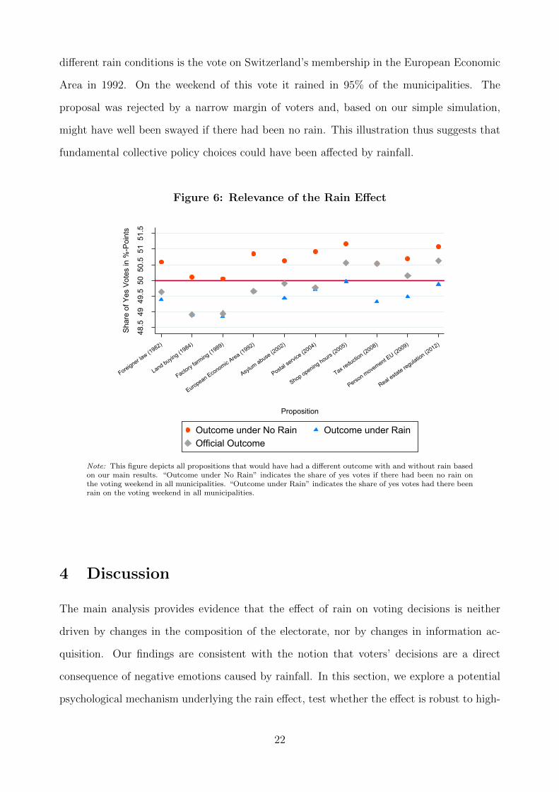
different rain conditions is the vote on Switzerland’s membership in the European Economic

Area in 1992. On the weekend of this vote it rained in 95% of the municipalities. The

proposal was rejected by a narrow margin of voters and, based on our simple simulation,

might have well been swayed if there had been no rain. This illustration thus suggests that

fundamental collective policy choices could have been affected by rainfall.

Figure 6: Relevance of the Rain Effect

48.5

4949

.550

50.5

5151

.5

Shar

e of

Yes

Vot

es in

%-P

oint

s

Foreigner law (1982)

Land buying (1984)

Factory f

arming (1989)

European Economic Area (1992)

Asylum abuse (2002)

Postal se

rvice (2004)

Shop opening hours (2005)

Tax reductio

n (2008)

Person movement E

U (2009)

Real estate regulation (2012)

Proposition

Outcome under No Rain Outcome under RainOfficial Outcome

Note: This figure depicts all propositions that would have had a different outcome with and without rain basedon our main results. “Outcome under No Rain” indicates the share of yes votes if there had been no rain onthe voting weekend in all municipalities. “Outcome under Rain” indicates the share of yes votes had there beenrain on the voting weekend in all municipalities.

4 Discussion

The main analysis provides evidence that the effect of rain on voting decisions is neither

driven by changes in the composition of the electorate, nor by changes in information ac-

quisition. Our findings are consistent with the notion that voters’ decisions are a direct

consequence of negative emotions caused by rainfall. In this section, we explore a potential

psychological mechanism underlying the rain effect, test whether the effect is robust to high-

22

stake situations, examine whether negative emotions may lead specifically to an increase in

support for traditionalist conservative positions, and also whether the effect is driven by

swing voters.

Psychological Mechanisms — Up to this point our results suggest that incidental emo-

tions, defined as emotions caused by factors that should not be relevant for a particular

decision context (Lerner et al., 2015), may have an impact on vote choices. A large body

of literature in behavioral economics, psychology and medicine has demonstrated that bad

weather leads to negative emotions (see, e.g., Lambert et al., 2002; Kamstra, Kramer and

Levi, 2003; Hirshleifer and Shumway, 2003). However, how do these negative emotions af-

fect individual support for the status quo? In our view, the most plausible explanation is a

specific version of state dependent preferences.

The most prominent characterization of state dependent preferences is formalized by the

concept of the projection bias (Loewenstein, O’Donoghue and Rabin, 2003). The main idea

is that individuals project their current preferences, which depend on their emotional state,

into the future. These projected preferences distort the perception of future payoffs. In

particular, the projection bias suggests that transitory emotional states have a large effect

on decision-making. Important forward-looking decisions, even after careful deliberation,

may thus be swayed by contemparenous emotional cues (Loewenstein, 2000). An example

of projection bias is the empirical regularity that a 4WD vehicle looks much more useful

on rainy days, while a convertible car offers a higher projected future utility on sunny days

(Busse et al., 2015).15 In our context, voters who are in a negative emotional state caused

by rainfall may project this negative state into the future when evaluating the payoffs of a

new policy. Note, however, that the theoretical formulation of projection bias does not yield

any prediction with respect to exactly how emotions affect the support for the status quo.

A psychological mechanism that specifies how positive and negative emotions may alter

status quo support is subsumed under feelings-as-information (Johnson and Tversky, 1983;

Schwarz, 2012). It postulates that individuals become more risk averse if they experience

15For further examples see Conlin, O’Donoghue and Vogelsang (2007) and Simonsohn (2010).

23

negative emotions. As a consequence, they may evaluate the status quo relatively more

favorable.16 Evidence from laboratory experiments support the claim that individuals act

more risk averse if they experience negative emotions (Schwarz, 2012; Haushofer and Fehr,

2014; Cohn et al., 2015). Previous contributions that use observational data have pointed

out that feelings-as-information may affect stock market behavior, since positive emotions

caused by good weather increase stock returns (Hirshleifer and Shumway, 2003; Kamstra,

Kramer and Levi, 2003; Bassi, Colacito and Fulghieri, 2013).17

Exploring the psychological mechanism that drives the effect of emotions requires data

on risk aversion. As the postvote survey data offers no information on risk attitudes, we use

data from the Swiss Household Panel. This survey contains information on the willingness

to take risks from a similar population in the same institutional environment. If feelings-

as-information is the reason why emotions affect support for the status quo, we expect that

individuals are less willing to take risks on rainy days.

In Table 6, we show the estimates of the rain effect on a dichotomized measure of will-

ingness to take risks derived from a scale ranging from 0 to 10, whereby 10 indicates “I am

willing to take risks” and 0 indicates “I avoid taking risks”.18 If the willingness to take risks

is larger than the median value 5, the dependent variable is 100, and zero otherwise. We

regress this indicator on a rain indicator that is one if there was any rain on the exact day

of the interview in the respective municipality. We find that rain decreases the probability

of being ready to take risks by roughly 2.7 percentage points in the most comprehensive

specification in column (4). There, we control for month and municipality fixed effects as

well as for several covariates including gender, age dummies, income and education dummies.

Using the same rainfall terciles as with the municipal-level data, we find that light rain most

heavily affects the willingness to take risks as depicted in Figure A.14 in the Appendix. This

16In the present policy context, voters decide on reforms which are inherently risky, see e.g., Fernandezand Rodrik (1991) and Augenblick and Nicholson (2016).

17A competing hypothesis to feelings-as-information is the mood maintenance hypothesis. It postulatesthat individuals become more risk-averse if they experience positive emotions, because they want to preservetheir current positive emotional state, and conversely, they are more-risk affine if they experience negativeemotions (Isen, 2005).

18This questionnaire item is very similar to the one in the German Socio-Economic Panel, which wasexperimentally validated by Dohmen et al. (2011). Note that our results hold also when we use the the scalefrom 0 to 10 rather than an indicator variable.

24

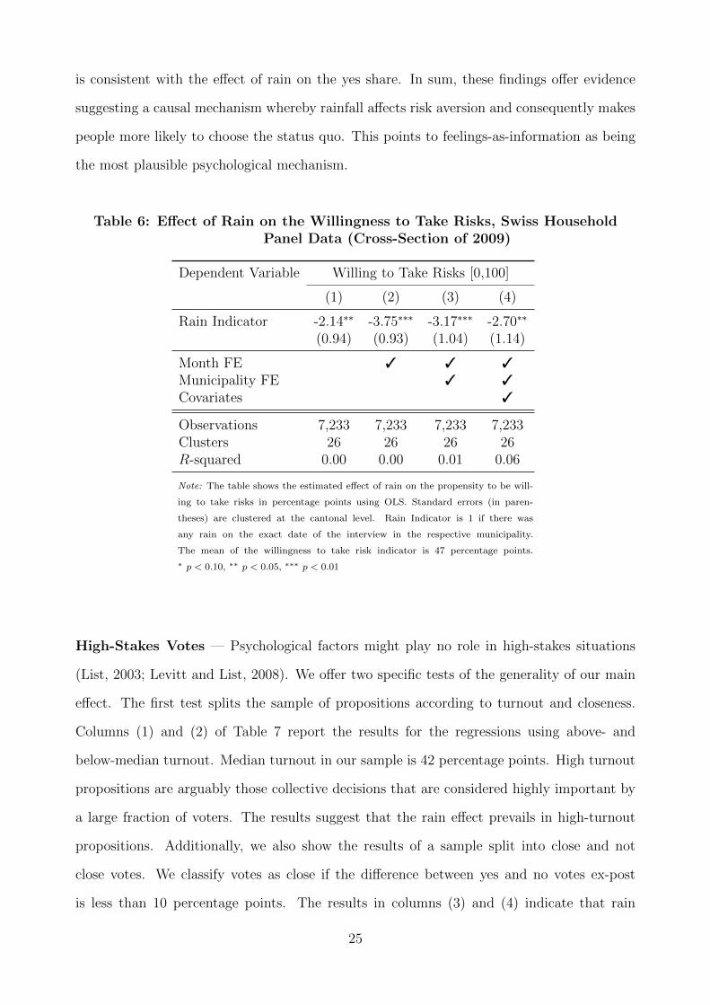
is consistent with the effect of rain on the yes share. In sum, these findings offer evidence

suggesting a causal mechanism whereby rainfall affects risk aversion and consequently makes

people more likely to choose the status quo. This points to feelings-as-information as being

the most plausible psychological mechanism.

Table 6: Effect of Rain on the Willingness to Take Risks, Swiss HouseholdPanel Data (Cross-Section of 2009)

Dependent Variable Willing to Take Risks [0,100]

(1) (2) (3) (4)

Rain Indicator -2.14∗∗ -3.75∗∗∗ -3.17∗∗∗ -2.70∗∗

(0.94) (0.93) (1.04) (1.14)

Month FE 3 3 3

Municipality FE 3 3

Covariates 3


Note: The table shows the estimated effect of rain on the propensity to be will-

ing to take risks in percentage points using OLS. Standard errors (in paren-

theses) are clustered at the cantonal level. Rain Indicator is 1 if there was

any rain on the exact date of the interview in the respective municipality.

The mean of the willingness to take risk indicator is 47 percentage points.

∗ p < 0.10, ∗∗ p < 0.05, ∗∗∗ p < 0.01

High-Stakes Votes — Psychological factors might play no role in high-stakes situations

(List, 2003; Levitt and List, 2008). We offer two specific tests of the generality of our main

effect. The first test splits the sample of propositions according to turnout and closeness.

Columns (1) and (2) of Table 7 report the results for the regressions using above- and

below-median turnout. Median turnout in our sample is 42 percentage points. High turnout

propositions are arguably those collective decisions that are considered highly important by

a large fraction of voters. The results suggest that the rain effect prevails in high-turnout

propositions. Additionally, we also show the results of a sample split into close and not

close votes. We classify votes as close if the difference between yes and no votes ex-post

is less than 10 percentage points. The results in columns (3) and (4) indicate that rain

25

decreases support for a change from the status quo in both close and not close propositions.

Overall, the results sustain that the effect of emotions on support for the status quo extends

to important political decisions.

Table 7: Sensitivity of the Rain Effect to High Turnout and Close Votes

Dependent Variable Share of Yes Votes [0-100]

High Turnout Low Turnout Close Votes Not Close Votes(1) (2) (3) (4)

Rain Indicator -1.26∗∗∗ -1.41∗∗ -1.08∗∗∗ -1.32∗∗

(0.36) (0.58) (0.34) (0.57)

Proposal FE 3 3 3 3

Municipality FE 3 3 3 3

Mun. Trends 3 3 3 3


Note: The table shows the estimated effect of rain on the share of yes votes in percentage points using OLS. Standarderrors (in parentheses) are clustered at the cantonal level. The rain Indicator is 1 for all rainy voting weekends. Highturnout corresponds to above median turnout. Median turnout is 42 percentage points. Close votes correspond to anex post difference in vote share of less than 10 percentage points. ∗ p < 0.10, ∗∗ p < 0.05, ∗∗∗ p < 0.01

Status Quo vs. Right-Wing Votes — We explore another alternative interpretation of

our results, namely that negative emotions increase the support for traditional and conser-

vative propositions. Since change is favored by the left-wing parties in some popular votes

and by the right-wing parties in others, we are able to separate the effect of emotions the

support for the status quo from the effect on traditionalist conservative positions.19 To do

this, we split our sample according to the party recommendations. If emotions increase the

likelihood that voters will vote for conservative propositions endorsed by a right-wing party,

we expect to find that rain has a positive rather than a negative effect for this subset of

propositions. Table A.9 in the Appendix shows the results for the different sample splits

according to the vote recommendations. The results suggest that rain decreases the share

of yes votes for all propositions independent of whether the proposals are supported by left-

19A prominent example for a policy change supported by the right-wing parties was the vote on asylumabuse in 2002, which demanded much stricter standards regarding asylum seekers. In about half of the votesin our sample, the right-wing parties supported a change from the status quo.

26

or right-wing parties. Thus, it seems that emotions affect the support for the status quo in

general, rather than the support for specific partisan policies.

Swing Voters — We would expect that citizens with less intense policy preferences, often

called swing voters, are particularly affected by transitory emotions.20 In order to identify

swing voters in popular votes, we predict the probability of voting yes for each voter based

on his or her individual characteristics. For these predictions, we use dummies for age,

gender, income, university degree, preferred party, ideology, average participation in votes,

as well as cantonal fixed effects. We then separate the electorate into terciles with respect

to the predicted propensity to vote yes. We thus have three groups, the status quo voters

(0.12 < P (Yes) < 0.44), the swing voters (0.44 ≤ P (Yes) ≤ 0.49) and the reformists

(0.49 < P (Yes) < 0.70).

For these three groups, we run the main regression. The results are presented in Ta-

ble A.10 in the Appendix. We observe that the swing voters are the ones who are sub-

stantially more likely to cast a yes vote rather than a no vote if it rains, while there are

no statistically significant effects on the other two groups. Consistent with this, we see the

largest absolute effect of rain on vote outcomes within municipalities that are in the middle

tercile with respect to their average share of yes votes.21

5 Conclusion

This study provides the first real-world evidence on the relationship between emotions and

preferences for the status quo. We use exogenous variation in rainfall to show that in-

dividuals who experience negative emotions are 1.2 percentage points less likely vote for

change. We explore several mechanisms. Our findings are most consistent with a theory

of feelings-as-information; that is, the notion that negative emotions lead to less optimistic

judgments (Schwarz, 2012).

20In the 1995 parliamentary elections, the share of swing voters was estimated to be around 33% (Lutz,2012).

21Note that we do not see statistically significant heterogeneity in turnout due to rainfall across the groups,either at the individual or at the municipal-level. Results available upon request.

27

The societal consequences of emotional choices can be substantial. Our simulation indi-

cates that emotions not just alter individual voting behavior, but may also sway aggregate

vote outcomes. A notable example is the referendum on Switzerland’s membership in the

European Economic Area in 1992. This proposal was rejected by a narrow margin of vot-

ers on a rainy weekend. Our results suggest that the voting outcome might well have been

swayed by positive emotions due to good weather.

This suggests that citizens are well advised to take important decisions on separate days.

Even if the decision maker were aware of the possibility of being influenced by rainfall, it

might be difficult to alleviate the effect of transitory emotions on behavior. The impact of

weather on voting outcomes also has implications for the agenda-setting power of govern-

ments. Anecdotal evidence suggests that the Scottish independence vote was intentionally

scheduled to a date with a pleasant weather forecast (Sayers, 2014).

The impact of emotions on the tendency to choose the status quo likely extends beyond

the domain of voting behavior. Kahneman, Knetsch and Thaler (1991) have pointed out that

the status quo effect is a well-known phenomenon in financial and insurance markets as well

as in other domains. Thus far, we have a very limited understanding of how emotions affect

the choice between change and the status quo in decision-making with respect to household

finances, health, education and labor supply (see, e.g., Haushofer and Fehr, 2014). Exploring

the impact of emotions in these domains appears to be a fruitful area for future research.

28

References

Arnold, Felix, and Ronny Freier. 2015. “The Partisan Effects of Voter Turnout: How Conservatives

Profit from Rainy Election Days.” DIW Berlin Discussion Paper No. 1463.

Augenblick, Ned, and Scott Nicholson. 2016. “Ballot Position, Choice Fatigue, and Voter Behavior.”

Review of Economic Studies, 83(2): 460–480.

Bassi, Anna. 2015. “Weather, Mood, and Voting: An Experimental Analysis of the Effect of Weather

Beyond Turnout.” mimeo.

Bassi, Anna, Riccardo Colacito, and Paolo Fulghieri. 2013. “O Sole Mio: An Experimental Analysis

of Weather and Risk Attitudes in Financial Decisions.” Review of Financial Studies, 26(7): 1824–1852.

Berggren, Niclas, Henrik Jordahl, and Panu Poutvaara. 2010. “The Looks of a Winner: Beauty and

Electoral Success.” Journal of Public Economics, 94(1-2): 8–15.

Busse, Meghan R., Devin G. Pope, Jaren C. Pope, and Jorge Silva-Risso. 2015. “The Psychological

Effect of Weather on Car Purchases.” Quarterly Journal of Economics, 130(1): 371–414.

Cameron, A. Colin, and Douglas L. Miller. 2015. “A Practitioner’s Guide to Cluster-Robust Inference.”

Journal of Human Resources, 50(2): 317–372.

Cameron, A. Colin, Jonah B. Gelbach, and Douglas L. Miller. 2011. “Robust Inference with Mul-

tiway Clustering.” Journal of Business & Economic Statistics, 29(2): 238–249.

Caplin, Andrew, and John Leahy. 2001. “Psychological Expected Utility Theory and Anticipatory

Feelings.” Quarterly Journal of Economics, 116(1): 55–79.

Card, David, and Gordon B. Dahl. 2011. “Family Violence and Football: The Effect of Unexpected

Emotional Cues on Violent Behavior.” Quarterly Journal of Economics, 126(1): 103–143.

Cohn, Alain, Jan Engelmann, Ernst Fehr, and Michel Andre Marechal. 2015. “Evidence for

Countercyclical Risk Aversion: An Experiment with Financial Professionals.” American Economic Review,

105(2): 860–885.

Conlin, Michael, Ted O’Donoghue, and Timothy J. Vogelsang. 2007. “Projection Bias in Catalog

Orders.” American Economic Review, 97(4): 1217–1249.

Cooperman, Alicia. 2016. “Randomization Inference with Rainfall Data: Using Historical Weather Pat-

terns for Variance Estimation.” mimeo.

Danziger, Shai, Jonathan Levav, and Liora Avnaim-Pesso. 2011. “Extraneous Factors in Judicial De-

cisions.” Proceedings of the National Academy of Sciences of the United States of America, 108(17): 6889–

92.

DellaVigna, Stefano. 2009. “Psychology and Economics: Evidence from the Field.” Journal of Economic

Literature, 47(2): 315–372.

DellaVigna, Stefano, John A. List, Ulrike Malmendier, and Gautam Rao. 2016. “Voting to Tell

Others.” Review of Economic Studies, forthcoming.

Dohmen, Thomas, Armin Falk, David Huffman, Uwe Sunde, Jurgen Schupp, and Gert G.

Wagner. 2011. “Individual Risk Attitudes: Measurement, Determinants, and Behavioral Consequences.”

Journal of the European Economic Association, 9(3): 522–550.

Elster, Jon. 1998. “Emotions and Economic Theory.” Journal of Economic Literature, 36(1): 47–74.

29

Elster, Jon. 1999. Alchemies of the Mind: Rationality and the Emotions. Cambridge University Press.

Eren, Ozkan, and Naci Mocan. 2016. “Emotional Judges and Unlucky Juveniles.” NBER Working Paper

No. 22611.

Federal Chancellery. 2005. “Briefliche Stimmabgabe - Analyse der eidg. Volksabstimmung vom 27. Novem-

ber 2005.” https://www.bk.admin.ch/aktuell/media/03238/index.html?lang=de&msg-id=4470.

Fernandez, Raquel, and Dani Rodrik. 1991. “Resistance to Reform: Status Quo Bias in the Presence

of Individual-Specific Uncertainty.” American Economic Review, 81(5): 1146–1155.

FORS - Swiss Foundation for Research in Social Sciences. 2014. “Vox Data: Standardized Post-

Referendum Surveys.” University of Lausanne.

Fowler, Anthony, and B Pablo Montagnes. 2015. “College Football, Elections, and False-Positive

Results in Observational Research.” Proceedings of the National Academy of Sciences of the United States

of America, 112(45): 13800–13804.

Fraga, Bernard, and Eitan Hersh. 2011. “Voting Costs and Voter Turnout in Competitive Elections.”

Quarterly Journal of Political Science, 5(4): 339–356.

Fujiwara, Thomas, Kyle C. Meng, and Tom Vogl. 2016. “Estimating Habit Formation in Voting.”

American Economic Journal: Applied Economics, forthcoming.

Hansford, Thomas G., and Brad T. Gomez. 2010. “Estimating the Electoral Effects of Voter Turnout.”

American Political Science Review, 104(02): 268–288.

Haushofer, Johannes, and Ernst Fehr. 2014. “On the Psychology of Poverty.” Science, 344(6186): 862–7.

Healy, Andrew J., Neil Malhotra, and Cecilia H. Mo. 2010. “Irrelevant Events Affect Voters’ Evalua-

tions of Government Performance.” Proceedings of the National Academy of Sciences of the United States

of America, 107(29): 12804–12809.

Healy, Andrew J., Neil Malhotra, and Cecilia H. Mo. 2015. “Determining False-Positives Requires

Considering the Totality of Evidence.” Proceedings of the National Academy of Sciences of the United

States of America, 112(48): 6591.

Hirshleifer, David, and Tyler Shumway. 2003. “Good Day Sunshine: Stock Returns and the Weather.”

Journal of Finance, 58(3): 1009–1032.

Hodler, Roland, Simon Luechinger, and Alois Stutzer. 2015. “The Effects of Voting Costs on the

Democratic Process and Public Finances .” American Economic Journal: Economic Policy, 7(1): 141–171.

Isen, Alice M. 2005. “Positive Affect.” In Handbook of Cognition and Emotion, Editors: Dalgleish, Tim

and Mick J. Power. 521–539. Chichester, UK:John Wiley & Sons, Ltd.

Johnson, Eric J., and Amos Tversky. 1983. “Affect, Generalization, and the Perception of Risk.” Journal

of Personality and Social Psychology, 45(1): 20–31.

Johnson, Eric J., and Daniel Goldstein. 2003. “Do Defaults Save Lives ?” Science, 302: 1338–1339.

Kahneman, Daniel, and Richard H. Thaler. 2006. “Anomalies: Utility Maximization and Experienced

Utility.” Journal of Economic Perspectives, 20(1): 221–234.

Kahneman, Daniel, Jack L. Knetsch, and Richard H. Thaler. 1991. “Anomalies: The Endowment

Effect, Loss Aversion, and Status Quo Bias.” Journal of Economic Perspectives, 5(1): 193–206.

30

Kamstra, Mark J., Lisa A. Kramer, and Maurice D. Levi. 2003. “Winter Blues: A SAD Stock

Market Cycle.” American Economic Review, 93(1): 324–343.

Lambert, G., C. Reid, D. Kaye, G. Jennings, and M. Esler. 2002. “Effect of Sunlight and Season on

Serotonin Turnover in the Brain.” The Lancet, 360(9348): 1840–1842.

Lee, David S. 2008. “Randomized Experiments from Non-Random Selection in U.S. House Elections.”

Journal of Econometrics, 142: 675–697.

Lerner, Jennifer S., Ye Li, Piercarlo Valdesolo, and Karim Kassam. 2015. “Emotion and Decision

Making.” Annual Review of Psychology, 66(33): 1–25.

Levitt, Steven D., and John A. List. 2008. “Homo Economicus Evolves.” Science, 319(5865): 909–910.

Lind, Jo T. 2015a. “Rainy Day Politics: An Instrumental Variables Approach to the Effect of Parties on

Political Outcomes.” mimeo.

Lind, Jo T. 2015b. “Spurious Weather Effects.” CESifo Working Paper Nr. 5365.

List, John A. 2003. “Does Market Experience Eliminate Market Anomalies?” Quarterly Journal of Eco-

nomics, 118(1): 41–71.

Loewenstein, George. 2000. “Emotions in Economic Theory and Economic Behavior.” The American

Economic Review, 90(2): pp. 426–432.

Loewenstein, George, Ted O’Donoghue, and Matthew Rabin. 2003. “Projection Bias in Predicting

Future Utility.” Quarterly Journal of Economics, 118(4): 1209–1248.

Lutz, Georg. 2012. “Eidgenossische Wahlen 2011, Wahlteilnahme und Wahlentscheid.” Selects - FORS.

Madestam, Andreas, Daniel Shoag, Stan Veuger, and David Yanagizawa-Drott. 2013. “Do Po-

litical Protests Matter? Evidence from the Tea Party Movement.” Quarterly Journal of Economics,

128(4): 1633–1685.

Marcus, George E. 2000. “Emotions in Politics.” Annual Review of Political Science, 3: 221–250.

MeteoSwiss - Federal Office of Meteorolgy and Climatology. 2015. “IDAWEB Weather Database.”

Bern: Federal Office of Meteorolgy and Climatology.

O’Donoghue, Ted, and Matthew Rabin. 2001. “Choice and Procrastination.” The Quarterly Journal

of Economics, 116(1): 121–160.

Samuelson, William, and Richard Zeckhauser. 1988. “Status Quo Bias in Decision Making.” Journal

of Risk and Uncertainty, 1(1): 7–59.

Sayers, Louise. 2014. “Scottish Independence: Are There Fair Weather Voters?” BBC Scotland.

Schwarz, Norbert. 2012. “Feelings-as-Information Theory.” In Handbook of Theories of Social Psychology:

Volume 1. 289–308. London:SAGE Publications Ltd.

SFS - Swiss Federal Statistical Office. 2015. Abstimmungsstatistik. Neuchatel.

Simonsohn, Uri. 2010. “Weather to Go to College.” Economic Journal, 120(543): 270–280.

Swissvotes - Database of Swiss Federal Referendums. 2012. Integraler Datensatz. Bern:Institute of

Political Science.

31

Appendix (For Online Publication)

A Additional Tables and Figures

Table A.1: Descriptive Statistics

Data Municipal Voting Data Postvote Survey Data1958–2014 1996–2006†

Mean SD Min. Max. Mean SD Min. Max.

Yes Share in %-Points 46.59 20.76 0 100 46.50 49.88 0 100Rain Indicator 0.55 0.49 0 1 0.70 0.46 0 1Rain in mm 2.67 5.78 0 104.50 5.25 7.23 0 64.50Turnout 43.58 13.26 0.16 100Postal Voting Dummy 0.49 0.49 0 1Ballot Box Voters 0.38 0.49 0 1Mail Voters 0.61 0.49 0 1

Observations 862,670 29,510

Note: †There is no municipal identifier available for the year 1997. Therefore we do not use this year.

Table A.2: Effect of Rain on the Share of Yes Votes in Percentage Points,Variants of Fixed Effects


(1) (2) (3) (4)

Rain Indicator -1.25∗∗∗ -1.27∗∗∗ -1.20∗∗∗ -1.31∗∗∗

(0.40) (0.41) (0.37) (0.43)

Proposal FE 3 3 3 3

Municipality FE 3 3

Mun. Trends 3 3 3

Mun. Trends: Quadratic 3 3

Mun. Trends: Cubic 3

Mun. x Month FE 3

Mun. x Year FE 3


Note: The table shows the estimated effect of rain on the share of yes votes in percentage

points using OLS. Standard errors (in parentheses) are clustered at the cantonal level. The

rain indicator is 1 for all rainy voting weekends. ∗ p < 0.10, ∗∗ p < 0.05, ∗∗∗ p < 0.01

32

Table A.3: Effect of Rain on the Share of Yes Votes in Percentage Points, Clus-tering of Standard Errors

Dependent Variable Share of Yes Votes Voted Yes(Municipal Voting Data) (Individual Voting Data)

(1) (2) (3) (4) (5) (6)

Rain Indicator -1.24∗∗∗ -1.24∗∗∗ -1.24∗∗∗ -3.15∗∗ -3.15∗∗ -3.15∗

(0.41) (0.05) (0.41) (1.32) (1.54) (1.53)

Cluster:Vote Weekend 3 3

Municipality 3 3

Mun.×Vote Weekend† 3 3

Clusters 164 2,538 164×2,538 22 1,355 22×1,355



Mun. Trends 3 3 3

Covariates 3 3 3

Observations 862,670 862,670 862,670 29,510 29,510 29,510R-squared 0.72 0.72 0.72 0.21 0.21 0.21

Note: The table shows the estimated effect of rain on the share of yes votes (columns 1 to 3) or the propensity tovote yes (columns 4 to 6) in percentage points using OLS. Standard errors (in parentheses) are clustered as indicated.†Community×Vote Weekend means that clustering is allowed in both dimensions, that is it allows for twoway clus-tering as specified by (Cameron, Gelbach and Miller, 2011). The rain indicator is 1 for all rainy voting weekends.∗ p < 0.10, ∗∗ p < 0.05, ∗∗∗ p < 0.01

Table A.4: Effect of Rain on Turnout in Percentage Points by Past Turnoutand Knowledge, Postvote Survey Data 1996-2006

Dependent Variable Turnout [0,100]

Distant Marginal Always Knowledge No KnowledgeVoters Voters Voters

(1) (2) (3) (4) (5)

Rain Indicator -3.98 1.22 -0.33 1.56 -1.81(3.11) (2.28) (1.27) (1.65) (1.50)

Mean Yes Share 39.01 44.16 47.84 46.52 44.81

Proposal FE 3 3 3 3 3

Municipality FE 3 3 3 3 3

Covariates 3 3 3 3 3

Observations 2,542 6,068 7,741 7,387 7,840Clusters 26 26 26 26 26R-squared 0.42 0.27 0.23 0.26 0.28

Note: The table shows the estimated effect of rain on the propensity to vote using OLS. Standard er-

rors (in parentheses) are clustered at the cantonal level. The rain indicator is 1 for all rainy vot-

ing weekends. Average turnout: 65.16%, maximum number of observations containing turnout: 19,794.

∗ p < 0.10, ∗∗ p < 0.05, ∗∗∗ p < 0.01

33

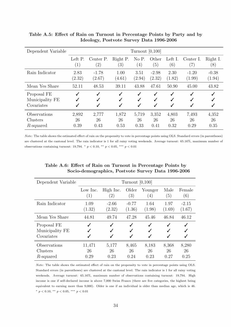
Table A.5: Effect of Rain on Turnout in Percentage Points by Party and byIdeology, Postvote Survey Data 1996-2006


Left P. Center P. Right P. No P. Other Left I. Center I. Right I.(1) (2) (3) (4) (5) (6) (7) (8)

Rain Indicator 2.83 -1.78 1.00 3.51 -2.98 2.30 -1.20 -0.38(2.32) (2.67) (4.61) (2.94) (2.32) (1.82) (1.99) (1.94)

Mean Yes Share 52.11 48.53 39.11 43.88 47.61 50.90 45.00 43.82

Proposal FE 3 3 3 3 3 3 3 3

Municipality FE 3 3 3 3 3 3 3 3

Covariates 3 3 3 3 3 3 3 3

Observations 2,892 2,777 1,872 5,719 3,352 4,803 7,493 4,352Clusters 26 26 26 26 26 26 26 26R-squared 0.39 0.43 0.53 0.33 0.41 0.32 0.29 0.35

Note: The table shows the estimated effect of rain on the propensity to vote in percentage points using OLS. Standard errors (in parentheses)

are clustered at the cantonal level. The rain indicator is 1 for all rainy voting weekends. Average turnout: 65.16%, maximum number of

observations containing turnout: 19,794. ∗ p < 0.10, ∗∗ p < 0.05, ∗∗∗ p < 0.01

Table A.6: Effect of Rain on Turnout in Percentage Points bySocio-demographics, Postvote Survey Data 1996-2006


Low Inc. High Inc. Older Younger Male Female(1) (2) (3) (4) (5) (6)

Rain Indicator 1.09 -2.66 -0.77 1.64 1.97 -2.15(1.32) (2.32) (1.36) (1.98) (1.69) (1.67)

Mean Yes Share 44.81 49.74 47.28 45.46 46.84 46.12



Covariates 3 3 3 3 3 3


Note: The table shows the estimated effect of rain on the propensity to vote in percentage points using OLS.

Standard errors (in parentheses) are clustered at the cantonal level. The rain indicator is 1 for all rainy voting

weekends. Average turnout: 65.16%, maximum number of observations containing turnout: 19,794. High

income is one if self-declared income is above 7,000 Swiss Francs (there are five categories, the highest being

equivalent to earning more than 9,000). Older is one if an individual is older than median age, which is 46.

∗ p < 0.10, ∗∗ p < 0.05, ∗∗∗ p < 0.01

34

Table A.7: Sensitivity of the Rain Effect Conditional on Partisan Preferences ofMunicipalities

Dependent Variable Share of Yes Votes [0–100] Turnout [0–100]

Left Center Right Left Center Right(1) (2) (3) (4) (5) (6)

Rain Indicator -0.85∗∗∗ -1.04∗∗∗ -1.37∗∗ -0.29 -0.48 -0.38(0.30) (0.34) (0.55) (0.27) (0.36) (0.23)



Mun. Trends 3 3 3 3 3 3


Note: The table shows the estimated effect of rain on the share of yes votes (columns 1 to 3) or turnout (columns4 to 6) in percentage points using OLS. Standard errors (in parentheses) are clustered at the cantonal level. Therain indicator is 1 for all rainy voting weekends. Classification according to above median share of right, centeror left-wing parties in the last national council election. ∗ p < 0.10, ∗∗ p < 0.05, ∗∗∗ p < 0.01

Table A.8: Robustness of the Rain Effect to Change in Information Sources

Dependent variable Voted Yes Individual Knowledge†

(1) (2) (3)All Voters All Voters Ballot Box Voters

Rain Indicator -3.25∗∗ 0.56 1.79(1.31) (2.88) (4.45)

Information Channel 3

Proposal FE 3 3 3

Municipality FE 3 3 3

Covariates 3 3 3

Observations 26,459 28,628 10,776Observations 26 26 26R-squared 0.22 0.27 0.43

Note: The table shows the estimated effect of rain on the propensity to vote yes (column 1)or the propensity to know the title of the proposition (columns 2 and 3) in percentage pointsusing OLS. Standard errors (in parentheses) are clustered at the cantonal level. The rainindicator is 1 for all rainy voting weekends. Information channel includes dummies for in-formation sources a voter used. †Knowledge is 100 if the voter knows the title of a propo-sition and 0 otherwise. We only include voters that voted at the ballot box in column (3).∗ p < 0.10, ∗∗ p < 0.05, ∗∗∗ p < 0.01

35

Table A.9: Effect of Rain on the Share of Yes Votes by Party Recommendation


Left Right(1) (2)

Rain Indicator -0.96∗∗∗ -1.17∗∗

(0.30) (0.51)

Proposal FE 3 3

Municipality FE 3 3

Mun. Trends 3 3

Observations 335,957 526,713Clusters 26 26R-squared 0.69 0.64

Note: The table shows the estimated effect of rain on the share ofyes votes in percentage points using OLS. Standard errors (in paren-theses) are clustered at the cantonal level. The rain indicator is 1 forall rainy voting weekends. Right corresponds to a vote recommenda-tion to vote yes of the SVP (right-wing) or the FDP (center-right).Left corresponds to all votes where there was no such recommendation.∗ p < 0.10, ∗∗ p < 0.05, ∗∗∗ p < 0.01

Table A.10: Sensitivity of the Rain Effect Conditional on the Propensity to VoteYes

Dependent Variable Voted Yes [0,100] Share of Yes Votes [0–100]

Status Quo Swing Reformist Status Quo Swing ReformistVoter Voter Voter Mun. Mun. Mun.(1) (2) (3) (4) (5) (6)

Rain Indicator 2.23 -6.72∗∗ -0.78 -0.87∗ -1.32∗∗ -0.91∗∗∗

(2.17) (2.54) (2.47) (0.45) (0.58) (0.30)



Mun. Trends 3 3 3 3 3 3


Note: The table shows the estimated effect of rain on the propensity to vote yes (columns 1 to 3) or the share of yesvotes (columns 4 to 6) in percentage points using OLS. Standard errors (in parentheses) are clustered at the cantonal level.The rain indicator is 1 for all rainy voting weekends. Propensities of yes votes at the individual-level: status quo voters(0.12 < P (Yes) < 0.44), swing voters (0.44 ≤ P (Yes) ≤ 0.49) and reformists (0.49 < P (Yes) < 0.70). Average share of yes votesat the municipal-level: 0.32 < Share(Y es) < 0.45, 0.45 ≤ Share(Y es) ≤ 0.48 and 0.48 < Share(Y es) < 0.59. ∗ p < 0.10, ∗∗

p < 0.05, ∗∗∗ p < 0.01

36

Figure A.1: Distribution of Votes and Rain over Months

0.1

.2.3

.4.5

.6.7

.8.9

1

Shar

e of

Rai

ny V

ote

Wee

kend

s

JanFeb

MarApr

MayJun

JulAug

SepOct

NovDec

Month

Municipalities with Rainfall

05

1015

2025

30

Num

ber o

f Vot

edat

esJan

FebMar

AprMay

JunJul

AugSep

OctNov

Dec

Month

Vote Weekends per Month

Note: The figures show the distribution of voting weekends over months and the share of communities withrainy voting weekends by month.

Figure A.2: Map of the Share of Yes Votes

Note: The figure shows the average share of yes votes by municipality.

37

Figure A.3: Map of the Share of Rainy Vote Weekends

Note: The figure shows the share of rainy voting weekends. Note that the clusters with the high share of rainyweekends lie in the Alps and over the Jura mountains.

Figure A.4: Distribution of the Share of Rainy Vote Weekends over Municipali-ties

05

1015

20Pe

rcen

tage

of M

unic

ipal

ities

.2 .3 .4 .5 .6 .7 .8 .9 1Share of Rainy Vote Weekends

Note: The blue line indicates the average share of rainy voting weekends which is 55%.

38

Figure A.5: Share of Communities with Rainfall by Date

.

Figure A.6: Map of Weather Stations

Note: The figure shows the weather stations we use for our analysis.

39

Figure A.7: Flexible Relationship between Rain in Terciles and Share of YesVotes in Percentage Points, Postvote Survey Data

-10

-8-6

-4-2

02

Effe

ct o

f Rai

n (in

Per

c. P

oint

s)

Med.-Heavy Rain(4.3-64.5]

Light Rain(0.8-4.3]


Rain in mm

Note: The figure shows coefficient estimates, 95% confidence intervals (thin line) and 90% confidence intervals(thick line) for the effect of rain on the share of yes votes in percentage points using postvote survey data. Thereference category is zero rainfall.

Figure A.8: Flexible Relationship between Rain in Quintiles and Share of YesVotes in Percentage Points, Municipal Data

-6-5

-4-3

-2-1

01

Effe

ct o

f Rai

n (in

Per

c. P

oint

s)

Quint. 5(8.0-105]

Quint. 4(3.3-8.1]

Quint. 3(1.3-3.3]

Quint. 2(0.3-1.3]

Quint. 1(0.0-0.3]

Rain in mm

Note: The figure shows coefficient estimates, 95% confidence intervals (thin line) and 90% confidence intervals(thick line) for the effect of rain on the share of yes votes in percentage points using municipal data. The dotsare retreived from regression model (4) in Table 2 with indicator variables for the five quintiles of rainfall insteadof one indicator. The reference category is zero rainfall.

40

Figure A.9: Flexible Relationship between Rain in Quintiles and Turnout in Per-centage Points, Municipal Data

-6-5

-4-3

-2-1

01

Effe

ct o

f Rai

n (in

Per

c. P

oint

s)

Quint. 5(8.0-105]

Quint. 4(3.3-8.1]

Quint. 3(1.3-3.3]

Quint. 2(0.3-1.3]

Quint. 1(0.0-0.3]

Rain in mm

Note: The figure shows coefficient estimates, 95% confidence intervals (thin line) and 90% confidence intervals(thick line) for the effect of rain on the share of yes votes in percentage points using municipal data. The dotsare retrieved from a regression of turnout on indicator variables for the five quintiles of rainfall while controllingfor municipality fixed effects, proposal fixed effects and cantonal trends. The reference category is zero rainfall.

Figure A.10: Effect of Rain on Turnout vs. Effect of Rain on Share of Yes Votes,Municipal Data

-3-2

-10

1

Effe

ct o

f Rai

n (in

Per

c. P

oint

s)

Quint. 5(8.0-105]

Quint. 4(3.3-8.1]

Quint. 3(1.3-3.3]

Quint. 2(0.3-1.3]

Quint. 1(0.0-0.3]

Rain in mm

Effect on Turnout Effect on Yes Share

Note: The figure shows coefficient estimates for the effect of rain on turnout in percentage points (black dots)and on the yes share in percentage points (blue triangles) using municipal data. The dots are retrieved fromregression model (4) in Table 1 using turnout or the yes share as dependent variable and with indicator variablesfor quintiles of rainfall instead of one indicator. The reference category is zero rainfall.

41

Figure A.11: Selection Corrected Coefficients, Postvote Survey Data

-6-5

-4-3

-2-1

01

Cor

rect

ed E

ffect

of R

ain

(in P

erc.

Poi

nts)

Past T

urnou

t

Knowled

ge

Parties

Ideolo

gies

Incom

eAge

Gende

r

Group

Note: The figure shows turnout corrected coefficient estimates, 95% confidence intervals (thin line) and 90%confidence intervals (thick line) for the effect of rain on the share of yes votes in percentage points with postvotesurvey data. The baseline estimate is shown with the blue solid line. The depicted coefficients are correctedby heterogeneous selection within groups of voters, for instance conditional on their past turnout behavior.Marginal voters are less likely to vote if it rains and are more likely to vote no – the opposite holds true for morefrequent voters. Accordingly the coefficient estimate is adjusted downwards, since we likely underestimate thetrue rain effect.

Figure A.12: Sensitivity to Sample Selection by Party Preferences

-8-7

-6-5

-4-3

-2-1

01

2Ef

fect

of R

ain

(in P

erc.

Poi

nts)

CSPCVP

EVPFDP

FPS

Gruene Ld

ULe

ga LPS

PdA SDSPS

SVPFrap GB

LdU

Other

Severa

l

Politic

al, no

party

No part

y

No Dec

ision NA

Party Left Out

Note: The figure shows coefficient estimates, 95% confidence intervals (thin line) and 90% confidence intervals(thick line) for the effect of rain on the share of yes votes in percentage points with postvote survey data. Theestimate resulting from all data is shown with the blue solid line.

42

Figure A.13: Sensitivity to Sample Selection by Ideology

-8-7

-6-5

-4-3

-2-1

01

2Ef

fect

of R

ain

(in P

erc.

Poi

nts)

Extrem

e Left 1 2 3 4

Center 6 7 8 9

Extrem

e Righ

t

Ideology Left Out

Note: The figure shows coefficient estimates, 95% confidence intervals (thin line) and 90% confidence intervals(thick line) for the effect of rain on the share of yes votes in percentage points with postvote survey data. Theestimate resulting from all data is shown with the blue line.

Figure A.14: Flexible Relationship Between Rain in Terciles and the Willingnessto Take Risks

-12

-8-4

04

Effe

ct o

f Rai

n (in

Per

c. P

oint

s)


Light Rain(0.8-4.3]


Rain in mm

Note: The figure shows coefficient estimates, 95% confidence intervals (thin line) and 90% confidence intervals(thick line) for the effect of rain on the propability that an individual is willing to take risks based on data fromthe Swiss Household Panel. The reference category is zero rainfall.

43

B Econometric Model for Individual Voting Decisions

In a similar vein as with the municipal data, we estimate the effect of rain in the propensity ofan individual to vote yes using the postvote survey data. We use the following specification:

Yijp = ηj + δp + αRainjp +X ′ijpβ + εijp, (2)

where i indexes voters, j indexes municipalities and p indexes propositions; ηj is a mu-nicipal fixed effect, Rainjp is a dummy that captures rain in municipality j when voters voteon proposition p; X ′ijp is a matrix of individual-level covariates; εijp is an idiosyncratic errorterm. In our baseline specification, we include dummies capturing the following covariates:gender, age, income categories and holding a university degree.

44

rain, emotions and voting for the status quoftp.iza.org/dp10350.pdf · november 2016 abstract rain,...

Documents