Noname manuscript No.(will be inserted by the editor)

General Default Logic

Yi Zhou · Fangzhen Lin · Yan Zhang

the date of receipt and acceptance should be inserted later

Abstract In this paper, we propose general default logic, which extends Reiter’s de-

fault logic by adding rule connectives like disjunction in logic programming, and Fer-

raris’s general logic program by allowing arbitrary propositional formulas to be the

base in forming logic programs. We show the usefulness of this logic by applying it to

formalize rule constraints, generalized closed world assumptions, and conditional de-

faults. We study the relationship between general default logic and other nonmonotonic

formalisms such as Lin and Shoham’s logic of GK, Moore’s auto-epistemic logic etc.,

and investigate its normal form under a notion of strong equivalence. We also address

the computational properties related to our logic.

Keywords Nonmonotonic Logic · Answer Set Program · Default Logic · Auto-

epistemic Logic

1 Introduction

Answer set semantics for logic programs has been emerged as a promising approach

for knowledge representation and deductive database in recent decades. Answer set

programming started from Gelfond and Lifschitz’s stable model semantics for logic

This paper is an extended version of the authors’ LPNMR’07 and NMR’08 paper.

Yi ZhouIntelligent Systems LabSchool of Computing and MathematicsUniversity of Western Sydney, NSW, AustraliaE-mail: yzhou@scm.uws.edu.au

Fangzhen LinDepartment of Computer ScienceHong Kong University of Science and Technology, HongKongE-mail: flin@cse.edu.hk

Yan ZhangIntelligent Systems LabSchool of Computing and MathematicsUniversity of Western Sydney, NSW, AustraliaE-mail: yan@scm.uws.edu.au

2

programs with negation as failure [14], which is known as normal logic programs. In a

normal logic program, the head of a rule must be an atom. If one allows disjunctions

of atoms in the head of rule, then one obtains what has been called disjunctive logic

programs [15]. However, in disjunctive logic programs, the disjunctions are allowed only

in the head of a rule. It cannot occur in the body of a rule nor can it be nested. This

limitation in the use of disjunction has been addressed by Lifschitz et al. [29], Pearce

[41] and recently by Ferraris [12].

Ferraris defined logic programs that look just like propositional formulas but are

interpreted according to a generalized stable model semantics. In other words, in these

formulas called general logic programs, negations are like negation-as-failure; impli-

cations are like rules; and disjunctions are like those in disjunctive logic programs.

They are essentially different from those corresponding classical connectives. We call

these connectives rule connectives, including negation as failure, rule implication, rule

conjunction and rule disjunction.

The differences between negation as failure and classical negation are well discussed

in the literature [6,15]. The former means ”unknown” while the latter means ”false”.

For instance, the program {¬p, q ← ¬r} has a unique answer set {¬p}. In contrast, the

program {notp, q ← notr} also has a unique answer set, which is {q}. It has also been

shown that both classical negation and negation as failure are needed simultaneously

in some cases in knowledge representation [15].

However, the relationships between other rule connectives and corresponding classi-

cal connectives remain unclear. Here, we focus on disjunctions. One difference between

rule disjunction and classical disjunction is that the former requires minimality while

the latter does not. For instance, the disjunctive logic program p | q ← has two answer

sets {p} and {q}, but the propositional formula p ∨ q has three models1 {p}, {q}, and

{p, q}. Another difference is that rule disjunction is deterministic choice while classi-

cal disjunction is nondeterministic choice. For instance, the disjunctive logic program

p | ¬p has two answer sets {p} and {¬p}, which means that the truth (falsity) of p

is confirmed. On the other hand, the propositional formula p ∨ ¬p is equivalent to >,

which represents no information about p. The following example may explain more on

the differences between these two kinds of disjunctions:

Example 1 Suppose that we are reasoning about a shopping agent A. The agent wants

to buy iodine. There are two cases:

1. Another agent B told to A that supermarket or pharmacy have iodine to sell. But B wasnot sure which one does.

2. Another agent C told to A which store has iodine to sell. But to our knowledge, we arenot sure this store is supermarket or pharmacy.

To formalize our information about A, the disjunction in the first sentence should be

formalized as classical disjunction while the disjunction in the second sentence should

be formalized as rule disjunction. One difference is that, for the agent A, the former is

a nondeterministic choice while the latter is a deterministic choice. We can formalize

our information as follows:

1. HasIodine(supermarket) ∨HasIodine(pharmacy).

2. HasIodine(supermarket) |HasIodine(pharmacy).

Of course, if A knows which store has iodine, she will go to buy it. However, if she

is not sure which store has iodine, she would hesitate a moment. Formally,

1 We identify a model with the set of atoms that are true in the model.

3

3. BoughtIodine ← HasIodine(supermarket), not ¬BoughtIodine.

4. BoughtIodine ← HasIodine(pharmacy), not ¬BoughtIodine.

5. Hesitate ← not HasIodine(supermarket), not HasIodine(pharmacy).

Example 1 also indicates that both rule disjunction and classical disjunction are needed

when representing incomplete information. They represent different senses of disjunc-

tions.

Hence, a natural question is whether answer set programming can be extended with

also connectives from classical logic. The family of default logics may play such a role.

Default logics and answer set programming are closely related. Gelfond and Lifschitz

[15] showed that answer set semantics for normal logic programs can be embedded in

to Reiter’s default logic [42] with a simple translation. This result means that Reiter’s

default logic allows both connectives from logic programs and classical connectives.

However, it does not allow rule disjunctions. Gelfond et al. [16] extended Reiter’s

default logic into disjunctive default logic by allowing the head of default rules to

be rule disjunctions of propositional formulas. They also showed that the answer set

semantics of disjunctive logic programs can be embedded in disjunctive default logic.

Turner [46] introduced nested default logic, which is a generalization of disjunctive

default logic as well as nested logic programming. Thus, a second question arises:

whether is there such a default logic corresponding to Ferraris’s answer semantics for

general logic programs?

This paper answers these two questions positively. We introduce a logic, which is

both an extension of Ferraris’s general logic programming and Reiter’s default logic. In

this logic, rules are defined as any compositions of classical propositional formulas and

rule connectives. We define the model semantics as well as the extension semantics for

rules. Similar to default logic, an extension (model) of a rule is a propositional theory.

We also show that this logic is a generalization of all the default logics and answer set

semantics for logic programs mentioned earlier. Since this logic is a generalized version

of default logics corresponding to Ferraris’s stable model semantics for general logic

programs, we call this logic general default logic.

The combination of classical logic and rules is not a new idea in the KR community.

CLASSIC [4] is an early description logic allowing simple monotonic rules. Donini

et al. [8] combined Datalog with description logic ALC. However, their combination

are dealing with neither negation as failure nor rule disjunction. This limitation was

addressed by Rosati [43]. Recently, in order to bridge the gap between the ontology

layer and rule layer in the Semantic Web layer cake [1], a large number of combinations

of description logics and rules [21,23,11] have been proposed. Although these works

are based on tractable fragments of first order logic rather than propositional logic, we

believe that a comprehensive study of the combination in propositional case would be

very useful to this goal.

2 Defining the Logic

In this section, we define our logic that allows both classical connectives and connectives

from answer set programming. We then study some semantic properties of R.

4

2.1 Syntax

Let Atom be a set of atoms, which are also called propositional variables. By L we

mean the classical propositional language defined recursively by Atom and classical

connectives ⊥, ¬, → as follows:

F ::= ⊥ | p | ¬F | F → F,

where p ∈ Atom. >, F ∧G, F ∨G and F ↔ G are considered as shorthand of ⊥ → ⊥,

¬(F → ¬G), ¬F → G and (F → G) ∧ (G → F ) respectively, where F and G are

formulas in L. Formulas in L are called facts2. The satisfaction relation |= between a

set of facts and a fact is defined as usual. A theory T is a set of facts which is closed

under classical entailment. Let Γ be a set of facts, Th(Γ ) denotes the logic closure of

Γ under classical entailment. We write Γ to denote the theory Th({Γ}) if it is clear

from the context. For instance, we write ∅ to denote the theory of all tautologies; we

write {p} to denote the theory of all logic consequences of p. We say that a theory T

is inconsistent if there is a fact F such that T |= F and T |= ¬F , otherwise, we say

that T is consistent.

We introduce a set of new connectives, called rule connectives. They are − for

negation as failure or rule negation, ⇒ for rule implication, & for rule conjunction, |for rule disjunction3 and ⇔ for rule equivalence respectively. We define a propositional

language R recursively by facts and rule connectives as follows:

R ::= F | R ⇒ R | R & R | R |R,

where F is a fact. −R and R ⇔ S are considered as shorthand of R ⇒ ⊥ and (R ⇒S)& (S ⇒ R) respectively, where R and S are formulas in R. Formulas in R are called

rules. Particularly, facts are also rules. A rule base ∆ is a set of rules.

The order of priority for these connectives are

{¬} > {∧,∨} > {→,↔} > {−} > {& , | } > {⇒,⇔}.

For example, −p∨¬p ⇒ q is a well defined rule, which denotes the rule (−(p∨(¬p))) ⇒q. Both ¬p∨ p and ¬p | p are well defined rules. The former is also a fact but the latter

is not. However, ¬(p | p) is not a well defined rule.

We define the subrule relationship between two rules recursively as follows:

1. R is a subrule of R;

2. R and S are subrules of R ⇒ S;

3. R and S are subrules of R & S;

4. R and S are subrules of R | S,

where R and S are rules. Thus, clearly, R is a subrule of −R. For example, p is a

subrule of ¬p | p but not a subrule of ¬p ∨ p.

2 In logic programming, facts and rules often denote propositional variables and declarativesentences. Here, as an generalization of logic programming, we lift these two notions to denotepropositional formulas and well defined formula in the rule language respectively.

3 These connectives are sometimes also denoted by not, ←, , and ; respectively in answerset programming.

5

2.2 Basic semantics

We define the satisfaction relation |=R between theories and rules inductively:

– If R is a fact, then T |=R R iff T |= R.

– T |=R R & S iff T |=R R and T |=R S;

– T |=R R | S iff T |=R R or T |=R S;

– T |=R R ⇒ S iff T 6|=R R or T |=R S.

Thus, T |=R −R iff T |=R R → ⊥ iff T 6|=R R or T |=R ⊥. If T is consistent,

then T |=R −R iff T 6|=R R. If T is inconsistent, then for every rule R, T |=R R.

T |=R R ⇔ S iff T |=R (R ⇒ S) & (S ⇒ R) iff T |=R R ⇒ S and T |=R S ⇒ R.

We say that T satisfies R, also T is a model of R iff T |=R R. We say that T

satisfies a rule base ∆ iff T satisfies every rule in ∆. We say that two rule bases are

weakly equivalent if they have the same set of models.

For example, let T be ∅. T is a model of ¬p ∨ p, but T is not a model of ¬p | p.

This example also shows a difference between the two connectives ∨ and | . As another

example, T is a model of −p but not a model of ¬p. This example also shows a difference

between the two connectives ¬ and −.

2.3 Extension

Let T be a theory and R a rule in R. The reduction of R relative to T , denoted by RT ,

is the formula obtained from R by replacing every maximal subrules of R which is not

satisfied by T with ⊥. It can also be defined recursively as follows:

– If R is a fact, then RT =

{R if T |=R R

⊥ otherwise,

– If R is R1 ¯ R2, then RT =

{RT

1 ¯RT2 if T |=R R1 ¯R2

⊥ otherwise, where ¯ is & , ⇔, |

or ⇒.

Thus, if R is −S and T is consistent, then RT =

{⊥ if T |=R S

> otherwise.

Let T be a theory and ∆ a rule base, the reduction of ∆ relative to T , denoted by

∆T , is the set of all the reductions of rules in ∆ on T .

For example, let T be {p}. The reduction of −p ⇒ q relative to T is ⊥ ⇒ ⊥, which

is weakly equivalent to >. The reduction of p | q relative to T is p. The reduction of

p∨ q relative to T is p∨ q. This example also shows that although two rules are weakly

equivalent (i.e. −p ⇒ q and p | q), their reductions relative to a same theory might not

be weakly equivalent.

Definition 1 Let T be a theory and ∆ a rule base. We say that T is an extension of

F iff:

1. T |=R ∆T .

2. There is no theory T1 such that T1 ⊂ T and T1 |=R ∆T .

It is clear that if ∆ is a set of facts, then ∆ has exactly one extension, which is the

deductive closure of itself.

Example 2 Consider the rule base ∆1 = {−p ⇒ q}.

6

– Let T1 be ∅. The reduction of ∆1 relative to T1 is {⊥}. T1 is not a model of ∆T11 .

Hence, T1 is not an extension of ∆1.

– Let T2 be {p}. The reduction of ∆1 relative to T2 is ⊥ ⇒ ⊥. T2 is a model of ∆T21 .

But ∅ is also a model of ∆T21 and ∅ ⊂ T2. Hence, T2 is not an extension of ∆1.

– Let T3 be {q}. The reduction of ∆1 relative to T3 is > ⇒ q, which is weakly

equivalent to q. T3 is a model of q and there is no proper subset of T3 which is also

a model of q. Hence, T3 is an extension of ∆1.

– Let T4 be {¬p ∧ q}. The reduction of ∆1 relative to T4 is > ⇒ q, which is also

weakly equivalent to q. T4 is a model of ∆T41 . But {q} is also a model of ∆T4

1 . Hence

T4 is not an extension of ∆1.

– We can examine that the only extension (under classical equivalence) of ∆1 is T3.

Similarly, p | q has two extensions: {p} and {q}, while p ∨ q has a unique extension

{p ∨ q}. This example shows that although two rules are weakly equivalent, their

extensions might not be the same (i.e., −p ⇒ q and p | q).

Example 3 Consider the rule base ∆2 = {p, r | p ∨ q}.– Let T1 be ∅. The reduction of ∆2 relative to T1 is {⊥,>}. T1 is not a model of

∆T12 . Hence, T1 is not an extension of ∆2.

– Let T2 be {p}. The reduction of ∆2 relative to T2 is p,⊥. T2 is not a model of ∆T22 .

Hence, T2 is not an extension of ∆2.

– Let T3 be {p, r}. The reduction of ∆2 relative to T3 is p, r. Hence, T3 is an extension

of ∆2.

– We can examine that the only extension (under classical equivalence) of ∆2 is T3.

Example 4 (Example 1 continued) Recall that the example presented in the introduc-

tion section. Reformulate those information in general default logic:

1. HasIodine(supermarket) ∨HasIodine(pharmacy).

2. HasIodine(supermarket) |HasIodine(pharmacy).

3. HasIodine(supermarket) & − ¬BoughtIodine ⇒ BoughtIodine.

4. HasIodine(pharmacy) & − ¬BoughtIodine ⇒ BoughtIodine.

5. −HasIodine(supermarket) & −HasIodine(pharmacy) ⇒ Hesitate.

We can conclude that 1, 3 − 5 has a unique extension {HasIodine(supermarket) ∨HasIodine(pharmacy), Hesitate} while 2, 3−5 has two extensions {HasIodine(supermarket), BoughtIodine}and {HasIodine(pharmacy), BoughtIodine}. Suppose that we have a query to ask

whether the shopping agent got what she wants, in the first case the answer should be

”unknown” while in the second case the answer should be ”yes”.

2.4 Properties

The following proposition shows that some of the relationships among rule connectives

from the basic semantics level.

Proposition 1 Let T be a theory and R, S two rules in R.

1. T |=R −−R iff T |=R R.

2. T |=R −(R & S) iff T |=R −R | − S.

3. T |=R −(R | S) iff T |=R −R & − S.

7

4. T |=R R ⇒ S iff T |=R −R | S.

Proof These assertions follow directly from the definitions. As an example, we prove

only assertion 2 here. According to the definition, T |=R −(R & S) iff T is not a model

of R & S, which holds iff a) T is not a model of R or b) T is not a model of S. On the

other hand, T |=R −R | −S iff a) T is a model of −R or b) T is a model of −S, which

holds iff a) T is not a model of R or b) T is not a model of S. Hence, assertion 2 holds.

We are also interested in the relationships between classical connectives and corre-

sponding rule connectives.

Proposition 2 Let F and G be two facts and T a theory.

1. T is a model of F ∧G iff T is a model of F & G.

2. If T is a model of F |G, then T is a model of F ∨G.

3. If T is a model of F → G, then T is a model of F ⇒ G.

Proof Assertion 1 follows from the fact that, in classical propositional logic, T |= F ∧G

iff T |= F and T |= G. For assertion 2, if T is a model of F |G, then T |=R F or T |=R G.

In both cases, T is a model of F ∨ G. For assertion 3, suppose that T is not a model

of F ⇒ G, then T is a model of F and not a model of G, which is contradict to

T |= F → G.

However, the converses of assertion 2 and assertion 3 in Proposition 2 do not hold

in general. For example, ∅ is a model of p ∨ ¬p but not a model of p | ¬p; it is also

a model of p ⇒ q but not a model of p → q. The reason is that, in general case,

T represents ”incomplete” information about the agent’s beliefs. If we restrict T to

be theories which represent ”complete” information, then the rule connectives and

corresponding classical connectives coincide with each other. We say that a theory T is

a maximal consistent theory if for any fact F T |= F or T |= ¬F . Actually a maximal

consistent theory T can be identified with a truth assignment over Atom; it represents

a ”complete” information to some extent.

Proposition 3 Let F and G be two facts and T a maximal consistent theory.

1. T is a model of F ∧G iff T is a model of F & G.

2. T is a model of F |G iff T is a model of F ∨G.

3. T is a model of F → G iff T is a model of F ⇒ G.

Proof We only need to prove that the converses of assertion 2 and assertion 3 in

Proposition 2 hold when T is a maximal consistent theory. Suppose that T is a model

of F ∨G and T is not a model of F |G. Then T is neither a model of F nor a model of

G. Since T is a maximal consistent theory, then T is a model of ¬F and T is a model

of ¬G. Therefore T |= ¬(F ∨G), a contradiction. Suppose that T is a model of F ⇒ G,

then T is not a model of F or a model of G. In the first case, T is a model of ¬F since

T is a maximal consistent theory. Hence, T is a model of ¬F ∨G, which is equivalent

to F → G. In the second case, T is a model of G, T is also a model of F → G.

Corollary 1 Let R be a rule and T a maximal consistent theory. T is a model of R iff

T is a model of RCL, where RCL is the fact obtained from R by replacing every rule

connectives into corresponding classical connectives.

8

Proof This assertion follows directly from Proposition 3 by induction on the structure

of R.

Intuitively, the extensions of a rule base represent all possible beliefs which can be

derived from the rule base. The following theorem shows that every extension of a rule

base is also a model of it.

Theorem 1 Let T be a consistent theory and ∆ a rule base. If T is an extension of

∆, then T is a model of ∆.

Proof According to the definitions, it is easy to see that T |=R ∆T iff T |=R ∆. On

the other hand, if T is an extension of ∆, then T |=R ∆T . Hence, this assertion holds.

The converse of Theorem 1 does not hold in general. For instance, {p} is a model of

{− − p}, but not an extension of it.

Inconsistent rule base is a very special case. We say that a rule base is inconsistent

if ⊥, the inconsistent theory, is the unique model of it, otherwise we say it consistent.

The following proposition shows some equivalent conditions for inconsistent rule bases.

Proposition 4 Let ∆ be a rule base. The following three statements are equivalent:

1. ⊥ is the unique model of ∆.

2. ⊥ is an extension of ∆.

3. ⊥ is the unique extension of ∆.

Proof Since ⊥ satisfies every rule ∆⊥ is equivalent to ∆. ”1 ⇒ 2” follows directly from

the definition. ”2 ⇒ 3 : ” Suppose that there exist another extension T of ∆ and T is

consistent. Then T is a model of ∆. Hence, T is a model of ∆⊥. Hence, ⊥ is not an

extension of ∆, a contradiction. ”3 ⇒ 1 : ” If ⊥ is an extension of ∆, then ⊥ is a model

of ∆ and there does not exist consistent theory T such that T is a model of ∆⊥. Thus,

⊥ is the unique model of ∆.

It is well known that in default logic, each extension of a default theory should be

equivalent to the conjunction of a set of propositional formulas occurred in it. We here

prove a similar result for our logic. Given a rule R, let

Fact(R) = {F | F is a fact, F is a subrule of R.}.

Lemma 1 Let Γ be a set of facts and T1, T2 two theories that agree the same on Γ ,

that is, for all F ∈ Γ T1 |= F iff T2 |= F . For any rule R such that Fact(R) ⊆ Γ ,

T1 |=R R iff T2 |=R R.

Proof This assertion can be easily proved by induction on the structure of R.

Proposition 5 Let R be a rule and T a theory. If T is a consistent extension of R,

then T is equivalent to the conjunction of some elements in Fact(R).

Proof Let T1 be the deductive closure of∧

F∈Fact(R),T |=F F . It is clear that T1 ⊆ T .

Then for all F ∈ Fact(R), T |=R F iff T1 |=R F . By Lemma 1, T1 |=R RT . This shows

that T1 is equivalent to T . Otherwise, T is not an extension of R, a contradiction.

9

Proposition 5 means that we can guess the extensions of a given rule R by only se-

lecting a subset from Fact(R) instead of checking arbitrary propositional theories. But

how can we ensure that this subset is indeed an extension? The following proposition

shows that it is an extension of R if and only if all the proper subsets (in the sense of

theory inclusion but not set inclusion) do not satisfy the reduction of R relative to it.

Proposition 6 Let R be a rule and T a theory which equivalent to the conjunction

of some elements in Fact(R). If T is a model but not an extension of R, then there

exists a theory T1 such that T1 is also equivalent to the conjunction of some elements

in Fact(R), T1 ⊂ T and T1 |=R RT .

Proof If T is a model but not an extension of R, then there exists T2 such that T2 ⊂ T

and T2 |=R RT . Let T1 be the deductive closure of∧

F∈Fact(R),T2|=F F . By Lemma

1, T1 |=R RT . For any F ∈ Fact(R), if T1 |= F , then T2 |= F , then T |= F . Therefore

T1 ⊂ T .

Proposition 7 Let R be a rule and Γ a subset of Fact(R). Th(Γ ) is an extension of

R iff RTh(Γ ) & −∧Γ has no consistent models, where

∧Γ denotes the conjunction

of all facts in Γ .

Proof ”⇒:” Suppose otherwise, RTh(Γ ) & −∧Γ has a consistent model T . Let Γ ′ be

{F |F ∈ Γ, T |= F}. It is clear that Γ ′ ⊆ Γ . By Lemma 1, Th(Γ ′) |=R RTh(Γ )&−∧Γ .

That is, Th(Γ ′) |=R RTh(Γ ) and Th(Γ ′) 6|=R

∧Γ . Thus, Th(Γ ′) ⊂ Th(Γ ). This shows

that Th(Γ ) is not an extension of R, a contradiction.

”⇐:” Suppose that RTh(Γ ) &−∧Γ has no consistent models. Then for all Γ ′ ⊂ Γ ,

if Th(Γ ′) ⊂ Th(Γ ) then Th(Γ ′) 6|=R RTh(Γ ). By Proposition 6, Th(Γ ) is an extension

of R.

Proposition 7 goes a little far from Proposition 6. Given a rule R and a guess

Γ ⊆ Fact(R) of possible extensions, what we need to do is to check the satisfiability

between Th(Γ ) and a rule obtained from R and Γ . As we will show later, the above

three propositions are crucial for analyzing the computational complexities related to

the extension semantics of general default logic.

The following propositions are concerned with the maintenance of extensions while

composing or decomposing under rule connectives. That is, for example, suppose that

we already know that a theory T is an extension of a rule R, we are interested in

whether T remains an extension of the rule conjunction (disjunction, implication) of R

and another rule S. Conversely, suppose that we already know that T is an extension of

the rule conjunction (disjunction, implication) of R and S, we are interested in whether

T is an extension of R.

Proposition 8 Let R and S be two rules and T a theory. If T is an extension of R

and T is a model of S, then T is an extension of R & S.

Proof Firstly, T is a model of both RT and ST . Therefore T is a model of (R & S)T .

Suppose otherwise, T is not an extension of R & S. Then there exist T1 ⊂ T such that

T1 is a model of (R & S)T . Hence, T1 is a model of RT . This shows that T is not an

extension of R, a contradiction.

Proposition 9 Let R and S be two rules and T a theory. If T is an extension of R |S,

then T is either an extension of R or an extension of S.

10

Proof We have that T |=R R | S. Therefore T |=R R or T |=R S. Without loss of

generality, suppose that T |=R R. Then, T is an extension of R. Suppose otherwise,

there exist T1 ⊂ T such that T1 |=R RT . Then T1 |=R (R | S)T . This shows that T is

not an extension of R | S, a contradiction.

Proposition 10 Let R and S be two rules and T a theory. If T is an extension of

both R and S, then T is an extension of R | S.

Proof Suppose otherwise, T is not an extension of R | S. Then there exists T1 ⊂ T

such that T1 is a model of (R | S)T . Thus, T1 is a model of RT or T is a model of ST .

Without loss of generality, suppose that T1 is a model of RT . This shows that T is not

an extension of R, a contradiction.

Proposition 11 Let R and S be two rules and T a theory. If T is an extension of

R ⇒ S and T is a model of R, then T is an extension of S.

Proof Since T is an extension of R ⇒ S, T is a model of (R ⇒ S)T . Moreover, T is

a model of R, which means that T is a model of RT . Therefore T is a model of ST .

Suppose otherwise, T is not an extension of S. Then there exist T1 ⊂ T such that T1

is also a model of ST . Thus, T1 is also a model of (R ⇒ S)T . This shows that T is not

an extension of R ⇒ S, a contradiction.

3 Applications

In this section, we show that this logic is flexible enough to represent several important

situations in common sense reasoning, including rule constraints, general closed world

assumptions and conditional defaults.

3.1 Representing rule constraints

Similar to constraints in answer set programming, constraints in general default logic

eliminate the extensions which do not satisfy the constraints. Let R be a rule, the

negative constraint of R can be simply represented as

−R,

while the positive constraint of R can be represented as

−−R.

Proposition 12 T is an extension of ∆∪{−R} iff T is an extension of ∆ and T 6|=R

R.

Proof ⇒: Suppose that T is an extension of ∆ ∪ {−R}. Then by the definition, T |=R

(−R)T . Thus, T |=R −R. Therefore T 6|=R R. On the other hand, T |=R ∆T . We only

need to prove that T is a minimal theory satisfying ∆T . Suppose otherwise, there is a

theory T1 such that T1 ⊂ T and T1 |=R ∆T . Notice that (∆∪{−R})T is ∆T ∪{(−R)T },which is ∆T ∪{>}. Thus, T1 |=R (∆∪{−R})T . This shows that T is not an extension

of ∆ ∪ {−R}, a contradiction.

⇐: Suppose that T is an extension of ∆ and T 6|=R R. Then T is the minimal

theory satisfying ∆T . Thus, T is also the minimal theory satisfying (∆∪{−R})T since

(−R)T is >. Therefore, T is an extension of ∆ ∪ {−R}.

11

Proposition 13 T is an extension of ∆ ∪ {− − R} iff T is an extension of ∆ and

T |=R R.

Proof This assertion follows directly from Proposition 12.

3.2 Representing general closed world assumptions

In answer set programming, given an atom p, closed world assumption for p is repre-

sented as follows:

¬p ← not p.

Reformulated in general default logic, it is

−p ⇒ ¬p.

However, this encoding of closed world assumption may lead to counter-intuitive

effects when representing incomplete information. Consider the following example [17].

Example 5 Given the following information:

(*) If a suspect is violent and is a psychopath then the suspect is extremely dangerous. Thisis not the case if the suspect is not violent or not a psychopath.

This statement can be represented (in general default logic) as three rules:

1. violent & psychopath ⇒ dangerous.

2. ¬violent ⇒ ¬dangerous.

3. ¬psychopath ⇒ ¬dangerous.

Let us also assume that the DB has complete positive information. This can be

captured by closed world assumption. In the classical approach, it can be represented

as follows:

4. −violent ⇒ ¬violent.

5. −psychopath ⇒ ¬psychopath.

Now suppose that we have a disjunctive information that a person is either violent

or a psychopath. This can be represented as:

6. violent | psychopath.

It is easy to see that the rule base 1− 6 4 has two extensions:

Th({¬violent, psychopath,¬dangerous});

Th({violent,¬psychopath,¬dangerous}).Thus, we can get a result ¬dangerous. Intuitively, this conclusion is too optimistic.

In our point of view, the reason is that the closed world assumption (4 and 5) are

too strong. It should be replaced by

4 There are fours kinds of formalization for this example in general default logic. It dependson the way of representing the conjunctive connective in 1 and the way of representing thedisjunctive connective in 6. This kind of formalization is a translation from the representationin disjunctive logic program. However, all these four kinds of formalization are fail to capturethe sense of this example if the classical approach of closed world assumption is adopted.

12

7. −(violent ∨ psychopath) ⇒ ¬(violent ∨ psychopath).

We can see that 1− 3, 6, 7 has two extensions

Th({violent}) and Th({psychopath}).Here, the answer of query dangerous is unknown.

Generally, given a fact F , the general closed world assumption of F can be repre-

sented as (in general default logic)

−F ⇒ ¬F.

Proposition 14 Let F be a fact and T a theory. ∆ is a rule base such that −F ⇒¬F ∈ ∆. If T is an extension of ∆ and T 6|= F , then T |= ¬F .

Proof If T is an extension of ∆, then T is also a model of ∆. Thus T |=R −F ⇒ ¬F .

Since T 6|= F , T |=R −F . Therefore T |=R ¬F . Hence T |= ¬F .

3.3 Representing conditional defaults

A conditional rule has the following form:

R ⇒ S,

where R and S are rules. R is said to be the condition and S is said to be the body.

Of course, this yields a representation of conditional defaults in Reiter’s default logic.

Let us consider the following example about New Zealand birds from [7]. We shall

show how we can represent it using conditional defaults in a natural way.

Example 6 Suppose that we have the following information:

(*) Birds normally fly. However, in New Zealand, birds normally do not fly.

One can represent this information in Reiter’s default logic as follows:

d1 : bird : fly / fly;

d2 : bird ∧ newzealand : ¬fly / ¬fly.

Given the fact

1. bird,

the default theory (1, {d1, d2}) has exactly one extension Th({bird, fly}). However,

given the fact

2. newzealand, bird,

the default theory (2, {d1, d2}) has two extensions Th({bird, newzealand, fly}) and

Th({bird, newzealand,¬fly}).In [7], Delgrande and Shaub formalized this example by using dynamic priority on

defaults. We now show that the information (∗) can be represented by using conditional

defaults in a natural way as follows:

3. newzealand ⇒ (bird & − fly ⇒ ¬fly).

4. −newzealand ⇒ (bird & − ¬fly ⇒ fly).

We can see that the rule base 1, 3, 4 still has exactly one extension Th({bird, fly}),and the rule base 2, 3, 4 has a unique extension Th({newzealand, bird,¬fly}).

13

4 Relationship to Other Nonmonotonic Formalisms

In this section, we investigate the relationships between general default logic and other

major nonmonotonic formalisms. We show that Reiter’s default logic [42], Gelfond et

al.’s disjunctive default [16] and Ferraris’s general logic programs [12] are special cases

of the extension semantics of general default logic. We then embed general default logic

to Lin and Shoham’s the logic of GK [32]. We finally show that Moore’s auto-epistemic

logic [36] can be embedded into general default logic.

4.1 Default logic

In this paper, we only consider Reiter’s default logic in propositional case. A default

rule has the form

p : q1, . . . , qn/r,

where p, qi, (1 ≤ i ≤ n) and r are propositional formulas. p is called the prerequisite,

qi, (1 ≤ i ≤ n) are called the justifications and r is called the consequent. A default

theory is a pair ∆ = (W, D), where W is a set of propositional formulas and D is a

set of default rules. A theory T is called an extension of a default theory ∆ = (W, D)

if T = Γ (T ), where for any theory S, Γ (S) is the minimal set (in the sense of subset

relationship) satisfying the following three conditions:

1. W ⊆ Γ (S).

2. Γ (S) is a theory.

3. For any default rule p : q1, . . . , qn/r ∈ D, if p ∈ Γ (S) and ¬qi 6∈ S, (1 ≤ i ≤ n),

then r ∈ Γ (S).

We now show that Reiter’s default logic in propositional case can be embedded

into general default logic. Let R be a default rule with the form p : q1, . . . , qn/r. By

R∗ we denote the following rule in R

p & − ¬q1 & . . . & − ¬qn ⇒ r.

Let ∆ = (W, D) be a default theory, by ∆∗ we denote the rule base

W ∪ {R∗ | R ∈ D}.

Theorem 2 Let T be a theory and ∆ = (W, D) a default theory. T is an extension of

∆ iff T is an extension of ∆∗.

Proof ⇒: Suppose that T is an extension of ∆. Then T |=R WT since W is a set of

facts. Moreover, for all rule R ∈ D with the form p : q1, . . . , qn/r. There are three

cases:

– p 6∈ T . In this case, R∗T is weakly equivalent to >. Thus, T |=R R∗T .

– There is a qi, (1 ≤ i ≤ n) such that ¬qi ∈ T . In this case, R∗T is also weakly

equivalent to >. Thus, T |=R R∗T .

– p ∈ T and there is no qi, (1 ≤ i ≤ n) such that ¬qi ∈ T . In this case, according

to the definition of extensions in default logic, r ∈ T . Therefore, R∗T is weakly

equivalent to p ⇒ r. Hence, T |=R R∗T .

14

This shows that for all R ∈ D, T |=R R∗T . Hence, T |=R ∆∗T . On the other hand,

there is no consistent theory T1 ⊂ T and T1 |=R ∆∗T . Otherwise, suppose there

is such a T1. T1 must satisfy W since W ⊆ ∆∗T . For all rule R ∈ D, T1 satisfies

R∗T . Therefore, T1 satisfies the third condition in the definition of default extensions.

Therefore, Γ (T ) ⊆ T1. Hence, Γ (T ) 6= T . This shows that T is not an extension of ∆,

a contradiction.

⇐: Suppose that T is an extension of ∆∗. We now show that T is the smallest theory

satisfying condition 1 to 3 in the definition of default extensions. First, T |=R W since

W ⊆ ∆∗ and W is a set of facts. Second, T is a theory. Finally, for all rule R ∈ ∆ with

the form p : q1, . . . , qn/r, if p ∈ T and there is no qi, (1 ≤ i ≤ n) such that ¬qi ∈ T ,

then R∗T is p ⇒ r. And T |=R R∗T , therefore r ∈ T . This shows that T satisfies all

those conditions. Now suppose otherwise there is a proper subset T1 of T also satisfies

Condition 1 to 3. Then, similarly T1 |=R W and for all rule R ∈ D, T1 |=R R∗T . Thus,

T1 |=R ∆∗T . This shows that T is not an extension of ∆∗, a contradiction.

Next, we shall show that Gelfond et al.’s disjunctive default logic is also a special

case of general default logic by a similar translation.

A disjunctive default rule has the form

p : q1, . . . , qn/r1, . . . , rk,

where p, qi, (1 ≤ i ≤ n) and rj , (1 ≤ j ≤ k) are propositional formulas. A disjunctive

default theory is a pair ∆ = (W, D), where W is a set of propositional formulas and D

is a set of disjunctive default rules. A theory T is called an extension of a disjunctive

default theory ∆ = (W, D) if T = Γ (T ), where for any theory S, Γ (S) is the minimal

set (in the sense of subset relationship) satisfying the following three conditions:

1. W ⊆ Γ (S).

2. Γ (S) is a theory.

3. For any default rule p : q1, . . . , qn/r1, . . . , rk ∈ D, if p ∈ Γ (S) and ¬qi 6∈ S, (1 ≤i ≤ n), then for some j, (1 ≤ j ≤ k), rj ∈ Γ (S).

We now show that Gelfond et al.’s default logic in propositional case can be em-

bedded into general default logic as well. Let R be a disjunctive default rule with the

form p : q1, . . . , qn/r1, . . . , rk. By R∗ we denote the following rule in R

p & − ¬q1 & . . . & − ¬qn ⇒ r1 | . . . | rk.

Let ∆ = (W, D) be a disjunctive default theory, by ∆∗ we denote the rule base

W ∪ {R∗ | R ∈ D}.

Theorem 3 Let T be a theory and ∆ = (W, D) a disjunctive default theory. T is an

extension of ∆ iff T is an extension of ∆∗.

Proof This proof is similar to the proof of Theorem 2.

15

4.2 General logic programming

Ferraris’s general logic programs are defined over propositional formulas. Given a

propositional formula F and a set of atoms X, the reduction of F relative to X,

denoted by FX , is the proposition formula obtained from F by replacing every subfor-

mula which is not satisfied by F into ⊥. Given a set of propositional formulas ∆, ∆X

is the set of all reductions of formulas in ∆ relative to X. A set of atoms X is said to

be a stable model of ∆ iff X is the minimal set (in the sense of subset relationship)

satisfying ∆X .

Let F be a propositional formula. By F ∗ we denote the formula in R obtained from

F by replacing every classical connectives into corresponding rule connectives, that is,

from →, ¬, ∧, ∨ and ↔ to ⇒, −, & , | and ⇔ respectively. Let ∆ be a general logic

program, by ∆∗ we denote the rule base

{F ∗ | F ∈ ∆}.

Lemma 2 Let X be a set of atoms and F a propositional formula. Th(X) is a model

of F ∗ iff X is a model of F .

Proof We prove this assertion by induction on the structure of F .

1. If F is > or ⊥, it is easy to see that this assertion holds.

2. If F is an atom p, then Th(X) |=R F ∗ iff p ∈ X iff X is a model of F .

3. If F is ¬G, then Th(X) |=R F ∗ iff Th(X) |=R −G∗ iff Th(X) is not a model of G∗

iff X is not a model of G iff X is a model of ¬G.

4. If F is G∧H, then Th(X) |=R F ∗ iff Th(X) |=R G∗ & H∗ iff Th(X) is a model of

G∗ and Th(X) is a model of H∗ iff X is a model of G and X is a model of H iff

X is a model of G ∧H.

5. If F is G ∨H, then Th(X) |=R F ∗ iff Th(X) |=R G∗ |H∗ iff Th(X) is a model of

G∗ or Th(X) is a model of H∗ iff X is a model of G or X is a model of H iff X is

a model of G ∨H.

6. If F is G → H, then Th(X) |=R F ∗ iff Th(X) |=R G∗ ⇒ H∗ iff Th(X) is not a

model of G∗ or Th(X) is a model of H∗ iff X is not a model of G or X is a model

of H iff X is a model of G → H.

7. If F is G ↔ H, then Th(X) |=R F ∗ iff Th(X) |=R G∗ ⇔ H∗ iff a) Th(X) is both a

model of G∗ and a model of H∗ or b) Th(X) is neither a model of G∗ nor a model

of H∗ iff a) X is both a model of G and a model of H or b) X is neither a model

of G and nor a model of H iff X is a model of G ↔ H.

This completes the induction proof.

Theorem 4 Let X be a set of atoms and ∆ a general logic program. X is a stable

model of ∆ iff Th(X) is an extension of ∆∗.

Proof By Lemma 2, it is easy to see that (∆X)∗ is the same as (∆∗)Th(X).

⇒: Suppose X is a stable model of ∆. Then X is the minimal set satisfying ∆X .

By Lemma 2, Th(X) is a model of (∆X)∗. Thus Th(X) is a model of (∆∗)Th(X). And

there is no proper subset T1 of Th(X) such that T1 |=R (∆∗)Th(X). Otherwise, T1 is

a model of (∆X)∗. Let X1 be the set of atoms {p | T1 |= p}. By induction on the

structure, it is easy to see that for any set of propositional formulas Γ , T1 is a model

of Γ ∗ iff Th(X1) is a model of Γ ∗. Hence, Th(X1) is a model of (∆X)∗. Therefore by

16

Lemma 2, X1 is a model of ∆X . Moreover X1 ⊂ X since T1 ⊂ Th(X). This shows

that X is not a stable model of ∆, a contradiction.

⇐: Suppose Th(X) is an extension of ∆∗. Then Th(X) is the minimal set satisfying

(∆∗)Th(X). Therefore, Th(X) is the minimal set satisfying (∆X)∗. By Lemma 2, it is

easy to see that X is the minimal set satisfying ∆X . Therefore, X is a stable model of

∆.

Although Ferraris used the notations of classical connectives to denote the con-

nectives in general logic programs, those connectives are essentially rule connectives.

In this paper, we use a set of rule connectives to denote them. Hence, the answer set

semantics for general logic programs is also a special case of general default logic. More-

over, it is a special case of general default logic which only allows the facts to be atoms,

while general logic programming with strong negation (namely classical negation) is

also a special case of general default logic which allows the facts to be literals.

In [15], Gelfond and Lifschitz showed that the answer set semantics for normal logic

programs is a special case of Reiter’s default logic; in [16], Gelfond et al. showed that the

answer set semantics for disjunctive logic programs is a special case of their disjunctive

default logic. Together with this work, one can observe that the series of semantics

for answer set programs (with classical negation) are essentially special cases of the

corresponding semantics for default logics which restrict the facts into atoms (literals).

4.3 The logic of GK

The logic of knowledge and justified assumptions (the logic of GK), proposed by Lin and

Shoham [32], is a non-standard modal logic with two modal operators K for knowledge

and A for assumptions. Lin and Shoham [32] showed that both Reiter’s default logic

[42] and Moore’s auto-epistemic logic [36] can be embedded into the logic of GK.

Recently, Lin and Zhou [33] showed that Ferraris’s general logic programming can also

be embedded into the logic of GK.

Formulas in the langauge LGK of the logic of GK are defined recursively as follows:

F ::= ⊥ | p | ¬F | F → F | K(F ) | A(F ),

where p ∈ Atom. >, ∧, ∨ and ↔ are defined as the same as in the classical modal logic.

Formulas in LGK are called GK formulas. Formulas constructed from K(F ) and A(F ),

where F is a fact, and the connectives ⊥, ¬ and → are called subjective formulas.

A Kripke interpretation M is a tuple 〈W, π, RK , RA, s〉, where W is a nonempty

set, called the set of possible worlds, π a function that maps each possible world to a

truth assignment on Atom, RK and RA binary relations on W , which represent the

accessibility relations for K and A respectively, and s ∈ W , called the actual world

of M . The satisfaction relation |= between Kripke interpretations and GK formulas is

defined inductively as follows:

– M 6|= ⊥;

– If p ∈ Atom, M |= p iff π(s)(p) = 1;

– M |= ¬F iff M 6|= F ;

– M |= F → G iff M 6|= F or M |= G;

– M |= K(F ) iff 〈W, π, RK , RA, w〉 |= F for any w ∈ W , such that (s, w) ∈ RK ;

– M |= A(F ) iff 〈W, π, RK , RA, w〉 |= F for any w ∈ W , such that (s, w) ∈ RA.

17

We say that a Kripke interpretation M satisfies a GK formula F , or M is a model of

F iff M |= F . We say that two GK formulas are equivalent if they have the same set

of models.

Let

K(M) = {F | F is a fact and M |= K(F )}A(M) = {F | F is a fact and M |= A(F )}.

It is clear that both K(M) and A(M) are theories.

Definition 2 (GK Models) Let M be an interpretation and F a formula. We say

that M is a minimal model of F if

1. M is a model of F ;

2. there is no interpretation M1 such that M1 is also a model of F and A(M1) = A(M),

K(M1) ⊂ K(M).

We say that M is a GK model if M is a minimal model of F and K(M) = A(M).

Here, we show that general default logic can be embedded into the logic of GK as

well. Let R be a rule inR. By RA we denote the GK formula obtained from R by adding

a modal operator A in front of every fact and then replacing all occurrences of rule

connectives into corresponding classical connectives. It can also be defined recursively

as follows:

– If R is a fact, then RA = A(R).

– If R is F & G, then RA is FA ∧GA.

– If R is F |G, then RA is FA ∨GA.

– If R is F ⇒ G, then RA is FA → GA.

By RGK we denote the GK formula obtained from R recursively as follows:

– If R is a fact, then RGK = K(R).

– If R is F & G, then RGK is FGK ∧GGK .

– If R is F |G, then RGK is FGK ∨GGK .

– If R is F ⇒ G, then RGK is (FGK → GGK) ∧ (FA → GA).

Thus, if R is −F , then RGK is (FGK → ⊥) ∧ (FA → ⊥), which is equivalent to

¬FGK ∧¬FA; if R is F ⇔ G, then RGK is equivalent to (FGK ↔ GGK)∧ (FA ↔ GA).

For every rule R, it is clear that both RA and RGK are well defined subjective

formulas in LGK. Let ∆ be a rule base. By ∆GK we denote the set of GK formulas:

∆GK = {RGK | R ∈ ∆}.

As general logic programming is a special case of general default logic, this mapping

is a generalization of the translation from general logic programming into the logic of

GK proposed in [33].

We prove a lemma first.

Lemma 3 Let R be a rule and M an interpretation such that K(M) = T1 and A(M) =

T2. T1 |=R RT2 iff M is a model of RGK .

Proof We prove this assertion by induction on the structure of R.

– If R is a fact, then this assertion holds obviously.

18

– If R is R1 |R2, then RT2 is weakly equivalent to RT21 |RT2

2 . T1 |=R RT2 iff T1 |=R

RT21 | RT2

2 iff T1 |=R RT21 or T1 |=R RT2

2 iff M is a model of (R1)GK or M is a

model of (R2)GK iff M is a model of RGK .

– If R is R1 & R2, then RT2 is weakly equivalent to RT21 & RT2

2 . T1 |=R RT2 iff

T1 |=R RT21 & RT2

2 iff T1 |=R RT21 and T1 |=R RT2

2 iff M is a model of (R1)GK and

M is a model of (R2)GK iff M is a model of RGK .

– If R is R1 ⇒ R2, then RT2 is weakly equivalent to RT21 ⇒ RT2

2 . T1 |=R RT2 iff

T1 |=R RT21 ⇒ RT2

2 iff T1 6|=R RT21 or T1 |=R RT2

2 iff M is not a model of (R1)GK

or M is a model of (R2)GK iff M is a model of RGK .

This completes the induction proof.

The following theorem shows that general default logic can be embedded into the

logic of GK with this mapping.

Theorem 5 Let ∆ be a rule base and T a consistent theory. T is an extension of ∆

iff there is a GK model M of ∆GK such that K(M) = A(M) = T .

Proof ⇒: Suppose that T is an extension of ∆. Construct a Kripke interpretation M

such that K(M) = A(M) = T . By Lemma 3, M is a model of ∆GK . Moreover, M is a

GK model of ∆GK . Otherwise, suppose M1 is a model of ∆GK and K(M1) ⊂ K(M),

A(M1) = A(M) = T . By Lemma 3, K(M1) |=R ∆T . This shows that T is not an

extension of ∆, a contradiction.

⇐: Suppose that there is a GK model M of ∆GK such that K(M) = A(M) = T .

By Lemma 3, T |=R ∆T . Moreover, there is no proper subset T1 of T such that T1 is

also a model of ∆T . Otherwise, we can construct a Kripke interpretation M1 such that

K(M1) = T1 and A(M1) = T . By Lemma 3, M1 is also a model of ∆GK . This shows

that M is not a GK model of ∆GK , a contradiction.

Another related result is due to Truszczynski [?]. He showed that (disjunctive)

default logic can be embedded into modal default theories in S4F. Clearly, his work

can be applied to general default logic as well. Lifschitz [?] also introduced another

nonmonotonic modal logic, called MKNF, and translated Reiter’s default logic into it.

The topic of which nonmonotonic modal logic (GK, S4F, MKNF) is more interesting is

beyond the scope of this paper. Here, we are not intending to argue which one is better

since each has its own merits. For example, S4F contains only one modal operator and

then seems more natural, whilst MKNF allows first order components, which can be

a basis for first order nonmonotonic logics [?]. On the other hand, the reasons why we

are interested in the logic of GK are of three folds. Firstly, the logic of GK is based on

a standard bimodal logic. There are a lot of properties (i.e., K(P )∧K(Q) is equivalent

to K(P ∧ Q)) which can be used in standard modal logic. Secondly, there are a lot

of useful existing techniques for modal logics (i.e., the complexity analysis techniques

[22]). Finally, the logic of GK is a powerful nonmonotonic formalism. Thus, it can be

served as a platform to compare different nonmonotonic formalisms. As an application,

next, we shall show that Moore’s auto-epistemic logic can be embedded in to general

default logic via the logic of GK.

19

4.4 Auto-epistemic logic

The language LAEL of auto-epistemic logic is extended from L with a modal operator

L for self introspection. Formulas in LAEL are defined recursively as follows:

F ::= ⊥ | p | ¬F | F → F | L(F ),

where p ∈ Atom. >, ∧, ∨ and ↔ are defined as usual. Formulas in LAEL are called

AEL formulas.

Let Γ be a set of AEL formulas. A set E of AEL formulas is a stable expansion of

Γ if:

E = Th(Γ ∪ {L(F ) | F ∈ E} ∪ {¬L(F ) | F 6∈ E}).A stable expansion is uniquely determined by the set of propositional formulas in it.

This is called the kernel of a stable expansion [26]. Hence, we can identify a stable

extension with its kernel, which is obviously a propositional theory.

Konolige [26] proved that for every set Γ of AEL formulas, there is a set Γ ′ of AEL

formulas of the following form

¬L(F ) ∨ L(G1) ∨ . . . ∨ L(Gn) ∨H (1)

such that Γ ′ has the same set of stable expansions with Γ , where n ≥ 0, F , Gi, (1 ≤i ≤ n) and H are facts, F may be absent. Based on Konolige’s result, Lin and Shoham

[32] showed that Moore’s auto-epistemic logic can be embedded into the logic of GK

by translating each AEL formula of the form (1) into

¬A(F ) ∨A(G1) ∨ . . . ∨A(Gn) ∨K(H).

Theorem 6 (Lin and Shoham [32]) Let Γ be a set of AEL formulas with form (1).

A theory T is the kernel of a stable expansion of a set Γ of AEL formulas iff there is

a GK model M of ΓGK such that K(M) = T .

Now we show that auto-epistemic logic can be embedded into general default logic

via the logic of GK. Without loss of generality, we consider AEL formulas of form (1).

Let S be an AEL formula of the form

¬L(F ) ∨ L(G1) ∨ . . . ∨ L(Gn) ∨H.

By Θ(S) we denote the following rule

−−−F | − −G1 | . . . | − −Gn |H.

A set Γ of AEL formulas with form (1) is translated into the rule base Θ(Γ ) =

{Θ(S) | S ∈ Γ}.It is easy to see that (Θ(S))GK is equivalent to SGK under

∧F∈LK(F ) → A(F )

in the logic of GK. Therefore, the following result follows directly from Theorem 5 and

6.

Theorem 7 A theory T is the kernel of a stable expansion of a set Γ of AEL formulas

iff T is an extension of Θ(Γ ).

20

On the other hand, suppose that RA is the subclass of R such that each rule in

RA is a set of rules of the form:

−−−F | − −G1 | . . . | − −Gn |H.

In contrast with Theorem 7, we have the following result.

Theorem 8 A theory T is an extension of a rule base ∆ in RA iff T is the kernel

of a stable expansion of Θ−1(∆), where Θ−1 translates each rule in RA of the form

−−−F | − −G1 | . . . | − −Gn |H into ¬L(F ) ∨ L(G1) ∨ . . . ∨ L(Gn) ∨H.

According to Theorem 7 and Theorem 8, it can be concluded that auto-epistemic

logic is equivalent to RA, which is a subclass of general default logic. Moreover, the self

introspection operator L indeed plays the same role as the double negation as failure

operator −−.

5 Weak, Strong Equivalence and Normal Forms

In this section, we study the relationship between two rules. We first show that each

rule is weakly equivalent to a set of rules of the form

C1 | . . . | Cn | − Cn+1 | . . . | − Cl, (2)

where Ci, (1 ≤ i ≤ l) are propositional clauses. Then we show that checking weak

equivalence of two rules can be reduced into the logic of GK. We further show that

checking strong equivalence of two rules can be reduced into the logic of GK as well.

Finally, we show that each rule is strongly equivalent to a set of rules of the form

C1 & . . . & Cn & − Cn+1 & . . . & − Cm

⇒ Cm+1 | . . . | Ck | − Ck+1 | . . . | − Cl, (3)

where Ci, (1 ≤ i ≤ l) are propositional clauses.

5.1 Weak and strong equivalence

The notion of weak equivalence is useful for computing extensions. After reduction,

one can use weak equivalence to simplify the resulting rule. For instance, let R be the

rule (p∨q)&p and T the theory {p}, the reduction of R relative to T is still (p∨q)&p,

which is weakly equivalent to p. Then, clearly, T is an extension of R.

Theorem 9 Each rule is weakly equivalent to a set of rules of form (2).

Proof This assertion follows from Proposition 1, assertion 1 in Proposition 2 and the

fact that each propositional formula is equivalent to a set of clauses in classical propo-

sitional logic.

The following theorem shows that checking for weak equivalence between two rules

can be captured in the logic of GK. In the next section, we will apply this theorem to

study the complexity of checking weak equivalence.

21

Theorem 10 Let R1 and R2 be two rules. R1 and R2 are weakly equivalent iff (R1)Aand (R2)A are equivalent in the logic of GK.

Proof Let R be a rule, T a theory and M a Kripke interpretation such that A(M) = T .

It is easy to prove that T |=R R iff M |= RA by induction on the structure of R. Hence,

this assertion follows immediately.

The notion of strong equivalence, proposed by lifschitz et al. [30] for logic programs,

has been attracted a lot of researches recently [11,31]. One application of strong equiv-

alence is for logic program simplification. The notion of strong equivalence for default

logic was suggested by Turner [46] and Truszczynski [45]. We generalize it for general

default logic. We say that two rules R1 and R2 are strongly equivalent, denoted by

R1 ≡ R2, if for every rule R3, R1 & R3 has the same set of extensions as R2 & R3.

Lin and Zhou [33] showed that checking for strong equivalence between two general

logic programs can be captured in the logic of GK. Here, we show that the strong

equivalence relationship between two rules can be captured in the logic of GK as well.

Recall that

Fact(R) = {F | F is a fact, F is a subrule of R.}.

Theorem 11 Let R1 and R2 be two rules. The following four statements are equiva-

lent:

1. R1 and R2 are strongly equivalent.

2.∧

F∈Fact(R1 & R2)K(F ) → A(F ) |= (R1)GK ↔ (R2)GK .

3.∧

F∈LK(F ) → A(F ) |= (R1)GK ↔ (R2)GK .

4. For every rule R3 such that R1 is a subrule of it, and R4 be the rule obtained from

R3 by replacing the occurrence of R1 into R2, R3 has the same set of extensions

as R4.

Proof 2 ⇒ 3 and 4 ⇒ 1 are obvious.

3 ⇒ 4 : Firstly, if∧

F∈LK(F ) → A(F ) |= (R1)GK ↔ (R2)GK , then R1 and R2

are weakly equivalent. Thus, by Theorem 10, (R1)A and (R2)A are equivalent in the

logic of GK. By induction on the structure, (R3)GK and (R4)GK are equivalent. Thus

they have the same set of GK models. By Theorem 5, R3 and R3 have the same set of

extensions.

1 ⇒ 2 : Suppose otherwise M is a model of (R1)GK but not a model of (R2)GK .

Let T1 be K(M) and T2 be A(M). There are two cases. (a)T2 |=R RT22 . Let R3 be

the rule conjunction of {F | F ∈ Fact(R1 & R2), T1 |= F} and {F ⇒ G | F, G ∈Fact(R1 & R2); T2 |= F, G; T1 6|= F, G.}. We have that T2 is an extension of R2 & R3

but not an extension of R1 & R3. (b)T2 6|=R RT22 . Let R3 be the rule conjunction of

{F | F ∈ Fact(R1 & R2), T2 |= F}. We have that T2 is an extension of R1 & R3 but

not an extension of R2 & R3. In both cases, R1 is not strongly equivalent to R2, a

contradiction.

Theorem 11 shows that checking whether two rules are strongly equivalent can be

reduced to checking whether a certain GK formula is valid.

The notion of strong equivalence can be extended for rule bases. Given two rule

bases ∆1 and ∆2, we say that ∆1 is strongly equivalent to ∆2 if for every rule base

∆3, ∆1 ∪∆3 has the same set of extensions as ∆2 ∪∆3.

22

5.2 Normal Forms of General Default Logic

In this section, we show that each rule base can be strongly equivalently transformed

into a set of rules of form (3). The key technique of proving this is Theorem 11.

Proposition 15 Let F and G be two facts. F ∧G ≡ F & G.

Proof (F ∧G)GK is K(F ∧G); while (F &G)GK is FGK∧GGK , which is K(F )∧K(G).

Thus, (F ∧ G)GK is equivalent to (F & G)GK in the logic of GK. By Theorem 11,

F ∧G ≡ F & G.

Corollary 2 Each rule R is strongly equivalent to a rule R1 such that Fact(R1) is a

set of clauses.

Proposition 15 also indicates that the two connectives & and ∧ coincide each

other to some extent. The following proposition describes more strongly equivalent

transformations.

Proposition 16 For any rules F , G, H and R,

1. F & G is strongly equivalent to {F, G}.2. −⊥ ≡ >, −> ≡ ⊥3. F &⊥ ≡ ⊥, F | ⊥ ≡ F ;

4. F &> ≡ F , F | > ≡ >;

5. F & G ≡ G & F , F |G ≡ G | F ;

6. F & (G & H) ≡ (F & G) & H, F | (G |H) ≡ (F |G) |H;

7. F & (G |H) ≡ (F & G) | (F & H), F | (G & H) ≡ (F |G) & (F |H).

8. −(F & G) ≡ −F | −G, −(F |G) ≡ −F & −G;

9. −−−F ≡ −F ;

10. −(F ⇒ G) ≡ −− F & −G;

11. (F |G) ⇒ H ≡ (F ⇒ H) & (G ⇒ H);

12. F ⇒ (G & H) ≡ (F ⇒ G) & (F ⇒ H);

13. (F ⇒ G) |H is strongly equivalent to {F ⇒ G |H, H | − F | − −G};14. (F ⇒ G) & R ⇒ H is strongly equivalent to {G & R ⇒ H, R ⇒ F |H | − G, R ⇒

H | − −F};15. F ⇒ (G ⇒ H) is strongly equivalent to {F & G ⇒ H, F ⇒ −G | − −H};16. F & −−G ⇒ H ≡ F ⇒ H | −G;

17. F ⇒ G | − −H ≡ F & −H ⇒ G.

Proof All these assertions can be proved as the same way as the proof of Proposition

15 by Theorem 11. As an example, here we only outline the proof of 13.

Notice that if |= ∧F∈LK(F ) → A(F ), then by induction on the structure, for

every rule R, RGK |= RA. Consider 13, ((F ⇒ G) |H)GK is

((FGK → GGK) ∧ (FA → GA)) ∨HGK ,

which is equivalent to

(¬FGK ∨GGK ∨HGK) ∧ (¬FA ∨GA ∨HGK)

under∧

F∈LK(F ) → A(F ). On the other hand,

((F ⇒ G |H) & (H | − F | − −G))GK

23

is equivalent to

(FGK → GGK ∨HGK) ∧ (FA → GA ∨HA) ∧ (HGK ∨ ¬FA ∨GA),

which is also equivalent to

(¬FGK ∨GGK ∨HGK) ∧ (¬FA ∨GA ∨HGK),

under∧

F∈LK(F ) → A(F ). Thus by Theorem 11, 13 holds.

By Corollary 2 and 1-9 in Proposition 16,

Proposition 17 Each rule base without ⇒ and ⇔ is strongly equivalent to a set of

rules of the following form

C1 | . . . | Cn | − Cn+1 | . . . | − Cm | − −Cm+1 | . . . | − −Ck, (4)

where Ci, (1 ≤ i ≤ k) are propositional clauses.

Proposition 18 Each rule has the form −R, where R is a rule is strongly equivalent

to a set of rules of form (4).

By Proposition 16 and Proposition 17, the following result holds.

Theorem 12 Each rule base is strongly equivalent to a set of rules of form (3).

Proof We first prove a lemma by induction on the structure that each rule base is

strongly equivalent to a set of rules of the form C ⇒ D, where C is a rule conjunction

of clauses, rule negation of clauses and double rule negations of clauses; D is a rule

disjunction of clauses, rule negation of clauses and double rule negations of clauses. A

tedious step of proving this lemma is to reduce the rule (C1 ⇒ D1) & (C2 ⇒ D2) ⇒(C3 ⇒ D3) mainly by 14 and 15 in Proposition 16.

Then, by 16 and 17 in Proposition 16, this form can be strongly equivalently trans-

formed to form (3).

6 Complexity Issues

6.1 Background on complexity

We assume the readers are familiar with the complexity classes P, NP and coNP and

some basic notions in the theory of computational complexity. Please refer to [39] for

further information.

Let C be a class of decision problems, i.e., the NP complexity class. The class PC

consists of the set of decision problems solvable in polynomial time by a deterministic

Turing machine with an oracle for a problem from C, while the class NPC consists of

the set of decision problems solvable in polynomial time by a nondeterministic Turing

machine with an oracle for a problem from C. The polynomial hierarchy is defined as

follows:

∆P0 = ΣP

0 = ΠP0 = P ;

∆Pk = PΣP

k−1 ;

ΣPk = NPΣP

k−1 ;

ΠPk = coNPΣP

k−1 .

24

It is easy to see that ΣP1 = NP and ΠP

1 = coNP .

A canonical complete problem for ΣPk is satisfiability of quantified boolean formula

with k-alternations of quantifies (k-QBF for short). In this problem, a boolean formula

F with a sets of distinct variables X1, . . ., Xk are given. The problem is to determine

whether the formula

∃X1∀X2∃X3 . . . F

can be satisfied. That is, is there an assignment of X1 such that for all assignments

of X2 there exists an assignment of X3 . . . such that F is true. Similarly, a canonical

complete problem for ΠPk is to determine whether the formula

∀X1∃X2∀X3 . . . F

can be satisfied.

Within the class of ∆Pk , we are also concerned with the number of calls to the

oracle. This brings a notion of bounded query class. For a family of function F and a

complexity class C, the computational class PC [F ] consists of the decision problems

solvable in PC with at most f(n) calls to the oracle, where f ∈ F and n is the input

length. For instance, ∆P2 [O(log n)], also known as ΘP

2 , consists of all the decision

problems solvable in ∆P2 with at most log n calls to the oracle.

In this paper, we are only concerned with the class ∆P2 [O(log n)]. A canonical com-

plete problem for ∆P2 [O(log n)] is PARITY(SAT), which is the problem to determine

whether the number of satisfiable formula in a set of propositional formulas is odd.

Eiter and Gottlob [10] showed that this problem can be defined more strictly. Given

a set of propositional formulas F1, . . ., Fn such that for all i, (1 ≤ i ≤ n), if Fi is

unsatisfiable then for all j ≥ i Fj is unsatisfiable, PARITY(SAT) is the problem to

determine whether the number of satisfiable formulas is odd.

Gottlob [19] showed that the complexity classes ∆P2 and ∆P

2 [O(log n)] coincide

with so called NP dag and NP tree respectively. Intuitively, an NP dag is an acyclic

directed graph of dependent queries to NP oracles. The nodes are queries whilst the

edges represent the dependency relationships among nodes. Formally, an NP dag is a

triple 〈V ar, G, FR〉, where

– V ar = {v1, . . . , vn} is a set of atoms, called the linking variables;

– G = 〈V, E〉 is a directed acyclic graph. V = {F1, . . . , Fn} is the set of nodes

representing propositional formulas. Fi contains linking variables from and only

from {vj | 〈Fj , Fi〉 ∈ E};– FR, (1 ≤ R ≤ n) is a distinguished terminal node called the result node.

An NP tree is an NP dag that is a tree.

6.2 Existing complexity results

The complexity issues of nonmonotonic formalisms are well discussed in AI litera-

ture [37,3,35,44,18,5,9,43,40,2,28]. The most important decision problem for non-

monotonic formalisms may be the problem of existence of extensions, that is, for ex-

ample in default logic, the problem of checking whether a propositional default theory

has an extension or not. Stillman [44] showed that it is ΣP2 -complete for Reiter’s default

logic. Niemela [37] showed that this problem for Moore’s auto-epistemic logic is in ΣP2 .

Gottlob [18] proved the completeness of it. He also showed that this problem for some

25

other non-monotonic formalisms is ΣP2 -complete as well. For answer set programming,

Bidoit and Froidevaux91 [3], Marek and Trusczynski[35] independently showed that the

problem of existence of stable models for normal logic program is NP-complete. How-

ever, when turning to disjunctive logic programs, it becomes harder. This is confirmed

by Eiter and Gottlob [9] by showing that this problem for disjunctive logic program is

ΣP2 -complete. They also applied this result to show that this problem for disjunctive

default logic is also ΣP2 -complete. Pearce et al. [40] extended this result for nested logic

programs and arbitrary formulas in equilibrium logic. As a consequence, existence of

stable models for Ferraris’s general logic programs is also in ΣP2 .

In nonmonotonic reasoning, there are usually two types of reasoning tasks: skeptical

reasoning and credulous reasoning5. For example, in default logic, the former is to

check whether a propositional formulas is entailed by all extensions of a default theory

while the latter is to check whether it is entailed by at least one of the extensions of the

default theory. These two reasoning tasks are highly related to the problem of existence

of extensions. Credulous reasoning for nonmonotonic formalisms often have the same

complexities with that of existence of extensions while skeptical reasoning often are

the complementary of them.

Another task is model checking, that is, for example in default logic, checking

whether a propositional interpretation is a model of an extension of a default theory.

This problem for default logic is addressed in [28]. In general case, it is also ΣP2 -

complete. One may also be interested in whether a given propositional formulas is

equivalent to an extension of a default theory. This was addressed in [43]. The com-

plexity of it is ∆P2 [O(log n)]-complete in general case.

6.3 Complexity issues related to general default logic

In this paper, we consider the following decision problems related to general default

logic:

Existence of models: to decide whether a rule base has at least one non-trivial model;

Skeptical entailment on models: to decide whether a fact is entailed by all models of

a rule base;

Credulous entailment on models: to decide whether a fact is entailed by at least one

of the consistent models of a rule base;

Satisfaction checking on models: to decide whether a fact is classically equivalent to

one of the models of a rule base;

Model checking on models: to decide whether an assignment satisfies at least one of

the models of a rule base;

Weak equivalence: to decide whether two rules are weakly equivalent;

Existence of extensions: to decide whether a rule base has at least one extension;

Skeptical entailment on extensions: to decide whether a fact is entailed by all exten-

sions of a rule base;

Credulous entailment on extensions: to decide whether a fact is entailed by at least

one of the extensions of a rule base;

Satisfaction checking on extensions: to decide whether a fact is classically equivalent

to one of the extensions of a rule base;

5 These two reasoning tasks are also known as cautious reasoning and brave reasoning.

26

Model checking on extensions: to decide whether an assignment satisfies at least one

of the extensions of a rule base;

Strong equivalence: to decide whether two rules are strongly equivalent.

Consider weak equivalence and strong equivalence first via the logic of GK. Ladner

[27] showed that every satisfiable S5 formula F must be satisfiable in a structure with at

most |F | states. Then he proved that the satisfiability problem for S5 is NP-complete.

Halpern and Moses [22] proved the same result for KD45. Thus, the satisfiability

problem for KD45 is also NP-complete. Here, we prove a similar result for subjective

formulas in the logic of GK.

Proposition 19 Let F be a subjective formula in LGK. F is satisfiable iff F has a

model with at most 2|F |+1 possible worlds, where |F | is the number of facts occurring

in F .

Proof Let M be the model of F . Let Γ be the set of facts that F is constructed from.

Let Γ1 = {G | G ∈ Γ, M |= K(G)}. Then, for every P ∈ Γ\Γ1, there is a truth

assignment which satisfies ¬P ∧ ∧G∈Γ1

G. Correspondingly, the same thing can be

done for modal operator A.

Construct a Kripke interpretation M1 such that the K accessible worlds of the

actual world are exactly the truth assignments mentioned above. So are the A accessible

worlds of the actual world. Then, for all formulas G ∈ Γ , M |= K(G) iff M1 |= K(G);

M |= A(G) iff M1 |= A(G). Hence, M1 is also a model of F . Moreover, M1 has at most

2|F |+ 1 possible worlds.

Similar to the NP-completeness proof of satisfiability of S5 [27] and KD45 [22], we

have the following result.

Corollary 3 The complexity of checking whether a subjective formula is satisfiable is

NP-complete.

By Theorem 10 and Theorem 11, checking weak equivalence and checking strong

equivalence in general default logic can both be reduced into the logic of GK. Moreover,

it is clear that the GK formulas obtained from these reductions are both subjective

formulas.

Corollary 4 Checking whether two rules are weakly equivalent is in coNP.

Corollary 5 Checking whether two rules are strongly equivalent in general default logic

is in coNP.

Now we show that both checking weak equivalence and checking strong equivalence

between two rules are coNP-hard by the following lemma.

Lemma 4 Let F and G be two facts. The following three statements are equivalent.

– F is equivalent to G in classical propositional logic.

– F is weakly equivalent to G in general default logic.

– F is strongly equivalent to G in general default logic.

Theorem 13 The complexities of checking whether two rules are strongly equivalent

and whether two rules are weakly equivalent are both coNP-complete.

Theorem 14 Existence of models is NP-complete.

27

Proof ”Membership:” The following algorithm determines whether a rule R has con-

sistent models or not. 1: guess a set Γ of elements in Fact(R) and m + 1 propositional

assignments π0, π1, . . . , πm, where let F1, . . . , Fm be the set of facts in Fact(R) but

not in Γ . 2: check if for all Fi, (1 ≤ i ≤ m), πi |= Γ but πi 6|= Fi and check if π0 |= Γ .

3: if all the answers in step 2 are ”yes”, then replace every subrule in R which is a fact

and in Γ with >; replace ever subrule in R which is a fact and not in Γ with ⊥. 4: if

the resulting rule in step 3 is weakly equivalent to >, then return Γ . It is clear that

this algorithm can be determined within polynomial time on a non-deterministic Tur-

ing machine. We now prove that this algorithm is sound and complete. For soundness,

step 2 ensures that for all Fi, (1 ≤ i ≤ m), Γ 6|= Fi. Thus, for all F ∈ Fact(R), F ∈ Γ

iff Γ |= F . By induction on the structure of R, we can see that Th(Γ ) is a model of

R. Since π0 |= Γ , Th(Γ ) is a consistent model of R. For completeness, suppose that

R has a consistent model T . Let T1 be∧

F∈Fact(R),T |=F F . By Lemma 1, T1 is also

a model of R. Let Γ be a subset of Fact(R) such that F ∈ Γ iff T |= F . Then, Γ is

satisfiable and for all F in Fact(R) but not in Γ , Γ ∧ ¬F is satisfiable. Thus, there

exist propositional assignments satisfying step2. This shows that if R has consistent

model then this algorithm will return such a set.

Another way to prove membership is as follows. R has consistent models iff R is

not weakly equivalent to ⊥. Thus, by Theorem 13, this problem is in NP.

”Hardness:” A fact F is satisfiable iff the rule F has a consistent model.

Theorem 15 Skeptical entailment on models is coNP-complete.

Proof ”Membership:” A fact F is entailed by all models of R iff > is weakly equivalent

to R ⇒ F . F is entailed by all models of R iff for all theories T , if T |=R R then

T |=R F iff for all theories T , T |=R R ⇒ F iff > is weakly equivalent to R ⇒ F .

Then, by Theorem 13, skeptical entailment on models is in coNP.

”Hardness:” Let F and G be two facts, |= F → G iff G is entailed by all models of

F .

Theorem 16 Credulous entailment on models is NP-complete.

Proof ”Membership:” A fact F is entailed by at least one of the consistent models of

R iff R & F has consistent models. Suppose that T is a model of R and T |= F , then

T is also a model of R & F . On the other hand, suppose that T is a consistent model

of R & F . Then T is a model of R and T |= F . This shows that credulous entailment

is in NP.

”Hardness:” Let F and G be two facts, F ∧ G is satisfiable iff G is entailed by at

least one of the consistent models of F .

Theorem 17 Model checking on models is NP-complete.

Proof ”Membership:” Recall the algorithm provided in the proof of Theorem 14. Now

don’t return Γ in step 4 and add a final step 5: check if the assignment π is a model of Γ .

This new algorithm determines whether π satisfies at least one of the consistent models

of R. The soundness proof of this algorithm is similar. Now we prove the completeness.

Suppose that R has a consistent model T . Similarly we construct T1 and Γ . Then

π |= Γ since π |= T and T1 ⊆ T . Thus, this new algorithm will answer yes if π satisfies

T .

”Hardness:” A fact F is satisfiable iff {p}∪π satisfies at least one of the consistent

models of −(¬p∨¬F ), where π is an propositional assignment and p a new atom not in

28

F . Suppose that F is satisfiable. Then p is a model of −(¬p∨¬F ) since p 6|= ¬p∨¬F .

Moreover, {p}∪π satisfies p. On the other hand, suppose that {p}∪π does not satisfy at

least one of the consistent models of −(¬p∨¬F ). Then, p is not a model of −(¬p∨¬F ).

Therefore p |= ¬p ∨ ¬F . That is, p |= ¬F . F is not satisfiable since p is a new atom

not in F .

Theorem 18 Satisfaction checking on models is ∆P2 [O(log n)]-complete.

Proof ”Membership:” Given a fact F and a rule R, the satisfaction relation between

F and R can be computed from bottom to up according to the definitions. It is clear

that this method can be reduced to an NP tree. Thus, satisfaction checking on models

is in ∆P2 [O(log n)].

”Hardness:” PARITY(SAT) can be reduced to this problem in a straightforward

way. Given a set of facts F1, . . . , Fn, the number of satisfiable formulas is odd iff

> |=R (−¬F1)⊕ . . .⊕ (−¬Fn), where R⊕S is a shorthand of (R ⇒ −S) & (S ⇒ −R).

Theorem 19 Existence of extensions is ΣP2 -complete.

Proof ”Hardness” follows directly from the fact that existence of extensions in default

logic is ΣP2 -complete. We now prove ”Membership”. The following algorithm deter-

mines whether a rule R has at leat one extension. 1: guess a set Γ of elements in

Fact(R); 2: do the reduction RTh(Γ ); 3: determine whether Th(Γ ) is an extension of

R. If yes, then return Γ . Step 2 requires polynomial calls to an NP oracle. By Propo-

sition 7 and Theorem 14, step 3 requires an NP oracle. Soundness of this algorithm is

obvious; completeness follows simply from Proposition 5 and Proposition 6.

Theorem 20 Skeptical entailment on extensions is ΠP2 -complete.

Proof ”Hardness” follows directly from the fact that skeptical entailment in default

logic is ΠP2 -complete. We now prove ”Membership”. The following algorithm deter-

mines whether a fact F is not entailed by all extensions of a rule R. 1: guess a set Γ

of elements in Fact(R); 2: do the reduction RTh(Γ ); 3: determine whether Th(Γ ) is

an extension of R. 4: if the answer in step 3 is yes, determine whether Γ 6|= F ; return

the answer. Step 4 also requires an NP oracle. Similar to the proof in Theorem 19, this

algorithm is sound and complete.

Similar to the proof of Theorem 19, we can prove the following two theorems.

Theorem 21 Credulous entailment on extensions is ΣP2 -complete.

Theorem 22 Model checking on extensions is ΣP2 -complete.

Theorem 23 Satisfaction checking on extensions is ∆P2 [O(log n)]-complete.

Proof ”Hardness” follows directly from the fact that satisfaction checking on extensions

in default is ∆P2 [O(log n)]-complete. We now prove ”Membership”. The following algo-

rithm determines whether a given fact G is equivalent to an extension of a rule R. 1: For

all F ∈ Fact(R), determine whether G |= F . If F is not equivalent to the conjunction

of a set of facts in Fact(R), then return no; 2: Do the reduction RTh(G); 3: Determine

whether Th(G) is an extension of R, and then, return the answer. This algorithm can

be reduced to an NP tree. Its soundness and completeness follows from Proposition 5

and Proposition 7. Thus, satisfaction checking on extensions is in ∆P2 [O(log n)].

To conclude this section, all the complexity results discussed in this paper are listed

in Table 1:

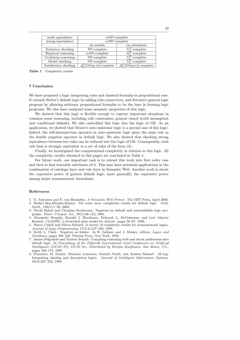
29

weak equivalence coNP-completestrong equivalence coNP-complete

− on models on extensions

Existence checking NP-complete ΣP2 -complete

Skeptical reasoning coNP-complete ΠP2 -complete

Credulous reasoning NP-complete ΣP2 -complete

Model checking NP-complete ΣP2 -complete

Satisfaction checking ∆P2 [O(log n)]-complete ∆P

2 [O(log n)]-complete

Table 1 Complexity results

7 Conclusion

We have proposed a logic integrating rules and classical formulas in propositional case.

It extends Reiter’s default logic by adding rule connectives, and Ferraris’s general logic

program by allowing arbitrary propositional formulas to be the base in forming logic

programs. We also have analyzed some semantic properties of this logic.

We showed that this logic is flexible enough to capture important situations in

common sense reasoning, including rule constraints, general closed world assumption

and conditional defaults. We also embedded this logic into the logic of GK. As an

application, we showed that Moore’s auto-epistemic logic is a special case of this logic.

Indeed, the self-introspection operator in auto-epistemic logic plays the same role as

the double negation operator in default logic. We also showed that checking strong

equivalence between two rules can be reduced into the logic of GK. Consequently, each

rule base is strongly equivalent to a set of rules of the form (3).

Finally, we investigated the computational complexity in relation to this logic. All

the complexity results obtained in this paper are concluded in Table 1.

For future work, one important task is to extend this work into first order case

and then to find tractable subclasses of it. This may have potential applications in the

combination of ontology layer and rule layer in Semantic Web. Another work is about

the expressive power of general default logic, more generally, the expressive power

among major nonmonotonic formalisms.

References

1. G. Antoniou and F. van Harmelen. A Semantic Web Primer. The MIT Press, April 2004.2. Rachel Ben-Eliyahu-Zohary. Yet some more complexity results for default logic. Artif.

Intell., 139(1):1–20, 2002.3. Nicole Bidoit and Christine Froidevaux. Negation by default and unstratifiable logic pro-

grams. Theor. Comput. Sci., 78(1):86–112, 1991.4. Alexander Borgida, Ronald J. Brachman, Deborah L. McGuinness, and Lori Alperin

Resnick. CLASSIC: a structural data model for objects. pages 58–67, 1989.5. Marco Cadoli and Marco Schaerf. A survey of complexity results for nonmonotonic logics.

Journal of Logic Programming, 17(2-4):127–160, 1993.6. Keith L. Clark. Negation as failure. In H. Gallaire and J. Minker, editors, Logics and

Databases, pages 293–322. Plenum Press, New York, 1978.7. James Delgrande and Torsten Schaub. Compiling reasoning with and about preferences into

default logic. In Proceedings of the Fifteenth International Joint Conference on ArtificialIntelligence (IJCAI–97), IJCAI Inc. Distributed by Morgan Kaufmann, San Mateo, CA.,pages 168–174, 1997.

8. Francesco M. Donini, Maurizio Lenzerini, Daniele Nardi, and Andrea Schaerf. AL-log:Integrating datalog and description logics. Journal of Intelligent Information Systems,10(3):227–252, 1998.

30

9. Thomas Eiter and Georg Gottlob. Complexity results for disjunctive logic programmingand application to nonmonotonic logics. In International Logic Programming Symposium,pages 266–278, 1993.

10. Thomas Eiter and Georg Gottlob. The complexity class theta2p: Recent results and appli-cations in ai and modal logic. In FCT ’97: Proceedings of the 11th International Symposiumon Fundamentals of Computation Theory, pages 1–18, London, UK, 1997. Springer-Verlag.

11. Thomas Eiter, Michael Fink, Hans Tompits, and Stefan Woltran. Simplifying logic pro-grams under uniform and strong equivalence. In LPNMR, pages 87–99, 2004.

12. Paolo Ferraris. Answer sets for propositional theories. In LPNMR, pages 119–131, 2005.13. Paolo Ferraris. On modular translations and strong equivalence. In LPNMR, pages 79–91,

2005.14. Michael Gelfond and Vladimir Lifschitz. The stable model semantics for logic program-

ming. In Proc. Fifth International Conference and Symposium on Logic Programming, pages1070–1080, 1988.

15. Michael Gelfond and Vladimir Lifschitz. Classical negation in logic programs and disjunc-tive databases. New Generation Computing, 9:365–385, 1991.

16. Michael Gelfond, Vladimir Lifschitz, Halina Przymusinska, and Miroslow Truszczynski.Disjunctive Defaults. In J. Allen, R. Fikes, and B. Sandewall, editors, Proceedings of thesecond Conference on Principles of Knowledge Representation and Reasoning, Cambridge,Massachusetts. Morgan Kaufmann, 1991.

17. Michael Gelfond. Logic programming and reasoning with incomplete information. Ann.Math. Artif. Intell., 12(1-2):89–116, 1994.

18. Georg Gottlob. Complexity results for nonmonotonic logics. J. Log. Comput., 2(3):397–425, 1992.

19. Georg Gottlob. NP trees and Carnap’s modal logic. Journal of the ACM, 42(2):421–457,1995.

20. Georg Gottlob. Translating default logic into standard autoepistemic logic. J. ACM,42(4):711–740, 1995.

21. B. Grosof, I. Horrocks, R. Volz, and S. Decker. Description logic programs: Combininglogic programs with description logic, 2003.

22. Joseph Y. Halpern and Yoram Moses. A guide to completeness and complexity for modallogics of knowledge and belief. Artif. Intell., 54(3):319–379, 1992.

23. Ian Horrocks and Peter F. Patel-Schneider. A proposal for an owl rules language. InWWW, pages 723–731, 2004.

24. T. Imielinski. Results on translating defaults to circumscription. Artif. Intell., 32(1):131–146, 1987.

25. Tomi Janhunen. On the intertranslatability of autoepistemic, default and priority logics,and parallel circumscription. Lecture Notes in Computer Science, 1489:216–??, 1998.

26. Kurt Konolige. On the relation between default and autoepistemic logic. Artif. Intell.,35(3):343–382, 1988.

27. Richard E. Ladner. The computational complexity of provability in systems of modalpropositional logic. SIAM J. Comput., 6(3):467–480, 1977.

28. Paolo Liberatore and Marco Schaerf. The complexity of model checking for propositionaldefault logics. Data Knowl. Eng., 55(2):189–202, 2005.

29. Vladimir Lifschitz, Lappoon R. Tang, and Hudson Turner. Nested expressions in logicprograms. Annals of Mathematics and Artificial Intelligence, 25(3-4):369–389, 1999.

30. V. Lifschitz, D. Pearce, and A. Valverde. Strongly equivalent logic programs. ACMTransactions on Computational Logic, 2(4):526–541, 2001.

31. Fangzhen Lin and Yin Chen. Discovering classes of strongly equivalent logic programs.In Proceedings of the Nineteenth International Joint Conference on Artificial Intelligence(IJCAI–05), 2005. To appear.

32. Fangzhen Lin and Yoav Shoham. A logic of knowledge and justified assumptions. ArtificialIntelligence, 57:271–289, 1992.

33. Fangzhen Lin and Yi Zhou. From answer set logic programming to circumscription vialogic of gk. In Proceedings of the IJCAI’07, 2007.

34. Wiktor W. Marek and M. Trusczynski. Nonmonotonic Logic: Context-Dependent Reason-ing. Springer-Verlag New York, Inc., Secaucus, NJ, USA, 1997.

35. V. Wiktor Marek and Miroslaw Truszczynski. Autoepistemic logic. J. ACM, 38(3):588–619, 1991.

36. R. Moore. Possible-world semantics for autoepistemic logic. pages 137–142, 1987.

31

37. Ilkka Niemela. Towards automatic autoepistemic reasoning. In JELIA ’90: Proceedings ofthe European Workshop on Logics in AI, pages 428–443, London, UK, 1991. Springer-Verlag.

38. Ilkka Niemela. A unifying framework for nonmonotonic reasoning. In ECAI, pages 334–338, 1992.

39. C. H. Papadimitriou. Computational Complexity. Addison-Wesley, Reading, MA, 1994.40. David Pearce, Hans Tompits, and Stefan Woltran. Encodings for equilibrium logic and

logic programs with nested expressions. In EPIA ’01: Proceedings of the10th PortugueseConference on Artificial Intelligence on Progress in Artificial Intelligence, Knowledge Ex-traction, Multi-agent Systems, Logic Programming and Constraint Solving, pages 306–320,London, UK, 2001. Springer-Verlag.

41. David Pearce. Equilibrium logic: an extension of answer set programming for non-monotonic reasoning. In Proccedings of WLP2000, page 17, 2000.

42. Raymond Reiter. A logic for default reasoning. Artificial Intelligence, 13:81–132, 1980.43. Riccardo Rosati. Towards expressive KR systems integrating datalog and description

logics: preliminary report. In Description Logics, 1999.44. Jonathan Stillman. The complexity of propositional default logics. In AAAI, pages 794–

799, 1992.45. Miroslaw Truszczynski. Strong and uniform equivalence of nonmonotonic theories - an

algebraic approach. In KR, pages 389–399, 2006.46. Hudson Turner. Strong equivalence for logic programs and default theories (made easy).

In LPNMR, pages 81–92, 2001.