1

5.

Radiative and Chemical Processes

5.1. Introduction

The continuity equations for reactive chemical species in the atmosphere include chemical production and loss terms determined by kinetic rate laws. Gas concentrations in the atmosphere are low, and reactions between stable species are therefore slow. A major factor driving atmospheric chemistry is solar radiation, which can photolyze otherwise stable non-radical species to produce highly reactive radicals. Radicals are chemicals with an unfilled electron orbital, i.e., an odd total number of electrons. The unpaired electron makes them highly reactive. Photolysis typically results in radical formation:

non-radical + hν → radical + radical where the non-radical molecule (even number of electrons) splits into two radicals (odd + odd). The highly reactive radical can then go on to react with a non-radical, resulting in new radical formation (odd + even):

radical + non-radical → radical + non-radical In this manner the initial photolysis event results in a radical-assisted reaction chain, with rapid transformation of non-radical species propagated by a cascade of reactions involving successive radicals. Eventually the chain is terminated by reactions between radicals (odd+odd), for example:

radical + radical → non-radical + non-radical These termination reactions tend to be slow because radical concentrations are low. Reaction chains can thus have considerable length in the atmosphere and often take the form of catalytic cycles. Because the reaction mechanisms involved in these chains are initiated by solar radiation they are often referred to as photochemical.

2

Computing the rates of photolysis reactions is a major challenge for atmospheric chemistry models and the first topic of this chapter. The rates depend on the availability of photons with sufficiently high energies (small wavelengths) to cleave the molecules. These photons are generally in the UV range of wavelengths, and their flux in the atmosphere depends in a complicated way on absorption by gases; scattering by air molecules, aerosol particles, and clouds; and reflection at the surface. The propagation of photons in the atmosphere is described by the equations of radiative transfer and we present the foundations for these equations. We go on to present the general formulations of chemical kinetics in atmospheric models. These include gas-phase reactions but also reactions involving aerosols and clouds. Aerosols and clouds occupy a minute fraction of atmospheric volume (even in a dense cloud, the liquid water content is at most a few cm3 per m3 of air). However, they enable unique chemistry to take place in the bulk condensed phase or at particle surfaces. Standard usage in atmospheric chemistry is to refer to reactions in the gas phase gas as homogeneous chemistry, and to reactions involving aerosols and clouds as heterogeneous or multiphase chemistry.

5.2. Radiative Transfer The chemical composition, thermal structure, and dynamical behavior of the atmosphere are strongly affected by the exchange of radiative energy between atmospheric layers. Electromagnetic radiation travels as a spectrum of waves of frequencies ν [Hz] or wavelengths λ [m]. Frequency ν and wavelength λ are related by

λν = c where c = 3108 m s-1 represents the speed of the light in the vacuum. Equivalently, light can be represented by a distribution of particles called photons with energy hν [J]. Here h is the Planck’s constant (6.6210-34 J s). The intensity of radiation that travels through the atmosphere is affected by emission, absorption, and scattering processes. In this Section, we present the definition of the key physical quantities that are commonly used in the theory of radiative transfer. After stating the fundamental laws that govern blackbody radiation, we present methods used to calculate atmospheric absorption and scattering of ultraviolet and visible (solar) radiation, and atmospheric emission and absorption of infrared (terrestrial) radiation. In this Chapter, the spectral distribution of a physical quantity (e.g., of the radiative flux F) is generally referred to as the spectral density of this quantity or its monochromatic value. It is expressed by the derivative versus wavelength (Fλ = dF/dλ) or versus frequency (Fν = dF/dν) of the quantity (here the flux). It is common practice in the spectroscopy literature to express radiative parameters as a function of wavelengths in the ultraviolet and visible regions of the spectrum, and as a function of frequencies or of wavenumbers (1/λ) in the infrared region. For consistency and clarity in the presentation, we will express the spectral parameters and the radiative

3

transfer equations as a function of wavelength. Expressing these quantities or these equations as a function of frequency or wavenumber is straightforward.

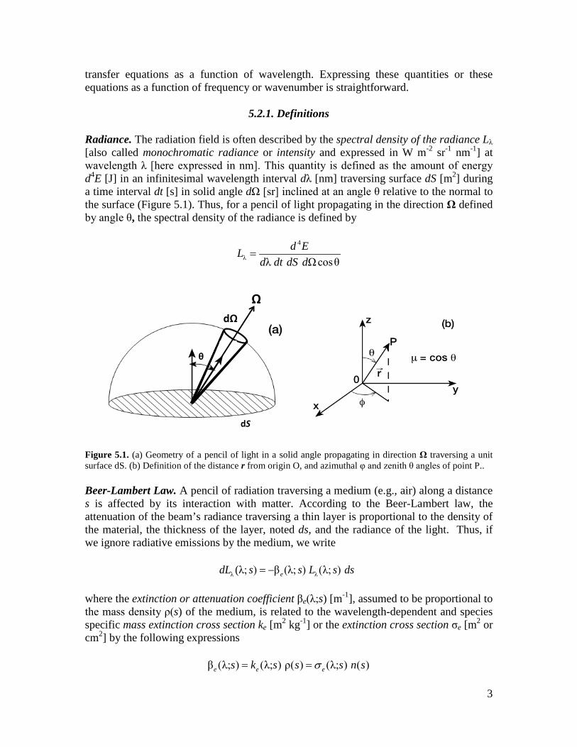
5.2.1. Definitions Radiance. The radiation field is often described by the spectral density of the radiance Lλ [also called monochromatic radiance or intensity and expressed in W m-2 sr-1 nm-1] at wavelength λ [here expressed in nm]. This quantity is defined as the amount of energy d4E [J] in an infinitesimal wavelength interval dλ [nm] traversing surface dS [m2] during a time interval dt [s] in solid angle dΩ [sr] inclined at an angle θ relative to the normal to the surface (Figure 5.1). Thus, for a pencil of light propagating in the direction Ω defined by angle θ, the spectral density of the radiance is defined by

4

λ λ Ω cosθd EL

d dt dS d=

dΩθ

dS

ΩdΩ

Figure 5.1. (a) Geometry of a pencil of light in a solid angle propagating in direction Ω traversing a unit surface dS. (b) Definition of the distance r from origin O, and azimuthal φ and zenith θ angles of point P.. Beer-Lambert Law. A pencil of radiation traversing a medium (e.g., air) along a distance s is affected by its interaction with matter. According to the Beer-Lambert law, the attenuation of the beam’s radiance traversing a thin layer is proportional to the density of the material, the thickness of the layer, noted ds, and the radiance of the light. Thus, if we ignore radiative emissions by the medium, we write

λ λ(λ; ) β (λ; ) (λ; ) edL s s L s ds= − where the extinction or attenuation coefficient βe(λ;s) [m-1], assumed to be proportional to the mass density ρ(s) of the medium, is related to the wavelength-dependent and species specific mass extinction cross section ke [m2 kg-1] or the extinction cross section σe [m2 or cm2] by the following expressions

β (λ; ) (λ; ) ρ( ) (λ; ) ( )e e es k s s s n sσ= =

4

where n [molec m-3 or molec cm-3] is the number density of molecules that interact with the light beam. The cross sections are often temperature-dependent and hence vary somewhat along the optical path. The integration of expression (5.X) yields

0

λ λ 0(λ; ) (λ; ) exp β (λ; ) s

es

L s L s s ds

= − ∫

The optical depth at wavelength λ between geometrical points s0 and s is given by

0

0τ(λ; , ) β (λ; ) s

es

s s s ds= ∫

and the corresponding transmission function T is

[ ]0 0(λ; , ) exp τ(λ; , )s s s s= −T In standard atmospheric chemistry usage (and in this chapter), the optical depth τe is defined as the extinction in the vertical direction and is then expressed as

τ ( ) β (λ; ) e ez

z z dz∞

= ∫

The extinction along an inclined direction is then referred to as the slant optical depth or optical path. Extinction includes processes of absorption (conversion of radiance to other forms of energy, such as heat) and scattering (change in the direction of the incident radiation). The extinction coefficients and optical depths are therefore often separated into absorption (a) and scattering (s) components:

βe = βa + βs, and

τe = τa + τs, The ratio between the scattering and extinction cross section is called the single scattering albedo ω(λ) :

β (λ) β (λ)ω(λ) = β (λ) β (λ) β (λ)

s s

e s a

=+

5

Radiative transfer equation. In addition to being attenuated by its interaction with matter, the energy of a pencil of light can be strengthened as a result of local radiative emission by the material or of through scattering of radiation from all directions into that pencil of light. These two processes lead to an increase in the local radiance expressed as

λ (λ; ) (λ; ) dL s j s ds= where j(λ,s) is a radiative source term that can again be assumed proportional to the density of material (j(λ,s) ~ βe(λ;s)). Combining all processes involved and defining the source function as J(λ,s) = j(λ,s) / βe(λ,s), we obtain a simple form of the radiative transfer equation

λλ

(λ; ) (λ; ) (λ; )β (λ; ) e

dL s L s J ss ds

= − +

A general expression for the radiative equation in a three-dimensional inhomogeneous atmospheric medium is provided by (Liou, 2002)

( ) λ λ1 • (λ; , ) (λ; , ) (λ; , )

β ( )e

L L J∇ = − +Ω r Ω r Ω r Ωr

where Lλ(λ, r, Ω) and J (λ, r, Ω) represent respectively the monochromatic radiance and source function in the direction defined by vector Ω (see Figure 5.1) and at spatial location point defined by vector r. In many applications, it can be assumed that radiative quantities and atmospheric parameters vary only with altitude (plane-stratified atmosphere). In this case, if the vertical optical depth rather than the geometric altitude is adopted as independent variable (dτ = –βe dz = βe cosθ ds), the radiative transfer equation takes the form

λλ

(λ; τ;μ,φ)μ (λ; τ;μ,φ) (λ; τ;μ,φ) τ

dL L Jd

= − +

where μ = cosθ. The first term on the right-hand side of this equation accounts for the attenuation of light (Beer-Lambert law), while, in the second term, the function J represents a radiative source term (local emission or light scattered from other directions). The radiance [W m-2 sr-1] at a point r of the atmosphere and for a direction Ω is given by the spectral integration of Lλ

λ0

( ) (λ; ) λL L d∞

= ∫r, Ω r, Ω

6

The spectral density of the irradiance Fλ(λ; r) [W m-2 nm-1] (also called monochromatic irradiance) at point r is defined as the energy density traversing a surface of unit area perpendicular to direction Ω integrated over all directions Ω’ of the incoming pencils of light. It is thus provided by the integration over all directions of the normal component of the monochromatic radiance

λ λ4(λ; , ) (λ; , ) cos( , ') 'F L d

π= ∫rΩ r Ω' Ω Ω Ω

This quantity is used to describe the exchanges of radiative energy in the atmosphere and hence to quantify its thermal budget. In a plane-stratified atmosphere (with an horizontal surface as the reference), the spectral density of the irradiance is calculated as a function of altitude z by the expression

2 1

λ λ0 1

(λ; ) φ μ (λ; ;μ,φ) μF z d L z dπ

−

= ∫ ∫

in which z is the altitude, φ is the azimuthal angle, and μ = cos θ where θ is the zenith angle (Figure 5.1). One often defines the upward and downward fluxes, Fλ(λ; z) and Fλ(λ; z) as

2 0

λ λ0 1

(λ; ) φ μ (λ; ;μ,φ) μ (μ > 0)F z d L z dπ

−

↑ = ∫ ∫

2 1

λ λ0 0

(λ; ) φ μ (λ; ;μ,φ) μ (μ < 0)F z d L z dπ

↓ = − ∫ ∫

with the net irradiance density being F(λ; z) = F(λ; z) – F(λ; z). The irradiance [W m-2] is obtained by integrating Fλ over the entire electromagnetic spectrum

λ0

( ) (λ, ) λF z F z d∞

= ∫

The diabatic heating Q (expressed in W m-3) resulting from the absorption of radiation (radiative energy absorbed and converted into thermal energy) is provided by the divergence of the irradiance

( )Q F= −∇r In a plane-parallel atmosphere, the diabatic heating Q(z), now expressed in K s-1 (or in K/day), is proportional to the variation of the flux F(z) with altitude z

7

1 ( )( ) ρ p

dF zQ zc dz

= −

In models using isobaric coordinates, the heating rate Q(p) is expressed as a function of atmospheric pressure p by

( )( ) p

g dF pQ pc dp

=

Here cp [J K-1 kg-1] is the specific heat at constant pressure and ρ [kg m-3] the air density, and g the gravitational acceleration. The spectral density of the actinic flux Φλ(r) at point r [expressed here in W m-2 nm-1] is obtained by integration of the monochromatic radiance over all solid angles

λ λ4(λ; ) (λ; , ) ΩL d

πΦ = ∫r rΩ

The photolysis of atmospheric molecules occurs regardless of the direction of the incident photon and is therefore dependent on the actinic flux rather than the irradiance. In the case of a plane stratified atmosphere, the spectral density of the actinic flux at altitude z is calculated by integration over all zenithal and azimuthal directions μ and φ

2 1

λ λ0 1

(λ; ) φ (λ; ;μ,φ) μz d L z dπ

−

Φ = ∫ ∫

In practical applications, the actinic flux density is often expressed relative to the number of photons (or quanta) qλ(λ; z) [photons m-2 s-1 nm-1]

λ λλ

(λ; ) (λ; )λ(λ; )ν

z zq zh hc

Φ Φ= =

where ν = c/λ is the radiation frequency and c = 3 108 m s-1 is the speed of light. At altitude z, the actinic flux q(Δλ, z) for a wavelength interval Δλ [photons m-2 s-1] is obtained by spectral integration of the spectral density qλ over this interval

λλ(λ; ) (λ; ) λq z q z d

∆∆ = ∫

To calculate photolysis frequencies of atmospheric molecules, models use spectrally integrated actinic fluxes with wavelength intervals typically in the range 1-10 nm.

5.2.2 Blackbody radiation

8

A blackbody is an idealized physical body that absorbs all incident electromagnetic radiation. All blackbodies at a given temperature emit thermal radiation with the same spectrum. The laws of blackbody emission are fundamental for understanding radiative transfer in the atmosphere. Planck’s Law: The Planck’s law describes the spectral distribution of the radiative emission for a blackbody at temperature T [K] under thermodynamic equilibrium. It assumes that photons are distributed with frequency ν according to Boltzmann statistics. Under these conditions, the spectral density Bν [W m-2 Hz-1] of the blackbody radiative emission flux is given by

3

ν 2ν

2ν 1(ν, )1h kT

hB Tc e

=−

where k is the Boltzmann constant (1.3810-28 J K-1). By using relation (5.X) between frequency and wavelength, one can also define the spectral density Bλ [W m-2 nm-1] as a function of wavelength:

2

λ 5λ

2 1(λ, )λ 1hc kT

hcB Te

=−

Stephan-Boltzmann Law: Integration of the radiant energy Bλ over all wavelengths (or of Bν over all frequencies) yields the Stefan-Boltzmann law

24

λ 5λ0 0

2 1( ) (λ, ) λ λ σλ 1hc kT

hcB T B T d d Te

∞ ∞

= = =−∫ ∫

which states that the total radiation flux B(T) [W m-2] emitted by a blackbody varies with the fourth power of its absolute temperature. Here σ = 2π5 k4/(15 c2h3) = 5.6710-8 Wm-2 K-4 is the Stefan constant. Wien’s Displacement Law: By differentiating Bλ(λ,T) with respect to λ, we find that the maximum wavelength of emission λmax is inversely proportional to the blackbody temperature:

λ 2897 μmaxT K m= The solar flux (T = 5800 K) is maximum in the visible (approximately 500 nm), while, the emission spectrum of the Earth peaks in the infrared (approximately 10 μm). See Figure 5.2.

9

Figure 5.2. Comparison between blackbody spectra representing the radiative flux emitted by the Sun (yellow) and by the Earth (red). The overlap of these two spectra is limited, so that solar and terrestrial radiation in the atmosphere can be treated separately. Source: http://scienceofdoom.com Kirchhoff’s Law: Under thermodynamic equilibrium, the emissivity of a medium at a given wavelength (defined as the ratio of the monochromatic emitting intensity to the value provided by the Planck function) is equal to the absorptivity (defined as the ratio of monochromatic absorbed intensity to the value of the Planck function). In the case of a blackbody, the values of the emissivity and absorptivity are equal to one.

5.2.3. Extra-terresrial solar spectrum The spectrum of radiation emitted by the Sun can be approximated as that of a black body at a temperature T = 5800 K. The spectral density of the solar flux [W m-2 nm-1] traversing a surface perpendicular to the direction of the solar beam at the top of the Earth’s atmosphere can then be expressed by

,λ λ(λ, ) β (λ, )RT B T∞Φ = where the dilution factor

2

β SunR

Rd

=

accounts for the distance between the Sun and the Earth (d = 1.471108 km at the perihelion and 1.521108 km at the aphelion) and for the solar radius RSun (6.96105 km). The total solar flux at the top of the Earth’s atmosphere, given by the Stefan-Boltzmann law

4( ) β σ RT T∞Φ = is equal to 1380 W m-2 for T = 5800 K, and is called the solar constant.

10

The observed solar spectrum deviates from the theoretical back-body curve because it includes contributions from different solar layers at different temperatures. The extra-terrestrial (top of the atmosphere) spectral density of the solar flux is shown in Figure 5.3. Also shown is the spectral irradiance at the surface, which is weaker than at the top of the atmosphere because of atmospheric scattering and absorption. Absorption by ozone, water vapor, and CO2 are responsible for well-defined bands where the radiation at the surface is strongly depleted. A more detailed solar spectrum in the UV region (λ < 400 nm), where sufficient energy is available to dissociate molecules and initiate photochemistry, is shown in Figure 5.4. Radiation in that region of the spectrum interacts strongly with the Earth’s atmosphere through absorption by molecular oxygen and ozone, and through scattering by air molecules. For wavelengths shorter than 300 nm, the radiation reaching the Earth’s surface is orders of magnitude lower than that at the top of the atmosphere.

Figure 5.3. Left: Spectral density of the solar irradiance spectrum at the top of the atmosphere and at sea level over the range 250 to 2500 nm. A blackbody spectrum is shown (thin black line) for comparison. Absorption features by several radiatively active gases are indicated.

11

Figure 5.4. Solar irradiance spectrum between 119 and 420 nm measured on March 29, 1992 by the SUSIM and SOLSTICE space-borne spectrometers on board the Upper Atmosphere Research Satellite (UARS). The irradiance is defined as the flux of radiative energy across a surface perpendicular to the direction of the Sun. The Lyman-alpha line at 121 nm represents solar emission by H atoms. Absorption lines produced by the singly ionized Mg and Ca atoms in the solar atmosphere are also visible. From Woods et al. (1996).

5.2.4. Penetration of Solar radiation in the Atmosphere To represent the evolution of the radiance and the radiative flux as solar radiation penetrates into the atmosphere, one has to account for atmospheric absorption and scattering by atmospheric molecules, aerosol particles and clouds as well as reflection of radiative energy by the Earth’s surface (albedo). Absorption only. Before addressing the full problem of radiative transfer for solar radiation in the atmosphere, we first consider the simple case in which absorption processes play the dominant role, with scattering assumed to be negligible. This assumption is often adopted to calculate the solar flux in the middle and upper atmosphere, where scattering is weak. The direct incoming solar beam then represents the dominant component of solar radiation and the actinic flux density qλ(λ;z,θ0) at altitude z and for a given solar zenith angle θ0 is proportional to the radiance associated with the direct solar beam. From the Beer-Lambert law, one derives

12

[ ]

λ 0 λ,

λ, 0

λ, 0

(λ; ,θ ) (λ) exp σ (λ) ( )

(λ) exp ( ,θ ) σ (λ) ( )

(λ) exp ( ,θ ) τ (λ; )

as

az

a

q z q n s ds

q z n z dz

q z z

∞

∞

∞

∞

∞

= −

= −

= −

∫

∫F

F

where qλ,¥(λ) is the spectral density of the solar actinic flux at the top of the atmosphere. The factor under the exponential describes the absorption of the solar beam by an absorber whose number density is n and wavelength-dependent absorption cross section is σa. The air mass factor F(z, θ0), defined as the ratio of the slant column density to the vertical column density,

0

( ) ( ,θ )

( )

s

z

n s dsz

n z dz

∞

∞=∫

∫F

accounts for the influence of the solar inclination. Here, n(s) represents the number density of the absorber along the light path s and n(z) the concentration of the absorber along the vertical. Note that, theoretically, the air mass factor at a given wavelength is altitude-dependent and different for different absorbers. However, if one neglects the effect of the Earth’s curvature (and assume a plane parallel atmosphere), it can be approximated for all absorbing compounds by a single function of the solar zenith angle that is independent of the altitude

0 0( ,θ ) sec θz =F In this case, ds = dz/μ0 where μ0 = cos θ0. This approximation is generally acceptable if the solar zenith angle θ0 is less than 75 degrees. Otherwise, a more complex approach must be adopted to account for the Earth’s sphericity, and F(z, θ0) can be expressed, for example, by the Chapman function (see Smith and Smith, 1972 and Brasseur and Solomon, 2005 for more details). In expression (5.X), τa(λ; z) represents the optical depth along the vertical resulting from the absorption of solar radiation from the top of the atmosphere to altitude z. Its calculation requires that the vertically integrated concentration of the absorbers (also called the vertical column) and the absorption cross section be accurately known. When several absorbers i are contributing to the attenuation of radiation, the total optical depth is the sum of the optical depth associated with the individual species:

,τ (λ; ) τ (λ; )a a ii

z z=∑

13

In the middle and upper atmosphere, the atmospheric optical depth is due primarily to the absorption by ozone and molecular oxygen, so that

,O3 ,O2τ (λ; ) τ (λ; ) τ (λ; )a a az z z= + The spectral distribution of the absorption cross sections for O2 and O3 are shown in Figures 5.5 and 5.6. Spectral regions of importance are listed in Table 5.1.

Figure 5.5. Absorption cross-section [cm2] of molecular oxygen between 50 and 250 nm featuring the Schumann-Runge continuum (130-170 nm), the Schumann-Runge bands (175-205 nm), and the Herzberg continuum (200-242 nm). Note the weak absorption cross section at the wavelength corresponding to the intense solar Lyman-α line. At wavelengths shorter of 102.6 nm, absorption of radiation leads to photo-ionization of O2.

Wavelength (nm)

O3

Abs

orpt

ion

cros

s se

ctio

n (c

m2 )

Figure 5.6. Absorption cross section [cm-2] of ozone between 180 and 750 nm with the Hartley band (200-310 nm), the temperature-dependent Huggins bands (310-400 nm) and the weak Chappuis bands (beyond 400 nm)

14

Table 5.1. Spectral Regions of Photochemical Importance in the Atmosphere Wavelength Atmospheric Absorbers 121.6 nm Solar Lyman a line, absorbed by O2 in the mesosphere. No

absorption by O3. 130-175 nm O2 Schumann-Runge continuum. Absorption by O2 in the

thermosphere. 175-205 nm O2 Schumann-Runge bands. Absorption by O2 in the mesosphere

and upper stratosphere. Effect of O3 can be neglected in the mesosphere, but is important in the stratosphere.

200-242 nm O2 Herzberg continuum. Absorption of O2 in the stratosphere and weak absorption in the mesosphere. Absorption by the O3 Hartley band is also important (see below).

200-310 nm O3 Hartley band. Absorption by O3 in the stratosphere leading to the formation of the O(1D) atom.

310-400 nm O3 Huggins bands. Absorption by O3 in the stratosphere and troposphere leads to the formation of the O(3P) atom.

400-850 nm O3 Chappuis bands. Weak absorption by O3 in the troposphere induces photodissociation all the way to the surface.

Absorption and Scattering. In addition to being absorbed by atmospheric matter, radiation is scattered by air molecules and particles. The theory of Lorenz (1890) and Mie (1908) describes the interaction between a plane electromagnetic wave and a dielectric spherical particle, and is based on the Maxwell equations. Air molecules and water droplets in low and medium clouds can be treated as spherical particles, so that the Lorenz-Mie theory applies. This is not the case, however, for solid particles including cirrus cloud particles (i.e., ice crystals). These can, however, be treated as “equivalent spheres”. Despite the simple geometry involved, the derivation of the solution for the Maxwell equations is remarkably complex, and cannot be reproduced here. Only asymptotic cases will be briefly considered. For example, the theory of Rayleigh (1871) refers to the scattering of light by particles whose size is considerably smaller than the radiation wavelength. To discuss the properties of scattered light in the atmosphere, we introduce several parameters including (1) the size parameter

πα

λpD

=

that measures the dimension of the molecule or particle (diameter Dp) relative to the wavelength λ of the incoming radiation, and largely determines the scattering regime (Figure 5.7); (2) the scattering angles that reduce to a single angle Θ when the scattering object is a sphere, and light is therefore scattered symmetrically around the incident

15

beam; (3) the refraction index m defined as the ratio of the velocity of light in vacuum to that in the air with

m = mr + i mi The real and imaginary parts of the refractive index, mr and m,, are both wavelength dependent and refer respectively to the phase speed of the light and the amount of absorption through the medium. In the pure scattering case, the refraction index is a real quantity. Scattering is affected by the degree of polarization of the light. Light emitted by the Sun is unpolarized, but becomes partially polarized after scattering with molecules and particles in the atmosphere.

Figure 5.7. Different scattering regimes as a function of radiation wavelength and particle radius. (Reproduced from G. W. Petty, 2006) Scattering by air molecules. Scattering of light by air molecules is described by the Rayleigh theory which can be viewed as asymptotic case of the Lorenz-Mie theory for a size parameter α << 1. Under these assumptions, the scattering cross section [m2] is found to be

23

4

132π(λ) (δ)3λ

rs

a

m fn

σ −

=

where na is the air number density and mr the real part of the refractive index of air. The dominant feature in this equation is the λ-4 dependence of the scattering cross section. Note that, to a good approximation, factor mr – 1 is proportional to the air density na, so that, for practical purposes, the value of σs is only dependent on the wavelength of the

16

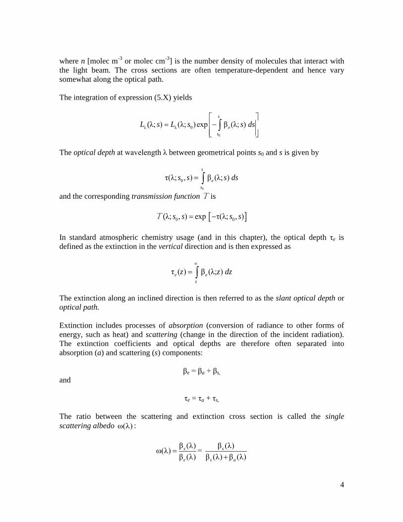
light. The correction factor f(δ) = (6 + 3δ)/(6 – 7δ) in expression (7.X) accounts for the anisotropy of non-spherical molecules with the anisotropy factor being δ = 0.035 (Liou, 2002). Scattering by aerosols and cloud droplets. Scattering due to very large particles such as cloud droplets (α >> 1) is described by the laws of geometric optics, which can be regarded as another asymptotic approximation of the electromagnetic theory. In this formulation, the direction of propagation of light rays is modified by local reflection and refraction processes. Refraction at the interface of the two media (e.g., air and water) is described by Snell Law and is a function of the refractive index of a medium versus the other. The case of smaller aerosol particles is more complex as particle dimensions are typically of the same order of magnitude as UV radiation (α ~ 1). The Lorenz-Mie theory applied to spherical aerosol particles with diameter Dp provides analytic expressions for the scattering and absorption efficiencies

2

4π

ss

p

QDσ

= and 2

4π

aa

p

QDσ

=

defined as the ratio of the scattering (σs) and absorption (σa) cross sections, respectively to the geometric section πDp

2/4, as a function of size parameter α. The extinction efficiency Qe is then defined as

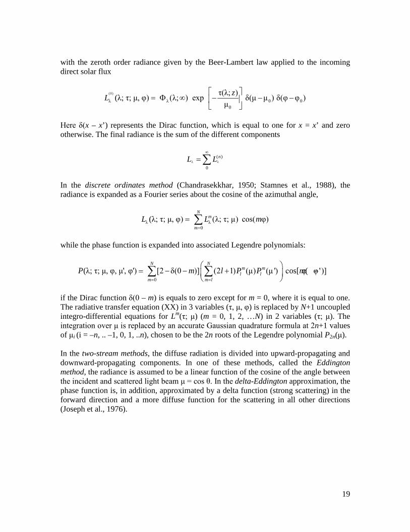
Qe = Qs + Qa Values of Qs and Qa are presented in Figure 5.8. Scattering is most efficient when the particle radius is equal to the wavelength of incident radiation (α = 2π). Scattering is inefficient for very small particles (α << 1). For very large particles (α >> 1), Qs approaches a diffraction limit. The absorption (βa) and scattering (βs) coefficients for polydisperse aerosols are obtained by integration of the respective cross sections over the size distribution of the particles.

Qs

Size Parameter α

Qa

Size Parameter α

17

Figure 5.8. Scattering (left) and absorption (right) efficiencies as a function of the aerosol size parameter α for various amounts of absorption (imaginary part of the refraction index m). From Frank Evans, University of Colorado Source Function and Phase Function. When the effects of both absorption and scattering on the solar radiance are taken into account and local emissions are ignored, the source term J that appears in the radiative transfer equation (5.X written in the case of a plane stratified atmosphere) must account for light scattered from the direction of the direct Sun (μ0, φ0) (direct light) and from all other directions (μ’, φ’). The source term J can be expressed as

0

τ(λ; )μ

0 0λω(λ)(λ; τ; μ, φ) (λ; τ; μ, φ, μ , φ ) (λ; )4π

z

J P e−

= Φ ∞

2 1

λ0 1

ω(λ) φ' (λ; τ; μ, φ, μ', φ') (λ; τ; μ, φ) μ'4π

d P L dπ

−

+ ∫ ∫

where ω(λ) = βs/βe is again the single scattering albedo. The first term on the right-hand-side of equation (5.X) represents the single scattering of the direct solar radiation (whose irradiance at the top of the atmosphere is Φλ(λ; ∞)), and the second term accounts for multiple scattering. The phase function P(λ; τ; μ, φ, μ’, φ’) defines the probability that a photon originating from direction (μ’, φ’) is scattered in direction (μ, φ). This angular distribution of the scattered energy can be derived from theory. It varies with the value of the size parameter α and with the degree of polarization of light. For scattering of unpolarized light (e.g., solar radiation) by gas molecules, Rayleigh’s theory applies (α << 1), and the phase function can be expressed as

23( ) (1 cos )4

P Θ = + Θ

where the scattering angle Θ is related to the azimuthal and zenithal directions by

2 1 2 2 1 2cosμμ' (1 μ ) (1 μ ' ) cos(φ φ')Θ = + − − − The dimensionless phase function P(Θ) is normalized by

2π

0 0

1 φ ( )sin 14π

d P dπ

Θ Θ Θ =∫ ∫

In the case of aerosol particles (α ~ 1), the Lorenz-Mie theory applies and more complex expressions, often expressed as a function of associated Legendre polynomials, can be derived. Sample phase functions are shown in Figure 5.9. Scattering by large particles is characterized by a strong forward component.

18

Figure 5.9. Left: Schematic polar representation of light scattered by particles of different sizes. Right: Scattering phase function derived from the Lorenz-Mie theory as a function of the scattering angle Θ for different values of the particle size parameter α. In the case of Rayleigh scattering (α << 1), the same amount of light is scattered in the forward and backward directions. Mie scattering (α >1) tends to favor scattering in the forward direction, especially in the case of large particles. From deepocean.net (left) and Frank Evans, University of Colorado (right). Solution of the Radiative Transfer Equation. The formal solution of the radiative transfer equation (5.X) for the upward radiance at level corresponding to an optical depth of τ is

λ0

τ τ τ' τ τ '(λ;τ,μ,φ) (λ; τ ;μ,φ) exp (λ; τ ';μ,φ)exp (μ 0)μ μ μ

ss

dL L Jτ

λ − −

= − + − >

∫

where τs is the optical depth at the surface. For the downward radiance

λ0

τ τ τ' τ '(λ;τ,μ,φ) (λ;0;μ,φ) exp (λ; τ ';μ,φ)exp (μ < 0)μ μ μ

dL L Jτ

λ −

= − + − − − − ∫

Finally, for μ = 0, the horizontal radiance is

λ λ(λ;τ,μ=0,φ) (λ; τ,μ=0,φ)L J= Different numerical methods are available to obtain approximate solutions to the integro-differential radiative transfer equation in an absorbing and scattering atmosphere. These include, for example, iterative Gauss, successive order, discrete ordinate, two-stream, and Monte-Carlo methods. See Lenoble (1977) and Liou (2002) for more details. An example is provided by the successive order method in which the solution is obtained by solving iteratively (n = 0, 1, …)

λ

λ

( 1) 2 1λ ( 1) ( )

λ λλ 0 1

(τ ;μ,φ) ω(λ)μ (τ ;μ,φ) φ' (λ; τ; μ, φ, μ', φ') (λ; τ; μ, φ) μ 'τ 4π

nn ndL

L d P L dd

π++

−

= − + ∫ ∫

19

with the zeroth order radiance given by the Beer-Lambert law applied to the incoming direct solar flux

(0)

λ λ 0 00

τ(λ; )(λ; τ; μ, φ) (λ; ) exp δ(μ μ ) δ(φ φ )μ

zL

= Φ ∞ − − −

Here δ(x – x’) represents the Dirac function, which is equal to one for x = x’ and zero otherwise. The final radiance is the sum of the different components

λ λ( )

0

nL L∞

=∑

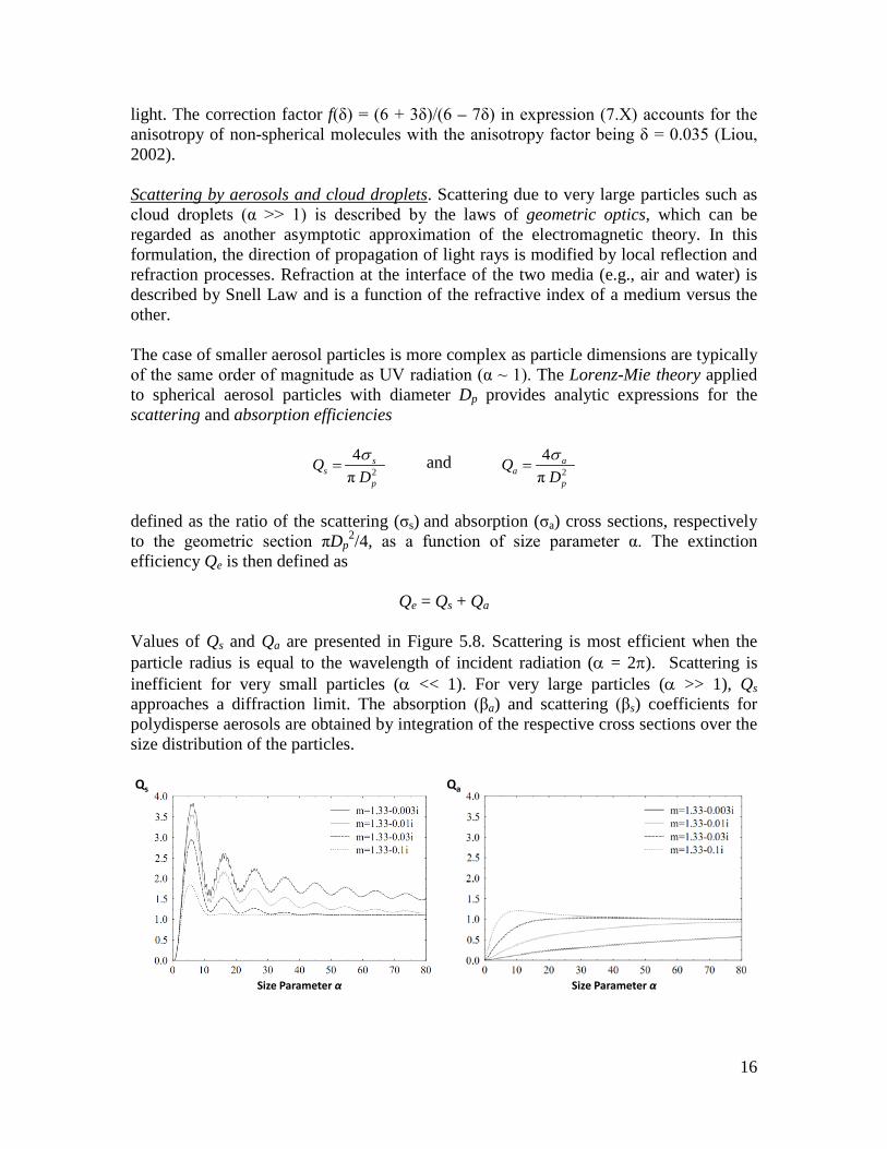
In the discrete ordinates method (Chandrasekkhar, 1950; Stamnes et al., 1988), the radiance is expanded as a Fourier series about the cosine of the azimuthal angle,

λ λ0

(λ; τ; μ, φ) (λ; τ; μ) cos( φ)N

m

mL L m

=

= ∑

while the phase function is expanded into associated Legendre polynomials:

0(λ; τ; μ, φ, μ', φ') [2 δ(0 )] (2 1) (μ) (μ ') cos[ (φ φ ')]

N Nm m

l lm m l

P m l P P m= =

= − − + −

∑ ∑

if the Dirac function δ(0 – m) is equals to zero except for m = 0, where it is equal to one. The radiative transfer equation (XX) in 3 variables (τ, μ, φ) is replaced by N+1 uncoupled integro-differential equations for Lm(τ; μ) (m = 0, 1, 2, …N) in 2 variables (τ; μ). The integration over μ is replaced by an accurate Gaussian quadrature formula at 2n+1 values of μi (i = –n, .. –1, 0, 1, ..n), chosen to be the 2n roots of the Legendre polynomial P2n(μ). In the two-stream methods, the diffuse radiation is divided into upward-propagating and downward-propagating components. In one of these methods, called the Eddington method, the radiance is assumed to be a linear function of the cosine of the angle between the incident and scattered light beam μ = cos θ. In the delta-Eddington approximation, the phase function is, in addition, approximated by a delta function (strong scattering) in the forward direction and a more diffuse function for the scattering in all other directions (Joseph et al., 1976).

20

Figure 5.10. Land surface albedo at 470 nm. Data based on MODIS observations in June 2001. Areas where no data are available are shown in grey. Image from MODIS Atmosphere support Group incl. E. Moody, NASA, GSFC and C. Schaaf, Boston University and NASA. Albedo. Radiation reflected by the surface must be included in the calculation of the radiance through a lower boundary condition of the type

λ λ(μ > 0, φ; 0) (μ < 0, φ; 0)L z L z= = =A where the surface albedo A varies with surface type (Figure 5.10), wavelength, and the incident and reflected zenith and azimuthal angles. It is frequently assumed that the albedo is isotropic (the surface is then called Lambertian) but this is often not precise enough for retrieval of atmospheric parameters such as aerosol optical depth from satellite measurements of solar backscatter. In those cases one needs to describe the full angular dependence of the surface albedo, known as the bidirectional reflectance distribution function (BRDF).

5.2.5. Emission and Absorption of Terrestrial Radiation

In the infrared, at wavelengths larger than approximately 3.5 μm, the radiation field is determined primarily by radiative emission from the Earth’s surface and the atmosphere. At these wavelengths, the contribution of the solar radiation is small, and, in addition, scattering by air molecules can be neglected. Because of the limited overlap between solar (shortwave) and terrestrial (longwave) radiation, a clear distinction can be made in the approach that is adopted to solve the radiative transfer equation. In the case of longwave radiation, the spatial distribution of the radiance is derived by integrating the radiative transfer equation (5.X) in which the source function is represented by the Planck’s function Bλ(λ,T). This formulation requires that collisions be sufficiently frequent so that the energy levels of the molecules are populated according to the Boltzmann distribution (local thermodynamic equilibrium (LTE)). This condition is met in the lower atmosphere, but LTE breaks down in the upper levels of the atmosphere (typically above 60-90 km, depending on the spectral band) where collisions become

21

infrequent (see Lopez-Puertas and Taylor, 2001 or Goody and Yung, 1995 for more details). In the limit of no scattering and for LTE conditions, radiative transfer is described by the Schwarzschild’s equation

λλ

λ

(τ; μ, φ)μ (τ; μ, φ) (λ; (τ))τ

dL L B Td

= −

Assuming azimuthal symmetry (no dependence of the radiance on angle φ), and providing the boundary conditions Lλ(λ; zsurface; μ > 0) = Bλ(λ; Ts) at the surface and Lλ(λ, ∞, μ < 0) = 0 at the top of the atmosphere, the upward and downward components of the radiance at altitude z and for the zenith direction μ are obtained by integration of (5.X)

λ λ λ0

(λ; ', ;μ)(λ; ,μ) (λ; ) (λ; ,0;μ) (λ; ') ' (μ > 0)'

z

sz zL z B T z B z dzz

∂= +

∂∫TT

and

λ λ(λ; ', ;μ)(λ; ,μ) (λ; ') ' (μ < 0)

'z

z zL z B z dzz

∞ ∂= −

∂∫T

where Ts represents the temperature at the Earth’s surface and

0

'(λ; ', ; μ) exp β (λ; ')μ

z

adzz z z

= −

∫T

the transmission function between altitudes z and z’ for an inclination μ and wavelength λ. Here, βa(λ, z) represents the absorption coefficient [m-1]. Its value is proportional to the concentration of the absorbers and to their wavelength-dependent absorption cross sections. Absorption of radiation by molecules in the IR involves transitions between vibrational and rotational energy levels of the molecule, as opposed to absorption in the UV which involves transitions between electronic levels. Vibrational transitions generally require λ < 20 µm, while rotational transitions require λ > 20 µm. Combined vibrational+rotational transitions lead to fine absorption structure. The radiation emitted by the Earth is mainly in the wavelength range λ < 20 µm, so that absorption by molecules must generally involve vibrational transitions. Molecules that absorb in that range are called greenhouse gases, since their absorption reduces the flux of terrestrial radiation escaping to space. A selection rule of quantum mechanics is that vibrational transitions are allowed only if they change the dipole moment of the molecule. All molecules with an asymmetric distribution of charge (H2O, O3, N2O, CO, chlorofluorocarbons) or the ability to acquire a distribution of charge by stretching or flexing (CO2, CH4) are greenhouse gases. Homonuclear diatomic molecules and single atoms (N2, O2, Ar) are not greenhouse gases. A particularity of the atmosphere of the Earth is that the dominant constituents are

22

not greenhouse gases. Figure 5.11 shows the atmospheric absorption of terrestrial radiation in the IR from 1 to 16 μm. The strongest bands are the 15 μm and 4.3 μm CO2 bands, the 9.6 μm ozone bands, the 6.3 μm water band, the 7.66 μm CH4 band, the 7.78 μm and 17 μm N2O bands, and the 4.67 μm CO band. The calculation of the infrared radiance by equation (5.X) requires quantitative knowledge of the absorption spectrum for the different radiatively active trace gases. Detailed radiative transfer models calculate the radiance under different conditions and derive the corresponding atmospheric heating rates. With sufficient spectral resolution, these models account for detailed spectral features, but this approach is often too cumbersome for model applications. In high resolution models, the spectral shape of each line must be specified: on top of their extremely narrow natural width determined by the uncertainty principle of quantum mechanics, the lines are broadened in the atmosphere as a result of different processes: at low pressure (high altitudes) with few collisions, the line width results from thermal motions of the molecule (pressure independent Doppler line width). At higher pressure (lower altitudes), broadening is determined by collisions between molecules. In practical applications, the full complexity of the spectra cannot be accounted for and parameterizations of the transmission function must be developed. These involve narrow or broad band models in which the transmission function over a specified spectral interval is derived by assuming a particular statistical distribution of the line positions and intensities within this interval. The correlated k-distribution method (Goody et al., 1989; Fu and Liou, 1992) is frequently used.

Figure 5.11. Vertical atmospheric transmission (absorption) of infrared radiation from the surface to the top of the atmosphere represented as a function of wavelength (1-16 μm) for different radiatively active gases. The different absorption bands and an aggregate spectrum are represented. Adapted from Shaw (1953).

23

The heating/cooling rate resulting from radiative energy exchanges between atmospheric layers is obtained by the divergence of the irradiance. Radiative transfer in the infrared leads to cooling of the stratosphere (primarily through emission of terrestrial radiation to space), and to warming of the troposphere-surface system (i.e., through the greenhouse effect).

5.3. Gas Phase Chemistry

5.3.1. Photolysis When a photon absorbed by a molecule exceeds in energy one of the chemical bonds of that molecule, it can cause cleavage of the bond and lead to two molecular fragments. This process is called photolysis, photodissociation, or photodecomposition. For example, molecular oxygen has a chemical bond between its O atoms corresponding to the energy of a 242 nm photon. It follows that only photons of stronger energy (shorter wavelength) can drive O2 photolysis:

2Oν (λ 242 ) O Oh nm+ ≤ → + The rate at which O2 is photolyzed is given by

[ ] [ ]2

2O 2

OO

dJ

dt= −

where JO2 represents the photolysis or photodissociation frequency [generally expressed in s-1]. Another example is the photolysis of ozone by photons of wavelengths less than 320 nm:

13 2Oν (λ 320 ) O( ) Oh nm D+ ≤ → +

where the oxygen atom is produced in its electronically excited state 1D rather than in the fundamental energy state 3P. Photons of weaker energy can only produce O(3P). In the general case where a molecule A is photolyzed and

[ ] [ ]A

AA

dJ

dt= −

the photodissociation frequency of A is derived through a spectral integration of the product of three quantities : the wavelength-dependent absorption cross section σA(λ), the quantum efficiency or quantum yield εA(λ) and the solar actinic flux qλ

24

maxλ

A A Aλ0

( ,χ) ε ( ) σ (λ) λJ z q dλ= ∫

where λmax is the wavelength corresponding to the energy threshold for dissociation of the molecule. The absorption cross section [cm2 molecule–1] represents the ability of a molecule to absorb a photon at a particular wavelength, and the quantum efficiency [unitless] represents the probability that this absorption will lead to photodissociation. Numerical integration of (5.X) over spectral intervals Δλ is straightforward when the absorption spectrum is a continuum. In certain cases, however, the absorption spectrum of molecules exhibits complex structures of discrete bands with a large number of narrow spectral lines. Examples of such structures are the Schumann-Runge bands (175-205 nm) of molecular oxygen and several bands of nitric oxide (e.g., the δ-bands) in the same spectral area. In this case, rather than reducing by several orders of magnitude the size of the spectral interval used in the numerical integration, parameterizations are adopted by which, for example, the absorption cross section or the transmission function are replaced by effective values that apply over rather large spectral intervals (see Box 5.1).

5.3.2. Elementary Chemical Kinetics Gas-phase chemical reactions can be classified for kinetic purposes as unimolecular, bimolecular, and termolecular (or 3-body). A unimolecular reaction involves the dissociation of a molecule by photons (photolysis) or heat (thermolysis). It has the general form

A C D (photolysis)

A C D (thermolysis)

hν+ → +

→ +

where A is the reactant and C and D are its dissociation products. The rate of reaction is given by

[A] [C] [D] [A]d d d kdt dt dt

− = = =

where k is a rate coefficient for the reaction, usually given in units of s-1. For photolysis reactions, this rate coefficient (also called photolysis frequency) is commonly denoted J (see Section 5.3.1).

25

Box 5.1. Photolysis in the Schumann-Runge Bands The Schumann-Runge bands (175-205 nm) feature high-frequency variations in the absorption cross sections of molecular oxygen (Figure 5.5).These high-frequency variations complicate the calculation of photolysis rates by numerical integration over the wavelength spectrum. Accounting for the Schumann-Runge bands is important for computing photolysis frequencies in the upper stratosphere and mesosphere. Scattering is negligible at those altitudes so that the actinic flux is defined by attenuation of the direct beam by O2 and O3. The photolysis frequency of a species A at altitude z can be calculated as:

A 0 A , 2 0 3 0( ,θ ) σ ( λ ) ( λ ) ( λ , ,θ ) ( λ , ,θ )k k k O k O kk

J z q z z∞= ∆ ∆ ∆ ∆∑ T T

where σA (Δλk) is the mean absorption cross section over the wavelength interval Δλk, qk,∞(Δλk) = ∫Δλk qλ,∞(λ) dλ is the mean top-of-atmosphere actinic flux over that interval, O2T

and O3T are the effective O2 and O3 transmission functions averaged over Δλk, and θ0 is the solar zenith angle. We have assumed a quantum yield of unity for simplicity of notation. The effective O2 transmission function O2T is defined by

λ, O2 0

O2 0λ,

(λ) (λ, ,θ ) λ(λ , ,θ )

(λ) λk

k

k

q z dz

q dλ

λ

∞∆

∞∆

∆ =∫

∫

T

T

where TO2 is the actual transmission function accounting for the fine absorption structure. For A = O2, the photodissociation coefficient is given by

O2 0 2 0 , O2 0 O3 0( ,θ ) σ ( λ , ,θ ) ( λ ) ( λ , ,θ ) ( λ , ,θ )SRBO k k k k k

kJ z z q z z∞= ∆ ∆ ∆ ∆∑ T T

where the effective O2 cross section for wavelength interval Δλk is defined as

O2λ, O2 0

O2 0λ, O2 0

σ (λ) (λ) ( λ , ,θ ) λσ ( λ , ,θ )

(λ) ( λ , ,θ ) λk

k

kSRB

kk

q z dz

q z dλ

λ

∞∆

∞∆

∆

∆ =∆

∫

∫

T

T

Rather than performing a computationally expensive line-by-line calculation of the effective parameters σO2

SRB and O2T , these parameters can be expressed by empirical formula as a function of the slant O2 column density

0 2secθ ( ) z

N n O dz∞

= ∫

(see e.g., Kockarts, 1994). Gijs et al. (1997) adopt the following expression

26

A bimolecular reaction has the general form

A B C D+ → + and the rate of reaction is given by

[A] [B] [C] [D] [A][B]d d d d kdt dt dt dt

− = − = = =

where the rate coefficient k is usually given in units of cm3 molecule-1 s-1. The reaction rate k[A][B] is proportional to the number of collisions ZAB per unit time between A and B. This collision frequency can be derived from the gas kinetics theory; it is proportional to the collision cross section π (rA + rB)2 and the thermal velocity

128 1 1

πthA B

kTvm m

= +

if r and m are the molecular radii and masses of A and B. Thus

ZAB = π (rA + rB)2 vth [A] [B]. As the reaction proceeds, an activated complex AB* is formed (transition state), which breaks down either to the original reactants A and B or to the products C and D. The minimum energy needed to form the activated complex is called the activation energy Ea [J mol-1]. Gas kinetics theory shows that the fraction of collisions with an energy larger

[ ]O2lnσ ( ) ( ) ( ) 220 ( )SRB N A N T N K B N = − +

where T(N) is the temperature [K] at the altitude where the column is equal to N. Coefficients A and B are expressed as a function of N, using Chebyshev polynomial fits. The effective transmission is then derived by noting that

( )O2

O2

( )σ ( )SRB

d NN

dN= −

T

Other methods to parameterize these effective coefficients have been developed by Fang et al (1974), Minschwaner et al. (1993), Zhu et al. (1999) and others. Minschwaner and Siskind (1993) have derived fast methods to calculate the photolysis frequency of nitric oxide using a similar approach. Chabrillat and Kockarts (1997) propose a parameterization for the calculation of photodissociation coefficients in the spectral range close to the Lyman (121 nm) where both the solar flux and the O2 absorption cross section vary rapidly over a narrow spectral interval.

27

than Ea is proportional to exp [– Ea/RT], so that the reaction rate coefficient can be written

( )12

2A B

8 1 1( ) π expπ

a

A B

EkTk T r rm m T

− = + + P

R

where P, the steric factor, accounts for the processes that are not included in the simple collision theory. This last equation provides a justification for the empirical Arrhenius equation (Figure 5.13)

( ) exp aEk T AT

− = R

Here, R is again the gas constant equal to 8.314 J mol-1 K-1 and A is the so-called pre-exponential factor. We see from equation (5.X) that A varies with the square root of the temperature T, but this weak dependence is often ignored. If the enthalpy ∆H of the reaction (difference between the enthalpy of formation of the products C and D and of the reactants A and B) is negative, the reaction is said to be exothermic and may proceed at a significant rate, depending on the stability of the reactants. Otherwise the reaction is said to be endothermic and much less likely to occur at a significant rate.

Figure 5.13. Energy transfer along a reaction path. The activation energy is the minimum amount of energy needed for colliding species to react. The heat of reaction is the potential energy difference between the reactants and products. The reaction is said to be exothermic if heat is released by the reaction. Otherwise, it is said to be endothermic, and heat must be absorbed from the environment.

A three-body reaction describes the combination of two reactants A and B to form a single product AB. It involves a combination of steps. The first step involves collision of the reactants to form a product AB* that is internally excited due to conversion of the kinetic energy of the colliding molecules:

28

1( ); A + B AB*k → The excited product AB* either decomposes

2( ); AB* A + Bk → or is thermally stabilized by collision with an inert third body M (in the atmosphere, M is mainly N2 and O2):

3( ); AB* + M AB + M*k → where the asterisk describes the addition of internal energy to M. This internal energy is eventually dissipated as heat. Thus, the overall reaction is written

A + B + M AB + M→ Although M has no net stoichometric effect in the overall reaction, it is important to include it in the notation of the reaction because it can play a kinetic role. The rate of the overall reaction is given by

3[A] [B] [AB] [AB*][M]d d d kdt dt dt

− = − = =

where [M] is effectively the air density [molecules cm-3]. AB* has a very short lifetime and is therefore lost as rapidly as it is produced; this defines a quasi steady-state (as opposed to true steady state, since the concentration of AB* is still changing with time). The corresponding steady-state expression is

( )1 2 3[A][B] [M] [AB*]k k k= + Replacing into equation (X) we obtain

1 3

2 3

[A][B][M][A] [B] [AB][M]

k kd d ddt dt dt k k

− = − = =+

which is the general rate expression for a three-body reaction. It has two limits. In the limit [M] << k2/k3 (low-pressure limit), the right-hand side of equation (X) reduces to (k1k3/k2)[A][B][M]. The rate then depends linearly on the air density. In the limit [M] >> k2/k3 (high-pressure limit), the right-hand side of (5.X) reduces to k1[A][B]. The rate is then independent of the air density, as [M] is sufficiently high to ensure that AB* reacts mainly by reaction (5.X) rather than by reaction (5.X).

5.4. Multiphase and Heterogeneous Chemistry

29

So far, we have discussed reactions involving the gas phase. The atmosphere also contains liquid and solid phases in the forms of aerosols, clouds, and precipitation. This enables a different type of chemistry. Chemical species partition between the gas and the condensed phase, and reactions can take place at the surface or in the bulk of the condensed phase (Figure 5.14). Standard usage is to refer to this chemistry as multiphase or heterogeneous. Some authors make a distinction between multiphase chemistry as involving reactions in the bulk condensed phase, and heterogeneous chemistry as involving surface reactions, but in practice these two terms are used interchangeably.

Figure 5.14. General schematic for uptake of a chemical species A by an aqueous aerosol particle with subsequent reaction to produce species B. Chemical reactions are indicated by solid arrows and molecular diffusion transport by dashed arrows. We see from Figure 5.14 that heterogeneous chemistry involves a combination of molecular diffusion, interfacial equilibrium, and chemical reaction. We examine here how these processes determine the rate of the overall reaction.

5.4.1. Gas-particle equilibrium Chemical species in the atmosphere partition between the gas and particle phases in a manner determined by their free energies in each phase. This equilibrium partitioning always holds at the gas-particle interface, and extends to the bulk gas and particle phases in the absence of mass transfer limitations (Figure 5.14). Mass transfer limitations will be discussed in section 5.4.2 In the case of liquid particles, the time scale to achieve gas-particle bulk equilibrium is typically less than a few minutes. Gas-particle equilibrium for a species X is described by

X(g) ⇌ X(a) where X(g) and X(a) denote the species in the gas and aerosol phases, respectively. The general form of the equilibrium constant is

30

[ ]X( )

x

aK

p=

where px is the partial pressure of X and [X(a)] is the concentration in the particle phase. Different specific forms and measures of concentration are commonly used depending on the type of particle phase and equilibrium parameterization. Aqueous solutions. When the particle phase is an aqueous solution (aqueous aerosol or cloud), the equilibrium expression (5.X) is called Henry’s law and K is called the Henry’s law constant. [X(a)] (commonly written [X(aq)]) is the molar concentration (or molarity) of the species in solution. In the atmospheric chemistry literature, K is commonly given in units of [M atm-1] where M denotes moles per liter of solution. The Henry’s law constant varies with temperature T [K] according to the van’t Hoff law

1 1( ) (298 K)exp ( )298

K T KT

∆ = − − H

R

where ΔH represents the enthalpy of dissolution at 298 K [J mol-1] and R = 8.314 J K-1 mol-1. ΔH is always negative for a gas-to-liquid transition so K increases with decreasing temperature. Table 5.2 lists the Henry’s law constants for selected species. Dependences on temperature are strong; a typical value ΔH/R = –5900 K implies a doubling of K for every 10 K temperature decrease.

Table 5.2. Henry’s law constants K for selected species (from Jacob, 2000)a

Species K(298K) [M atm-1] ΔH/ R [K] K* [M atm-1]

O3 1.1 (-2) -2400 1.8(-2) H2O2 8.3 (4) -7400 4.1(5) CH3OOH 3.1 (2) -5200 9.5(2) CH2O 1.7 (0) -3200 1.4(4) HCOOH 8.9 (3) -6100 2.2(5) HNO3 2.1 (5) -8700 4.3(11)

a Read 1.1(-2) as 1.1x10-2. Effective Henry’s law constants K* are calculated at T = 280 K and pH=4.5, including complexation with water for CH2O and acid dissociation for HCOOH and HNO3. Dissociation or complexation of the species in the aqueous phase can increase the apparent solubility beyond the physical solubility. Consider for example the dissociation of an acid species HA:

HA(g) ⇌ HA(aq)

HA(aq) ⇌ H+ + A–

with acid dissociation constant

31

( )

–H A

HAaKaq

+ =

To account for the dissociation of HA in the aqueous phase, we define the effective Henry’s law constant K* as

( ) –

HA

HA A* 1

[ ]a

aq KK Kp H +

+ = = +

Similar expressions can be derived for other dissociation or complexation processes. The dimensionless partitioning coefficient f of a species X between the aqueous phase and the gas phase can be defined by the concentration ratio in the two phases, referenced in both cases to the volume of air:

( )(X) ( )

x

x

n aqf L K R Tn g

= =

where L is the liquid water content (volume of liquid water per volume of air) and R is the ideal gas constant (0.0821 atm M-1 K-1). If X(aq) dissociates or complexes, K should be replaced by K*. In a typical cloud with L = 1x10-7 and with values from Table 5.2 for T = 280 K, H2O2 partitions roughly equally between the gas and cloudwater phase (f(H2O2) = 0.96), while HNO3 is ~100% in the cloudwater. The other species in Table 5.2 are mostly in the gas phase. In a typical non-cloud aerosol with L < 1x10-9, only HNO3 is partitioned into the aerosol phase and only in the presence of excess base (such as NH3) to drive acid dissociation. Non-aqueous solutions. Gas-particle equilibrium involving non-aqueous solutions is less well understood. Formation of organic aerosol is thought to involve at least in part an equilibrium partitioning between semi-volatile organic vapors and the organic phase of the aerosol:

[X( )][X( )]O

aKC g

=

where [X(g)] and [X(a)] are the gas- and particle-phase concentrations of X, and CO is the concentration of pre-existing organic aerosol, all in units of mass per volume of air, Non-linearity in gas-particle partitioning arises because condensation of X contributes to CO. An alternative way to express the same equilibrium is with respect to the volatility of the species, CX* = 1/K in units of mass per volume of air. The partitioning coefficient between the particle and the gas phases is given by f = CO/CX*, illustrating the dependence on CO. Because of the very large number of different species contributing to organic aerosol formation, an alternate method to tracking individual species is to group them into a limited number of volatility classes Ci* that are transported independently in

32

the model as their total (gas + particle) concentration Ci. Gas-particle partitioning is then diagnosed locally by

with *

OO i i i

i i

CC f C fC

= =∑

The solution to CO must be obtained iteratively. Solid particles. Equilibrium between the gas phase and solid particles is in general very poorly understood and depends on the surface area concentration A of the particles (surface area per unit volume of air) and the vapor pressure of the species adsorbed to the surface. One can write

[X( )] X

aKA p

=

and estimate K on the basis of the vapor pressure for the adsorbed species. This vapor pressure may strongly depend on the nature of the surface, which evolves in the atmosphere as a result of condensation, oxidation, etc. Thus, the equilibrium calculation is poorly constrained. A notable exception is the H2SO4-HNO3-NH3 aerosol, for which the thermodynamics of gas-particle partitioning of HNO3 and NH3 is well established even when the aerosol is dry (Martin, 2000).

5.4.2. Mass transfer limitations We now examine the mass transfer limitations to the atmospheric partitioning of molecules between the gas and condensed phases. The uptake rate of gas molecules by an aerosol can be expressed in a general form by

in

= gT g

dnk An

dt

−

where ng is the number density in the bulk gas phase, A is the aerosol surface area concentration (cm2 per cm3 of air), and kT is a mass transfer rate coefficient (cm s-1) that depends on molecular speed, the probability that collision will result in uptake, and any limitations from molecular diffusion. The rate of volatilization from the aerosol surface to the gas phase is proportional to the surface concentration ns in the aerosol phase

out

= g sT

dn nk Adt K

where K is the dimensionless equilibrium constant between the gas and the aerosol. The mass transfer rate constant kT is the same for uptake and for volatilization since the processes involved are the same. The net rate of transfer at the interface is

33

= g sT g

dn nk A ndt K

− −

and vanishes to zero at equilibrium. The form of kT depends on the Knudsen number Kn = a/ l, where a is the aerosol particle radius and l is the mean free path for molecules in the gas phase. The mean free path for air is l = 0.18 µm under standard conditions of temperature and pressure (STP; 273 K and 1 atm) and varies inversely with pressure. In the limit Kn << 1, the gas-phase concentration in the immediate vicinity of the particle is the same as in the bulk, since the particle does not interfere with the random motion of the gas molecules. This is called the free molecular regime. From the kinetic theory of gases, we then have

α 4T

vk =

where v = (8kT/πm)1/2 is the mean molecular speed, α is the mass accommodation coefficient representing the probability that a gas molecule impacting the surface is absorbed in the bulk, k is the Boltzmann constant, and m is the molecular weight. α generally increases with the solubility of the gas and decreases with temperature. It can approach unity for a highly soluble gas at low temperature but may be several orders of magnitude lower for a gas of low solubility.

Figure 5.15. Gas-phase concentration gradient in the vicinity of an aerosol particle of radius a. The mass transfer limitation takes on a different form in the limit Kn >> 1. Under those conditions, gas molecules in the immediate vicinity of the surface undergo a large number of collisions with the surface before being able to escape the influence of the surface and migrate to the bulk. Thus, the gas concentration at the interface is controlled by local equilibrium with the aerosol, and transport between the surface and the bulk gas phase is controlled by molecular diffusion. This is called the continuum regime. A steady-state concentration gradient is established between the particle surface and the bulk gas phase, in contrast to the free molecular regime where there is no such gradient

34

(Figure 5.15). Assuming a spherical aerosol, the gas-phase diffusion equation in spherical coordinates is

2 22

( )1( ) 0gg g g

dn rdD n r D rr dr dr

∇ = =

where Dg is the molecular diffusion coefficient and r is the distance from the center of the particle. Solving for the flux F at the gas-particle interface, we obtain

( )g sg g

r a

D ndnF D ndr a K=

= − = ∞ −

where ng(∞) is the bulk gas-phase concentration far away from the surface (ng in equation (5.X)). Thus, in the continuum regime,

gT

Dk

a=

Note that mass transfer in the continuum regime is not dependent on the mass accommodation coefficient α; this is because gas molecules trapped in the immediate vicinity of the surface collide many times with the surface and thus eventually become incorporated in the bulk aerosol phase even if α is low. By contrast, mass transfer in the free molecular regime is not dependent on the particle radius a because the particles are too small to affect the motion of molecules. The free molecular regime generally applies to stratospheric aerosols where a ~ 0.1 µm and l ~ 1 µm. The continuum regime generally applies to tropospheric clouds where a ~ 10 µm and l ~ 0.1 µm. Tropospheric aerosols are often in the transition regime since a ~ l ~ 0.1-1 µm. Exact solution of mass transfer for the transition regime is complicated. Schwartz (1986) showed that the solution can be approximated to within 10% by harmonic addition of the mass transfer rate coefficients for the free molecular and continuum regimes as two conductances operating in series:

14 α T

g

akD v

−

= +

Equation (5.X) can be applied in the general case to calculations of gas-aerosol mass transfer, as it tends towards the appropriate limits in the free molecular and continuum regimes. Unless in the free molecular regime, one should integrate over the aerosol size distribution in order to resolve the dependence of kT on the particle radius a. The volatilization component of the gas-aerosol transfer flux was expressed in equation (5.X) as a function of the surface concentration ns. This is not in general a known

35

quantity and we would like to relate it to the bulk aerosol phase concentration, which is more easily measured or modeled. The mixing time scale for a particle of radius a is given by 2 2 /πmix aa Dτ = , where Da is the molecular diffusion coefficient in the aerosol phase. For a liquid aqueous phase Da ~ 10-4 cm2 s-1 and thus for a particle with a ~ 1 µm we have τmix ~ 10-5 s. This is in general sufficiently short to ensure complete mixing of the aerosol phase so that the surface concentration equals the bulk concentration. There are a few exceptions where the diffusion equation needs to be solved in the aerosol phase (Jacob, 2000).

5.4.3. Reactive uptake probability Detailed treatment of heterogeneous chemistry in atmospheric models requires solution of the chemical evolution equations in the aerosol phase coupled to the gas phase through mass transfer. A simplified treatment is possible when the heterogeneous chemistry of interest can be reduced to a first-order chemical loss in the aerosol phase for a species transferred from the gas phase. Since the mass transfer processes are themselves first-order, the combined process can be encapsulated in a first-order loss equation. For this purpose, we define the reactive uptake probability γ as the probability that a molecule impacting the particle surface will undergo irreversible reaction rather than volatilization back to the gas phase. The rate of loss for the species from the gas phase can then be represented by equation (5.X) but with γ replacing α in the formulation of kT:

14γ T

g

akD v

−

= +

Figure 5.16. The reactive uptake probability convolves processes of gas-aerosol interfacial equilibrium, aerosol-phase diffusion, and reaction.

The reactive uptake probability convolves the processes of interfacial equilibrium, aerosol-phase diffusion, and reaction (Figure 5.16). It is a particularly helpful formulation because uptake rate coefficients from laboratory experiments are often reported as γ. One can relate γ to the actual chemical rate coefficient for loss in the aerosol phase. If the loss is a surface reaction, then γ simply compounds the mass accommodation α by the probability that the molecule will react on the surface (rate coefficient kS in unit of s-1) versus desorb (rate coefficient kD in unit of s-1). Thus,

36

α γ S

S D

kk k

=+

If the loss is a reaction taking place in the bulk of a liquid aerosol phase (rate coefficient kC in unit of s-1), then the effect of diffusion in the aerosol phase needs to be considered. Solution of the diffusion equation for a spherical particle with a zero-flux boundary condition at the particle center yields

1

1/2

1γα 4 ( ) ( )a C

vK D k f q

−

= +

where

1( ) coth f q qq

= −

and q = a(kC/Da)1/2 is a dimensionless number commonly called the diffuse-reactive parameter (Schwartz and Freiberg, 1981). f(q) represents a sphericity correction for the limitation of uptake by diffusion in the aerosol phase and is a monotonously increasing function of q. Limits are f(q) → q/3 for q → 0 and f(q) → 1 for q →∞.. It is important to recognize the sphericity correction when applying γ values measured in the laboratory to atmospheric aerosols, because the geometry used in the laboratory is different from that in the atmosphere. The laboratory measurements are often for a bulk liquid phase with planar surface (a →∞ ⇒ q →∞), so that the effective γ for an aerosol will be lower. Physically, this is because the small size of the aerosol particles does not allow diffusion of the dissolved gas into an infinite bulk but instead forces revolatilization to the gas phase. A proper treatment requires that one relate γ measured in the laboratory to kC, which is the fundamental variable, and then apply equation (5.X) (with integration over the aerosol size distribution) for the actual atmospheric aerosol conditions. This is generally ignored in atmospheric models under the implicit argument that uncertainties in kC trump other uncertainties, so that only order-of-magnitude estimates of γ are possible in any case; but the sphericity correction should then be recognized as a source of bias.

5.5. Chemical Mechanisms

The chemical operator of an atmospheric model solves the chemical evolution equation

ii i i

dn P ndt

= −

for the ensemble of species i of interest. Here ni is the number density [molecules cm-3], Pi is the production rate [molecules cm3 s-1] representing the sum of contributions from

37

all reactions producing i, and ℓini [molecules cm-3 s-1] is the loss rate representing the sum of contributions from all reactions consuming i. If Pi and ℓi are constants, then the solution to (5.X) is a simple exponential approach to the steady state Pi/ℓi:

( )( ) (0)exp[ ] 1 exp[ ]ii i i i

i

Pn t n t t= − + − −

The problem is far more complicated if Pi and ℓi depend on the concentrations of other species that are themselves coupled to species i. This is frequently the case in atmospheric chemistry because of catalytic cycles, reaction chains, and common dependences on oxidant concentrations. One must then solve equation (5.X) for the ensemble p of coupled species as a system of coupled ordinary differential equations (ODEs). Computational methods for this purpose are described in chapter 6. Here, we discuss the general task of defining the ensemble of coupled species and reactions that need to be taken into account in a chemical transport model to address a particular problem. This collection of reactions represents the chemical mechanism. It includes not only the species of interest to the problem but also the precursors and reactants for these species, which themselves may have precursors and reactants. The mechanism must represent a closed system where the concentrations of all species can be computed. Box 5.2 gives an example of a simple mechanism. The list of possible reactions involving atmospheric species is exceedingly large but only a small fraction is sufficiently fast to need to be taken into account. Placing limits on the size of the chemical mechanism is essential for computational tractability of the model. The computational cost is mainly driven by the number p of coupled species and the stiffness of the system. If a species plays a significant role in the chemical mechanism but is not coupled to the others, it should be separated from the coupled system and its chemical evolution calculated independently. A number of compilations of reactions of atmospheric relevance are available in the literature. Many of these reactions have large uncertainties in their rate coefficients and products, reflecting the difficulty of laboratory measurements of reaction kinetics. A particular challenge is the chemistry of organic compounds, which involves a very large number of species and a cascade of oxidation products including radicals with varying functionalities and volatility. Most of these reactions have never been actually measured except for the smallest organic compounds, and must instead be inferred by analogy with reactions of similar species. To limit the size of the mechanism as well as to reflect the limitations in our chemical knowledge, large organic compounds are typically lumped into classes of species with same functionality or volatility, and the evolution of a particular class is represented by a single surrogate or lumped species.

38

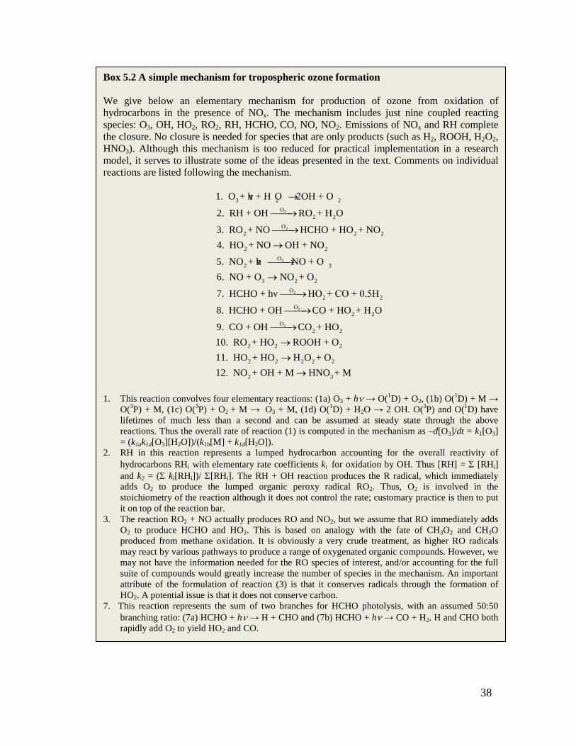
Box 5.2 A simple mechanism for tropospheric ozone formation We give below an elementary mechanism for production of ozone from oxidation of hydrocarbons in the presence of NOx. The mechanism includes just nine coupled reacting species: O3, OH, HO2, RO2, RH, HCHO, CO, NO, NO2. Emissions of NOx and RH complete the closure. No closure is needed for species that are only products (such as H2, ROOH, H2O2, HNO3). Although this mechanism is too reduced for practical implementation in a research model, it serves to illustrate some of the ideas presented in the text. Comments on individual reactions are listed following the mechanism.

2

2

2

2

2

3 2 2O

2 2O

2 2 2

2 2O

2 3

3 2 2O

2 2O

1. O + hν + H O 2OH + O

2. RH + OH RO + H O

3. RO + NO HCHO + HO + NO4. HO + NO OH + NO

5. NO + hν NO + O6. NO + O NO + O

7. HCHO + hν HO + CO + 0.5H

8. HCHO + OH CO + HO

→

→

→→

→→

→

→2

2 2O

2 2

2 2 2

2 2 2 2 2

2 3

+ H O

9. CO + OH CO + HO10. RO + HO ROOH + O11. HO + HO H O + O12. NO + OH + M HNO + M

→→→

→

1. This reaction convolves four elementary reactions: (1a) O3 + hν → O(1D) + O2, (1b) O(1D) + M →

O(3P) + M, (1c) O(3P) + O2 + M → O3 + M, (1d) O(1D) + H2O → 2 OH. O(3P) and O(1D) have

lifetimes of much less than a second and can be assumed at steady state through the above reactions. Thus the overall rate of reaction (1) is computed in the mechanism as –d[O3]/dt = k1[O3] = (k1ak1d[O3][H2O])/(k1b[M] + k1d[H2O]).

2. RH in this reaction represents a lumped hydrocarbon accounting for the overall reactivity of hydrocarbons RHi with elementary rate coefficients ki for oxidation by OH. Thus [RH] = Σ [RHi] and k2 = (Σ ki[RHi])/ Σ[RHi]. The RH + OH reaction produces the R radical, which immediately adds O2 to produce the lumped organic peroxy radical RO2. Thus, O2 is involved in the stoichiometry of the reaction although it does not control the rate; customary practice is then to put it on top of the reaction bar.

3. The reaction RO2 + NO actually produces RO and NO2, but we assume that RO immediately adds O2 to produce HCHO and HO2. This is based on analogy with the fate of CH3O2 and CH3O produced from methane oxidation. It is obviously a very crude treatment, as higher RO radicals may react by various pathways to produce a range of oxygenated organic compounds. However, we may not have the information needed for the RO species of interest, and/or accounting for the full suite of compounds would greatly increase the number of species in the mechanism. An important attribute of the formulation of reaction (3) is that it conserves radicals through the formation of HO2. A potential issue is that it does not conserve carbon.

7. This reaction represents the sum of two branches for HCHO photolysis, with an assumed 50:50 branching ratio: (7a) HCHO + hν → H + CHO and (7b) HCHO + hν → CO + H2. H and CHO both rapidly add O2 to yield HO2 and CO.

39

The choice of species to be included in the coupled chemical mechanism must involve a balance between chemical completeness and computational requirements. Although experience and chemical intuition are important in the construction of a chemical mechanism, one can also use objective considerations. Consider for example the construction of a chemical mechanism to compute OH radical concentrations in the troposphere We know that tropospheric OH has a concentration ~106 molecules cm-3 and a lifetime ~1 s. It follows that the important reactions controlling OH must have rates ~ 106 molecules cm-3 s-1. Species for which total production rates (Pi) and loss rates (ℓini) are orders of magnitude lower under the conditions of interest will not play a significant role in OH chemistry, either directly or indirectly, and can thus be decoupled or eliminated from the mechanism. Starting from a large ensemble of candidate species, it is thus possible to construct objectively a reduced mechanism. Calculations of Pi and ℓini can be made locally in a CTM so that reduced mechanisms adapted to the local conditions can be selected (Santillana et al., 2010).