radar target classification using support vector machines
TRANSCRIPT

IN DEGREE PROJECT MATHEMATICS,SECOND CYCLE, 30 CREDITS
, STOCKHOLM SWEDEN 2017
Radar target classification using Support Vector Machines and Mel Frequency Cepstral Coefficients
SEBASTIAN EDMAN
KTH ROYAL INSTITUTE OF TECHNOLOGYSCHOOL OF ENGINEERING SCIENCES


Radar target classification using Support Vector Machines and Mel Frequency Cepstral Coefficients EDMAN SEBASTIAN Degree Projects in Optimization and Systems Theory (30 ECTS credits) Degree Programme in Applied and Computational Mathematics (120 credits) KTH Royal Institute of Technology year 2017 Supervisors at SAAB: Stefan Eriksson, Niklas Broman Supervisor at KTH: Johan Karlsson Examiner at KTH: Johan Karlsson

TRITA-MAT-E 2017:63 ISRN-KTH/MAT/E--17/63--SE Royal Institute of Technology School of Engineering Sciences KTH SCI SE-100 44 Stockholm, Sweden URL: www.kth.se/sci

SF280X Master Thesis
Abstract
In radar applications, there are often times when one does not only want to knowthat there is a target that reflecting the out sent signals but also what kind oftarget that reflecting these signals. This project investigates the possibilities tofrom raw radar data transform reflected signals and take use of human perception,in particular our hearing, and by a machine learning approach where patternsand characteristics in data are used to answer the earlier mentioned question.More specific the investigation treats two kinds of targets that are fairly compa-rable namely smaller Unmanned Aerial Vehicles (UAV) and Birds. By extractingcomplex valued radar video so called I/Q data generated by these targets usingsignal processing techniques and transform this data to a real signals and af-ter this transform the signals to audible signals . A feature set commonly usedin speech recognition namely Mel Frequency Cepstral Coefficients are used twodescribe these signals together with two Support Vector Machine classificationmodels. The two models where tested with an independent test set and the linearmodel achieved a overall prediction accuracy 93.33 %. Individually the predictionresulted in 93.33 % correct classification on the UAV and 93.33 % on the birds.Secondly a radial basis model with a overall prediction accuracy of 98.33 % whereachieved. Individually the prediction resulted in 100% correct classification onthe UAV and 96.76 % on the birds. The project is partly done in collaborationwith J. Clemedson [2] where the focus is, as mentioned earlier, to transform thesignals to audible signals.

Master Thesis SF280X
Sammanfattning
Klassificiering utav radarmål genom Support Vector Machinesoch Mel Frequency Cepstral Coefficients
I radar applikationer räcker det ibland inte med att veta att systemet observeratett mål när en reflekted signal dekekteras, det är ofta också utav stort instresseatt veta vilket typ av föremål som signalen reflekterades mot. Detta projektundersöker möjligheterna att utifrån rå radardata transformera de reflekteradesignalerna och använda sina mänskliga sinnen, mer specifikt våran hörsel, föratt skilja på olika mål och också genom en maskininlärnings approach där medhjälp av mönster och karaktärsdrag för dessa signaler används för att besvarafrågeställningen. Mer ingående avgränsas denna undersökning till två typer avmål, mindre obemannade flygande farkoster (UAV) och fåglar. Genom att ex-trahera komplexvärd radar video även känt som I/Q data från tidigare nämndatyper av mål via signalsbehandlingsmetoder transformera denna data till reellasignaler, därefter transformeras dessa signaler till hörbara signaler. För att klas-sificera dessa typer av signaler används typiska särdrag som också används inomtaligenkänning, nämligen, Mel Frequency Cepstral Coefficients tillsammans medtvå modeller av en Support Vector Machine klassificerings metod. Med den lin-jära modellen uppnåddes en prediktions nogrannhet på 93.33%. Indivudiellt varnogrannhetern 93.33 % korrekt klassificiering utav UAV:n och 93.33 % på fåglar.Med radial bas modellen uppnåddes en prediktions noggrannhet på 98.33%. Indi-viduellt var noggrannheten 100% korrekt klassificiering utav UAV:n och 96.76%på fåglar. Projektet är delvis utfört med J. Clemedson [2] vars fokus är att, somtidigare nämnt, transformera dessa signaler till hörbara signaler.


SF280X Master Thesis
Acknowledgement
I would like to thank my supervisor Johan Karlsson, associate professor at thedepartment of mathematics at KTH for supervising this thesis and by discussingideas and giving feedback resulting to a thesis at the best of my abilities.
I wound also like to thank my two supervisors as SAAB, Stefan Eriksson andNiklas Broman. When staring this thesis my knowledge for radar system wheresmall or even close to zero. By always taking time to answer my questions andgive feedback on my reflections I’ve broaden my knowledge further to a directionwho was not the main area in my field of study.
Thanks to friends and family for supporting me not only during this thesisbut also under my five years at KTH. Lastly a sincere thanks to Johan Clemed-son for his collaboration in this project.
Stockholm, August 2017Sebastian Edman


Master Thesis SF280X
Contents
1 Introduction and Problem Description 31.1 Outline of Thesis . . . . . . . . . . . . . . . . . . . . . . . . . . . 4
2 Background on RADAR technology 52.1 Pulse radar sets . . . . . . . . . . . . . . . . . . . . . . . . . . . . 52.2 Antenna . . . . . . . . . . . . . . . . . . . . . . . . . . . . . . . . 62.3 Transmitter . . . . . . . . . . . . . . . . . . . . . . . . . . . . . . 82.4 Transmission of signal . . . . . . . . . . . . . . . . . . . . . . . . 82.5 Radar equation . . . . . . . . . . . . . . . . . . . . . . . . . . . . 92.6 Range and Bearing . . . . . . . . . . . . . . . . . . . . . . . . . . 102.7 Radar resolution . . . . . . . . . . . . . . . . . . . . . . . . . . . 112.8 Doppler effect . . . . . . . . . . . . . . . . . . . . . . . . . . . . . 12
2.8.1 In-phase/Quadrature demodulation . . . . . . . . . . . . . 142.8.2 µ−Doppler effect . . . . . . . . . . . . . . . . . . . . . . . 16
3 Signal Processing Background 183.1 Filters . . . . . . . . . . . . . . . . . . . . . . . . . . . . . . . . . 18
3.1.1 FIR Filters . . . . . . . . . . . . . . . . . . . . . . . . . . 183.1.2 Matched Filter . . . . . . . . . . . . . . . . . . . . . . . . 19
3.2 Spectral Transforms . . . . . . . . . . . . . . . . . . . . . . . . . 223.2.1 Discrete Fourier Transform . . . . . . . . . . . . . . . . . 22
3.3 Features . . . . . . . . . . . . . . . . . . . . . . . . . . . . . . . . 233.3.1 Mel Frequency Cepstral Coefficients . . . . . . . . . . . . 23
4 Classification Method 254.1 Support Vector Machines (SVM) . . . . . . . . . . . . . . . . . . 254.2 Dual Formulation . . . . . . . . . . . . . . . . . . . . . . . . . . . 274.3 Kernel Trick . . . . . . . . . . . . . . . . . . . . . . . . . . . . . . 28
5 Radar Signal Processing 305.1 MTI-filter . . . . . . . . . . . . . . . . . . . . . . . . . . . . . . . 315.2 Pulse Compression . . . . . . . . . . . . . . . . . . . . . . . . . . 325.3 Signal Extraction . . . . . . . . . . . . . . . . . . . . . . . . . . . 335.4 Spectral Modifications . . . . . . . . . . . . . . . . . . . . . . . . 34
6 Data Sets and Implementation 376.1 Data Set . . . . . . . . . . . . . . . . . . . . . . . . . . . . . . . . 376.2 Implementation . . . . . . . . . . . . . . . . . . . . . . . . . . . . 376.3 Training and Parameter Evaluation . . . . . . . . . . . . . . . . . 39
7 Results 41
8 Discussion and Future Work 45

SF280X Master Thesis
A Appendix A 47A.1 Resampling . . . . . . . . . . . . . . . . . . . . . . . . . . . . . . 47
A.1.1 Up-Sampling by integer factor . . . . . . . . . . . . . . . . 47A.1.2 Interpolation Filter . . . . . . . . . . . . . . . . . . . . . . 50A.1.3 Polyphase Interpolation filter . . . . . . . . . . . . . . . . 51A.1.4 Down-sampling (or Decimation) by an Integer Factor . . . 52A.1.5 Resampled with non-integer factor . . . . . . . . . . . . . 52A.1.6 Kaiser window . . . . . . . . . . . . . . . . . . . . . . . . 52

Master Thesis SF280X
Nomenclature
(·)H Hermitian transpose
α Lagrange multipliers
∗ Convolution
β0 bias
β Weight vector
λ Wave Length
σt Radar Cross Section
τ Pulse Width
c Speed of light
f0 Carrier frequency
fD Doppler frequency
G Antenna Gain
h[·] Impulse response
Ls Loss factor
P Signal power
SA Angular resolution
Sr Range resolution
1

SF280X Master Thesis
Acronyms
CC Cepstral Coefficients.CW Continuous Wave.
DFT Discrete Fourier Transform.DTW Dynamic Time Wrapping.
FIR Finite Impulse Response.
HMM Hidden Markov Models.
IDFT Inverse Discrete Fourier Transform.
LOS Line Of Sight.LSS Low, Slow flying and Small.
MDS Minimum Discernible Signal.MFCC Mel Frequency Cepstral Coefficients.MTI Moving Target Indicator.
PRF Pulse Repetition Frequency.PRT Pulse Repetition Time.
RF Radio Frequency.
SNR Signal to Noise Ratio.SVM Support Vector Machine.
TX Transmission.
UAV Unmanned Aerial Vehicles.
2
Master Thesis SF280X
1 Introduction and Problem Description
The radar has for more than half a century been the go to technology for surveil-lance and target recognition. This is due to the many advantages of radar sys-tems, for example a radar system can detect and track moving objects in allweathers during day and night. A radar transmits and receives electromagneticwaves, that interacts with targets and the surrounding environment. The ve-locity of moving targets can be calculated by measuring the Doppler frequencyshift of the received echo signal. Detecting the target is often not enough, onealso wants to distinguish between targets. In today’s radar systems this can bedone in various ways, for example discriminate targets by their velocity or spe-cific motion patterns which are unique for a target. Such methods are almostas old as the radar itself and in later years more sophisticated methods havebeen developed by the use of machine learning algorithms, for example imageclassification in Synthetic Aperture Radar (SAR). But classification is not neces-sary performed in an automatic approach. Some radar system, possess an audiooutput. For example the MSTAR Battlefield Surveillance Radar, which is a manportable lightweight Doppler radar used by an operator who can listen to theaudio output. The audio signal is a representation of the echo from the illumi-nated target which contains the Doppler frequencies. The operator makes theclassification by recognize specific patterns in the audio signal, which is similarto the techniques used in SONAR applications. The operators ability to performauditory classification is based on speech phonemics principles. A phoneme is aspecific sound pattern that the human brain is able to recognize. For the opera-tor to be able do distinguish between different targets (and also specific actionsby targets) extensive training is needed. The human factor may also increasethe error rate, especially on the battlefield where external factors can have animpact on the human senses. Today it exist speech recognition methods like Dy-namic Time Wrapping (DTW) and Hidden Markov Models (HMM). But thosemethods have been optimized for speech signals and the aural Doppler signal isnot a conventional speech signal. Another challenge may be to classify targetsduring the scan of a surveillance radar which results in rather short time framesof the signal (milliseconds) and contains relatively long discontinuities betweenthe frames. This can lead to that existing methods may be possible to use ina mode when the radar stares at a target but does not imply that it would bepossible to use in scanning mode.
The overall aim of this project is to investigate the possibilities to transformradar data to an aurial output and make use of feature driven classification al-gorithms based on aurial signals to discriminate between Low, Slow flying andSmall (LSS) targets such as smaller Unmanned Aerial Vehicles (UAV) and birdsthat is fairly comparable (size, velocity, flight pattern) and thus hard to distin-guishing between in a radar system application. The project has three mainparts, and is partly done in collaboration with J. Clemedson. The included partsis stated as follows.
i) From raw radar data, with help of signal processing techniques extract sig-
3

SF280X Master Thesis
nals from UAV:s and birds
ii) Transform those signals so it would be possible for an operator to listen toan aurial signal
iii) Based on these aurial signals, develop an automatic classification method onthe same theme to serve as supplement to the operator
Part i) is done in collaboration with J. Clemedson and included in this thesis,part ii) can be found in [2] and part iii) are alone included in this thesis.
1.1 Outline of Thesis
The thesis contains 8 Sections. Section 2 treats basic radar technology includingtransmission of signals, range measurements and the Doppler effect. In Section3 signal processing techniques are introduced that are used in the thesis. Sec-tion 4 treats theory on the Support Vector Machine classification method andsubjects like duality and kernel trick. Section 5 describes the process used forextracting radar data from complex raw radar video, so called I/Q data. Insection 6 the datasets for classification are described and the implementation ofthe classification method training phase is outlined. In Section 7 the result fromthe classification is presented and finally in Section 8 some own thoughts on theproject and future work are discussed. Section 2, 3 (except 3.3) and 5 are donein collaboration with J. Clemedson.
4
Master Thesis SF280X
2 Background on RADAR technology
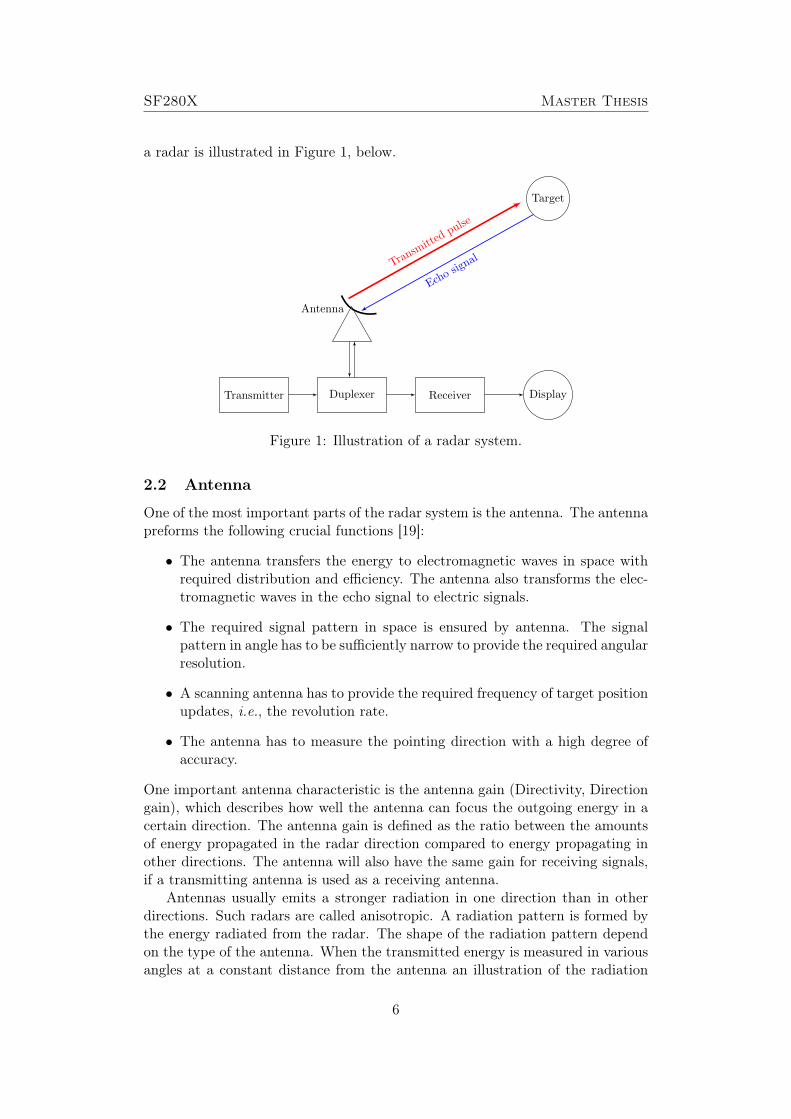
A radar (RAdio Detecting And Ranging) transmits electricmagnetic energy inthe radio-frequency (RF) interval. When the transmitted RF energy hits a targetthe energy is reflected. The radar receives a small quantity of the reflected energy,called the echo, which is used to determine the distance and direction of theobject. This section aims to introduce some basic radar theory needed understandthe terminology used in this thesis. For starters general signal transmission isintroduced with theory gathered from [18] and the included components in aradar system from [19] and [21] then general range measurements in a radarsystem from [20].
Radar systems can be divided in to two different types of radar systems, pri-mary and secondary radar systems. Primary radar systems transmits a signaland receives the reflected echo. While secondary radar systems receives an codedreply signal from an transmitter on the illuminated targets. Hence secondaryradar systems are not used to detect unknown targets but instead tracking andidentifying friendly targets. Primary radar systems are divided into Continu-ous Wave (CW) and pulsed radar systems. A CW radar set transmits a highfrequency signal continuously, the received echo signal is also processed contin-uously. CW radars can normally only measure the targets speed and not thedistance to targets, since there are no pulse sets to time. This problem can besolved by constantly shifting the frequency in the transmitted signal. These fre-quencies can be extracted from the echo and by knowing when in the past thatparticularly frequency was sent out, one can do a range calculation. This types ofCW radar sets are called frequency modulated CW radars, hence CW radar setscan be divided in modulated and unmodulated CW radar systems. The typicaluse of unmodulated CW radar sets, which only can measure speed, are speedgauges for the police.
Pulse radar transmits a high frequency impulse signal of high power, afterthe impulse a longer break follows in which the echoes are received before thennext impulse is sent out. Properties such as direction, range and speed can bedetermined by using a pulse radar. The following theory will only consider pulseradar theory.
2.1 Pulse radar sets
A powerful transmitter generates the radar signal, which is transmitted fromantenna through a duplexer. The function of the duplexer is to switch the an-tenna between the transmitter and receiver, which means that only one antennais needed. Switching between transmitting and receiving signals is also neces-sary, since the high power pulses produced by the transmitter would destroy thereceiver if energy were allowed to enter the receiver during transmission. Theantenna illuminates the target with the radio frequency pulse, which is reflectedat the target. The backscattered echo signal is picked up by the receiver in theantenna. The received radar pules is amplified and demodulated in the receiver,which produces video signals that can be displayed. The operating principles of
5
SF280X Master Thesis
a radar is illustrated in Figure 1, below.
Transmitter Duplexer Receiver Display
Target
Antenna
Transm
itted
pulse
Echo
signal
Figure 1: Illustration of a radar system.
2.2 Antenna
One of the most important parts of the radar system is the antenna. The antennapreforms the following crucial functions [19]:
• The antenna transfers the energy to electromagnetic waves in space withrequired distribution and efficiency. The antenna also transforms the elec-tromagnetic waves in the echo signal to electric signals.
• The required signal pattern in space is ensured by antenna. The signalpattern in angle has to be sufficiently narrow to provide the required angularresolution.
• A scanning antenna has to provide the required frequency of target positionupdates, i.e., the revolution rate.
• The antenna has to measure the pointing direction with a high degree ofaccuracy.
One important antenna characteristic is the antenna gain (Directivity, Directiongain), which describes how well the antenna can focus the outgoing energy in acertain direction. The antenna gain is defined as the ratio between the amountsof energy propagated in the radar direction compared to energy propagating inother directions. The antenna will also have the same gain for receiving signals,if a transmitting antenna is used as a receiving antenna.
Antennas usually emits a stronger radiation in one direction than in otherdirections. Such radars are called anisotropic. A radiation pattern is formed bythe energy radiated from the radar. The shape of the radiation pattern dependon the type of the antenna. When the transmitted energy is measured in variousangles at a constant distance from the antenna an illustration of the radiation
6

Master Thesis SF280X
pattern can be plotted, usually in polar coordinates. In such plots three keyfeatures can be observed:
• In the region that is within 3 dB of the maximum radiation, is called themain lobe or main beam.
• Smaller beams in other directions than the main lobe are called sidelobes,which are usually radiation in undesired directions. These sidlobes cannever be completely eliminated.
• The portion of the radiation pattern that are directed in the opposite di-rection of the main lobe is called the backlobe.
One important characteristic of the radiation pattern is the beam width. Thebeam width is defined as the angular range of the radiation pattern in which atleast half of the maximum power is still emitted. Hence the bordering points ofthe lobe are therefore the points at which the field strength fallen 3 dB comparedto the maximum field strength. The notation of the beam width (or half powerangle) is Θ. The beam width can be determined in both the horizontal ΘAZ andvertical plane ΘEL.
The ratio of power gain between the main lobe and the backlobe is called thefront to back ratio. One desires a high front to back ratio, since its means thata minimum amount of energy is radiated in the undesired direction.
Air-surveillance radar system usually uses a cosecant squared pattern, toachieve a more uniform signal strength from a target that moves with a constantelevation. The height information from a detection can be calculated by knowingthe elevation of the returned echo. This is done with the agile multiple beamconcept, where the height information is divided into multiple parts (beams),see Figure 2. The cosecant squared pattern can be achieved by stacking beamsaccording to the figure.
Figure 2: Illustration of cosecant pattern [17]
7

SF280X Master Thesis
2.3 Transmitter
The task of the transmitter is to produce high power Radio Frequency (RF) pulsesof energy that are radiated into space by the antenna. There are different kindsof transmitter with different properties. Depending on what type of transmitterused in the radar set, the radar set can be classified as coherent or non-coherent[21]. The radar system is said to be coherent if every transmitted pulse starts withthe same phase and non-coherent if the phase of each successive pulse is random.The reason to use a coherent system is to keeping track of the phase change of thereflected pulses generated by a moving target and hence the Doppler frequencies.Radars that emit coherent pulses to measure the Doppler shift are known aspulse Doppler radars. The difference between coherent and non-coherent pulsescan be seen in Figure 3.
(a) Coherent pulses (b) Non-coherent pulses
Figure 3: Illustration of coherent and non-coherent radar transmitters.
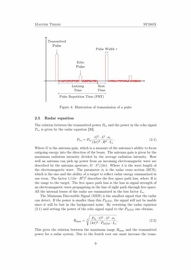
2.4 Transmission of signal
Each transmitting pulse is radiated from the radar, during the transmit time (orpulse width τ). The radar is waiting for return echo during the listening time,after each transmitted pules. There is a short rest time between the listeningtime and the next pulse. The time between two pulses are called the PulseRepetition Time (PRT). The number of pulses transmitted per second is calledPulse Repetition Frequency (PRF), the relationship between the pulse repetitiontime and pulse repetitive frequency is given by PRT = PRF−1. An illustrationof a transmission of a pulse with previously mentioned variables can be seen inFigure 4.
8
Master Thesis SF280X
Transmitted
Pulse
Echo
Pulse
Pulse Width τ
ListningTime
RestTime
Pulse Repetition Time (PRT)
Figure 4: Illustration of transmission of a pulse
2.5 Radar equation
The relation between the transmitted power Ptx and the power in the echo signalPrx is given by the radar equation [20],
Prx = PtxG2 · λ2 · σt
(4π)3 ·R4 · Ls. (2.1)
Where G is the antenna gain, which is a measure of the antenna’s ability to focusoutgoing energy into the direction of the beam. The antenna gain is given by themaximum radiation intensity divided by the average radiation intensity. Howwell an antenna can pick up power from an incoming electromagnetic wave aredescribed by the antenna aperture, G · λ2/(4π). Where λ is the wave length ofthe electromagnetic wave. The parameter σt is the radar cross section (RCS),which is the size and the ability of a target to reflect radar energy summarized inone term. The factor 1/(4π ·R2)2 describes the free space path loss, where R isthe range to the target. The free space path loss is the loss in signal strength ofan electromagnetic wave propagating in the line of sight path through free space.All the internal losses of the radar are summarized in the loss factor Ls.
The Minimum Discernible Signal (MDS) is the smallest signal that the radarcan detect. If the power is smaller than this PMDS , the signal will not be usablesince it will be lost in the background noise. By rewriting the radar equation(2.1) and setting the power of the echo signal equal to the PMDS one obtains,
Rmax = 4
√Ptx ·G2 · λ2 · σt
(4π)3 · PMDS · Ls. (2.2)
This gives the relation between the maximum range Rmax and the transmittedpower for a radar system. Due to the fourth root one must increase the trans-
9
SF280X Master Thesis
mitted power 16 times to double the maximum range, if the other parametersare constant.
2.6 Range and Bearing
The slant range R is defined as the line of site distance between the target andthe radar antenna. It is possible to calculate the slant range from the timedelay tdelay between the transmitted and the reflected pulse, with the followingequation
R =ctdelay
2, (2.3)
where c is the speed of light. It is required to know the target’s elevation tocalculate the horizontal distance between the target and radar (ground range).
Since a pulse radar usually transmits a sequence of pulses and measures thetime between the last transmitted pules and the echo pulse. It is possible thatthe received echo is from a long range target, so that the received signal arrives atthe radar after or during the transmission of the next transmitting pulse. Thismeans that the radar is measuring the wrong time interval and therefore thewrong range. The radar assumes that the pulse is the reflection of the secondtransmitted pulse and declares a reduced range for the target. This occurs whenstrong targets are located outside the range that corresponds to the pulse rep-etition time, and are called range ambiguity. Hence a maximum unambiguityrange is defined by the pulse repetition time. The relationship between the pulserepetition time and the unambiguity range Ruamb is given by
Ruamb =(PRT − τ)c
2. (2.4)
There are two types of echo signals that arrives after the reception time:
• Echo signals that arrives during the transmission time. These signals willnot be registered since the receiver is turned off during transmission.
• Echo signals that arrives during the following reception time. These signalswill give range measuring failures (ambiguous returns) illustrated in Figure5
Still, it is possible to discriminate the true range of targets by using differentTransmission (TX) modes. The different transmission modes have various pulsepulse repetition frequencies (PRF) explained in Section 2.4. Hence targets atambiguous ranges will appear at different ranges for each TX-mode allowing theradar system to compute and solve the ambiguity and extract the true range.
10

Master Thesis SF280X
U
0 10 20 0 10 20 0 10 km
40
10
Figure 5: Illustration of range measuring failure
There is also a minimum detectable rage (or blind distance) to consider. This isdue to that the echo signal will not be registered, if the echo from the beginningof the pulse falls inside the transmitting pulse. Since the receiver is turned offduring the transmitting time. The blind distance can be calculated with thefollowing equation,
Rmin =(τ + trest)c
2, (2.5)
where trest is the resting time. Both the horizontal and elevation angel betweenthe antenna and target, can be determined by measuring the direction in whichthe antenna is pointing when the echo is received. The accuracy of the radarsangular measurements is determined by the antennas directional gain. The anglemeasured in the horizontal plane is refereed to as bearing, which can be measuredin true or relative bearing. True bearing is the angle between the true north anda line pointing directly at the target, measured in a clockwise direction. Relativebearing is the angle between the centerline of the own ship ore aircraft and atarget, measured in a clockwise direction.
2.7 Radar resolution
A radar is not able to distinguish between targets that are very close in bearingor range. The ability to distinguish between close target are given by the targetresolution of the radar, which is divided in angular resolution and range resolu-tion. The minimum angular separation of two equal targets at the same range,are called angular resolution. The angular resolution of an radar is determinedby the half power beam width Θ of the radar. Which is the angle between thehalf power (-3 dB) points of the main lobe. Which means that two targets canbe resolved in angle if they are separated more than one beam width. Hence thesmaller the beam width, the higher directivity of the antenna, the better angu-lar resolution. The distance between two targets corresponding to the angularresolution is a function of the slant range and given by,
SA = 2R sinΘ
2. (2.6)
Where SA is the angular resolution given as a distance between two targets.
11

SF280X Master Thesis
The ability to distinguish between two or more targets at different ranges buton the same bearing, is called range resolution. The range resolution is a factorsince the echo’s from close targets in range gets mixed up as illustrated in Figure6.
τ = 1µs300m 100m
��
��
��
��
��
��
��
(a) Targets mixed up in the same echo
τ = 1µs300m 200m
��
��
��
��
��
��
��
(b) Targets separated by two echoes
Figure 6: Illustration of range resolution
Hence the primary factor in range resolution is the pules width of the transmittedpulse. But the range resolution also depends on types and sizes of the target,and the efficiency of the receiver and indicator. Targets separated by half thepulse width, can be separate distinguished by an well designed radar with allother factors at maximum efficiency. Hence, the theoretical range resolution of aradar system is given by
Sr =cτ
2. (2.7)
Where Sr is the range resolution given as distance between two targets. A methodto improve the range resolution is by using a pulse compression system, usingpulse compression allows high range resolution with long pulses, but with a higheraverage power
2.8 Doppler effect
The Doppler effect was discovered by Christan Doppler 1842 and has been usedin electromagnetic since 1930 and the first Doppler radar was produced in 1950.The use of the Doppler radar is mainly for targets in motion e.g in militaryuse targets of interest can be hostile air, sea and land targets such as airplanes,ships and tanks but also smaller targets like rockets, artillery and mortars. Theprinciple behind the Doppler shift is that a target with a motion relative tothe radar will induce a frequency shift in the reflected signal i.e the Dopplershift which depends on the wavelength of the transmitted signal and the radialvelocity (the velocity in the Line Of Sight (LOS) of the radar), of the illuminatedtarget. Suppose that the transmitted signal is
12

Master Thesis SF280X
st(t) = u(t) cos(2πf0t) (2.8)
where u(t) is the signal envelope, f0 is the carrier frequency, and t is the time.The received backscattered echo signal from a target can then be expressed as
sr(t) = σst(t− tr) = σu(t− tr) cos(2πf0(t− tr)) (2.9)
where σ is the target reflection coefficient and tr is the time delay of the echow.r.t the transmitted signal. If the target would be stationary relative to theradar the time delay would be constant and also the phase of the echo signal. Ifthe target would be in motion relative to the radar with a velocity vr in the lineof sight of the radar the echo signal received at time t transmitted at time t− trand the the time that the target is illuminated is ti = t − tr/2 and hence thedistance between the origin of the radar and the illuminated target is
R(ti) = R0 − vrti (2.10)
where R0 is the distance between the origin of the radar and the illuminatedtarget at time t = 0. The propagation time of the signal for traveling the distancefrom the radar to the target and back is the time delay of the echo tr and thus
tr =2R(ti)
c(2.11)
where c is the speed of light in the case of electromagnetic waves. By combining(2.10) with (2.11) and substitution into the echo signal (2.9) yields
sr(t) = σu(tc+ vrc− vr
− 2R0
c− vr
)cos
[2πf0
(tc+ vrc− vr
− 2R0
c− vr
)](2.12)
The echo signal (2.12) possesses two important properties [24]
i) From the phase term of (2.12) one can see that the frequency is shifted fromf0 to f0
c+vrc−vr
ii) There is a scaling change for the echo signal envelope in terms of time.
The envelope change of the echo signal described in ii) can in most radar appli-cations be ignored since the process of the phase term will not heavily dependon the scaling change of the echo signal envelope [24].
Usually the radial velocity vr of the illuminated target is significantly smallerthan the propagation speed of an electromagnetic wave c thus one can argue toapproximate the frequency shift
f0c+ vrc− vr
− f0 = f02vrc− vr
≈ f02vrc
=2vrλ0
. (2.13)
Where λ0 is the carrier wavelength, the right hand side in (2.13) is the definedas the Doppler frequency
13

SF280X Master Thesis
fD =2vrλ0
. (2.14)
If (2.14) combined with (2.13) is inserted in (2.12) and assume that the envelopeof the signal u(s) = 1 we arrive at
sr(t) = σ cos
[2π(f0 + fD)t− f0
2R0
c− vr
]= σ cos
[2π(f0 + fD)t− θ
]= σ cos
[2πf0t+ φ(t)− θ
].
(2.15)
In order to distinguish between positive and negative Doppler frequencies, anI/Q representation of the signal is used and introduced in the next section.
2.8.1 In-phase/Quadrature demodulation
In Doppler radar applications it is of great importance to be able to distin-guish between positive and negative frequencies. Since the sign of the Dopplerfrequency represents in which direction the targets is moving. But a signal repre-sentation just using a series of samples of the momentary amplitude of the signal(see Figure 7a), will not be able to distinguish between positive and negativefrequencies (for example cos(x) = cos(−x)). Hence the In-phase/Quadrature(I/Q) representation of the signal is introduced. Where the signal is compared toa reference signal which gives an in-phase (I) component and a quadrature (Q)component of the signal [9]. The I/Q-signal can be illustrated as spiral in threedimensions, see Figure 7b.
0 100 200 300 400 500 600 700-1
-0.8
-0.6
-0.4
-0.2
0
0.2
0.4
0.6
0.8
1
cos(x)
x
(a) Projection of I/Q representation
0 100 200 300 400 500 600 700
-1
-0.5
0
0.5
1-1
-0.5
0
0.5
1
xQ-part
I-part
(b) I/Q representation
Figure 7: Signal representation
One can see that the projection of the spiral on to the vertical plane is the "real"signal (Figure 7a), which is the I component. The projection of the spiral on to
14
Master Thesis SF280X
the vertical plane gives the Q component of the signal. The direction of rotationof the spiral in Figure 7b determines the sign of the frequency.
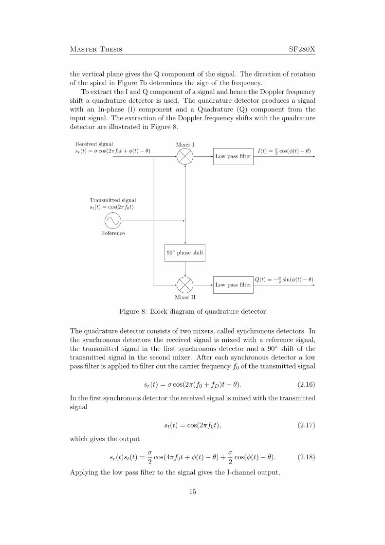
To extract the I and Q component of a signal and hence the Doppler frequencyshift a quadrature detector is used. The quadrature detector produces a signalwith an In-phase (I) component and a Quadrature (Q) component from theinput signal. The extraction of the Doppler frequency shifts with the quadraturedetector are illustrated in Figure 8.
Received signalsr(t) = σ cos(2πf0t+ φ(t) − θ)
Mixer I
Transmitted signalst(t) = cos(2πf0t)
Reference
90◦ phase shift
Mixer II
Low pass filter
Low pass filter
I(t) = σ2 cos(φ(t) − θ)
Q(t) = −σ2 sin(φ(t) − θ)
Figure 8: Block diagram of quadrature detector
The quadrature detector consists of two mixers, called synchronous detectors. Inthe synchronous detectors the received signal is mixed with a reference signal,the transmitted signal in the first synchronous detector and a 90◦ shift of thetransmitted signal in the second mixer. After each synchronous detector a lowpass filter is applied to filter out the carrier frequency f0 of the transmitted signal
sr(t) = σ cos(2π(f0 + fD)t− θ). (2.16)
In the first synchronous detector the received signal is mixed with the transmittedsignal
st(t) = cos(2πf0t), (2.17)
which gives the output
sr(t)st(t) =σ
2cos(4πf0t+ φ(t)− θ) +
σ
2cos(φ(t)− θ). (2.18)
Applying the low pass filter to the signal gives the I-channel output,
15
SF280X Master Thesis
I(t) =σ
2cos(φ(t)− θ). (2.19)
In the other synchronous detector, the 90◦ phase shifted transmitted signal,
s90◦t (t) = sin(2πf0t) (2.20)
which gives the output
sr(t)s90◦t (t) =
σ
2sin(4πf0t+ φ(t)− θ)− σ
2sin(φ(t)− θ). (2.21)
Applying the low pass filter to the signal gives the Q-channel output,
Q(t) = −σ2
sin(φ(t)− θ). (2.22)
By combining the I and Q part the following signals is obtained
sD(t) = I(t) + iQ(t) =σ
2e−iφ(t)−θ =
σ
2e−i2πfDt−θ. (2.23)
From the complex Doppler signal in Equation (2.23) it is possible in to extractpositive and negative frequencies, i.e. positive and negative velocities.
2.8.2 µ−Doppler effect
By extract information about the illuminated target via the Doppler shift interms of radial velocity and range useful information is gained, but in real radarapplications targets with single motion pattern is quite rare. For example manmade aerial targets like helicopters and UAV:s consist of more complex motionsthan just the bulk motion, like engine vibrations and rotations of propellers. Andbiological targets such as personnel or birds generates complementary motionslike swinging arms and flapping wings. These so called micro-motions can beuseful when trying to distinguish between many more classes of targets men-tion above and even different types of the same kind of target due to uniquecharacteristics. Pursuant to Doppler theory beyond the bulk motion of a targetmicro-motions from parts of the target or the target itself can cause frequencymodulation on the echo signal from a radar system. Which is in fact a Dopplersideband besides the main Doppler frequency induced by the bulk motion of thetarget [24]. These frequency modulations generated by micro-motions are in lit-erature and research called micro-Doppler effect and a target is said to have aspecific micro-Doppler signature.
The micro-Doppler effect has its origin in coherent laser detecting and rangingsystems (LADAR) [1] who transmit electromagnetic waves at optical frequenciesand by the backscattered wave from an object one can measure properties suchas range, velocity similar to a radar system by preserve phase information. Sincethe phase of a backscattered signal in a coherent system is sensitive to the vari-ation in range a half wavelength change in range can cause 2π change in phase.In LADAR systems where the wavelengths is typically short e.g 2 µm and thus a
16

Master Thesis SF280X
change in radial distance by 1 µm can generate a shift in phase by 2π leading toextremely high sensitivity in LADAR systems where for example tiny vibrationscan be observed rather easily. The micro-Doppler frequency is a time varyingproperty and can be extracted from the output from a quadrature detector usedin standard Doppler processing [1].
The author of [1] [24] validated the µ−Doppler effect in radar systems by usingan X-band radar to detect trigonometric scatter target with a vibration am-plitude of 1 mm and vibration frequency of 10 Hz and successfully extractedmicro-Doppler frequency shift through time-frequency analysis technique, lateron the concerned also put forth results of micro-Doppler analysis results of apedestrian with X-band radar. Since then many papers related to the researchfield have been published, not only in the research of micro-Doppler but alsowith the previous combined with various classification methods. The authorsof [14] uses a speech recognitions techniques, Dynamic Time Wrapping (DTW)and a k -NN classifier to classify baseband audio output signal from a radar withhelp of micro-Doppler signatures. Speech processing algorithms exploit the timevariance in speech patterns to classify signals and identify words and the intendwas to exploit the time variance in the micro-Doppler signature in a similar man-ner. Here the classification set consisted of three classes namely wheeled vehicles,tracked vehicles and personnel. The correct classification rate where 80%, 70%and 100% for the incoherent DTW classifier and 86%, 68% and 94% for the co-herent DTW classifier for respective class. The DTW classifiers outperformedthe k -NN classifier by far. Worth mention is that that the data used consistedof 80,000 samples of complex data when the velocity of the three classes wherecomparable and moving radially towards the radar. The duration of the data wasalso far longer than a typical radar dwell in scanning mode and data was dividedinto frames of reasonable times to increase the realism. The random nature ofthe initial phase of the micro-motions and the angle of LOS is also discussedin terms of the challenges it entails. However the aim of this thesis is not tomake direct use of the micro-Doppler analysis as above but instead this sectionserves as motivation for the possibilities to distinguish targets by the "unique"time varying nature of the aural output generated by the micro-motions. In [7]the authors analyses the Doppler sound and uses cepstrum features and a Hid-den Markov Model (HMM) together with a track based classifier to distinguishbetween personnel, land and air based vehicles. However a standalone analysisof the Doppler sound classifier showed good result (around 90 to 95 % correctclassification of respective class).
17

SF280X Master Thesis
3 Signal Processing Background
Linear and time invariant (LTI) systems are a tool used in signal processing, forexample filters are almost always LTI systems. A system model is said to belinear if the model can be described as an linear mapping w : U → Y, where Uis an input space and Y an output space [4]. Causal and time invariant systemscan be represented as
y[n] =
∞∑k=0
h[k]x[n− k] =
∞∑k=0
h[k]z−kx[n] = h(z)x[k], (3.1)
where x[n] ∈ U for n ∈ 0, 1, 2, . . . is the a sequence of inputs and y[n] ∈ Y forn ∈ 0, 1, 2, . . . is a sequence of outputs. The z in Equation 3.1 denotes the forwardshift operator. The values in the sequence h[n] are called impulse response of thesystem and h(z) the transfer function of the system.
3.1 Filters
Filters has the purpose to changes a signals frequency content, a filter can be etheranalog or digital. In this thesis only digital filters are considered. A digital filteris a linear time invariant discrete system with the purpose of letting frequenciesin a specific range pass and stop frequencies outside this range [5]. The filter canbe described by
y[n] =N∑i=0
bix[n− i]−M∑j=1
ajy[n− j] (3.2)
where x is the input and y the output of the system. The parameters aj and bi arefilter specific parameters, which characterize the filter. By taking the z-transformof 3.2 one can obtain the filter transfer function
H(z) =Y (z)
X(z)=
∑Ni=0 biz
−i
1 +∑M
j=1 ajz−j
(3.3)
The filter is designed by choosing the coefficients a and b so that the desired filtercharacteristics are fulfilled.
3.1.1 FIR Filters
One type of digital filters is the Finite Impulse Response (FIR) filter, which isa non-recursive filter, hence the filter only depends on previous values of theinput signal [5]. One characteristic property of the FIR filter is that the impulseresponse is equal to the filter coefficients and are zero outside a bounded interval.A causal FIR filter of order N are described by the following convolution sum,
y[n] =
N∑i=0
bix[n− i], (3.4)
where y is the output signal, x is the input signal and bi is the value of theimpulse response at the i:th instant. Since the FIR filter is causal and finite it
18
Master Thesis SF280X
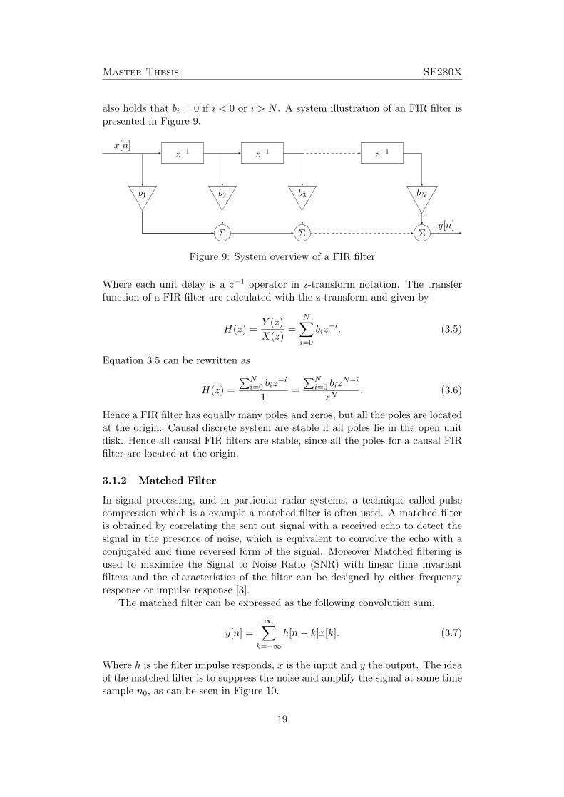
also holds that bi = 0 if i < 0 or i > N . A system illustration of an FIR filter ispresented in Figure 9.
b1
z−1
b2
Σ
z−1
b3
Σ
z−1
bN
Σ
x[n]
y[n]
Figure 9: System overview of a FIR filter
Where each unit delay is a z−1 operator in z-transform notation. The transferfunction of a FIR filter are calculated with the z-transform and given by
H(z) =Y (z)
X(z)=
N∑i=0
biz−i. (3.5)
Equation 3.5 can be rewritten as
H(z) =
∑Ni=0 biz
−i
1=
∑Ni=0 biz
N−i
zN. (3.6)
Hence a FIR filter has equally many poles and zeros, but all the poles are locatedat the origin. Causal discrete system are stable if all poles lie in the open unitdisk. Hence all causal FIR filters are stable, since all the poles for a causal FIRfilter are located at the origin.
3.1.2 Matched Filter
In signal processing, and in particular radar systems, a technique called pulsecompression which is a example a matched filter is often used. A matched filteris obtained by correlating the sent out signal with a received echo to detect thesignal in the presence of noise, which is equivalent to convolve the echo with aconjugated and time reversed form of the signal. Moreover Matched filtering isused to maximize the Signal to Noise Ratio (SNR) with linear time invariantfilters and the characteristics of the filter can be designed by either frequencyresponse or impulse response [3].
The matched filter can be expressed as the following convolution sum,
y[n] =
∞∑k=−∞
h[n− k]x[k]. (3.7)
Where h is the filter impulse responds, x is the input and y the output. The ideaof the matched filter is to suppress the noise and amplify the signal at some timesample n0, as can be seen in Figure 10.
19
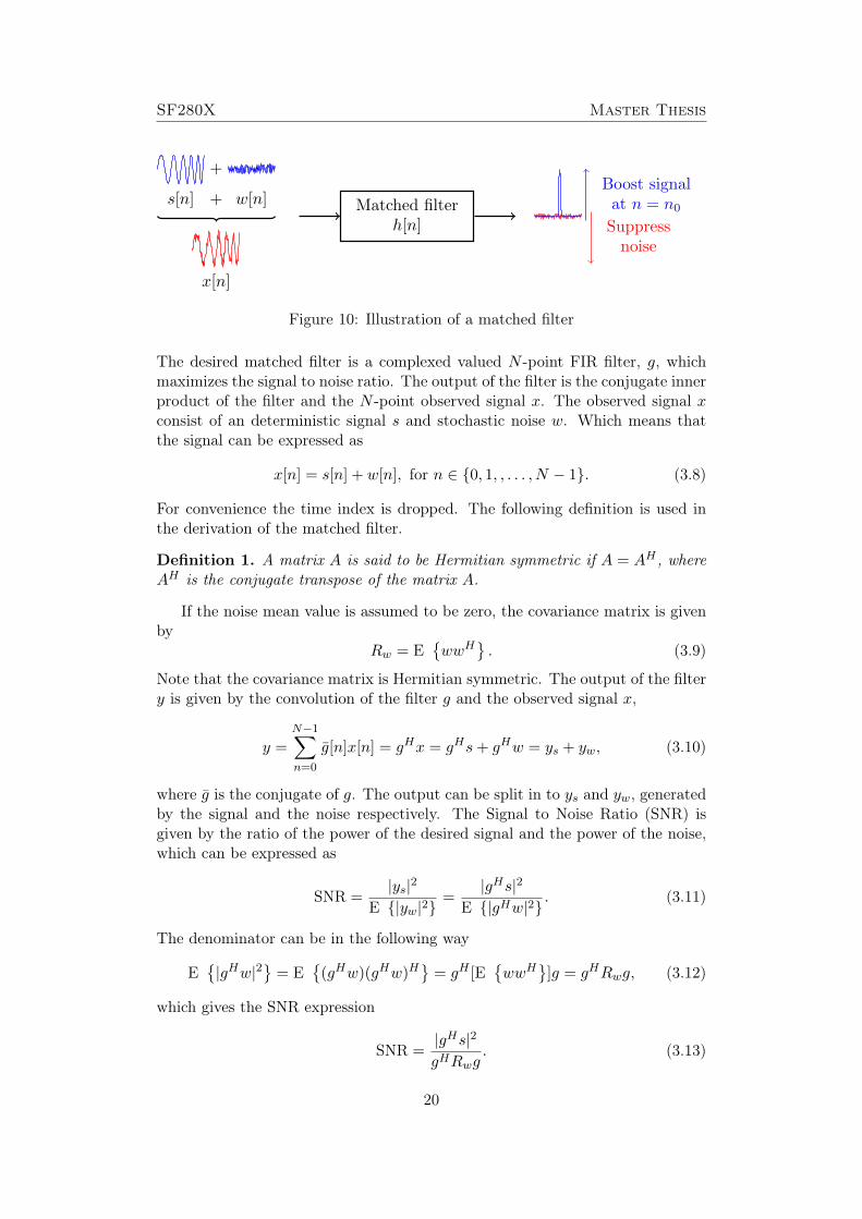
SF280X Master Thesis
Matched filterh[n]
+
s[n] + w[n]
x[n]
Suppressnoise
Boost signalat n = n0
Figure 10: Illustration of a matched filter
The desired matched filter is a complexed valued N -point FIR filter, g, whichmaximizes the signal to noise ratio. The output of the filter is the conjugate innerproduct of the filter and the N -point observed signal x. The observed signal xconsist of an deterministic signal s and stochastic noise w. Which means thatthe signal can be expressed as
x[n] = s[n] + w[n], for n ∈ {0, 1, , . . . , N − 1}. (3.8)
For convenience the time index is dropped. The following definition is used inthe derivation of the matched filter.
Definition 1. A matrix A is said to be Hermitian symmetric if A = AH , whereAH is the conjugate transpose of the matrix A.
If the noise mean value is assumed to be zero, the covariance matrix is givenby
Rw = E{wwH
}. (3.9)
Note that the covariance matrix is Hermitian symmetric. The output of the filtery is given by the convolution of the filter g and the observed signal x,
y =
N−1∑n=0
g[n]x[n] = gHx = gHs+ gHw = ys + yw, (3.10)
where g is the conjugate of g. The output can be split in to ys and yw, generatedby the signal and the noise respectively. The Signal to Noise Ratio (SNR) isgiven by the ratio of the power of the desired signal and the power of the noise,which can be expressed as
SNR =|ys|2
E {|yw|2}=
|gHs|2E {|gHw|2} . (3.11)
The denominator can be in the following way
E{|gHw|2
}= E
{(gHw)(gHw)H
}= gH [E
{wwH
}]g = gHRwg, (3.12)
which gives the SNR expression
SNR =|gHs|2gHRwg
. (3.13)
20
Master Thesis SF280X
Since the objective of the matched filter is to maximize the SNR, the problem isto solve the following optimization problem,
maxg
SNR (3.14)
or
maxg
|gHs|2gHRwg
. (3.15)
By using the property of Hermitian symmetry Equation 3.13 can be rewritten as
SNR =
∣∣∣∣gH(R12w)HR
− 12
w s
∣∣∣∣2gH(R
12w)HR
12wg
=
∣∣∣∣(gR 12w)H(R
− 12
w s)
∣∣∣∣2(gHR
12w)H(R
12wg)
. (3.16)
The Cauchy-Schwarz inequality is used to find an upper bound for the objectivefunction. For an complex inner product the Cauchy-Schwarz inequality is givenby
|uHv|2 ≤ ‖u‖2 · ‖v‖2 = (uHu) · (vHv), (3.17)the equality holds if and only if the vectors u and v are linear dependent. Hencean upper bound for the for the objective function is given by
SNR =
∣∣∣∣(gR 12w)H(R
− 12
w s)
∣∣∣∣2(gHR
12w)H(R
12wg)
≤
[(R
12wg)H(R
12wg)
] [(R− 1
2w s)H(R
− 12
w s)
](gHR
12w)H(R
12wg)
(3.18)
which simplifies toSNR ≤ sHR−1
w s. (3.19)The upper bound is achieved if and only if
R12wg = αR
− 12
w s, (3.20)
for an arbitrary scalar α. The optimal filer coefficients to the filter in Equation(3.10) can be expressed as
g = αR−1w s. (3.21)
If the noise is assumed to be zero mean withe noise (E yw = 0), the expectedvalue of the power can be expressed as the standard deviation of the noise σw,since
σw = E{|yw|2
}− (E {yw})2 = E
{|yw|2
}. (3.22)
The expectation value of the power of the noise can also be expressed as
E{|yw|2
}= E
{|gHw|2
}= (αR−1
w s)HRw(αR−1w s) = α2sHR−1
w s = σ2w (3.23)
givingα =
σw√sHR−1
w s. (3.24)
Which gives the normalized filter coefficients
g =σw√sHR−1
w sR−1w s. (3.25)
The matched filters impulse responds h is given by the complex conjugatetime reversal of g.
21

SF280X Master Thesis
3.2 Spectral Transforms
In order to be able so analyze frequency content of time signals the DiscreteFourier Transform (DFT) is introduced. This provide a method to analyze dis-crete signals since in real world applications continuous signals are rarely the casehence a method for managing discrete signals is needed.
3.2.1 Discrete Fourier Transform
If we start by the definition of complex Fourier series for a function x(t), t ∈{IR, 0 ≤ t ≤ T}
x(t) =∞∑
k=−∞cke
i2πnt/T
ck =1
T
∫ T
0x(t)e−ik2πt/Tdt.
(3.26)
Now instead of the continuous function x(t) consider discrete samples of x takenat time intervals δt. Introducing x[n] for the n:th sample of x(t) i.e. x(n∆t)of length N where N∆t = T . If now we calculate the Fourier coefficients ck inequation (3.26) as the sum over the samples x[n] instead of the integral
ck =1
T
N−1∑n=0
x[n]e−ik2πn∆t 1N∆t∆t
=1
N
N−1∑n=0
x[n]e−ik2πn 1N .
(3.27)
Where the right hand side of equation (3.27) is the definition of the DFT explicitlygiven by
X[k] =1
N
N−1∑n=0
x[n]e−ik2πnN . (3.28)
Corresponding to the DFT taking us from time domain to frequency domain theInverse Discrete Fourier Transform (IDFT) taking us the other way around isdefined by
x[n] =N−1∑k=0
X[k]eik2πnN . (3.29)
Note the scaling by 1/N in equation (3.28) and 1 in equation (3.29). It is quitecommon in literature to use the scaling the other way around, but as proposedhere the scaling is consistent with the Fourier series [5].A useful property of the DFT is the frequency shift property defined as
X[k − l] =1
N
N−1∑n=0
x[n]e−i2πnkN e
i2πnlN =
1
N
N−1∑n=0
x[n]e−i2πn(k−l)
N (3.30)
22

Master Thesis SF280X
that is in words by multiplying the discrete signal x[n] by the complex exponentialei2πnlN will generate a frequency shift in the spectrum with l.
3.3 Features
To be able to distinguish between various sound signals a set of latent variablesis needed, i.e. variables that are characteristic for the signal that can be used forcomparison without comparing the signal itself. The idea is as previously mentiona operator is listening to the sound signature of a target and as a compliment tothe human classification a feature driven classifier can act as support in situationswhen the operator is not certain on what kind of target is being listened to. Indigital speech processing a commonly used feature set are the Mel FrequencyCepstral Coefficients (MFCC) [22]. However the signal in this case are not aspeech signal and one can argue that it would not be a valid feature set forthis kind of classification. To motivate the choice of MFCC it have been shownthat using MFCC as a feature set for sound signal classification not being speechsignals. For example in [12] MFCC is used as features when classifying respiratorysounds signals and delivered satisfactory classification results. And in [8] MFCCare used and also compared to ordinary Cepstral Coefficients (CC) as a featureset for an classification of heart sound and in particular heart diseases, the resultshowed that MFCC was superior to CC in a classification task. The concept ofMFCC is to capture the human perceptual scale of frequencies, and incorporatingthis scale makes the features match more closely to what humans actually hear.To capture this a filter bank containing triangular filters evenly spaced in theMel scale is applied to the spectrum of the signal.
3.3.1 Mel Frequency Cepstral Coefficients
The MFCC feature extraction process used in this thesis is described belowLet x[n] be the discrete signal of length N , take the DFT of the signal
X[k] =
N−1∑n=0
x[n]e−i2nk/N 0 ≤ k < N. (3.31)
Construct a filter bank consisting ofM triangular filters ranging from frequenciesfstart to fmax given by
Hm[k] =
0 k < f(m− 1)k−f [m−1]
f [m]−f [m−1] f [m− 1] ≤ k ≤ [m]f [m+1]−k
f [m+1]−f [m] f [m] ≤ k ≤ f [m+ 1]
0 k > f [m+ 1]
(3.32)
the boundary points for the m:th filter is
f [m] =N
FsB−1
(B(fstart) +m
B(fmax)−B(fstart)
M + 1
). (3.33)
23

SF280X Master Thesis
Here Fs is the sampling frequency and B(f) is the mapping from physical fre-quency f to Mel scale
B(f) = 2595 log
(1 +
f
700
)(3.34)
and thus
B(b)−1(b) = 700(eb/2595 − 1). (3.35)An example of a such filter bank is illustrated in Figure 11. The filter bank is beuniformly spaced in the Mel scale and consequently the bandwidth of each filterwill increase logarithmically in the normal scale.
Figure 11: Illustration of a Mel filter bank withM = 10, fstart = 0, fmax = 4000
The energy in each band (m:th filter) is computed as
S[m] = log
(N−1∑k=0
|X[k]|2Hm[k]
)0 < m ≤M. (3.36)
The resulting S[m], is a representation of the energies that is sensitive in a wayhuman hearing works in terms of frequencies.
The final step to extract the MFCC is to apply the Discrete Cosine Transformto the filter bank energies
c[n] =M−1∑m=0
S[m] cos
(πn(m− 0.5)
M
)0 < n ≤M. (3.37)
24
Master Thesis SF280X
Where c[n] are the MFCC, typically 8-13 coefficients are used when used as afeature set for classification [15] with a filter bank consisting of 26-40 filters.
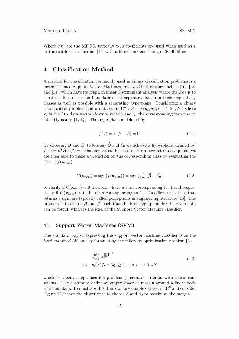
4 Classification Method
A method for classification commonly used in binary classification problems is amethod named Support Vector Machines, reviewed in literature such as [16], [23]and [11], which have its origin in linear discriminant analysis where the idea is toconstruct linear decision boundaries that separates data into their respectivelyclasses as well as possible with a separating hyperplane. Considering a binaryclassification problem and a dataset in IRn : S = {(xi, yi); i = 1, 2.., N} wherexi is the i:th data vector (feature vector) and yi the corresponding response orlabel (typically {1,-1}). The hyperplane is defined by
f(x) = xTβ + β0 = 0. (4.1)
By choosing β and β0 to lets say β and β0 we achieve a hyperplane, defined by,f(x) = xT β+ β0 = 0 that separates the classes. For a new set of data points weare then able to make a prediction on the corresponding class by evaluating thesign of f(xnew),
G(xnew) = sign(f(xnew)) = sign(xTnewβ + β0) (4.2)
to clarify if G(xnew) < 0 then xnew have a class corresponding to -1 and respec-tively if G(xnew) > 0 the class corresponding to 1. Classifiers such this, thatreturns a sign, are typically called perceptions in engineering literature [16]. Theproblem is to choose β and β0 such that the best hyperplane for the given datacan be found, which is the idea of the Support Vector Machine classifier.
4.1 Support Vector Machines (SVM)
The standard way of expressing the support vector machine classifier is as thehard margin SVM and by formulating the following optimization problem [23]
minβ,β0
1
2||β||2
s.t yi(xTi β + β0) ≥ 1 for i = 1, 2...N
(4.3)
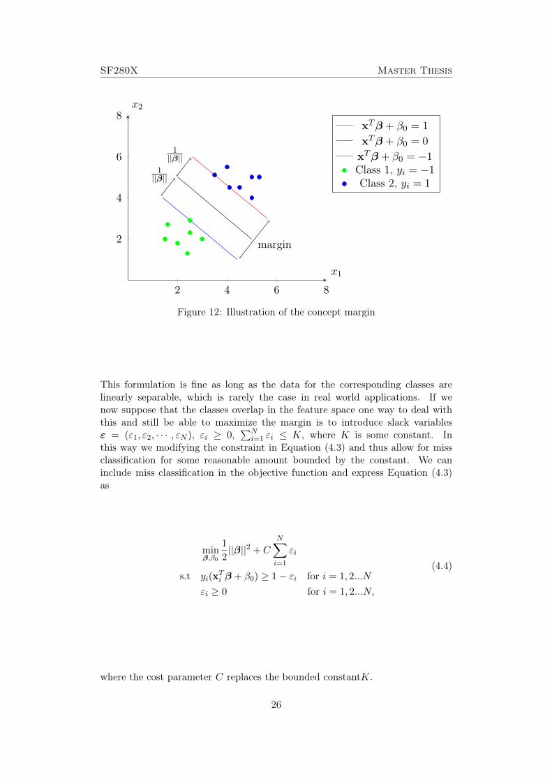
which is a convex optimization problem (quadratic criterion with linear con-strains). The constrains define an empty space or margin around a linear deci-sion boundary. To illustrate this, think of an example dataset in IR2 and considerFigure 12, hence the objective is to choose β and β0 to maximize the margin.
25
SF280X Master Thesis
2 4 6 8
2
4
6
8
margin
1||β||
1||β||
x1
x2
xTβ + β0 = 1
xTβ + β0 = 0
xTβ + β0 = −1Class 1, yi = −1Class 2, yi = 1
Figure 12: Illustration of the concept margin
This formulation is fine as long as the data for the corresponding classes arelinearly separable, which is rarely the case in real world applications. If wenow suppose that the classes overlap in the feature space one way to deal withthis and still be able to maximize the margin is to introduce slack variablesε = (ε1, ε2, · · · , εN ), εi ≥ 0,
∑Ni=1 εi ≤ K, where K is some constant. In
this way we modifying the constraint in Equation (4.3) and thus allow for missclassification for some reasonable amount bounded by the constant. We caninclude miss classification in the objective function and express Equation (4.3)as
minβ,β0
1
2||β||2 + C
N∑i=1
εi
s.t yi(xTi β + β0) ≥ 1− εi for i = 1, 2...N
εi ≥ 0 for i = 1, 2...N,
(4.4)
where the cost parameter C replaces the bounded constantK.
26

Master Thesis SF280X
2 4 6 8
2
4
6
8
ε1
ε2
ε3
margin
1||β||
1||β||
x1
x2
xTβ + β0 = 1
xTβ + β0 = 0
xTβ + β0 = −1Class 1, yi = −1Class 2, yi = 1
Figure 13: Illustration of the introduction of slack variables εi which allow formiss classification
Figure 13 illustrates this concept, points on the margin will have εi = 0 andpoints inside (or even pass the separating hyperplane) will have ε > 0
4.2 Dual Formulation
By formalizing Equation (4.4) as its dual formulation will result in a simpler con-vex quadratic optimization problem and can be solved with standard techniques[16], but the main benefit is that it will be possible to to express the problem interms of dot products of vectors in the feature space xTi xj , further more this willbe the key concepts when, explaned further down, specify a non linear transfor-mation of the feature vectors allowing for non linear decision boundraries andtake use of the Kernel Trick. A note on Lagrangian duality in correspondence tothe SVM can be found in [11]. The Lagrangian primal function is
Lp =1
2||β||2 + C
N∑i=1
εi −N∑i=1
αi[yi(xTi β + β0)− (1− εi)
]−
N∑i=1
µiεi (4.5)
where αi ≥ 0, µi ≥ 0 are the Lagrange multipliers and Lp is to be minimizedwith respect to β, β0 and εi. Setting the derivatives to zero we achieve
β =
N∑i=0
αiyixi
N∑i=1
αiyi = 0
αi = C − µi ∀i.
(4.6)
27
SF280X Master Thesis
Inserting the Equations in (4.6) in Equation (4.5) and simplifying we obtain thefollowing dual form
maxα
N∑i=1
αi −1
2
N∑i=1
N∑j=1
αiαjyiyjxTi xj
s.t 0 ≤ αi ≤ C ∀iN∑i=1
αiyi = 0.
(4.7)
In addition to the Equations in (4.6), the Karush-Kuhn-Tucker conditions includethe constraints
αi(yi(xTi β + β0)− (1− εi)) = 0
µiεi = 0
(yi(xTi β + β0)− (1− εi)) ≥ 0.
(4.8)
After solving the dual problem we need to obtain the primal solution to classifynew points i.e. we need β and β0, inspecting the first Equation in (4.6) we noticethat the solution for β is on the form
β =
N∑i=1
αiyixi (4.9)
which includes the Lagrange multipliers αi with the corresponding i:th obser-vation. These observations are, in literature, denoted as the support vectors orsupport points. As can be seen in Figure 13 points on the boundary will haveεi = 0 which corresponds to 0 < αi < C which follows by the second Equationin (4.8) and the last Equation in (4.6). Hence the first Equation in (4.8) can beused to solve β0.
The decision function for classifying new inputs is now
f(xnew) = xTnewβ + β0 =
N∑i=1
αiyixTnewxi + β0 (4.10)
and by investigating the sign of the above the class can be determined as ex-plained in Equation (4.2).
4.3 Kernel Trick
SVM:s are, as mentioned, a linear classifier and to improve classification onewould like to relax this condition in a way not only being capable to handleoverlapping data sets with the method of introduce slack described above. Ratherthan using our original features x we may want to learn some features φ(x) [11]
This process consist of two steps, first the input vectors are transformed, ormapped, to some high dimensional feature vectors by the mapping φ, then theSVM finds the hyperplane that maximizes the margin in the new feature space.
28
Master Thesis SF280X
The separating hyperplane will be a linear function in the transformed but a nonlinear in the original feature space.
Consider the optimization problem in (4.7) and an optional transformationφ(·) of the input data
maxα
N∑i=1
αi −1
2
N∑i=1
N∑j=1
αiαjyiyjφ(xi)Tφ(xj)
s.t 0 ≤ αi ≤ C ∀iN∑i=1
αiyi = 0.
(4.11)
and the solution function, Equation (4.10) yields
f(xnew) =N∑i=1
αiyiφ(xnew)Tφ(xi) + β0 (4.12)
In both Equation (6.1) and (4.12) we see that the objective function and thesolution function includes the transformation φ(·) in terms of dot products ofthe transformed feature vectors. Instead of explicitly define the transformationφ(·), which can lead to very high dimensional feature vectors in the transformedfeature space, one can instead make use of the Kernel trick which returns the dotproduct directly computed in the original feature space.
Now given the feature mapping φ(·) we define the corresponding Kernel tobe
K(xi,xj) = φ(xi)Tφ(xj). (4.13)
Instead of explicitly find or represent φ(xi) and φ(xj) we can directly define theKernel in terms of xi and xj by some Kernel function.
Popular Kernels to use are in SVM literature [16],
• K(xi,xj) = (1 + xTi xj)p, p-Degree polynomial Kernel,
• K(xi,xj) = e−||xi−xj ||
2
2σ2 , Radial basis or Gaussian Kernel,
• K(xi,xj) = tanh(κ1xTi xj + κ2) , Sigmoid Kernel.
with corresponding parameters p, σ,κ1 and κ2 to choose for the model. In generalthe Radial basis kernel is a reasonable first choice since it has fewer numericaldifficulties and the Sigmoid Kernel is not valid under some parameters κ1 and κ2
[6].
29

SF280X Master Thesis
5 Radar Signal Processing
When the radar system send out electromagnetic signals st(t) in the free spaceand receive echoes sr(t) from the surrounding environment. The received echoesare transformed with an quadrature detector to an I/Q signal sD who is rep-resented in the free space as x[n,m] where n represents the shift in bearing asthe radar revolves and m represents a range. Much of the returned signals isfrom objects of non interest such as buildings, threes and even the ground itself.Echoes from these kinds of objects are often called ground clutter or clutter. Dueto the presence of clutter, further signal processing is needed on the raw radarvideo before extracting the radar echoes (I/Q data) from targets, since clutterechoes can be many orders of magnitude larger than the target itself. This can beseen in Figure 14 where the instantaneous power of x[n,m] is plotted in decibel
Pinst = 20 log10 |x[n,m]|. (5.1)
The plot it hardly dominated by clutter and it is impossible to resolve echoesfrom targets. To be able to resolve targets and extract I/Q data from a targettwo signals processing methods are used, MTI-filtering and pulse compression.Echoes from targets can then be extracted as complex time series, by taking theFourier Transform of these signals the Doppler spectrum are achieved.
Figure 14: Raw radar video
30

Master Thesis SF280X
5.1 MTI-filter
The Moving Target Indicator (MTI) filter is used to suppress echoes from clutter,a property of clutter is that it is stationary or close to stationary, i.e., the Dopplerfrequencies induced by echoes from clutter is zero or close to zero. The MTI filteris a high pass filter that filters out the low Doppler frequencies, i.e. the objectswith low velocities. The MTI filters used are FIR filters of order N (numberof filter coefficients) explained in section 3.1.1 and for a set of impulse responsecoefficients bi and the signal x[n,m] the filtered signal xmti[n,m] can be expressedas the following convolution sum
xmti[n,m] =N∑i=0
bix[n− i,m], for all m, (5.2)
A graphical representation of the instantaneous power of the MTI filtered signalearlier seen in Figure 14 as its raw form can be seen in Figure 15.
Figure 15: MTI filtered radar video
As can be seen in Figure 15 most of the clutter is removed and it is possible todistinguish echoes returned from targets.
31
SF280X Master Thesis
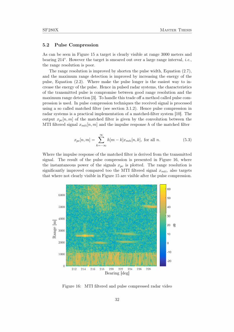
5.2 Pulse Compression
As can be seen in Figure 15 a target is clearly visible at range 3000 meters andbearing 214◦. However the target is smeared out over a large range interval, i.e.,the range resolution is poor.
The range resolution is improved by shorten the pulse width, Equation (2.7),and the maximum range detection is improved by increasing the energy of thepulse, Equation (2.2). Where make the pulse longer is the easiest way to in-crease the energy of the pulse. Hence in pulsed radar systems, the characteristicsof the transmitted pulse is compromise between good range resolution and themaximum range detection [3]. To handle this trade off a method called pulse com-pression is used. In pulse compression techniques the received signal is processedusing a so called matched filter (see section 3.1.2). Hence pulse compression inradar systems is a practical implementation of a matched-filter system [10]. Theoutput xpc[n,m] of the matched filter is given by the convolution between theMTI filtered signal xmti[n,m] and the impulse response h of the matched filter
xpc[n,m] =∞∑
k=−∞h[m− k]xmti[n, k], for all n. (5.3)
Where the impulse response of the matched filter is derived from the transmittedsignal. The result of the pulse compression is presented in Figure 16, wherethe instantaneous power of the signals xpc is plotted. The range resolution issignificantly improved compared too the MTI filtered signal xmti, also targetsthat where not clearly visible in Figure 15 are visible after the pulse compression.
Ran
ge[m
]
Bearing [deg]
Figure 16: MTI filtered and pulse compressed radar video
32
Master Thesis SF280X
5.3 Signal Extraction
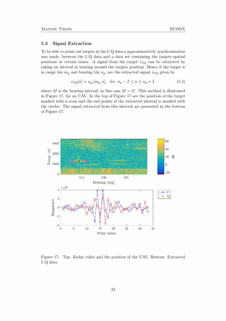
To be able to point out targets in the I/Q data a approximatively synchronizationwas made, between the I/Q data and a data set containing the targets spatialpositions at certain times. A signal from the target xIQ can be extracted bytaking an interval in bearing around the targets position. Hence if the target isin range bin mp and bearing bin np, are the extracted signal xIQ given by
xIQ[n] = xpc[mp, n], for np − I ≤ n ≤ np + I, (5.4)
where 2I is the bearing interval, in this case 2I = 3◦. This method is illustratedin Figure 17, for an UAV. In the top of Figure 17 are the position of the targetmarked with a cross and the end points of the extracted interval is marked withthe circles. The signal extracted from this interval are presented in the bottomof Figure 17.
Figure 17: Top: Radar video and the position of the UAV. Bottom: ExtractedI/Q data
33
SF280X Master Thesis
5.4 Spectral Modifications
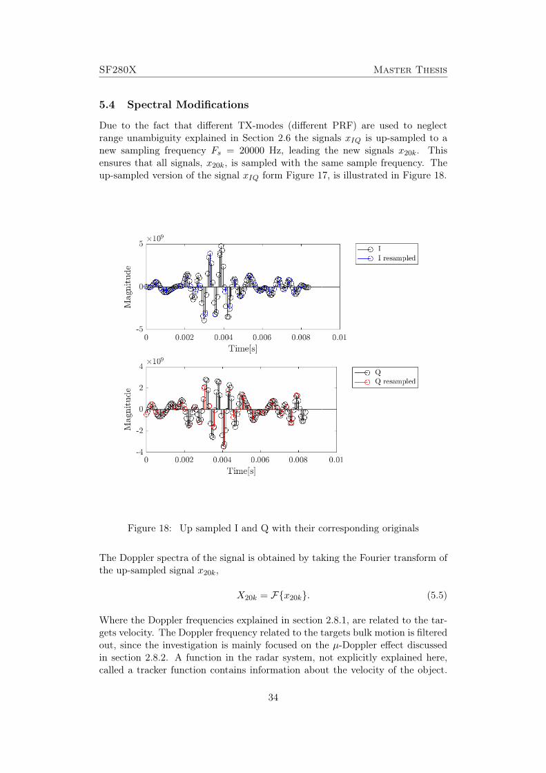
Due to the fact that different TX-modes (different PRF) are used to neglectrange unambiguity explained in Section 2.6 the signals xIQ is up-sampled to anew sampling frequency Fs = 20000 Hz, leading the new signals x20k. Thisensures that all signals, x20k, is sampled with the same sample frequency. Theup-sampled version of the signal xIQ form Figure 17, is illustrated in Figure 18.
Figure 18: Up sampled I and Q with their corresponding originals
The Doppler spectra of the signal is obtained by taking the Fourier transform ofthe up-sampled signal x20k,
X20k = F{x20k}. (5.5)
Where the Doppler frequencies explained in section 2.8.1, are related to the tar-gets velocity. The Doppler frequency related to the targets bulk motion is filteredout, since the investigation is mainly focused on the µ-Doppler effect discussedin section 2.8.2. A function in the radar system, not explicitly explained here,called a tracker function contains information about the velocity of the object.
34

Master Thesis SF280X
The targets velocity can be represented as a Doppler frequency, by Equation(2.14).
The filtering is made by shifting the spectra using the frequency shift propertyof the DFT described in Section 3.2.1. The Doppler frequency that correspondsto the current velocity of the object is shifted to DC (frequency = 0), by
Xshift[k] = X20k[k − l], (5.6)
where l is the frequency shift. The spectral content at the DC frequency in theshifted spectra is filtered out with a FIR filter, described in Section 3.1.1. Givingthe spectra of the shifted and filtered signal Xshift,F IR[k]. The spectra is shiftedback with the same frequency shift property of the DFT, crating the filteredsignal,
XFIR[k] = Xshift,F IR[k + l], (5.7)
where l is the same frequency shift. The process is graphically illustrated inFigure 19 below.
Figure 19: Top: Original spectrum and velocity corresponding to the target.Middle: Shifted spectrum and filtered spectrum with a FIR filter. Bottom:Spectrums shifted to the original position
35

SF280X Master Thesis
The signal that generates the Doppler spectrum is complex and to be able to aextract a real signal from the Doppler spectrum the spectrum need to be symmet-ric. In this thesis the method to achieve a real signal that have some correlationin a meaningful way is to use shift the whole spectrum by the frequency shiftproperty of the DFT and then mirror the spectrum, denoted Xmirror, illustratedin Figure 20.
Figure 20: Top: Original spectrum Middle: Shifted spectrum Bottom: Mirroredspectrum
By then taking the Inverse Fourier Transform it is possible to extract a realsignal, denoted xreal.
xreal = F−1{Xmirror} (5.8)
It should also be noted that depending on the sign on the velocity (moving fromor towards the radar) i.e., the sign on the Doppler frequency corresponding tothe velocity the spectrum is shifted to right or left to not let the direction ofmovement induce characteristics on the two objects.
36

Master Thesis SF280X
6 Data Sets and Implementation
The signals, xreal, resulting from section 5 are transformed to signals, xaudio,that are audible and could be listen to by an operator. In complement to thehuman perception a machine driven data classification is needed to support theoperator when not being able to distinguish these signals for various reasons.To be able to do this, characteristics for the signals is needed commonly knownas features. In this thesis a feature set commonly used in speech processing isused, namely Mel Frequency Cepstral Coefficients (see Section 3.3). This featureset will be used as input for a feature driven classification method who thencan be used to predict and classify new input data. The classification methodused is called Support Vector Machine (SVM) who have its origin in LinearDiscriminant Analysis (see Section 4). The idea of the SVM method formulatingthe discrimination problem as a optimization problem where the aim is to find thebest separating discriminator in the feature space. Moreover, a dual formulationof the optimization problem will provide more flexibility of the SVM methodsince it allow us to use the Kernel Trick and thus achieve the non linear SVMmethod. The classification method training phase includes a set of parametersdepending on how you model with respect to the data, these parameters arechosen with a method called cross validation in the implementation, finally theclassifier is tested on the ability to classify input data.
6.1 Data Set
The dataset originated from the signal processed radar echoes of UAV:s andbirds as the results described in section 5 is transformed to signals that would beaudible, and thus possible for an radar operator to listen to, explicitly describedin the thesis of Johan Clemedson [2], with the idea that by human perception aradar operator would be able to classify these sounds. In short the signals xrealare extrapolated with an AR-filter with Burg’s method. This is done, withoutgoing in on details, by estimating so called AR parameters from the xreal signals.For each signal an AR-filter of order 40 is estimated with Burg’s method. Eachsignal xreal is then extrapolated using the AR-filter and presented as an audiooutput xaudio. The data set consist of 181 audio signals related to radar echoesfrom a UAV and 232 audio signals related to birds. This data set consisting of413 audio signals in total will will serve as basis for the development of a featuredriven classifier.
6.2 Implementation
MFCC Features from the signals, xaudio, where extracted as described in sec-tion 3.3.1 to represent the characteristics of each class, with 40 filters and thefirst 13 MFCC each signal where represented as a 13-dimensional vector ci forthe i:th signal. The implementation of a SVM classifier model, defined by theoptimization problem
37

SF280X Master Thesis
maxα
N∑i=1
αi −1
2
N∑i=1
N∑j=1
αiαjyiyjφ(ci)Tφ(cj)
s.t 0 ≤ αi ≤ C ∀iN∑i=1
αiyi = 0,
(6.1)
is made in MATLAB and in particular with the Statistics and Machine Learningtoolbox which allow modeling with the linear kernel (no transformation φ of thefeature vector) and the radial basis kernel which corresponds to a non lineartransformation φ in the sense
φ(ci)Tφ(cj) = e−||ci−cj ||
2
2σ2 . (6.2)
The analysis is performed on a so called linear model (linear kernel), and a trans-formation related to the radial basis kernel with the corresponding parametersC and (C, σ) respectively to be tuned for both models. To train, tune and testthe models the following approach is used.
• Split data into a training and testing set– The total set of available signals containing of 413 signals, hence 413MFCC feature vectors. 30 signals of each class is used for validation ofthe models and the remaining 353 to build the model.
• Consider the linear and radial basis model– The linear model consist of the parameter C to be determined. The ra-dial basis model have, beyond C, a parameter from the kernel function,hence σ also needs to be determined.
• Use Cross-validation to find best parameters for the models– By splitting the training data in folds (subsets) to measure the predic-tion error and sequentially swap these folds in terms of what folds areused for training and testing and then take the average of these sequen-tially measured prediction error a more generalized parameter selectionare achieved that takes the whole data set in account i.e. not just onesubset are used for testing.
• Use the best parameters to train the models– The best parameters (who gives lowest prediction error) are used to trainthe models.
• Test the models– The models are tested with the 60 signals that are not used in thetraining phase and hence the 60 signals can be seen as new observationsand serves as a final validation on how good the models are to predictnew data.
38

Master Thesis SF280X
6.3 Training and Parameter Evaluation
Two classification models where trained, the SVM without any transformation ofthe features (linear) and the SVM with the radial basis kernel. The first modelsonly consist of the cost parameter for miss classification C and the radial basismodel also have the scale parameter σ.
The performance of the of the models can be represented by a confusionmatrix which contains information of how well the model performed on data youfeed to the model, known as the test data. An illustration of such a representationcan be seen in Table 1.
PredictedInput Class 1 Class 2Class 1 P11 P12
Class 2 P21 P22
• Pii : Number of occurrences of Class i that is predicted as Class i
• Pij : Number of occurrences of Class i that is predicted as Class j, i 6= j
Table 1: Illustration of a confusion matrix for the two class problem
By examine the the confusion matrix one will get an idea of how good the modelpredicted on the test data. The diagonal values in the confusion matrix contains"overall" information of how good the model is to predict new data, but usefulinformation can also be gathered to examine off diagonal values, for example tofind out if a model predicting a specific class better than other classes.To adjust model parameters the prediction error of the model is used, whichsimply are the number of wrongly classified observations in the test set dividedby the total number of observations in the test set. The approach is simplyto test parameters C and (C, σ) for the respective models and then use thoseparameters when evaluating future performance of the classification models. Inrelation to Table 1 the prediction error is defined as
prediction error =P12 + P21
N, (6.3)
where N is the size of the test set.To improve parameter selection a cross validation approach is used. This meansthat you instead of test and evaluate the prediction error your model with asingle test set the test data is partitioned in M subsets or folds. Moreover thetraining part now consist of M − 1 of these folds and 1 fold used for evaluationof the prediction error, now one iteration or trail has been completed. The nextstep is to useM −1 new folds for the training part and 1 new fold for evaluation.After completed M trails in this process the average of the prediction error isused to chose model parameters in the sense that parameters that generate alow average prediction error will be result in the model that best fits the data
39

SF280X Master Thesis
with the "whole" data set in mind. An illustration of the cross validation schemewhere M = 5 can be seen in Figure 21 below.
data set
class 1 (UAV) class 2 (Bird)
fold
1fold
2fold
3fold
4fold
5
fold
1fold
2fold
3fold
4fold
5
training set
testing set
trail 1 error 1trail 2 error 2trail 3 error 3trail 4 error 4trail 5 error 5
Average Overall error
Figure 21: Illustration of cross validation scheme
40

Master Thesis SF280X
7 Results
The linear model where tested for the parameter C in the interval [1, 100] consist-ing of 10 logarithmically equal spaced values for C. The cross validated modelsoverall test error, explained in Section 6.3 where the training data set where splitin 5 folds and the prediction error was measured by Equation (6.3) and hencethe overall test error is the average of these 5 prediction errors, was evaluated fordifferent values of C. The resulting test error is illustrated in Figure 22.
0 0.2 0.4 0.6 0.8 1 1.2 1.4 1.6 1.8 2log(C)
0.055
0.06
0.065
0.07
0.075
erro
r
0 0.2 0.4 0.6 0.8 1 1.2 1.4 1.6 1.8 2log(C)
0
0.02
0.04
0.06
erro
r
Figure 22: Test error of linear model for various values on the parameter C
As can be seen the model is not particular sensitive for the parameter C, since thetest error do not change significantly while varying the parameter C which is moreclear when inspecting the lower plot on Figure 22. However the best parametervalue, who gives the lowest test error C corresponds to log(C) = 0.4444.
The same approach where implemented for the radial basis (RB) model with theparameter pair (C, σ), also here the test values for the parameter σ in the interval[1, 100] consisting of 10 logarithmically equal spaced test parameters, illustratedin Figure 23
41

SF280X Master Thesis
Figure 23: Test error of radial basis model for various parameters (C, σ)
As can be seen the test error does not change significantly for a large range ofparameter values. To further compare the two models, for a set of σ values thetest error depending on C is plotted for the radial basis model together with thelinear model in Figure 24.
42
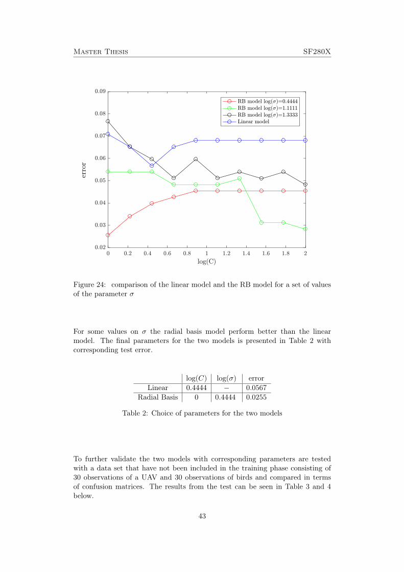
Master Thesis SF280X
error
Figure 24: comparison of the linear model and the RB model for a set of valuesof the parameter σ
For some values on σ the radial basis model perform better than the linearmodel. The final parameters for the two models is presented in Table 2 withcorresponding test error.
log(C) log(σ) errorLinear 0.4444 − 0.0567
Radial Basis 0 0.4444 0.0255
Table 2: Choice of parameters for the two models
To further validate the two models with corresponding parameters are testedwith a data set that have not been included in the training phase consisting of30 observations of a UAV and 30 observations of birds and compared in termsof confusion matrices. The results from the test can be seen in Table 3 and 4below.
43

SF280X Master Thesis
PredictedInput UAV BIRDUAV 28 2
BIRD 2 28
Table 3: Test performance linear model
PredictedInput UAV BIRDUAV 30 0
BIRD 1 29
Table 4: Test performance RB model
In general the radial basis model perform better than the linear model, both interms of test error in the training phase where the radial basis model achieved atest error of 2.55% compared to the linear model with a test error of 5.67%. Alsoin when the models where compared with a independent test set the radial basisperformed better with 100.00% correct prediction on the UAV and 96.67% onbirds compared to the linear model with 93.33% correct prediction on the UAVand 93.33% on birds. Overall the final models predicted correct on 98.33% and93.33% with the radial basis model and the linear model respectively.
44

Master Thesis SF280X
8 Discussion and Future Work
In this project a method for extracting radar returns from raw radar data havebeen proposed in combination with an aurial output, explicitly explained in thethesis of Johan Clemedson [2], a feature driven classification method with MFCCas a descriptor for these signals and a Support Vector Machine as classificationmethod have also been implemented. There have been many moving pars throughout this project, data processing, signal processing, machine learning and by this,a small change in the beginning of the process can change a lot further down theroad which have made this project to an iterative and changing process.
The project was heavily dependent on the data available and since most ofthe data was poor and even bad as illustrated in in Figure 25 and 26. A reason forthis may be that the field test when gartering data, many radar systems whereused at the same time and hence this could be interferences due to this cause.
Figure 25: Illustration 1 of interference in the available data
Figure 26: Illustration 2 of interference in the available data
45
SF280X Master Thesis
It was hard to find good methods to come up with a purposed solution andmany ideas have been purposed but later discarded. Indeed, the available dataset was small but methods that works for this data set was developed. In futurework more data have to be gathered to validate this methods before a real timeimplementation can be done.
The data from the UAV consist of only one type of UAV, more data is neededto investigate how these methods will perform when there are different typesof UAV:s to discriminate between. One possibility is that this kind of UAVexamined in the project implies such discrimination in the radar returns that itis possible to use these methods to distinguish between this UAV and birds butwill fail when include others kinds of UAV:s in the analysis.
The feature set used in this thesis has its origin in speech processing, differentways of implementing this can be used but the purposed method in this thesisseems to work good for this kind of problem setup. In further analysis oneshould investigate other feature set that have the possibility to serve as input toa classification method and provide perhaps even better results. Further moreon this theme, one may want to use another kind of classification method moreadapted to aural classification for example Hidden Markov Models that are usedin speech processing.
The grid search method for finding good parameters for respective SVMmodel are time consuming, but in this case when having a small amount ofdata it is affordable. However if more data is gathered it is not sure that theparameters used in this thesis will be the best for the new data set and it isrecommended to re do the grid search or use another method to determine theparameters. One could also use a finer grid, or even a completely different spac-ing, than the grid used to see if it is possible to achieve even lower classificationerror, however this is not done in this thesis due to the fact that the results aresatisfactory.
To summarize, this project can be seen to serve as a pilot for future work in anew way in the area of radar classification, ideas, methods and thoughts on howto attack a problem like this.
46
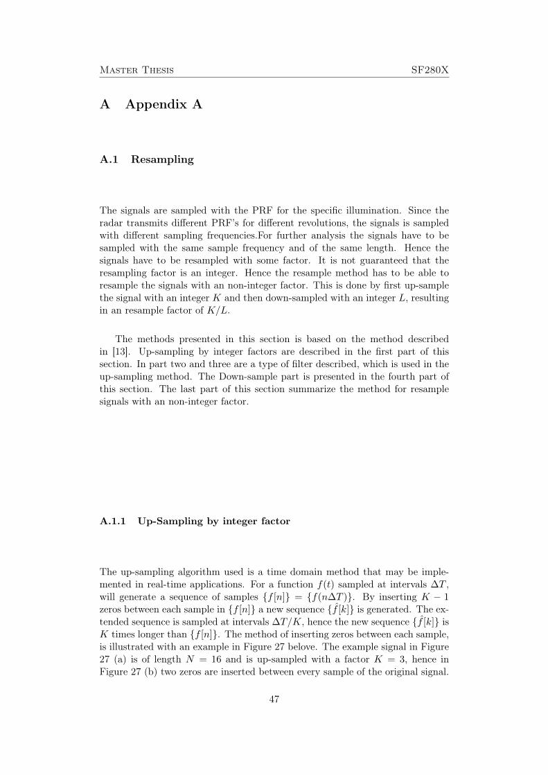
Master Thesis SF280X
A Appendix A
A.1 Resampling
The signals are sampled with the PRF for the specific illumination. Since theradar transmits different PRF’s for different revolutions, the signals is sampledwith different sampling frequencies.For further analysis the signals have to besampled with the same sample frequency and of the same length. Hence thesignals have to be resampled with some factor. It is not guaranteed that theresampling factor is an integer. Hence the resample method has to be able toresample the signals with an non-integer factor. This is done by first up-samplethe signal with an integer K and then down-sampled with an integer L, resultingin an resample factor of K/L.
The methods presented in this section is based on the method describedin [13]. Up-sampling by integer factors are described in the first part of thissection. In part two and three are a type of filter described, which is used in theup-sampling method. The Down-sample part is presented in the fourth part ofthis section. The last part of this section summarize the method for resamplesignals with an non-integer factor.
A.1.1 Up-Sampling by integer factor
The up-sampling algorithm used is a time domain method that may be imple-mented in real-time applications. For a function f(t) sampled at intervals ∆T ,will generate a sequence of samples {f [n]} = {f(n∆T )}. By inserting K − 1zeros between each sample in {f [n]} a new sequence {f [k]} is generated. The ex-tended sequence is sampled at intervals ∆T/K, hence the new sequence {f [k]} isK times longer than {f [n]}. The method of inserting zeros between each sample,is illustrated with an example in Figure 27 belove. The example signal in Figure27 (a) is of length N = 16 and is up-sampled with a factor K = 3, hence inFigure 27 (b) two zeros are inserted between every sample of the original signal.
47
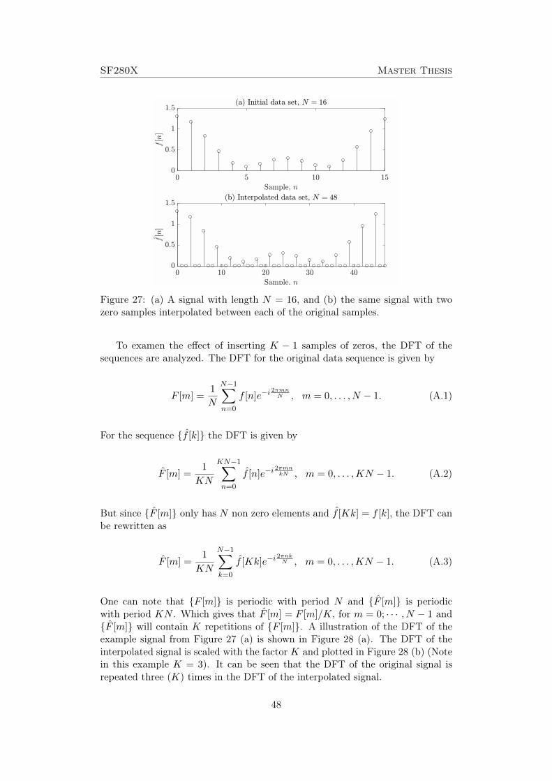
SF280X Master Thesis
Figure 27: (a) A signal with length N = 16, and (b) the same signal with twozero samples interpolated between each of the original samples.
To examen the effect of inserting K − 1 samples of zeros, the DFT of thesequences are analyzed. The DFT for the original data sequence is given by
F [m] =1
N
N−1∑n=0
f [n]e−i2πmnN , m = 0, . . . , N − 1. (A.1)
For the sequence {f [k]} the DFT is given by
F [m] =1
KN
KN−1∑n=0
f [n]e−i2πmnkN , m = 0, . . . ,KN − 1. (A.2)
But since {F [m]} only has N non zero elements and f [Kk] = f [k], the DFT canbe rewritten as
F [m] =1
KN
N−1∑k=0
f [Kk]e−i2πnkN , m = 0, . . . ,KN − 1. (A.3)
One can note that {F [m]} is periodic with period N and {F [m]} is periodicwith period KN . Which gives that F [m] = F [m]/K, for m = 0; · · · , N − 1 and{F [m]} will contain K repetitions of {F [m]}. A illustration of the DFT of theexample signal from Figure 27 (a) is shown in Figure 28 (a). The DFT of theinterpolated signal is scaled with the factor K and plotted in Figure 28 (b) (Notein this example K = 3). It can be seen that the DFT of the original signal isrepeated three (K) times in the DFT of the interpolated signal.
48

Master Thesis SF280X
Figure 28: DFT of the signal shown in 27 (a), which is periodic with period 16.DFT of the interpolated signal shown in 27 (b), which is periodic with period 48.
By insertingK−1 zeros has resulted in a signal with sampling interval ∆T/Kand a Nyquist frequency of K/(2∆T ). The frequency resolution is unchangedand the original DFT is replicated K times within the frequency span of K/∆T .The interpolated signal can be reconstructed by elimination of the replicationsof the original spectral components. This is done by applying a low-pass filterto the sequence {F [m]} to preserve only the base band part of the spectrum.A representation of the two sided spectrum of f [m] are presented in Figure 29.Which illustrates the replications of F [m] and the low-pass filtering process.
mf
F [m]
−KN/2f = −K/(2∆T )
KN/2f = K/(2∆T )
0
Replications of F [m]
Passband oflow-pass filter
Low-passfilter
mf
F [m]
−KN/2f = −K/(2∆T )
KN/2f = K/(2∆T )
0
Nyquistfrequency
Figure 29: Illustration of low-pass filtering used to eliminate spectral replicationsintroduced by the interpolation of the signal.
49

SF280X Master Thesis
The algorithm used to upsample a signal with an integer factor K can besummarized in the block diagram, displayed in Figure 30.
Insert K − 1 zerosbetween samples
Low-passfilter
f [n] f [n] Interpolated waveform
t t t∆T ∆T
K
Figure 30: Block diagram of the algorithm for upsample a sequence with aninteger factor K.
The interpolation filter used as the low-pass filter in the upsample algorithm isdescribed in the next section.
A.1.2 Interpolation Filter
The ideal filter for the interpolated sequence, is a low pass filter with cut offfrequency at the Nyquist frequency of the original signal 1/(2∆T ). The impulseresponse of such a filter is given by
h[n] =sin(πn/K)
πn/K(A.4)
But this kind of filters are acausal, hence a FIR approximation is made. Thisis done by truncating h[n] to a finite length. If one sets the finite length toN = 2KM + 1 and delaying it with KN samples the FIR approximation isobtained as
h[n] =sin(π(n−KM)/K)
π(n−KM)/K, n = 0; . . . , N − 1. (A.5)
The resampled signal is also windowed by a Kaiser window in the filtering process.The Kaiser window is explained in more detail in Section A.1.6.
The FIR interpolation filter for a up-sample factor K is illustrated in Figure31, below.
Up-samplewith K
f [Kn+ i]
b0
z−1
b1
Σ
z−1
b2
Σ
z−1
b3
Σ
z−1
b4
Σ
z−1
b5
Σ
z−1
bM−1
Σ
f [n]
f [n]
i = 2 :
i = 1 :
i = 0 :
0
0
f [n]
0
f [n]
0
f [n]
0
0
0
0
f [n− 1]
0
f [n− 1]
0
f [n− 1]
0
0
· · ·· · ·· · ·
Figure 31: Illustration FIR interpolation filter.
One can note that the values of f [n] is zero for a lot of the filter coefficients.This fact can be used to implement the filtering in an efficient way. The more ef-
50
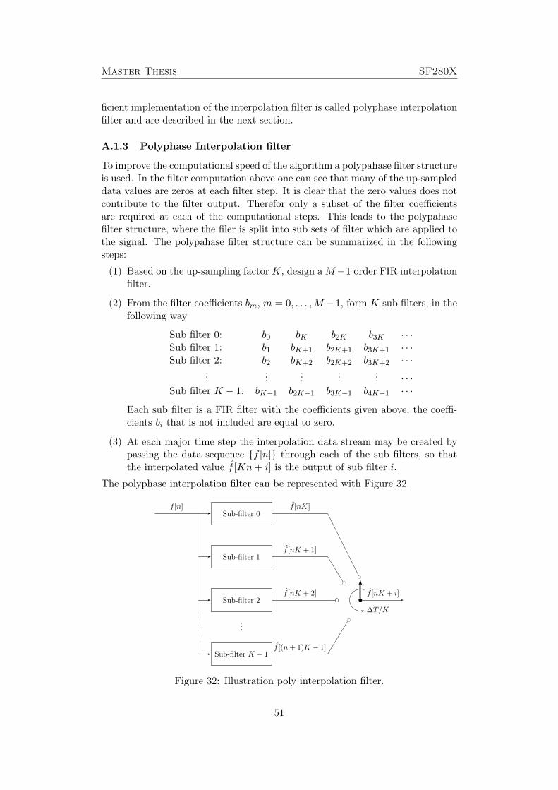
Master Thesis SF280X
ficient implementation of the interpolation filter is called polyphase interpolationfilter and are described in the next section.
A.1.3 Polyphase Interpolation filter
To improve the computational speed of the algorithm a polypahase filter structureis used. In the filter computation above one can see that many of the up-sampleddata values are zeros at each filter step. It is clear that the zero values does notcontribute to the filter output. Therefor only a subset of the filter coefficientsare required at each of the computational steps. This leads to the polypahasefilter structure, where the filer is split into sub sets of filter which are applied tothe signal. The polypahase filter structure can be summarized in the followingsteps:
(1) Based on the up-sampling factor K, design aM−1 order FIR interpolationfilter.
(2) From the filter coefficients bm, m = 0, . . . ,M −1, form K sub filters, in thefollowing way
Sub filter 0: b0 bK b2K b3K · · ·Sub filter 1: b1 bK+1 b2K+1 b3K+1 · · ·Sub filter 2: b2 bK+2 b2K+2 b3K+2 · · ·
......
......
... · · ·Sub filter K − 1: bK−1 b2K−1 b3K−1 b4K−1 · · ·
Each sub filter is a FIR filter with the coefficients given above, the coeffi-cients bi that is not included are equal to zero.
(3) At each major time step the interpolation data stream may be created bypassing the data sequence {f [n]} through each of the sub filters, so thatthe interpolated value f [Kn+ i] is the output of sub filter i.
The polyphase interpolation filter can be represented with Figure 32.
Sub-filter 0
Sub-filter 1
Sub-filter 2
Sub-filter K − 1
...
f [n] f [nK]
f [nK + 1]
f [nK + 2]
f [(n + 1)K − 1]
f [nK + i]
∆T/K
Figure 32: Illustration poly interpolation filter.
51

SF280X Master Thesis
When using the polyphase structure it is not necessary to preform the up-sampling step of inserting zeros in to the data sequence.
A.1.4 Down-sampling (or Decimation) by an Integer Factor
By down-sample a signal one want to increase the sampling interval ∆T by afactor L (or decreasing the samplings frequency with L). This is done by retainevery L sample of the original sequence {f [n]} by letting f [n] = f [Ln], where{f [n]} is the down-sampled sequence. However caution must be taken to preventaliasing effects in the down-sampled sequence. One can not directly down-samplea sequence unless it is known that the spectrum of the data sequence is equal tozero for all frequencies at and above the new Nyquist frequency defined by thenew sampling frequency. To prevent aliasing effects in the resampled data, are theoriginal sequence passed through a digital low-pass filter before down-sampled..
A.1.5 Resampled with non-integer factor
Assume that one want to resample a sequence to non-integer factor P and assumethat the factor P can be expressed as a rational factor
P =K
L, (A.6)
where K and L are integers. Then the resampling can be achieved by up-samplethe sequence by a factor K followed by a down-sample of the sequence by a factorL. Since the low pass filtering parts of the up- and down sapling are cascaded,see Figure 33a. The two filters may be replaced by a single filter, see Figure 33b.
Up-samplerInterpolation
filterAnti-aliasing
filterDown-sampler
f [n] f [n]
Interpolation Decimation
(a) Illustration of filters in the resample algorithm.
Up-samplerLow-pass
filterDown-sampler
f [n] f [n]
(b) Illustration of filters in compact form.
Figure 33: Illustration of filtering process for the resample algorithm.
For resampling factors P that are irrational one first has to approximate thefactor P with a rational number.
A.1.6 Kaiser window
A Kaiser window is given by the following equation
w[n] =
I0
(β
√1−
(n−N/2N/2
)2)
I0, n = 0; . . . , N − 1. (A.7)
52

Master Thesis SF280X
Where β is the Kaiser window parameter and I0 is the zeroth-order modifiedBessel function of the first kind, given by
I0(z) =∞∑k=0
(z2
4
)kk!Γ(k + 1)
. (A.8)
Where Γ is the Gamma function, Γ(n) = (n− 1)!.
53

SF280X Master Thesis
References
[1] Victor C Chen. The micro-Doppler effect in radar. Artech House, 2011.
[2] Johan Clemedson. Audio generation from radar signals, for target classifi-cation. Master’s thesis, KTH, 2017.
[3] Charles Cook. Radar signals: An introduction to theory and application.Elsevier, 2012.
[4] Per Enqvist. Spectral estimation by geometric, topological and optimizationmethods. PhD thesis, KTH, 2001.
[5] Ulf Carlsson Hans Bodén, Kjell Ahlin. Applied Signal Analysis. KTH Farkostoch Flyg / MWL, 2014.
[6] Chih-Wei Hsu, Chih-Chung Chang, Chih-Jen Lin, et al. A practical guideto support vector classification. 2003.
[7] Guy Kouemou, Christoph Neumann, and Felix Opitz. Sound and dynamicsof targets—fusion technologies in radar target classification. In InformationFusion, 2008 11th International Conference on, pages 1–7. IEEE, 2008.
[8] Justin Leo Cheang Loong, Khazaimatol S Subari, Muhammad Kamil Abdul-lah, Nurul Nadia Ahmad, et al. Comparison of mfcc and cepstral coefficientsas a feature set for pcg biometric systems. World Academy of Science, Engi-neering and Technology, International Journal of Medical, Health, Biomed-ical, Bioengineering and Pharmaceutical Engineering, 4(8):335–339, 2010.
[9] Bassem R Mahafza. Radar systems analysis and design using MATLAB.CRC press, 2002.
[10] Thin Thin Mar, Su Su Yi Mon, et al. Pulse compression method for radarsignal processing. International Journal of Science and Engineering Appli-cations, 3:31–35, 2014.
[11] Andrew Ng. Cs229 lecture notes, part v, support vector machines.
[12] Rajkumar Palaniappan and Kenneth Sundaraj. Respiratory sound classi-fication using cepstral features and support vector machine. In IntelligentComputational Systems (RAICS), 2013 IEEE Recent Advances in, pages132–136. IEEE, 2013.
[13] Lawrence R Rabiner. Multirate digital signal processing. Prentice Hall PTR,1996.
[14] Graeme E Smith, Karl Woodbridge, and Chris J Baker. Template basedmicro-doppler signature classification. In High Resolution Imaging and Tar-get Classification, 2006. The Institution of Engineering and Technology Sem-inar on, pages 127–144. IET, 2006.
54
Master Thesis SF280X
[15] Rao Sreenivasa and Shashidhar G Koolagudi. Robust emotion recognitionusing spectral and prosodic features. Springer Science & Business Media,2013.
[16] Jerome Friedman Trevor Hastie, Robert Tibshirani. The elements of statis-tical learning: data mining, inference and prediction. Springer, 2009.
[17] Christian Wolff. Radar Basics derivation of the doppler-frequency formula.
[18] Christian Wolff. Radar basics: Classification of radar sets, radar frequencybands. Radartutorial. eu, 2014.
[19] Christian Wolff. Radar basics: Radar antennas. Radartutorial. eu, 2014.
[20] Christian Wolff. Radar basics: Radar basic principles. Radartutorial. eu,2014.
[21] Christian Wolff. Radar basics: Radar transmitter. Radartutorial. eu, 2014.
[22] Dong Yu and Li Deng. Automatic speech recognition: A deep learning ap-proach. Springer, 2014.
[23] Hwanjo Yu and Sungchul Kim. Svm tutorial—classification, regression andranking.
[24] Qun Zhang, Ying Luo, and Yong-an Chen. Micro-Doppler Characteristicsof Radar Targets. Elsevier, 2016.
55


TRITA -MAT-E 2017:63
ISRN -KTH/MAT/E--17/63--SE
www.kth.se