radar-based nowcasting and verification techniques
TRANSCRIPT

Radar-Based Nowcasting and Verification Techniques
Erik Becker
Research Scientist
Typhoon Committee Roving Seminar 13 November 2019

Lecture Topics
Topic B – Rain gauge and radar data processing for QPE/QPF
Goal: Scrutinise the radar processing chain for accurate QPE and QPF
1. Radar and Rain-Gauge Data Quality and Processing2. Radar Precipitation and Rain-Gauge Adjustment Techniques3. Radar-Based Nowcasting and Verification Techniques
Reading Material:• Wang, Yong, Estelle De Coning, Wilfried Jacobs, Paul Joe, Larisa Nikitina, Rita Roberts,
Jianjie Wang, et al. 2017. “Guidelines for Nowcasting Techniques.” WMO.https://library.wmo. int/opac/doc_num.php?explnum_id=3795
• Pierce, Clive, Alan Seed, Sue Ballard, David Simonin, and Zhihong Li. 2012. “Nowcasting.” In Doppler Radar Observations - Weather Radar, Wind Profiler, IonospericRadar, and other Advanced Applications, by Joan Bech and Jorge Luis Chau, 97-142.
Examples from SAWS and MSS Radar networks.

Outline
Radar Precipitation
• Intro and outline
• Nowcasting
– Object based tracking
– Field Advection
– Growth and Decay (stochastic and ANN model)
– NWP
– Blending
• Verification
– CT performance diagram
– Spatial (FSS, SAL, etc)
• Some Operational considerations
• Summary
Useful Tools
PYTHON:
• LROSE: https://github.com/NCAR/lrose-core
• pySTEPS: https://github.com/pySTEPS
• SwirlsPy: https://docs.com-swirls.org/
R:
• SpatialVx package (Spatial Verification Tools)
• Verification package (Standard Verification Tools)

Nowcasting

Object-Based (Cell) Tracking
Thunderstorm Identification Tracking And Nowcasting:
• TITAN (NCAR). https://github.com/NCAR/lrose-titan
• Identifies thunderstorm through single threshold
– Typically 30dBZ
• Dual Threshold also possible (Useful for squall lines)
• Storm Properties can be calculated:
– Volumetric centroid
– Volume (km3)
– Mean area (km2)
– Precipitation flux (m3/s)
– Mass (ktons)
– Max, Mean dBZ
– Etc… (Many more)

Bloemfontein - 24 Feb 2015
Object-Based (Cell) Tracking
Threshold only 30dBZ Threshold (30dBZ) + convective classification• Convective Classification
• Texture algorithm:
• Improves hail metrics and warnings
𝑡𝑒𝑥𝑡𝑢𝑟𝑒 = 𝑠𝑑𝑒𝑣 𝑑𝑏𝑧2

Object-Based (Cell) Tracking
• Need at least 2 time steps• Matching using overlaps and optimization.• Handles storm merging and splitting.
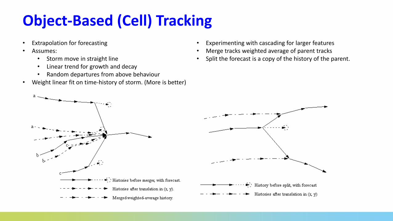
Object-Based (Cell) Tracking• Extrapolation for forecasting• Assumes:
• Storm move in straight line• Linear trend for growth and decay• Random departures from above behaviour
• Weight linear fit on time-history of storm. (More is better)
• Experimenting with cascading for larger features• Merge tracks weighted average of parent tracks• Split the forecast is a copy of the history of the parent.
Object-Based (Cell) Tracking
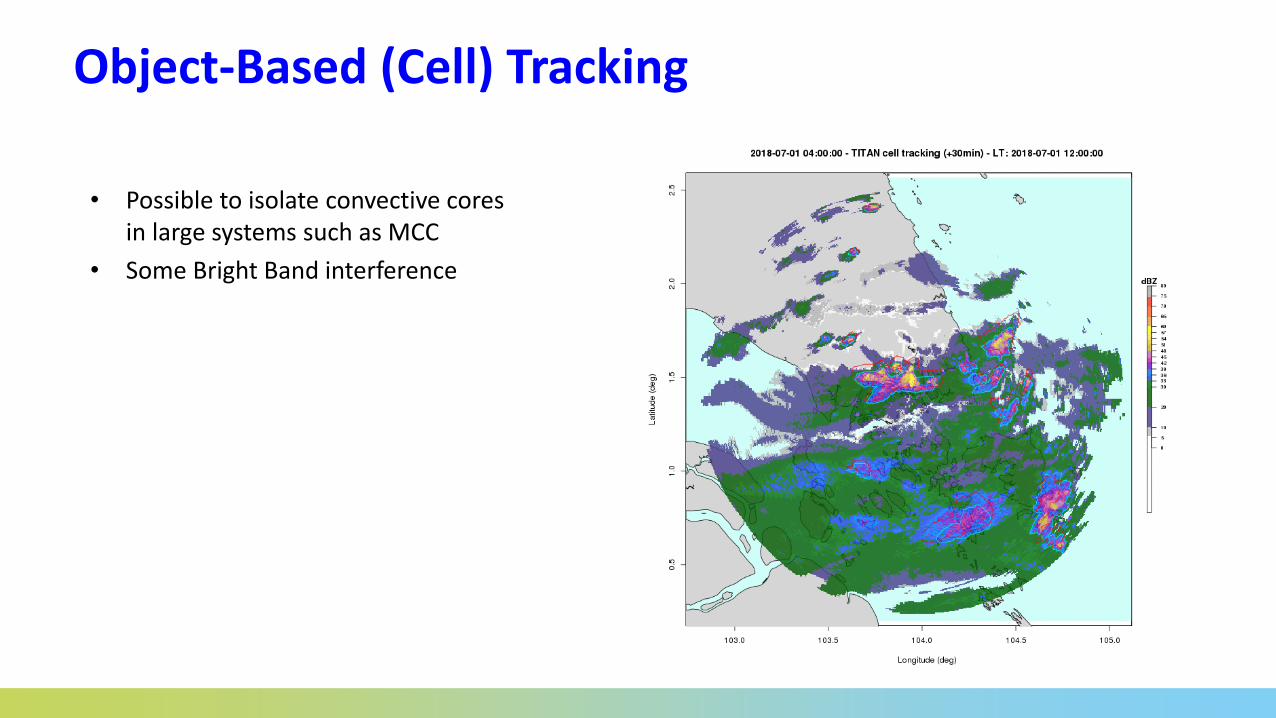
• Possible to isolate convective cores in large systems such as MCC
• Some Bright Band interference

Field Advection (Extrapolation):
• Motion vectors calculated from current and previous radar images.
• Results can be noisy due to temporal variability of reflectivity.
• Using additional time steps can help smooth vectors.
• Linear or Rotational flow.
• Methods (pySTEPS, SwirlsPy):
– COTREC (SWIRLS)
– Vibrational Echo Tracking (VET) (MAPLE)
– Optical Flow:
• Open CV (Lukas-Darts
• Rover
• Semi-Lagrangian backward interpolation scheme to extrapolate reflectivity.
• Does not consider growth and decay.
• Sensitivity to settings, weather type and domain.
• Consider computation efficiency.
• RainyMotion, constant motion vector for domain (Benchmark)
𝐷𝑡𝑍 = 𝑢𝛿𝑍
𝛿𝑥+ 𝑣
𝛿𝑍
𝛿𝑦+𝛿𝑍
𝛿𝑡= 0
Solve using Minimize Least Squares

Motion vector calculationsUWND VWND
• Sensitivity study on optical flow parameters:
– Box window size
– Interpolation methods
– Max speed
– Etc.
• Different weather types may require different settings
Nearest Neighbour
Inverse Distance Weighting

Nowcasting Methods: Optical Flow Extrapolation
Observed Forecast
• 3 hour extrapolation• Advection appears to be slower than the observed

Challenge in the Tropics
Extrapolation at 0430 UTC (T-30min – T+120min)
TITAN cell tracking at 0400 UTC – 0500 UTC
(30min forecast track)

Growth and Decay
• Rainfall has a scaling structure in both space and time
• Multiplicative cascades can model this behaviour
• The Weather and Climate, Lovejoy and Schertzer, 2013, Cambridge University Press
• Statistical Approach (Stochastic Noise)Lovejoy et al., 1987
J. Geophys. Res.
Information courtesy Alan Seed

pySTEPS - Decomposition
• Cascade Decomposition
• Optical Flow vectors for each cascade level.
• Semi-Lagrangian Extrapolation.
• Growth and decay:
– Large Scale features to persist.
– Stochastic noise.
• Fourier Domain
• Auto-Regressive Model
Stochastic Noise Generation:
Multiplicative Cascades:

pySTEPS
• 3 hour forecast
• Stochastic noise makes is possible to produce ensemble
• Probabilistic forecast now possible
• Will require a study on how to approach different weather systems
Observed Ensemble 1
Ensemble 2 Ensemble 3

Deep learning algorithm Radar data for the previous 50 minutes (10 frames)
Output:Predicted radar maps for 0-3 hours, depending on the weather systems
Input: observed radar maps up to current time
Why DLM ? • Learn the nonlinear characteristics in real time• Provide the possibility of predicting thunderstorms before they appear from radar
Artificial Neural Network (ANN) Nowcaster

Artificial Neural Network (ANN)
• Current setup not ideal.• ANN will require a different processing
approach and thus needs to be redeveloped.
• ANN requires excessive amounts of data.• Needs this info to model storm initiation,
evolution and movement.
Good Case
Bad Case
Contribution: WSD

Numerical Weather Prediction (NWP)
Considerations:
• Domain Size
• Initial condition for regional model
• High resolution
– Convective resolving
– Urban area (land use)
• Data Assimilation
– 3D-VAR or 4D-VAR
• Cycling (Cold vs Warm start, Spin-up)
• Forecast length (typical 48 hour for regional domain)
• For nowcasting, important to get your precipitation, humidity, winds and temperature observation right.
• Accurate initial conditions one of the biggest problems
Regional version of Met-Office Unified Model - SINGV 1.5km

Global ECMWFO (10 km)
NWP SINGVO (1 km)
Urban uSINGVO (100 m)
• Urban Model nested domain is 180 km x 180 km in horizontal and extends up to 40 km up in the atmosphere, centred over Singapore.
• Initial and boundary conditions come from ECMWF NWP model.
Urban morphology and land-use• Morphological parameters W/R, H/W, H
are calculated from 2D topographic dataprovided by Singapore Land Authority(LOD2).
• ESA CCI land-use data (~ 300 m) with somemodifications making it more appropriatefor Singapore.
Future Work:
• Model geared more towards a nowcasting setup:
• Hourly cycle (Warm start)
• Data Assimilation (3D-VAR):
– Himawari-8 radiances [AMV’s]
– Radar derived rain-rates [Radial Velocities]
• Forecast range up to 6 hours
• High Resolution (300m) - Nested
NWP – High Resolution Urban Model for Singapore
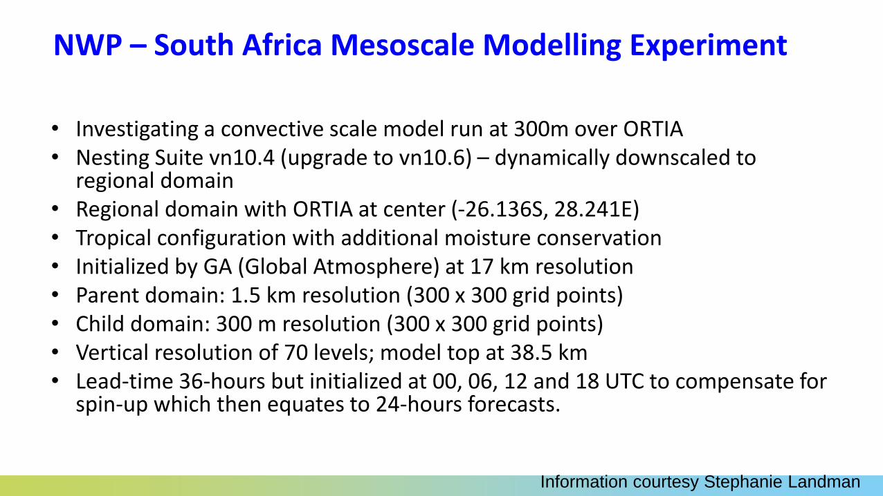
NWP – South Africa Mesoscale Modelling Experiment
• Investigating a convective scale model run at 300m over ORTIA• Nesting Suite vn10.4 (upgrade to vn10.6) – dynamically downscaled to
regional domain• Regional domain with ORTIA at center (-26.136S, 28.241E)• Tropical configuration with additional moisture conservation • Initialized by GA (Global Atmosphere) at 17 km resolution• Parent domain: 1.5 km resolution (300 x 300 grid points)• Child domain: 300 m resolution (300 x 300 grid points)• Vertical resolution of 70 levels; model top at 38.5 km • Lead-time 36-hours but initialized at 00, 06, 12 and 18 UTC to compensate for
spin-up which then equates to 24-hours forecasts.
Information courtesy Stephanie Landman

High Resolution Mesoscale Modellin• Convective scale model (300 m) using the UK Met Office Unified Model
• Investigating a convective scale model run at 300m over ORTIA
• Model simulations for 2016-11-02 • Storm moved over OR Tambo Int.
Airport – Flooding of airport access roads and parking structures
• Severe impact on airport operations
• Red (1,5 km) & Purple (300 m)• 300x300 (shaded) & 600x600 (non-
shaded)• Black circle ORTIA aerodrome
Information courtesy Stephanie Landman

Unified Model (300m)
Information courtesy Stephanie Landman

Unified Model (300m)
Information courtesy Stephanie Landman

Radar and NWP BlendingBoM – STEPS system
Radar NWP Noise Blend
+ w0n X
+ w2n X
+ w3n X
+ w4n X
+ w5n X
+ w1n X
+ w0f X
+ w1f X
+ w3f X
+ w4f X
+ w5f X
+ w2f X
w0r X
w1r X
w2r X
w3r X
w4r X
w5r X
=
=
=
=
=
=
Forecast
• Need to merge Radar with NWP to include dynamical evolution of the atmosphere
• NWP downscaled to be statistically equivalent to rain analysis
• Weight are calculated from the expected skill (variance) of the advection and NWP forecasts

Obs Radar
BlendingNWP
Blend
Advection
Flooding event at forecast time.
Radar Time: 2018-10-10 08h45 UTCNWP initialisation time: 2018-10-09 12Z
SINGV-DS 1.5km
Forecast Time: 2018-10-10 10h00 UTC

Radar Nowcasting: Future Work
• Goal: Blending
• Sensitivity study with nowcasting parameters
• Improve on verification technique.– Compensate for domain
– Classification of dBZ
Radar Extrapolation:
Advection
Growth and Decay:
pySTEPSANN
NWP:Nowcasting
Setup
Lead-Time: 0 – 6 hours

Verification

Why Verify?
To answer questions on:
• Model performance with forecasting the weather (location, type, etc.)
• Administrative (choice of model / continuous monitoring)
• Scientific understanding (improve model dynamics/parametrization)
• Economic (Disaster management / Decision support)
References:• CAWCR verification website (Beth Ebert): http://www.cawcr.gov.au/projects/verification/
• Jolliffe IT and Stephenson DB (2011) Forecast Verification: A Practictioner’s Guide in Atmospheric Science (2nd Ed). Wiley.
• Wilks DS (2011) Statistical Methods in the Atmospheric Sciences (3rd Ed). Academic Press.
• Casati, B., Wilson, L. J., Stephenson, D. B., Nurmi, P., Ghelli, A., Pocernich, M., Damrath, U., Ebert, E. E., Brown, B. G. and Mason, S. (2008), Forecast verification: current status and future directions. Met. Apps, 15: 3–18.
• WMO research programme: https://www.wmo.int/pages/prog/arep/wwrp/new/Forecast_Verification.html

What makes a good forecast?
• A forecast must have Consistency, be of good Quality and be of Value• Need to determine or VERIFY that a forecast has these qualities.
• Forecast Attributes:– Bias (deviate from the mean observations) – Association (linear relationship or correlation), – Accuracy (difference from the observed error), – Skill (compared to some reference, climatology or persistence), – Reliability (agreement between observed and forecast values), – Resolution (resolve events into subset of events), – Sharpness (extreme values), – Discrimination (higher prediction frequency for specific outcomes), – Uncertainty (variability)
• Ground Truth – Normally from observations or reanalysis. Consider the limitations of the observation.

Verification Methods
Standard:
• Dichotomous (yes/no) forests
• Multi-category forecasts
• Continuous variable
• Probabilistic forecasts (Brier Skill Score)
Diagnostic (scientific):
• Spatial Forecasts
• Probabilistic forecasts, including ensemble prediction systems (Rank Histogram)
• Rare events (EDS, SEDI, SEDS)

Verification - Histograms
• Univariate Statistics; Good place to start.
• Frequency histograms
• Separate into different thresholds
• Good way to gee how model performs at different intensities
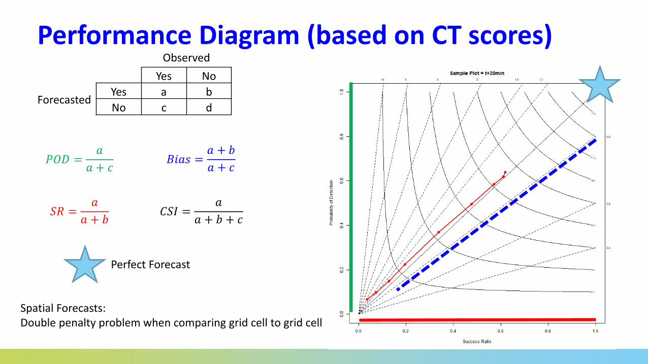
Performance Diagram (based on CT scores)Observed
Yes No
ForecastedYes a b
No c d
𝑃𝑂𝐷 =𝑎
𝑎 + 𝑐
𝑆𝑅 =𝑎
𝑎 + 𝑏
𝐵𝑖𝑎𝑠 =𝑎 + 𝑏
𝑎 + 𝑐
𝐶𝑆𝐼 =𝑎
𝑎 + 𝑏 + 𝑐
Perfect Forecast
Spatial Forecasts: Double penalty problem when comparing grid cell to grid cell
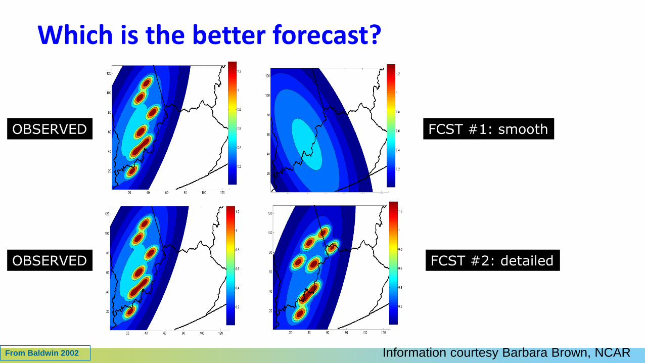
Which is the better forecast?
OBSERVED
FCST #1: smooth
FCST #2: detailed
OBSERVED
From Baldwin 2002 Information courtesy Barbara Brown, NCAR

CT Score for grid comparison
Verification Measure Forecast #1
(smooth)
Forecast #2
(detailed)
Mean absolute error 0.157 0.159
RMS error 0.254 0.309
Bias 0.98 0.98
CSI (>0.45) 0.214 0.161
GSS (>0.45) 0.170 0.102
From Baldwin 2002 Information courtesy Barbara Brown, NCAR

Neighbourhood Techniques
• Define Domains of interest (Scale dependent)Observed
Yes No
ForecastedYes a b
No c d
𝑃𝑂𝐷 =𝑎
𝑎 + 𝑐
𝑆𝑅 =𝑎
𝑎 + 𝑏
𝐵𝑖𝑎𝑠 =𝑎 + 𝑏
𝑎 + 𝑐
𝐶𝑆𝐼 =𝑎
𝑎 + 𝑏 + 𝑐

Spatial Verification Approaches
• To address limitations of traditional approaches
• Goal is to provide more useful information about forecast performance
Information courtesy Barbara Brown, NCAR

← length scale 3 →
1 1
1 1
𝑀𝑆𝐸 =1
𝑁
𝑖=0
𝑁
𝐹𝑖 − 𝑂𝑖2
𝑀𝑆𝐸𝑟 =1
𝑁
𝑖=1
𝑁
𝐹𝑖2 + 𝑂𝑖
2
𝑭𝒓𝒂𝒄𝒕𝒊𝒐𝒏𝒔 𝑺𝒌𝒊𝒍𝒍 𝑺𝒄𝒐𝒓𝒆(𝒏) = 𝟏 −𝑴𝑺𝑬(𝒏)
𝑴𝑺𝑬(𝒏)𝒓
𝑀𝑆𝐸 =1
𝑁
𝑖=0
𝑁
𝐹𝑖 − 𝑂𝑖2
Forecast
1
1
1
Roberts, N. M. and Lean, H. W. (2008)
← length scale 5 →
1/9
3/25
Observation
← length scale 3 →
0
2/25
← length scale 5 →
Fractions Skill Score (FSS)
n = Length scale
Length scale are selected so that n x n grid box doubles in size with each iteration (i.e. 2 km → 270 km)
Back

TITAN FSS• FFS Scores for TITAN cell tracking• 3 day period 2018-11-09 to 2018-11-11• TITAN (blue) compared to Persistence (red)• 10th, 50th and 90th percentile plot for the evaluation period• Length scales 4km, 16km and 64km

FSS Scores Nowcasting systems
15 dBZ
35 dBZ

Info from M .Mittermaier: 4th Int'l Verification Methods Workshop, Helsinki, 4-6 June 2009
1. Is the domain average precipitation correctly forecast? A = 0.21
2. Is the mean location of the precipitation distribution in the domain correctly forecast? L = 0.06
3. Does the forecast capture the typical structure of the precipitation field (e.g., large broad objects vs. small peaked objects)? S = 0.46
(perfect=0)
observed forecast
Structure-Amplitude-Location (SAL)Wernli et al., Mon. Wea. Rev., 2008

Mode – SpatialVx
Information courtesy Stephanie Landman

Operational Requirements

Operational: Considerations
Display
Modelling
Quality Control
Observation• Data point for incoming data (Availability, Latency).
• Data Format (HDF5, RB5, IRIS, NETCDF, MDV, etc.)
• Distinguish between online/offline data.
• Distinguish between research/operational.
• Processing of data to radar, nowcasting, verification, etc. type products (Server, HPC).
• Archiving and Database management.
• Visualisation (Webpage, Software).
• House Keeping.
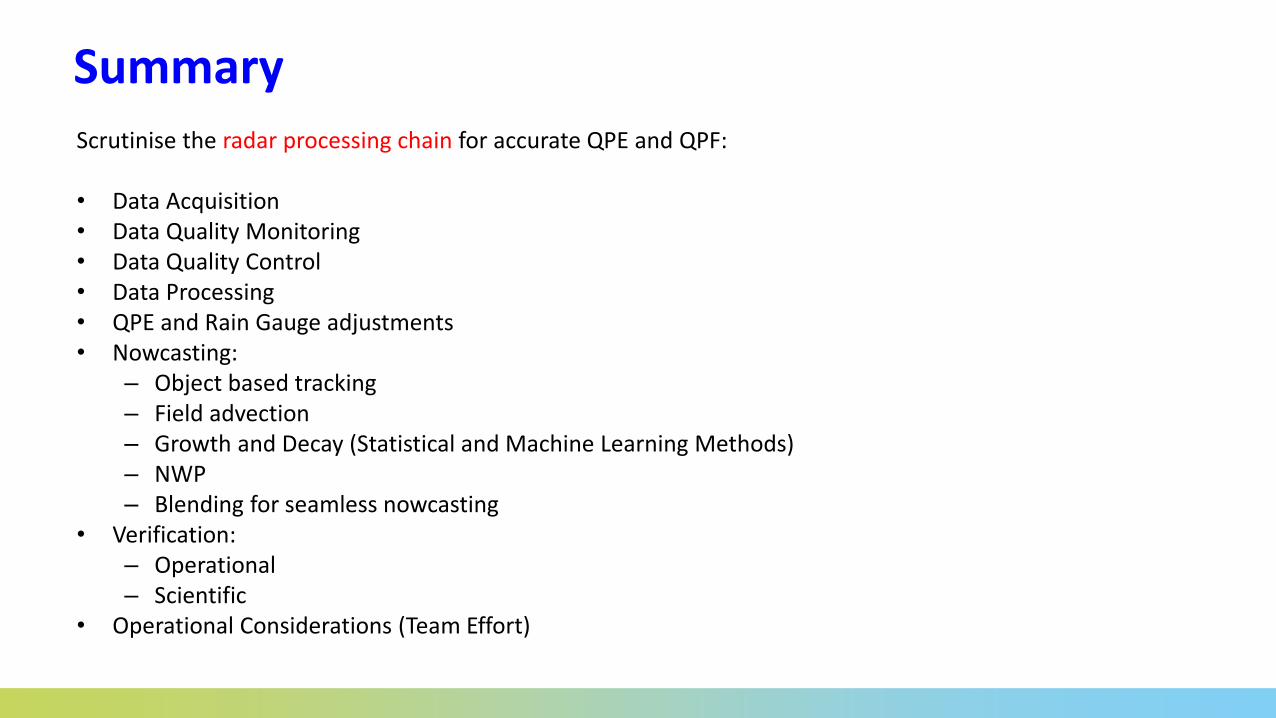
SummaryScrutinise the radar processing chain for accurate QPE and QPF:
• Data Acquisition • Data Quality Monitoring• Data Quality Control • Data Processing• QPE and Rain Gauge adjustments• Nowcasting:
– Object based tracking– Field advection– Growth and Decay (Statistical and Machine Learning Methods)– NWP– Blending for seamless nowcasting
• Verification:– Operational– Scientific
• Operational Considerations (Team Effort)
