racial disparities in mortality risks in a sample of the …

Johns Hopkins University, Dept. of Biostatistics Working Papers

5-7-2007

RACIAL DISPARITIES IN MORTALITY RISKSIN A SAMPLE OF THE U.S. MEDICAREPOPULATIONYijie ZhouDepartment of Biostatistics, Johns Hopkins Bloomberg School of Public Health, [email protected]

Francesca DominiciDepartment of Biostatistics, The Johns Hopkins Bloomberg School of Public Health

Thomas A. LouisDepartment of Biostatistics, Johns Hopkins University Bloomberg School of Public Health

This working paper is hosted by The Berkeley Electronic Press (bepress) and may not be commercially reproduced without the permission of thecopyright holder.Copyright © 2011 by the authors

Suggested CitationZhou, Yijie ; Dominici, Francesca; and Louis, Thomas A., "RACIAL DISPARITIES IN MORTALITY RISKS IN A SAMPLE OFTHE U.S. MEDICARE POPULATION" (May 2007). Johns Hopkins University, Dept. of Biostatistics Working Papers. Working Paper145.http://biostats.bepress.com/jhubiostat/paper145

http://biostats.bepress.com/jhubiostat

Racial Disparities in Mortality Risks

in a Sample of the U.S. Medicare Population

Yijie Zhou, Francesca Dominici and Thomas A. Louis ∗

May 7, 2007

Abstract

Racial disparities in mortality risks adjusted by socioeconomic status (SES) are not well under-

stood. To add to the understanding of racial disparities, we construct and analyze a data set that

links, at individual and zip code levels, three government databases: Medicare, Medicare Current

Beneficiary Survey and U.S. Census. Our study population includes more than 4 million Medicare

enrollees residing in 2095 zip codes in the Northeast region of U.S. We develop hierarchical models

to estimate Black-White disparity in risk of death, adjusted by both individual-level and zip code-

level income. We define population-level attributable risk (AR), relative attributable risk (RAR) and

odds ratio (OR) of death comparing Blacks versus Whites, and we estimate these parameters using

a Bayesian approach via Markov chain Monte Carlo. By applying the multiple imputation method

to fill in missing data, our estimates account for the uncertainty from the missing individual-level

income data. Results show that for the Medicare population being studied, there is a statistically and

substantively significantly higher risk of death for Blacks compared with Whites, in all three measures

∗Yijie Zhou is Graduate Student (email: [email protected]); Francesca Dominici is Professor (email: [email protected]); and Thomas A. Louis is Professor, Department of Biostatistics, Johns Hopkins University, Baltimore,MD, 21205 (email: [email protected]). Support for this work was provided by the National Institute for EnvironmentalHealth Sciences (ES012054-03) and by the Environmental Protection Agency (RD83054801).

1

Hosted by The Berkeley Electronic Press

of AR, RAR, and OR, both adjusted and not adjusted for income. In addition, after adjusting for

income we find statistically significant reduction of AR but not of RAR and OR.

Keywords: Hierarchical Model; Markov chain Monte Carlo; Multiple Imputation; Racial Disparity; So-

cioeconomic Status.

1 INTRODUCTION

There is considerable evidence and concern about health disparities between the majority white pop-

ulation and minority racial groups in the Unite States, especially the disparities between Blacks and

Whites. Social epidemiology literature suggests that the Black-White disparities in health and mortality

are due to the differentiation of social and historical factors which can be summarized into the following

three categories (Hummer (1996); Williams (1999)): (1) differentiation in socioeconomic status (SES);

(2) racism: both institutional (residential segregation, racial isolation and political representation) and

individual (majority-group behavior and attitude, perception of discrimination); (3) culture and behavior

differences. In order to understand how race is associated with health and mortality, it is important

to investigate the relative importance of different factors, with SES being the most studied in the past

several years.

SES differentiation explains racial disparities in mortality risks at both individual and area levels (LeClere

et al. (1997)). It is well known that individual-level SES is associated with race and is a strong predictor

of mortality risks (Williams and Collins (1995); Link and Phelan (1995)). On the other hand, area-

level SES is associated with both mortality risks and individual-level SES (Pickett and Pearl (2001)).

Therefore, failure to account for area-level SES would result in biased estimation of the association

between race, individual-level SES, and mortality risks (Cole and Hernan (2002); Robins and Greenland

(1992)).

For the relation between area-level SES and health, literature suggests that besides the association

between health and absolute SES level of the area (e.g. median income), the SES inequality within the

2

http://biostats.bepress.com/jhubiostat/paper145

area, i.e., the difference between the SES of the well off and the poor off, is also associated with health

and mortality (Kawachi and Kennedy (1999)). In analyses performed at small geographic areas such as

census tracks or zip codes, the absolute SES level tends to be more strongly associated with mortality

rates than the SES inequality, while the situation is reversed in analyses at larger areas such as states or

countries. Some commonly used inequality measures for income are inter-quartile range, Robin Hood

Index, Gini Coefficient (Wilkinson (1997); Lochner et al. (2001); McLaughlin and Stokes (2002)).

Several studies have analyzed the individual-level relation between race, SES and mortality risks (Cooper

et al. (2001); Howard et al. (2000); Guralnik et al. (1993); Keil et al. (1992); LeClere et al. (1997); Otten

et al. (1990); Smith et al. (1998); Sorlie et al. (1995, 1992); Steenland et al. (2004)). However, most

of these studies are either restricted to a specific and small geographic area (Guralnik et al. (1993); Keil

et al. (1992)), or targeted on premature mortality for people younger than 65 years old (Cooper et al.

(2001); Otten et al. (1990); Smith et al. (1998); Steenland et al. (2004)). In addition, these studies

generally do not account for the potential confounding of area-level SES, and do not use hierarchical

models for the analysis. Such models are necessary to account for the intra-area correlation between

individuals, as well as the between-area spatial correlation. Another study by Gornick et al. (1996)

analyzes the relationship between race, SES and mortality rates for the nation-wide elderly population

over 65 years old. However, the analysis is performed at zip code level instead of individual level.

In this paper we develop and apply hierarchical models to investigate the following questions:

1. What is the association between an individual’s race and risk of death adjusted by age and gender?

2. How will this association vary when we adjust for both individual- and area-level SES?

To address these questions, we integrate three large government databases with information on individual

race, age, gender, date of death, individual-level SES and zip code-level SES over the period 1999-2002,

for more than 4 million people residing in 2095 zip codes in the Northeast region of the United States.

Using this data set, we develop and apply hierarchical statistical models to explore the association

between individual race and mortality risks, as well as whether this association is explained by the racial

3


differentiation in both individual-level and zip code-level income. Based on these models, we carry out

sensitivity analysis to identify which summary of individual-level income at zip code level (e.g., mean or

inter-quartile range (IQR)) explains most the variability in mortality risks. We measure the association

between race and mortality risks using population-level attributable risk (AR), relative attributable

risk (RAR) and odds ratio (OR) of death comparing Blacks versus Whites. These parameters are

defined as functions of model predicted probabilities which can be easily estimates by use of a Bayesian

approach via Markov chain Monte Carlo (MCMC).

In Section 2, we describe the data sources. In Section 3 we describe the methods for the analysis,

including hierarchical models, definition of association measures, and multiple imputation for missing

data. Section 4 presents the results. Section 5 is the sensitivity analysis and discussion in Section 6 is

followed. The statistical and computational details are in the Appendix.

2 DATA SOURCES

To explore the association between race and mortality risks adjusted by SES, we construct a data set

that links, at individual and zip code levels, three government databases: Medicare, U.S. Census and

Medicare Current Beneficiary Survey (MCBS). The Medicare data set includes individual race, age,

gender and date of death over the period 1999-2002 for more than 4 million black and white Medicare

enrollees who are 65 years and older residing in 2095 zip codes in the Northeast region of U.S. People

who are younger than 65 at enrollment are eliminated because they are eligible for the Medicare program

due to the presence of either a certain disability or End Stage Renal Disease (ESRD) and therefore do

not represent the general Medicare population.

Figure 1 shows the study area which includes 2095 zip codes in 64 counties in the Northeast region of

U.S. We choose the counties based on whether the locations of their geographical centers fall within a

desired range which covers the Northeast coast region of U.S. We exclude zip codes without available

study population or Census information. This area covers most of the large, urban cities including

4


Washington D.C., Baltimore MD, Philadelphia PA, New York City NY, New Haven CT, Providence RI

and Boston MA. It has the advantage of high population density, racial diversity and substantial SES

heterogeneity.

We categorize the age of individuals into 5 intervals based on age at enrollment: [65, 70), [70, 75),

[75,80), [80, 85), and [85, +). This categorization facilitates the detection of age effects on mortality

risks, because the difference in mortality risks for one year increase in age is relatively small. We

“coarsen” the daily survival information into yearly survival indicators. As is the case for most survival

analyses, the annual survival records for each individual are modelled as conditionally independent, in

our case as inputs to logistic regression. Therefore, we define our outcome “individual’s risk of death”

as the probability of the occurrence of death for an individual in one year. This prevents comparing

individuals with different risks of observing their events of death due to the difference in the length of

follow-up.

We link the Medicare data set to the 2000 U.S. Census database by zip code. We obtain zip code-level

SES using median household income from the Census data.

Individual-level SES data are available only for the subset of the Medicare population who participate

the Medicare Current Beneficiary Survey (MCBS). Figure 1 shows the zip codes with MCBS enrollment

in the study area. The MCBS data set consists of records for approximately 1,700 Medicare enrollees

within 410 zip codes in the study area, approximately 0.04% of the study population. We collect

individual-level SES from the MCBS data set using yearly income of the surveyed person and his/her

spouse if there is any.

5


3 METHODS

3.1 Hierarchical Models

Guided by the scientific questions in section 1, we define two hierarchical models for estimating the

individual-level association between race and risk of death adjusted and not adjusted by individual- and

zip code-level income.

Let i denote individual, j denote zip code of residence, t denote year, and Dijt be the death indicator

for individual i in zip code j in year t. We define the model adjusted for income as

logit Pr(Dijt = 1) = α0 + α1 raceij + α2Xij + α01 incomej + U0j + U1j raceij + U2jXij , (1)

where Xij are individual-level covariates, specifically, ageij , genderij , ageij × genderij and incomeij ;

incomej is the zip code-level median household income. As stated in Section 2, we construct age

category, denoted by ageij , using age at enrollment and therefore, it does not vary with t. The

parameters α0, α1, α2 and α01 are fixed effects, whereas U0j , U1j ,U2j are zip code-level, correlated

random effects. We define the model not adjusted for income the same as (1) but leaving out covariates

incomeij and incomej .

3.2 Modelling Spatial Correlation

To account for unmeasured confounders that might vary spatially as the mortality risks, we allow

the random effects to be spatially correlated. Specifically, let Uj denote the random effects vector

(U0j , U1j ,U′2j)

′ for zip code j and let U denote the vector (U′1,U

′2, · · · ,U′

J)′ of the random effects of

all J zip codes, we assume the following distribution for the random effects:

U ∼ MV N(0,Σ). (2)

6


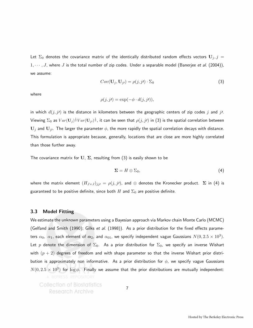
Let Σ0 denotes the covariance matrix of the identically distributed random effects vectors Uj , j =

1, · · · , J , where J is the total number of zip codes. Under a separable model (Banerjee et al. (2004)),

we assume:

Cov(Uj ,Uj′) = ρ(j, j′) · Σ0 (3)

whereρ(j, j′) = exp(−φ · d(j, j′)),

in which d(j, j′) is the distance in kilometers between the geographic centers of zip codes j and j′.

Viewing Σ0 as V ar(Uj)12 V ar(Uj′)

12 , it can be seen that ρ(j, j′) in (3) is the spatial correlation between

Uj and Uj′. The larger the parameter φ, the more rapidly the spatial correlation decays with distance.

This formulation is appropriate because, generally, locations that are close are more highly correlated

than those further away.

The covariance matrix for U, Σ, resulting from (3) is easily shown to be

Σ = H ⊗ Σ0, (4)

where the matrix element (HJ×J)jj′ = ρ(j, j′), and ⊗ denotes the Kronecker product. Σ in (4) is

guaranteed to be positive definite, since both H and Σ0 are positive definite.

3.3 Model Fitting

We estimate the unknown parameters using a Bayesian approach via Markov chain Monte Carlo (MCMC)

(Gelfand and Smith (1990); Gilks et al. (1998)). As a prior distribution for the fixed effects parame-

ters α0, α1, each element of α2, and α01, we specify independent vague Gaussians N(0, 2.5 × 103).

Let p denote the dimension of Σ0. As a prior distribution for Σ0, we specify an inverse Wishart

with (p + 2) degrees of freedom and with shape parameter so that the inverse Wishart prior distri-

bution is approximately non informative. As a prior distribution for φ, we specify vague Gaussians

N(0, 2.5 × 103) for log φ. Finally we assume that the prior distributions are mutually independent:

7


p(α0, α1,α2, α01,Σ0, φ) = p(α0)p(α1)p(α2)p(α01)p(Σ0)p(φ). We generate posterior samples of all un-

known parameters by implementing a Gibbs Sampler with Metropolis-Hastings (Geyer (1992); Smith

and Roberts (1993)) under R version 2.4.1. All inferences about the parameters are derived from these

posterior draws. Detailed formulas of the conditional distributions used in the Gibbs Sampler are in the

Appendix A. Burn-in consists of 2×104 iterations, and 5×103 iterations are used for posterior summaries.

Convergence of Markov chains is assessed using the Gelman and Rubin convergence statistic (Gelman

and Rubin (1992); Brooks and Gelman (1998)).

3.4 Association Measures

The common approach of reporting the association between race and mortality risks is to report the fixed

effect race coefficient α1 in (1), whose interpretation is subjected to the coding of the race covariate as

well as the conditional structure of the zip code-level random effects. Therefore, for direct understanding

of the difference in risk of death between the black and white populations, we report population-level

attributable risk (AR), relative attributable risk (RAR) and odds ratio (OR) of death comparing Blacks

versus Whites. This approach of reporting measures of associations that are functions of predicted values

has the advantage that their interpretation does not depend on model structure and parameterization

(e.g., on the conditional structure of random effects, and on covariate centering and scaling).

Let

Pijtb = Pr(Dijt = 1| raceij = Black,Xij = xij , Incomej = incomej ,θ)

Pijtw = Pr(Dijt = 1| raceij = White,Xij = xij , Incomej = incomej ,θ)

denote the predicted probabilities of death in year t for a black person and a white person, respectively,

whose other covariates values are the same as as the ith individual in the jth zip code, where θ denotes

8


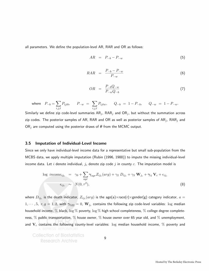
all parameters. We define the population-level AR, RAR and OR as follows:

AR = P···b − P···w (5)

RAR =P···b − P···w

P···w(6)

OR =P···bQ···wP···wQ···b

(7)

where P···b =∑i,j,t

Pijtb, P···w =∑i,j,t

Pijtw, Q···b = 1− P···b, Q···w = 1− P···w.

Similarly we define zip code-level summaries ARj , RARj and ORj , but without the summation across

zip codes. The posterior samples of AR, RAR and OR as well as posterior samples of ARj , RARj and

ORj are computed using the posterior draws of θ from the MCMC output.

3.5 Imputation of Individual-Level Income

Since we only have individual-level income data for a representative but small sub-population from the

MCBS data, we apply multiple imputation (Rubin (1996, 1988)) to impute the missing individual-level

income data. Let i denote individual, jc denote zip code j in county c. The imputation model is

log incomeijc = γ0 +∑agr

γagrZijc(arg) + γ2 Dijc + γ3 Wjc + γ4 Vc + εijc

εijc ∼ N(0, τ2), (8)

where Dijc is the death indicator, Zijc(arg) is the age(a)×race(r)×gender(g) category indicator, a =

1, · · · , 5, r, g = 1, 2, with γ522 = 0, Wjc contains the following zip code-level variables: log median

household income, % black, log % poverty, log % high school completeness, % college degree complete-

ness, % public transportation, % house owner, % house owner over 65 year old, and % unemployment,

and Vc contains the following county-level variables: log median household income, % poverty and

9


% high school completeness. We have carried out extensive exploratory analysis to build the imputation

model and we select model (8) among a large set of reasonable alternatives because it minimizes the

prediction error based on cross-validation mean square error. Model (8) is also effective in capturing

the variability in log individual-level income by minimizing the residual sum of square.

Data on 1680 individuals from 410 zip codes are used to fit the imputation model. Let γ denote all

coefficients in model (8), so that η = (γ, τ2) denotes all model parameters in (8). We specify standard

non informative prior Pr(η) ∝ τ−2, the posterior distribution of η is in Appendix B. According to

the multiple imputation method, we generate eight copies of the missing individual-level income data,

each using a separate posterior sample of η. We estimate the posterior distributions of the association

measures AR, RAR and OR on each copy of the pseudo-complete data set, and combine the estimates

across the eight data sets by pooling the draws from the eight posterior distributions.

We use multiple imputation instead of the fully Bayesian data augmentation because of the large size

of the study population who are missing the individual-level income data. The fully Bayesian data

augmentation requires simulation of an MCMC chain for the missing income data for each of the more

than 4 million individuals who are not included in the MCBS data set, and this is not feasible.

4 RESULTS

Table 1 summarizes the age, race, gender, mortality and income distributions from the Medicare, Census

2000 and MCBS data sets for the study area. It shows substantial heterogeneity in the racial and income

distributions across the 2095 zip codes in the study area, but not much heterogeneity in the age and

gender distributions.

Figure 2 shows the posterior densities of AR, RAR and OR of death comparing Blacks versus Whites,

adjusted and not adjusted for income. We find that after controlling for age and gender as well as their

interactions, there is a statistically significantly higher risk of death for Blacks compared with Whites,

10


both adjusted and not adjusted for income. In addition, the posterior distributions of AR, RAR, and OR

adjusted for income are much wider compared with those not adjusted for income, which is due to the

fact that individual-level income data are only available for 0.04% of the study population. Accounting

for the uncertainty from the missing data imputation leads to higher posterior variance of our parameters

of interest.

Specifically, the posterior mean and 95% credible interval of AR of death comparing Blacks versus

Whites is 16.1 17.2 18.6 × 10−3 not adjusted for income and 2.7 5.6 7.3 × 10−3 adjusted for income. It

means that after controlling for age and gender as well as their interaction, the difference in probability

of death in one year comparing the black population versus the white population is 17.2 × 10−3, and

that difference reduces to 5.6× 10−3 after further adjusting for both individual-level and zip code-level

income.

The posterior mean and 95% credible interval of RAR is 10.8 11.6 12.5% not adjusted for income and

4.8 10.2 13.2% adjusted for income. It means that as a relative measure, there is a 11.6% increase in the

risk of death for the black population compared with the white population, controlling for age and gender

as well as their interaction. After further adjusting for both individual-level and zip code-level income,

there is still a 10.2% increase in the risk of death for the black population compared with the white

population. Alternatively, noticing the relation between RAR and relative risk (RR): RAR = RR − 1,

our results also mean that, controlling for age and gender as well as their interaction, the RR of death

in one year comparing the black population versus the white population is 1.11 1.12 1.13 not adjusted for

income and 1.05 1.10 1.13 adjusted for income.

The posterior mean and 95% credible interval of OR is 1.13 1.14 1.15 not adjusted for income and

1.05 1.11 1.14 adjusted for income, controlling for age and gender as well as their interaction. The Monte

Carlo standard errors of AR, RAR and OR both adjusted and not adjusted for income respectively, are

relatively small compared to the posterior estimates.

11


There is statistically significant reduction in AR after the adjustment of income, because the posterior

densities of AR adjusted and not adjusted for income do not overlap. However, the reduction in RAR

and OR after the adjustment of income is limited.

Figure 3 shows the box plots of the posterior means of zip code-specific AR, RAR and OR of death

comparing Blacks versus Whites, adjusted and not adjusted for income. In all three measures we find

that for more than 75% zip codes in the study area, the black population has a higher risk of death

comparing with the white population residing in that same zip code, both adjusted and not adjusted

for income. In addition, the posterior means of the zip code-specific AR decrease and they are less

heterogeneous after the adjustment for income. We find the same patten in zip code-specific RAR and

OR after the adjustment for income, but in a smaller extent.

We notice that the posterior distribution of the population-level AR, RAR and OR widens after the

adjustment of income, however, the distribution of the 2095 posterior means of zip code-specific AR,

RAR and OR narrows after the same adjustment. This is because the distribution of zip code-level

posterior mean only accounts for the between-zip code variance component, while the population-level

posterior distribution accounts for both the between- and within-zip code variance components. Note

that the within-zip code variance component is largely inflated after the adjustment of income due to

the uncertainty from the large percentage of missing individual-level income data.

In the estimation of AR, RAR and OR adjusted for income, the percentage of missing information is

92%, while the achieved relative efficiency in the estimation is still approximately 95%. The gains in

the relative efficiency by increasing the number of imputations from commonly suggested five to eight

is relatively small (91% versus 95%).

12


5 Sensitivity Analysis

5.1 Sensitivity to Different Imputation Models and Numbers of Imputations

Because 99.6% of the study population are missing individual-level income data, we examine the suffi-

ciency of using eight copies of imputed data in capturing the between-imputation variability in estimating

AR, RAR and OR adjusted for income. Specifically, we generate another five copies of imputed data

using imputation model (8) and we compare the estimated posterior distributions of AR, RAR and OR

under model (1) when using the total thirteen copies of pseudo-complete data sets versus using the

previous eight copies. We find only ignorable differences in the comparison, which suggests that using

eight copies of imputed data is sufficient to capture the between-imputation variation in the estimation.

Furthermore, to examine the validity of the imputation model, we explore the sensitivity of the estimates

of AR, RAR and OR adjusted for income, with respect to different imputation models. To carry out

this sensitivity analysis, we estimate AR, RAR and OR under model (1) without random effects, where

the missing incomeij values are imputed using nine imputation models with nested covariates. We use

a simpler model instead of the full random effects model in order to reduce the computation burden

of implementing MCMC on the large data set, and we do not expect large discrepancy between the

comparison of different imputation models based on the simpler model and based on the full random

effects model.

Table 2 shows the estimated race coefficient, population-level AR, RAR and OR of death comparing

Blacks versus Whites for five out of the nine imputation models. The estimates are combined across

eight pseudo-complete data sets according to the multiple imputation method. We find that after

including the zip code-level % black into the imputation model, the estimates are not sensitive to

further includedness of other zip code-level and county-level variables.

13


5.2 Choice of Summary Statistic for Zip-code Level Income

Literature suggests that the type of summary of individual-level income at area level that best predicts

mortality rates depends on the geographical size of the area (Wilkinson (1997)). Therefore, we conduct

a sensitivity analysis to identify how to summarize the imputed individual-level incomeij at zip code

level to best explain the variability of the mortality risks.

Model (1) can be rewritten as follows:

logit Pr(Dijt = 1) = (α0 + U0j) + (α1 + U1j) raceij + (α2 + U2j)Xij + α01 incomej

U0j ∼ N(0, σ20).

σ20 measures the between-zip code variability of the baseline risk of death that cannot be explained by

individual-level covariates. Therefore, in stead of using zip code median income which is incomej , the

objective is to identify a zip code-level income summary measure, denoted by incomej , that minimizes

σ20.

We consider two components for incomej : (1) a typical value to represent the absolute income level of

a zip code, measured by the mean or a percentile; (2) a spread component to represent the within-zip

code income inequality, measured by IQR or standard deviation. We perform the following four analyses:

a1. not adjusted for incomeij , sensitivity analysis for different typical values alone as incomej ;

a2. not adjusted for incomeij , sensitivity analysis for different combinations of typical value and spread

component together as incomej ;

b1. adjusted for incomeij , sensitivity analysis for different typical values alone as incomej ;

b2. adjusted for incomeij , sensitivity analysis for different combinations of typical value and spread

component together as incomej .

We perform separate analyses adjusted and not adjusted for incomeij because they correspond to dif-

ferent scientific questions: what are the zip code-level summaries of individual-level income that explain

most variability in mortality risks, adjusted and not adjusted for individual-level income respectively?

14


In this sensitivity analysis, we apply the log transformation to the individual-level income variable and

calculate the zip code-level income summaries from the transformed individual-level income variable.

This is because the untransformed income variable follows a lognormal distribution as is assumed in

the imputation model (8). For a lognormally-distributed random variable, its percentiles and IQR are

linearly related and therefore shall not be simultaneously included in the regression model.

Let {incomejk, k = 1, · · ·K} denote the set of candidate incomej measures that we consider, and let

σ20k denote the σ2

0 when using measure incomejk. We compare σ20k and σ2

0k′ , ∀k 6= k′, by calculating

the pairwise posterior probability Pr(σ20k < σ2

0k′), where a probability value close to one half suggests

approximately equal values of σ20k and σ2

0k′ . In addition, we rank {σ20k, k = 1, · · ·K} in a descending

order where the rank of σ20k is calculated as

∑∀k′ 6=k

Pr(σ20k < σ2

0k′) (Shen and Louis (1998)). It is the

posterior mean of the integer rank∑

∀k′ 6=k

I{σ20k<σ2

0k′}as well as the optimal rank under the squared-error

loss, and it represents the distance between the parameters that are ranked. The standardized rank is∑∀k′ 6=k

Pr(σ20k < σ2

0k′)/(K − 1).

We carry out this sensitivity analysis with only 100 zip codes selected at random, and with only one

imputed data set. Following the multiple imputation method strictly, we should do the analysis with

each of the eight imputed data set and combine the results. However, because we are interested in

the comparison between different summary measures of incomeij at zip code level, we do not expect

large between-imputation variation in the comparison results. For analyses a1 and b1, we consider eight

different typical values: 5th, 10th, 25th, 75th, 90th, 95th percentiles, mean and median. For analyses a2

and b2, we consider the following five combinations: IQR, 25th percentile and IQR, 25th percentile and

standard deviation (STD), median and IQR, median and STD. Both adjusting and not adjusting for

incomeij , we find moderate posterior probabilities of pairwise comparison (ranging between 0.35 and

0.65) and small differences in the ranks (standardized rank ranging between 0.42 and 0.57). In addition,

the values of the estimated σ20 do not differ much when using different incomej measures. The results

suggest approximately equal performance for either typical value alone, spread measure alone, or both

together in explaining the variability in mortality risks that is not explained by individual-level variables.

15


In addition, the poor part, the wealthy part and the middle part equivalently represent the typical

zip-code income level in explaining that variability.

6 DISCUSSION

In this paper we present a large study to estimate the racial disparities in mortality risks. We develop

and apply hierarchical statistical models to estimate the age and gender adjusted association between

individual race and mortality risks, as well as how this association varies when adjusted by both individual-

level and zip code-level income. An important contribution of the study is the scope of the study

population, which includes more than 4 millions individuals over 65 years old in the Northeast region of

U.S.

To assess the risk difference between the black and white populations, instead of reporting model coeffi-

cients, we define and report the population-level or marginal attributable risk (AR), relative attributable

risk (RAR) and odds ratio (OR) of death comparing Blacks versus Whites that are functions of pre-

dicted probabilities of death. For the marginal estimands AR and RAR in (5) and (6) computed using

population-level summary probabilities, they can also be defined as average or weighted average of the

individual-specific ARijt and RARijt, respectively, where

ARijt = Pijtb − Pijtw; RARijt =Pijtb − Pijtw

Pijtw.

However, for odds ratio, the marginal estimand OR in (7) differs from the weighted average of individual-

specific ORijt = PijtbQijtw

QijtbPijtw, where Qijtb = 1−Pijtb, Qijtw = 1−Pijtw. We choose the marginal estimand

of OR because it is more directly related to our goal of comparing the risks between two populations.

The study results show a higher risk of death for Blacks compared with Whites, in terms of AR, RAR and

OR, both adjusted and not adjusted for income. After the further adjustment of both individual-level

and zip code-level income, there is a statistically significant reduction in AR, which means that the

16


absolute mortality risk difference between the black population and white population could be reduced

by reducing their differences of both the individual income as well as the income level of the zip code

of residence. However, for RAR (which equals RR-1) and OR which are relative measures of the risk

difference, the results show limited reduction after the adjustment of income, due to the fact that the

mortality risk ratio of the black population versus the white population remains approximately the same

after the adjustment of income. The skewness in the posterior densities of AR, RAR and OR indicates

the importance of characterizing the full distribution of the estimator in addition to reporting the point

estimate and its standard error.

We address the missing data challenge in the study using multiple imputation. Sensitivity in the esti-

mates of the parameters to different imputation models as well as different numbers of imputations are

examined. In addition, we carry out sensitivity analysis to identify the zip code-level income summary

measure that explains most the variability in mortality risks, and we find equal performance when using

typical values of zip code income level, or within-zip code income inequality, or both together.

In the development of our hierarchical models, we have assumed a multivariate normal distribution for

the random effects and a separable model for the covariance structure of the random effects. Separable

models have the advantage of a clear covariance/correlation structure of the joint distribution of random

effects which may itself be of interest. In addition, the parameter ρ in a separable model directly

measures the spatial correlation between random effects. An alternative is a multivariate conditional

autoregression (CAR) model based on adjacency (Gelfand and Vounatsou (2003); Carlin and Banerjee

(2003)). Detailed comparison between the two models can be found in Banerjee et al. (2004).

In building the imputation model for multiple imputation, we include all variables used in model (1)

which is the main analysis, including the outcome variable death. Otherwise the imputed individual

income data will be biased (Rubin (1996)). For example, if death is left out of the imputation model,

the correlation between the imputed individual income and death will be biased towards 0. On the other

hand, the association between the imputed income and risk of death in the main analysis will not be

stronger than what is in the observed complete MCBS data which we use to fit the imputation model.

17


An important concern in studies of racial disparities in health and mortality is the controversy of the

conceptualization of “the effect of race”. Kaufman and Cooper (1999) argues that there is no meaningful

causal effect for race, because causal effect can only be defined for factors that are plausible to be

assigned as treatment in hypothetical experiments. Race is an attribute that is born with each individual

and therefore cannot be assigned. Throughout our analysis, we focus on the association between race

and individual’s risk of death.

Our analysis has limitations. The majority of the study population which is 65 years and older is retired.

Therefore, income may under-represent the differentiation in individual-level SES. Wealth is a more

appropriate measure, however, data on wealth are not available. Other individual-level SES variables

available in the MCBS data set include education, job status and marital status. It is expected that

combination of income and other SES variables will better represent differentiation in individual-level

SES. However, we find little difference in the estimates of AR, RAR and OR when using education and

income together versus using income alone, which suggests that further adjusting for education besides

income has limited impact in estimating the racial disparities in mortality risks adjusted for SES. We

suspect similar findings when job status and marital status are further adjusted besides income and

education. For zip code-level SES, we use only the median household income variable to match with the

individual-level SES variable which contains only individual income. However, area-level SES variables

are highly correlated with each other that single measure of area-level SES will not introduce big problem

of mis-specification (Pickett and Pearl (2001); Diez-Roux et al. (2001)).

Some authors have argued that the correct definition of area for the effect of area-level SES is impor-

tant (Pickett and Pearl (2001)). Neighborhood is the believed contextual area whose SES level truly

affects the individual residents. Use of administrative boundaries such as zip code may not capture

the health and service related features of SES of the neighborhood. Generally, the distribution of SES

variables are more heterogeneous within zip codes as expected from neighborhoods. Census tract is

believed to be a closer representation of neighborhood. However, literature suggests that in estimating

the association between area-level SES and health as well as in estimating racial disparities in health

18


adjusted for area-level SES, the differences between using zip code, census tract and block group-level

SES variables are small (Geronimus and Bound (1998); Soobader et al. (2001)).

In addition, literature suggests that there is significant rural and urban difference in the racial disparities

in mortality risks (Clifford and Brannon (1985)). The time interval between area-level SES exposure and

death is another important issue. Bosma et al. (2001) shows that the association between neighborhood

SES and mortality risks is stronger for people who live in their neighborhoods longer. Failure to account

for recent immigration could bias the association towards null. Although our data is not completely

cross-sectional, information on the length of residence is missing.

Acknowledgement for Dr. Thomas A. Glass and Dr. Thomas A. LaVeist for their valuable advices and

comments, Dr. Aidan McDermott for the help on the data sources.

References

Banerjee, S., Carlin, B. P., and Gelfand, A. E. (2004). Hierarchical Modeling and Analysis for Spatial

Data (Chapman & Hall/CRC).

Bosma, H., van de Mheen, H. D., Borsboom, G. J., and Mackenbach, J. P. (2001). “Neighborhood

socioeconomic status and all-cause mortality.”, American journal of Epidemiology 153, 363–371.

Brooks, S. P. and Gelman, A. (1998). “General methods for monitoring convergence of iterative simu-

lations”, Journal of Computational and Graphical Statistics 7, 434–455.

Carlin, B. P. and Banerjee, S. (2003). “Hierarchical multivariate car models for spatio-temporally cor-

related survival data (with discussion)”, in Bayesian Statistics 7, edited by J. Bernardo, M. Bayarri,

J. Berger, A. P. Dawid, D. Heckerman, A. Smith, and M. West (Oxford University Press, Oxford).

Clifford, W. B. and Brannon, Y. S. (1985). “Rural-urban differentials in mortality”, Rural Sociology

50(2), 210–224.

19


Cole, S. R. and Hernan, M. A. (2002). “Fallibility in estimating direct effects.”, International Journal

of Epidemiology 31, 163–165.

Cooper, R. S., Kennelly, J. F., Durazo-Arvizu, R., Oh, H. J., Kaplan, G., and Lynch, J. (2001).

“Relationship between premature mortality and socioeconomic factors in black and white populations

of us metropolitan areas.”, Public Health Reports 116, 464–473.

Diez-Roux, A. V., Kiefe, C. I., Jacobs, D. R., Haan, M., Jackson, S. A., Nieto, F. J., Paton, C. C.,

and Schulz, R. (2001). “Area characteristics and individual-level socioeconomic position indicators in

three population-based epidemiologic studies.”, Annals of Epidemiology 11, 395–405.

Gelfand, A. E. and Smith, A. F. M. (1990). “Sampling-based approaches to calculating marginal den-

sities”, Journal of the American Statistical Association 85, 398–409.

Gelfand, A. E. and Vounatsou, P. (2003). “Proper multivariate conditional autoregressive models for

spatial data analysis”, Biostatistics (Oxford) 4, 11–15.

Gelman, A. and Rubin, D. B. (1992). “Inference from iterative simulation using multiple sequences

(Disc: P483-501, 503-511)”, Statistical Science 7, 457–472.

Geronimus, A. T. and Bound, J. (1998). “Use of census-based aggregate variables to proxy for socioe-

conomic group: evidence from national samples.”, Am J Epidemiol 148, 475–486.

Geyer, C. J. (1992). “Practical markov chain monte carlo”, Statistical Science 7, 473–383.

Gilks, W. R. e., Richardson, S. e., and Spiegelhalter, D. J. e. (1998). Markov Chain Monte Carlo in

Practice (Chapman & Hall Ltd).

Gornick, M. E., Eggers, P. W., Reilly, T. W., Mentnech, R. M., Fitterman, L. K., Kucken, L. E., and

Vladeck, B. C. (1996). “Effects of race and income on mortality and use of services among medicare

beneficiaries.”, New England Journal of Medicine 335, 791–799.

20


Guralnik, J. M., Land, K. C., Blazer, D., Fillenbaum, G. G., and Branch, L. G. (1993). “Educational

status and active life expectancy among older blacks and whites.”, New England Journal of Medicine

329, 110–116.

Howard, G., Anderson, R. T., Russell, G., Howard, V. J., and Burke, G. L. (2000). “Race, socioeconomic

status, and cause-specific mortality.”, Annals of Epidemiology 10, 214–223.

Hummer, R. A. (1996). “Black-white differences in health and mortality: A review and conceptual

model”, The Sociological Quarterly 37, 105–125.

Kaufman, J. S. and Cooper, R. S. (1999). “Seeking causal explanations in social epidemiology.”, Amer-

ican journal of Epidemiology 150, 113–120.

Kawachi, I. and Kennedy, B. P. (1999). “Income inequality and health: pathways and mechanisms.”,

Health Services Research 34, 215–227.

Keil, J. E., Sutherland, S. E., Knapp, R. G., and Tyroler, H. A. (1992). “Does equal socioeconomic

status in black and white men mean equal risk of mortality?”, American Journal of Public Health 82,

1133–1136.

LeClere, F. B., Rogers, R. G., and Peters, K. D. (1997). “Ethnicity and mortality in the united states:

Individual and community correlates”, Social Forces 76, 169–198.

Link, B. G. and Phelan, J. (1995). “Social conditions as fundamental causes of disease.”, Journal of

Health and Social Behavior Spec No, 80–94.

Lochner, K., Pamuk, E., Makuc, D., Kennedy, B. P., and Kawachi, I. (2001). “State-level income

inequality and individual mortality risk: a prospective, multilevel study.”, American Journal of Public

Health 91, 385–391.

McLaughlin, D. K. and Stokes, C. S. (2002). “Income inequality and mortality in us counties: does

minority racial concentration matter?”, American Journal of Public Health 92, 99–104.

21


Otten, M. W., Teutsch, S. M., Williamson, D. F., and Marks, J. S. (1990). “The effect of known risk

factors on the excess mortality of black adults in the united states.”, The Journal of the American

Medical Association 263, 845–850.

Pickett, K. E. and Pearl, M. (2001). “Multilevel analyses of neighbourhood socioeconomic context and

health outcomes: a critical review.”, Journal of Epidemiology and Community Health 55, 111–122.

Robins, J. M. and Greenland, S. (1992). “Identifiability and exchangeability for direct and indirect

effects”, Epidemiology 3, 143–155.

Rubin, D. (1988). “An overview of multiple imputation”, in Proceedings of the Survey Research Methods

Section of the American Statistical Association, 79–84.

Rubin, D. B. (1996). “Multiple imputation after 18+ years”, Journal of the American Statistical Asso-

ciation 91, 473–489.

Shen, W. and Louis, T. A. (1998). “Triple-goal estimates in two-stage hierarchical models”, Journal of

the Royal Statistical Society, Series B 60, 455–471.

Smith, A. F. M. and Roberts, G. O. (1993). “Bayesian computation via the gibbs sampler and related

markov chain monte carlo methods”, Journal of the Royal Statistical Society, Series B 55, 3–23.

Smith, G. D., Neaton, J. D., Wentworth, D., Stamler, R., and Stamler, J. (1998). “Mortality differences

between black and white men in the usa: contribution of income and other risk factors among men

screened for the mrfit. mrfit research group. multiple risk factor intervention trial.”, Lancet 351,

934–939.

Soobader, M., LeClere, F. B., Hadden, W., and Maury, B. (2001). “Using aggregate geographic data

to proxy individual socioeconomic status: does size matter?”, Am J Public Health 91, 632–636.

Sorlie, P., Rogot, E., Anderson, R., Johnson, N. J., and Backlund, E. (1992). “Black-white mortality

differences by family income.”, Lancet 340, 346–350.

22


Sorlie, P. D., Backlund, E., and Keller, J. B. (1995). “Us mortality by economic, demographic, and

social characteristics: the national longitudinal mortality study.”, American Journal of Public Health

85, 949–956.

Steenland, K., Hu, S., and Walker, J. (2004). “All-cause and cause-specific mortality by socioeconomic

status among employed persons in 27 us states, 1984-1997.”, American Journal of Public Health 94,

1037–1042.

Wilkinson, R. G. (1997). “Commentary: income inequality summarises the health burden of individual

relative deprivation.”, British Medical Journal 314, 1727–1728.

Williams, D. R. (1999). “Race, socioeconomic status, and health. the added effects of racism and

discrimination.”, Annals of the New York Academy of Sciences 896, 173–188.

Williams, D. R. and Collins, C. (1995). “Us socioeconomic and racial differences in health: patterns

and explanations.”, Annual Review of Sociology 21, 349–386.

APPENDICES

A Conditional distributions in the Gibbs Sampler

We derive the conditional distributions in the gibbs sampler under a 2-stage representation of the

hierarchical model (1) in section 3.1.

(1) For model not adjusted for income:

Let i denote individual, j denote zip code of residence and t denote year.

α∗′ = (α∗0, α

∗1,α

∗′2 )′ denotes the vector of fixed effects parameters which are also 2nd-stage coefficients,

U∗′j = (U∗

0j , U∗1j ,U

∗′2j)

′ denotes the vector of random effects of zip code j, j = 1, · · · , J ,

β∗′j = (β∗

0j , β∗1j ,β

∗′2j)

′ = α∗′+U∗′j denotes the vector of 1st-stage coefficients of zip code j, j = 1, · · · , J ,

and Z∗ij = (1, raceij ,X∗

ij) denotes the vector of individual-level covariates of individual i in zip code j.

23


Let p denote the length of vector βj , B∗p×J = (β∗

1,β∗2, · · · ,β∗

J), β∗ = vec(B∗).

• [β∗j , j = 1, · · · , J | ·] ∝

(∏j

∏i

∏t

eZijβ

∗j Dijt

1+eZijβ

∗j Dijt

)·exp{− (β∗ − 1J ⊗α∗)′ Σ∗−1 (β∗ − 1J ⊗α∗)} .

• Prior of α∗ ∼ MV N(0,Σ∗prior).

[α∗ | ·] ∼ MV N(µα∗ ,Σα∗)

Σα∗ =

∑i

∑j

(H−1)ij · Σ∗−10 + Σ∗−1

prior

−1

, µα∗ = Σα∗Σ∗−10 B∗H−11J ,

where (H−1)ij denotes the element in the ith row and jth column of matrix H−1.

• Prior of Σ∗0 ∼ Inverse Wishart (d∗0, D

∗0),

[Σ∗0 | ·] ∼ Inverse Wishart

d∗0 + J,

∑i

∑j

(H−1)ij(β∗i −α∗)(β∗

i −α∗)′ + D∗−10

−1 ,

where (H−1)ij is the same as above.

• Prior for log φ∗ ∼ N(0, σ∗2

prior

): f(φ∗) ∝ 1

φ∗ exp{− (log φ∗)2

2σ∗2prior

}.

[φ∗ | ·] ∝ f(φ∗) · |H(φ∗)|−p/2 · exp{− (β∗ − 1J ⊗α∗)′ (H(φ∗)−1 ⊗ Σ∗−10 ) (β∗ − 1J ⊗α∗) /2} .

(2) For model adjusted for income:

Let i denote individual, j denote zip code of residence and t denote year.

α′ = (α0, α01, α1,α′2)

′ denotes the vector of fixed effects parameters which are also 2nd-stage coeffi-

cients, U′j = (U0j , U1j ,U′

2j)′ denotes the vector of random effects of zip code j, j = 1, · · · , J ,

Zij = (1, raceij ,Xij) denotes the vector of individual-level covariates of individual i in zip code j, and

24


βj =

β0j

β1j

β2j

=

α0 + α01incomej + U0j

α1 + U1j

α2 + U2j

= Sα+Uj where S =

1 income1 0

0 0 Ip−1

1 income2 0

0 0 Ip−1

......

...

1 incomeJ 0

0 0 Ip−1

=

S1

S2

...

SJ

denotes the vector of 1st-stage coefficients of zip code j, j = 1, · · · , J .

Let p denote the length of vector βj , Bp×J = (β1,β2, · · · ,βJ), β = vec(B).

• [βj, j = 1, · · · , J | ·] ∝(∏

j

∏i

∏t

eZijβjDijt

1+eZijβjDijt

)· exp{− (β − Sα)′ Σ−1 (β − Sα)} .

• Prior of α ∼ MV N(0,Σprior)

[α | ·] ∼ MV N(µα,Σα)

where Σα =(S′(H−1 ⊗ Σ−1

0 )S + Σ−1prior

)−1, µα = Σα · S′(H−1 ⊗ Σ−1

0 )β .

• Prior of Σ0 ∼ Inverse Wishart (d0, D0),

[Σ0 | ·] ∼ Inverse Wishart

d0 + J,

∑i

∑j

(H−1)ij(βi − Siα)(βi − Siα)′ + D−10

−1 ,

where (H−1)ij denotes the element in the ith row and jth column of matrix H−1.

• Prior for log φ ∼ N(0, σ2

prior

): f(φ) ∝ 1

φ exp{− (log φ)2

2σ2prior

}.

[φ | ·] ∝ f(φ) · |H(φ)|−p/2 · exp{− (β − Sα)′ (H(φ)−1 ⊗ Σ−10 ) (β − Sα) /2} .

25


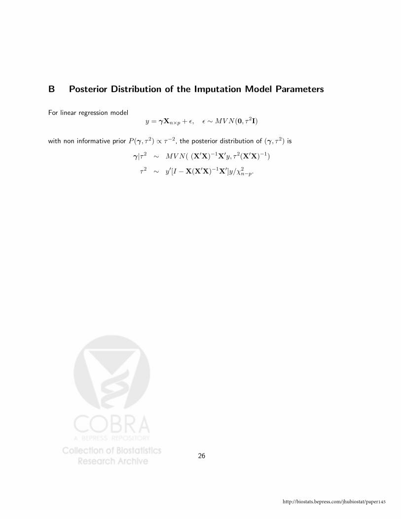
B Posterior Distribution of the Imputation Model Parameters

For linear regression modely = γXn×p + ε, ε ∼ MV N(0, τ2I)

with non informative prior P (γ, τ2) ∝ τ−2, the posterior distribution of (γ, τ2) is

γ|τ2 ∼ MV N( (X′X)−1X′y, τ2(X′X)−1)

τ2 ∼ y′[I −X(X′X)−1X′]y/χ2n−p.

26


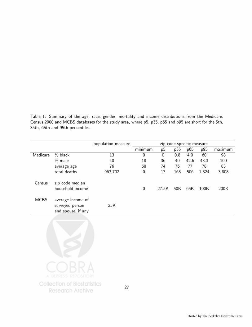
Table 1: Summary of the age, race, gender, mortality and income distributions from the Medicare,Census 2000 and MCBS databases for the study area, where p5, p35, p65 and p95 are short for the 5th,35th, 65th and 95th percentiles.

population measure zip code-specific measureminimum p5 p35 p65 p95 maximum

Medicare % black 13 0 0 0.8 4.0 60 98% male 40 18 36 40 42.6 48.3 100average age 76 68 74 76 77 78 83total deaths 963,702 0 17 168 506 1,324 3,808

Census zip code medianhousehold income 0 27.5K 50K 65K 100K 200K

MCBS average income ofsurveyed person 25Kand spouse, if any

27


Table 2: Estimates of Race Coeffcient, Population-Level AR, RAR and OR of Death Comparing Blacksversus Whites Adjusted for Income Using Logistic Regression Model (1) Without Random Effects, withIndividual-Level Income Imputed from Different Imputation Models (Selected Results of 5 out of 9imputation models).

Estse Model 1 Model 2 Model 5 Model 7 Model 9age age age age age

* race * race * race * race * race* gender * gender * gender * gender * gender

death death death death deathlog(incomez) log(incomez) log(incomez) log(incomez) log(incomez)

% blackz % blackz % blackz % blackz

log(%povertyz) log(%povertyz) log(%povertyz)log(%highz) log(%highz) log(%highz)

Other SESz

log(incomec) log(incomec)% povertyc % povertyc

highc % highc

Race coef −0.002.0184 0.025.010 0.030.007 0.026.014 0.035.010

AR −0.0002.0018 0.0026.0010 0.0031.0008 0.0027.0014 0.0037.0010

RAR −0.0035.0325 0.047.019 0.057.014 0.050.026 0.066.019

OR 0.9963.0344 1.050.020 1.060.015 1.053.028 1.070.020

z indexes zip code and c indexes county.

Other SESz includes zip code-level % degree completeness ,% public transportation, % house owner, % house

owner 65+, and% unemployment

28


Fig

ure

1:Loca

tion

ofth

e20

95zi

pco

des

incl

uded

inou

rst

udy

area

aswel

las

the

410

zip

codes

within

study

area

with

MCB

Sen

rolle

es.

within study area

MCBS enrollment

study area

29


Figure 2: Posterior Densities of Attributable Risk (AR), Relative Attributable Risk (RAR), and OddsRatio (OR) of Death comparing Blacks versus Whites, adjusted and not adjusted for income.

0.000 0.005 0.010 0.015 0.020

020

040

060

080

0

AR

NOT Adjusted for IncomeAdjusted for Income

0.00 0.05 0.10 0.15

020

4060

8010

012

0

RA

R

1.00 1.05 1.10 1.15 1.20

020

4060

80

OR

30


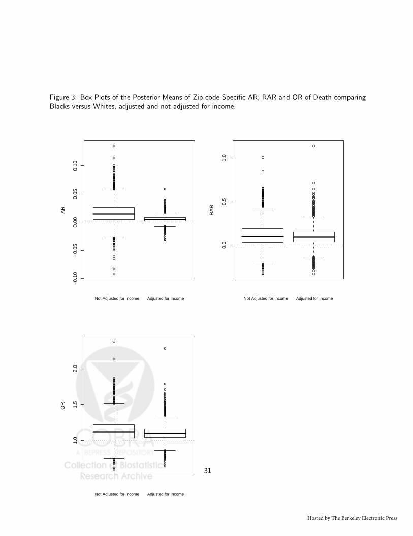
Figure 3: Box Plots of the Posterior Means of Zip code-Specific AR, RAR and OR of Death comparingBlacks versus Whites, adjusted and not adjusted for income.

−0.

10−

0.05

0.00

0.05

0.10

AR

Not Adjusted for Income Adjusted for Income

0.0

0.5

1.0

RA

R


1.0

1.5

2.0

OR


31


racial disparities in mortality risks in a sample of the …

Documents