race track optimizationdesigninformaticslab.github.io/_teaching/designopt/projects/2015/... · race...
TRANSCRIPT

Race Track Optimization 5/10/15
Team 3
Lucas Jaramillo
Fabian Gadau
Myrtle Lin
Bryce Thompson
Abstract
This design project will involve the optimization of the path a race car should take around
a given automotive race track to minimize its lap time. The scope of this project is to model the
most important subsystems of the car to predict its performance, after which it is possible to find
the quickest path around a given racetrack based on an optimal path, optimal velocity profile and
optimal user inputs. Comprehensive models of the subsystems will be used in order to constrain
the maximum possible positions, velocities, and accelerations of the car. These include the
incorporation of the vehicle’s dynamics, traction, and powertrain as well as the track’s geometry.
The goal of this project is to provide an optimal path with velocity and user input profiles that are
achievable for the car at each finite section of the track in order to minimize overall lap time. In
the end different plausible routes and velocities will be analyzed to find an optimum path by
applying true vehicle constraints, i.e. traction and dynamic limitations. The motivation of this
project is to apply these techniques to aid the development of the vehicles designed by students at
Arizona State University competing in the Formula Collegiate Design Competition hosted by the
Society of Automotive Engineers. This project will also benefit the amateur drivers who are
driving, so that they can be better prepared for competitive motor sports.

1
Table of Contents
1. Introduction ........................................................................................................................ 3
2. Problem Statement .............................................................................................................. 5
3. Nomenclature ...................................................................................................................... 6
4. Track Geometry .................................................................................................................. 8
4.1 Problem Statement ....................................................................................................... 8
4.2 Mathematical Model ..................................................................................................... 8
4.3 Model Analysis ............................................................................................................. 9
4.4 Optimization Study ......................................................................................................10
4.5 Parametric Study .........................................................................................................10
4.6 Discussion of Results ....................................................................................................10
5. Tire Pressure ......................................................................................................................13
5.1 Problem Statement ......................................................................................................13
5.2 Nomenclature ..............................................................................................................13
5.3 Mathematical Model ....................................................................................................13
5.4 Model Analysis ............................................................................................................15
5.5 Optimization Study ......................................................................................................16
5.6 Parametric Study .........................................................................................................17
5.7 Discussion of Results ....................................................................................................19
6. Vehicle Dynamics ...............................................................................................................20
6.1 Vehicle Dynamics Problem statement ...........................................................................20
6.2 Nomenclature ..............................................................................................................21
6.3 Mathematical Model ....................................................................................................23
6.4 Model Analysis ............................................................................................................24
6.5 Optimization Study ......................................................................................................25
6.6 Parametric Study .........................................................................................................26
6.7 Discussion of Results ....................................................................................................26
7. Power Train .......................................................................................................................28
7.1 Problem Statement ......................................................................................................28
7.2 Nomenclature ..............................................................................................................28
7.3 Mathematical Model ....................................................................................................29
7.4 Model Analysis ............................................................................................................32
7.5 Optimization Study ......................................................................................................32
2
7.6 Parametric Study .........................................................................................................35
7.7 Discussion of Results ....................................................................................................36
8. System Integration Study ....................................................................................................37
8.1 AIO Approach ............................................................................................................................ 38
8.2 Usability of Results and Future Work ..................................................................................... 40
9. References ..........................................................................................................................41
10. Appendix ........................................................................................................................42

3
1. Introduction
Following the most time efficient path a specific car can take around a real track can have a
substantial impact on the success of a racing team. The most straightforward method to winning
a race is to design the car that has the highest base performance figures and is tuned to the track
as well as the most talented and focused driver behind the wheel. In most cases this is not the
case and one has to make the best out of an imperfect situation.
The impact of these simulations can elevate the team above the competition. Every lap the race
car has to drive around the track is taxing on both the components of the car and the budget of
the team, so tuning a few of the car’s subsystems before a lap is ever driven on the track can
drive down the cost and work substantially. On the driver side, it is often difficult to quantify
how good a race driver is, as well as how to improve the performance of said driver other than
communicating that he should push harder in a certain sector. Knowing the ideal line, velocity
and inputs that the driver should make makes quantifying improvement suggestions simpler.
Because of the high number of subsystems and limited time and experience of the members of
this team, the scope of this project must be limited to a few of the most important subsystems of
the car.
The paper has a built model with 4 different subsystems to optimize the fastest lap time around a
track. The model will be divided into four subsystems:
1. Track Geometry
2. Tire Model
3. Vehicle Dynamics
4. Powertrain
To optimize the fastest race path and time, assumptions are made as follow:
1. The geometry is rigid.
2. The car travels within the upper bounds and lower bounds of the track.
3. The car has front wheel steering.
4. There is constant tire contact with pavement, so no tilt steering will happen.
Using these models and assumptions, a MATLAB tool will be created to determine the fastest
path around the track. The displayed output data will determine if it can be achieved and
controlled by a human driver.

4
Subsystems Considered
a. Track Geometry
To generate meaningful data from the track the real geometry of the track must be
available. The track will be generated in MATLAB with cubic spline function. Then the
initial path will be picked at random as long as it is within the lower bounds and upper
bounds. The different paths will give a derivative of time elapsed between points. The
different paths will vary due to the users speed, turn of the steering wheel, change the of
the gear, or a combination of the three. This result will be expanded with many options
over the course of the track and gives an estimate of the time required for one lap. The
model will use the power train, traction, and vehicle dynamics as well as static
environmental values to bind the possible options the user can take.
b. Tire Pressure
The Tire pressure model will take into account the speed of the vehicle at any given time
on the track. It will then combine that data with the pressure in the tires in order to
determine the frictional coefficient between the vehicle and the track. This frictional
coefficient will be used in the vehicle dynamics model in order to determine the
maximum speed at which the car can travel at any given point of the track, especially in
turns. This subsection will allow us to determine the optimal tire pressure by altering the
pressure in the tires and determining how it will effect lap times.
c. Vehicle Dynamics
The car can only handle a finite amount of angular acceleration before the driver is either
forced to break in a non-ideal location or lose traction. This occurs when the angular
acceleration of the car is greater than the amount of traction that the tires can handle. The
vehicle dynamics model relates the tire model, powertrain, and track geometry data in
order to determine the current information regarding the vehicle’s angular acceleration
into one single subsystem. Furthermore, this model optimizes the suspension stiffness in
order to lower the angular force seen on the tires, hence maximizing the powertrain
output by minimizing the resulting lateral forces seen as a steering byproduct.
d. Powertrain
To properly model the acceleration of the vehicle in the forward direction, powertrain
must be considered and modeled. We are using information such as the gear ratios, and
wheel size from the internet given the Subaru STi that we are using for testing. The
model optimizes the location of the gear changes, where to brake, and the throttle
position, to make sure the car can achieve the modeled velocities.
5
2. Problem Statement
There is a huge population interested in fast racing, but only one in millions make it to the fastest
race track. With the lack of experience and hands on application, many miss out on an
opportunity to drive like a professional. In order to be the fastest one around a race track, one
must have professional skills and experiences that help guide them through the process.
Professional racecar drivers make decisions based on intuition and experience to determine their
desired acceleration through turns and during straightaways.
Therefore, this model will allow inexperienced individuals to know the optimal path and places
for car adjustments to allow the fastest time around the race track with minimal racing
experience. By looking at the traction, vehicle dynamics, powertrain and the modeled track
geometry will allow users to know the best coefficients to use on their actual cars. The optimal
solution for the traction, vehicle dynamics, or powertrain may not be the optimal solution when
these four subsystems are put together.
A race track can be modeled in a two- dimensional model or three- dimensional model. For
simplification purposes, this model will first concentrate on a two-dimensional model. If time
permits, a three-dimensional model will be created to better mimic a true racing situation on a
race track.

6
3. Nomenclature
The nomenclature documented in this table is the overall nomenclature that will be used
throughout the entire project and is made up of all the individual subsection nomenclatures.
Some subsections have a larger nomenclature than others and maybe restated in the individual
subsection.
Symbol Definition [Unit]
Wt Vehicle Weight [lb]
ag Gravitational Constant [ft/s2]
Fn Normal Force (vertical) [lbf]
hs Sprung Weight Center of Gravity Height [in]
Zf Roll Center Height (Front) [in]
Zr Roll Center Height (Rear) [in]
pd Sprung Mass Weight Distribution from Front Wheels [%]
Ws Sprung Vehicle Weight [lb]
Kd Wheel Track [in]
Kf,r Spring Weight – Front, Rear [lbf/in]
Ff Frictional Force [lbf]
Fc Centripetal Force [lbf]
Ac Lateral Acceleration [in/s2]

7
M Roll Moment [in-lbf]
Fm Spring Force [lbs]
X Spring Compression due to Body Roll [in]
P Tire Pressure [psi]
V Velocity [mph]
µ Tire/Track Frictional Coefficient
t Time [s]
Vvd Velocity bound based on Vehicle Dynamics [kph]
Vmax Maximum Feasible Velocity [kph]
dt Δt based on distance velocity for step calculated [s]
dx Δx based on the path calculated [m]
gn Gear ratio []
ωmotor Rotations per minute of motor [rpm]
dtgc Time since gear change began [s]
pt Position Throttle [%]
Cu Gear change up procedure in progress [Boolean]
Cd Gear change down procedure in progress [Boolean]
rwheel wheel radius [m]
rtransmission transmission ration []
8
4. Track Geometry
4.1 Problem Statement
The goal is to optimize the fastest lap time and path with changing vehicle dynamics at each
position of the track.
Minimize: Lap Time
Subject to: Changing Velocities
The track geometry model incorporated the other subsystems before it could fully optimize the
lap time. The initial track set up help provided the track curvature and track coordinates for the
powertrain, tire model, and vehicle dynamics subsystem.
4.2 Mathematical Model
The consensus of the group was to first create a simple oval track. This was initially done
by plotting ellipses and using a finite element analysis approach. How the track geometry is
modeled in MATLAB is dependent on how each subsystem functions. With the change in how
the subsystems would want to vary the initial guess the simple oval track was modeled
differently in MATLAB.
The first path that was created was through a cubic spline by plotting 6 points. This track
was initially a test track. It allowed each subsystem to understand where there mistakes may be
in a less complex of a track. When this was done, the actual track (Musselman Honda circuit
track) was modeled from acquired data. This was initially done by getting an image from the
internet and modifying it so the image would only have the track that was run on. Then the
image was inverted and the boundaries were shown. From this, it was undetermined how to
acquire the function of the upper bounds and lower bounds of the track.
The next approach was to upload the image into Solidworks and get a good amount of
points from the track. This resulted in 27 x and y coordinates each for the upper and lower
bounds. This allowed the group to create gates between the track. With the points gathered, a
cubic spline was done to connect the points of the track. Then within MATLAB, a smoothing
function was done so the track would not be rigid. This was done by matching the first and
second derivatives with the first and last point of the track. When the track was done being
inputted, modifications were done to eliminate oddly shaped corners. Shown below is the final
track with the gates created.

9
Figure 4.2.1 Track Geometry
Overall, instead of using a finite element approach, an angular cubic spline approach was
taken. By taking a cubic spline approach, there will be infinite paths for the car to travel within
the bounds of the track that can be easily evaluated using the gradient method. The cubic spline
outputs points for the upper bounds and lower bounds of the track. When the initial guesses and
changes to the guesses are taken, points will also be outputted and given to the remaining
subsystems.
4.3 Model Analysis
Constraints on the path of the car was that it must travel within the upper bounds and lower
bounds of the track. Of course, the upper bounds and lower bounds of the track cannot be
achieved when the actual car is racing, so an inequality constraint was done to have the car be
greater than the lower bounds but less than the upper bounds. With the created gates in our track,
the lower bound was able to be assigned when lambda was zero and the upper bounds was when
lambda equaled one.

10
The initial guess was the center of the track and lambda equaled 0.5. After the initial guess the
information was passed through the various subsystems and given back to the track geometry.
The track geometry path changed between iterations to find the fastest velocities at each point
which will correlate to the fastest time. The inputs of the system will be given from the
designers.
4.4 Optimization Study
The optimization of time could not have been acquired until the powertrain, tire model, and
vehicle dynamics section was running. The initial optimization problem was going to be done
through fmincon, but since the function of the track was never defined as a regular function it
caused complications. The purpose of these created gates was that it estimated the next path
between gates. As the estimated path changed, the gradients from one gate to another changed as
well. This allowed the team to find the different times as the path slightly changed. A gradient
method and Armijo Linesearch were implemented into the code to find the fastest overall lap
time through these gates. Since the track data implemented a gradient function for the gates,
Linesearch was also implemented using the gradient function. Linesearch ensured that the time
found was less than the time found through the gradient method. If this was not done, then the
initial alpha (step direction) was cut in half.
4.5 Parametric Study
The optimum lap and time changes as the upper and lower bound parameter changes. The length
and complexity of the track also effects the lap time. The optimization will take longer with a
more complex track because there will be more gear and velocity changes. Therefore, results
cannot be generalized since they are dependent on how the track is outlined. At the same time,
ranges of parameter values cannot be predicted for any solution. Shown below are results from a
simplified track and in future sections results from a more complex will be shown and discussed.
4.6 Discussion of Results
The optimization of all the codes together was first done to a simplified track. The sampled
racing lines shown below could only be realistic racing lines. Below are results from the
simplified model to ensure that the complied codes worked.

11
Figure 4.6.1 Sampled Racing Lines
The simplified track only had 6 gates. Below the optimization results show how the implemented
gradient method and Linesearch affected the lap time with every iteration.
Figure 4.6.2 Optimization Results
-1000 -500 0 500 1000 1500-800
-600
-400
-200
0
200
400
600
800

12
The paths were usually bounded by the track or powertrain. Two local solutions were able to be
found. Path one took 62.6 seconds and ran along the outside of the track. While path two took
64.2 seconds and ran on the inside of the track.
Figure 4.6.3 Path 1 Results
Figure 4.6.4 Path 2 Results
These two local solutions are expected racing lines that could happen. These path data will allow
a driver to know the fastest way around a track or the best way to surpass someone on the track.
The solution accounts for shifting gears, full throttle, and is limited to the vehicle dynamics.

13
5. Tire Pressure
5.1 Problem Statement
When attempting to optimize the time it takes a car to go around a track it becomes very
important to look at what kind of traction the tires will have on the pavement. The traction
ultimately determines the speeds that the car can handle while going around a track. Before a
race starts tire pressure is one of the few things that can be adjusted in order to best help with
how a car rides and the traction it makes with the track. Traction is typically higher at low speeds
with higher tire pressure and higher at high speeds with low tire pressure. So depending on track
dimensions and the speed ranges at which the car will travel different pressures will be better or
worse. In this subsystem we will create a model that outputs a tire/track frictional coefficient for
all possible velocities with a given tire pressure. Currently there are no working mathematical
models that we are aware of that perform this function. We will be using data collected by The
Department of Motor Vehicles to create a META model that we can then integrate into the rest
of the subsections in order to get the fastest lap times.
5.2 Nomenclature
Symbol Quantity Unit
P Tire Pressure [psi]
V Velocity [mph]
µ Tire/Track Frictional Coefficient
t Time [s]
5.3 Mathematical Model
Objective Function
The goal of this subsection is to find the optimal tire pressure that can be used in the tires in
order to minimize the time it takes for the car to travel around the track. In order to find the
optimal pressure all the other subsystems will need to be used. This subsystem will vary the
pressure and use a set of velocities around the track to find track times for each tire pressure and
then select the pressure that results in the fastest lap time.
Minimize: t=f (P, 𝑉)
14
Constraints
Physical Constraints
The tire pressure is naturally constrained by how much pressure a tire can safely hold. For this
model we used data from The Department of Motor Vehicles so I have chosen then upper and
lower bounds for tire pressure to match the max and min pressure tested in that data. These
constraints are denoted by G1 and G2.
𝐺1 = 17 − 𝑃 ≤ 0
𝐺2 = 𝑃 − 35 ≤ 0
Engineering Constraints
The other constraints to take into account are the max and min velocities at which the car can
travel at while going around the track. We can assume that the car will never go in reverse so we
set the lower bound for velocity at zero. The upper bound for velocity is to be determined by the
other subsystems and the mechanics of the vehicle. These constraints are denoted by G1 and G2.
𝐺3 = 𝑉 − (𝑇𝐵𝐷 𝑀𝐴𝑋 𝑉𝐸𝐿𝑂𝐶𝐼𝑇𝑌) ≤ 0
𝐺4 = −𝑉 ≤ 0
Summary Model
In summary the two part goal to this subsection is first to work with the other sections in the
overall model and to provide frictional coefficients that will be used with the vehicle dynamic
section. The second part of the goal will be to be able to optimize tire pressure for a track in
order to determine the optimal tire pressure that will provide the fastest possible lap times.
Minimize: t=f (P, 𝑉)
Subject To:
𝐺1 = 17 − 𝑃 ≤ 0
𝐺2 = 𝑃 − 35 ≤ 0
𝐺3 = 𝑉 − (𝑇𝐵𝐷 𝑀𝐴𝑋 𝑉𝐸𝐿𝑂𝐶𝐼𝑇𝑌) ≤ 0
𝐺4 = −𝑉 ≤ 0
15
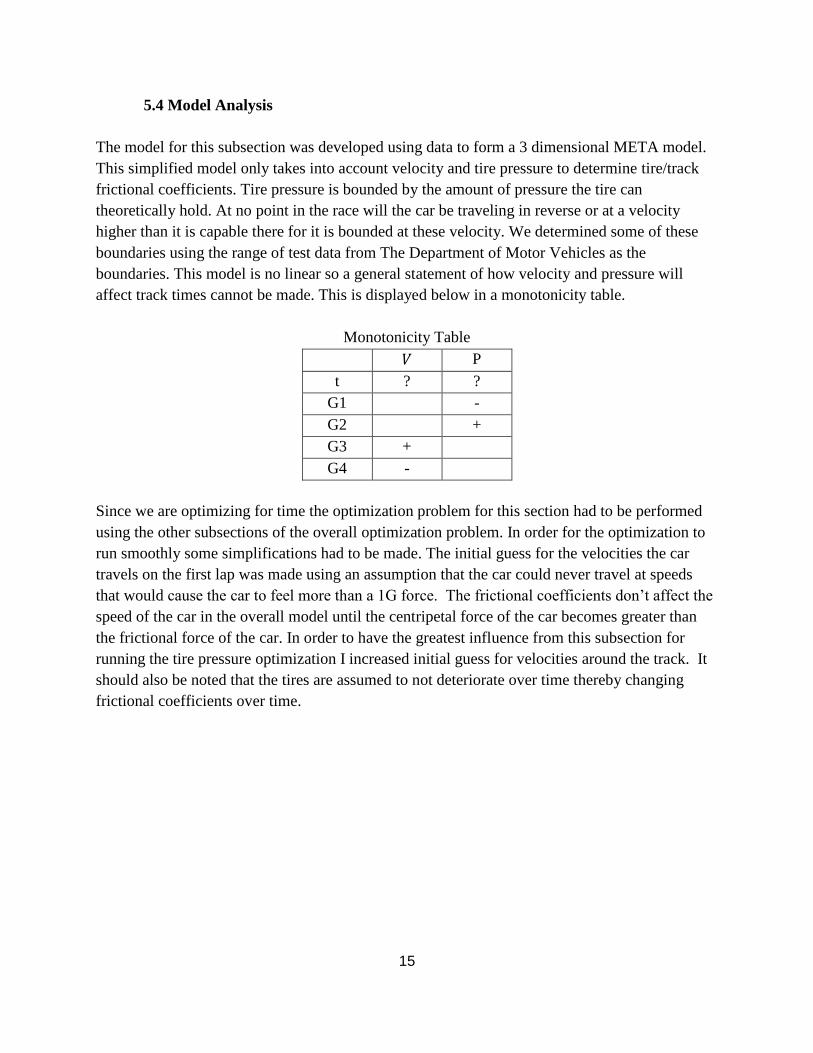
5.4 Model Analysis
The model for this subsection was developed using data to form a 3 dimensional META model.
This simplified model only takes into account velocity and tire pressure to determine tire/track
frictional coefficients. Tire pressure is bounded by the amount of pressure the tire can
theoretically hold. At no point in the race will the car be traveling in reverse or at a velocity
higher than it is capable there for it is bounded at these velocity. We determined some of these
boundaries using the range of test data from The Department of Motor Vehicles as the
boundaries. This model is no linear so a general statement of how velocity and pressure will
affect track times cannot be made. This is displayed below in a monotonicity table.
Monotonicity Table
𝑉 P
t ? ?
G1 -
G2 +
G3 +
G4 -
Since we are optimizing for time the optimization problem for this section had to be performed
using the other subsections of the overall optimization problem. In order for the optimization to
run smoothly some simplifications had to be made. The initial guess for the velocities the car
travels on the first lap was made using an assumption that the car could never travel at speeds
that would cause the car to feel more than a 1G force. The frictional coefficients don’t affect the
speed of the car in the overall model until the centripetal force of the car becomes greater than
the frictional force of the car. In order to have the greatest influence from this subsection for
running the tire pressure optimization I increased initial guess for velocities around the track. It
should also be noted that the tires are assumed to not deteriorate over time thereby changing
frictional coefficients over time.

16
5.5 Optimization Study
The optimal tire pressure was found to be 20.7 PSI both graphically and using Matlab’s built in
fmincon function. Once all the subsections were put together for the overall optimization I was
able to vary the tire pressure on a set path around the track and examine how it affected track
times. Figure 5.5.1 below displays the path that was used for this optimization.
Figure 5.5.1
The path follows closely around the inside of the track since I eliminated the 1G initial
assumption used for the velocities as I mentioned in the model analysis section. Using this path
and by varying the pressure in the tires from 17 psi to 35 psi I collected data on the time it takes
to complete a single lap on the track. Figure 5.5.2 displays the data collected during this process.

17
Figure
Figure 5.5.2 Results from Optimization
These results were then verified using Matlab’s built in fmincon function with various initial
guesses. Table 5.5.1 shows the results using fmincon.
Initial Guess (psi) Pressure (psi) Lap Time (Seconds)
17 20.6954 51.9568
26 20.6953 51.9568
35 20.6957 51.9568
Table 5.5.1 Results from fmincon
5.6 Parametric Study
As I ran the tire pressure optimizations one of the biggest parts of the code that had to be
adjusted was the part that guessed the initial velocities based on G-force as discussed. For the
solution found above I scaled the guess by a factor of 10 but to avoid extreme velocities I set a
limit on the upper bound for velocities of 80 mph. I kept the 80 mph cap for all my tests but I
adjusted the scaling factor I used from 1 to 10. When I scaled the initial velocities by anything
lower than 10 it resulted in flat spots on the graph. Figure 5.6.1 is the graph for when I used a
scaling factor of 8.

18
Figure 5.6.1 Data with Scaling factor of 8.
This data didn’t allow for a good optimization to be found. The graphs also became more flat
with lower scaling factors. This is due to the low initial guess for velocities. At low speeds the
centripetal force is never greater than the normal frictional force of the car and so the velocity of
the car is never limited by the frictional force and thus pressure would have no effect on lap
times. When these flat spots occurred fmincon would always give different optimal pressures
depending on the guess used with the fmincon function. Table 5.6.1 displays the results for
various scaling factors.
Optimal Tire Pressure
Scaling Factor Fmincon w/
Guess of 35 psi
Fmincon w/
Guess of 35 psi
Fmincon w/
Guess of 35 psi
Graphically
10 20.6957 20.6953 20.6954 20.7
8 33.9244 26 18.2575 17.5
6 34.01 26 17.99 33.6
4 34.01 24.2454 20.5319 31.8-35
2 34.01 26 17.99 17-35
1 34.01 26 17.99 17-35
Table 5.6.1 Results with Various Scaling Factors

19
5.7 Discussion of Results
The result of 20.7 psi found from this optimization is largely due to the track geometry we used
for this model. These results cannot be used as a generalization for tire pressure in any given tire
on any given track. It is assumed that if we were to use data from a different tire the results
would be different. Since the optimal tire pressure found did not occur at the boundaries it cannot
be simply stated based on this optimization that a lower tire pressure is generally better than a
higher pressure or vice versa. The solution of 20.7 psi makes sense for this car, with these tires,
on this track since it fell within the constraints of problem. In order to improve the solution
found we could reassess how we set the initial guess for velocities around the track. The model
could also be made much more complicated by not just looking at the lateral frictions but also
the friction in the longitudinal direction and how it would be integrated with the power train
model.

20
6. Vehicle Dynamics
6.1 Vehicle Dynamics Problem statement
To optimize the spring stiffness of the test vehicle based on the optimized projectile path and
velocity profile.
The vehicle dynamics model plays distinct roles throughout the course of the project. During the
initial phases of the racetrack path optimization, the vehicle dynamics model serves as a series of
physical relationships which calculates the highest attainable instantaneous velocity based on the
path curvature, estimated projectile velocity and tire pressure along with the corresponding
frictional coefficient between the tires and the pavement. Throughout this portion of the vehicle
dynamics model, the spring stiffness is set to the current actual value of that of the actual test
vehicle. Once the projectile path has been optimized, an independent optimization study is
performed on the vehicle dynamics model which is constructed of slightly more complex
relationships which describe the body roll and allow the spring coefficients to be treated as the
design variables. This model is described in detail throughout the following sections.

21
6.2 Nomenclature
Symbol Definition [Unit]
Wt Vehicle Weight [lb]
ag Gravitational Constant [ft/s2]
Fn Normal Force (vertical) [lbf]
hs Sprung Weight Center of Gravity Height [in]
Zf Roll Center Height (Front) [in]
Zr Roll Center Height (Rear) [in]
pd Sprung Mass Weight Distribution from Front Wheels [%]
Ws Sprung Vehicle Weight [lb]
Kd Wheel Track [in]
Kf,r Spring Weight – Front, Rear [lbf/in]
Ff Frictional Force [lbf]
Fc Centripetal Force [lbf]
Ac Lateral Acceleration [in/s2]
M Roll Moment [in-lbf]
Fm Spring Force [lbs]
X Spring Compression due to Body Roll [in]
Θ Body Roll [Degrees]
Fs Side Wheel Force [lbs]
V Velocity [ft/s]
hrm Sprung Weight Moment Lever Arm [in]

22
Fm Spring Force [lbs]
D Distance from updated Center of Gravity to Wheel [in]
R Turn Radius [ft]
𝐴𝑐 =𝑣
𝑟 ∗ 𝑎𝑔 (1)
ℎ𝑟𝑚 = ℎ𝑠 − (𝑍𝑓 − (𝑍𝑟 − 𝑍𝑓)(1 − 𝑝𝑑) (2)
𝑀 = ℎ𝑟𝑚𝑊𝑠𝐴𝑐 (3)
𝐹𝑚 = 𝑀
ℎ𝑟𝑚
(4)
𝑥 = 𝐹𝑚
2𝐾
(5)
θ = 𝑡𝑎𝑛−1 (𝑥
ℎ𝑟𝑚)
(6)
d = 𝐾𝑑
2− 𝑥
(7)
𝐹𝑠 = 2𝑀
𝑑
(8)
𝐹𝑓 = 𝜇𝐹𝑛 (9)
𝐹𝑐 = 𝑊𝑡
𝑎𝑔 (𝑣2
𝑟 )
(10)
𝑣 = √𝜇𝑎𝑔𝑟 (11)
F = (𝑘𝑓+𝑘𝑟)𝑥2
2
(12)

23
6.3 Mathematical Model
The goal of the vehicle dynamics model is to study the motion of the vehicle throughout the
projected path and to calibrate and optimize the suspension stiffness that will best suit the
vehicle’s body roll according to the nature of the vehicle’s route and inputs. In other words,
finding the optimal front and rear spring coefficients in equation (12), namely Hooke’s Law.
Mathematically, the vehicle dynamics system has three major system constraints, consisting of
the tire traction, body roll and available suspension travel, pertaining to equations (9), (6) and
(5), respectively. Refer to appendix for model modifications.
The vehicle dynamics simulation
subsystem model essentially studies
the lateral forces involved with the
vehicle’s motion. Due to a lack of
testing instrumentation, this model
strictly relies on physical models
which determine the leading factors
that directly impact the velocity of the
projectile. The simulation portion of
the vehicle dynamics model takes into
account the initial vehicle velocity
guess, tire pressure, frictional
coefficient between the pavement and
tires along with the curvature of the
track in order to calculate the
maximum achievable velocity throughout the given corner.
Furthermore, the simulation subsystem provides the optimization model with more detailed
physics which provide the necessary information to accurately model the suspension parameters
[kf kr]. An important concept to note for this section is that the vehicle was modeled as a
spring/mass system for convenience; A true vehicle dynamics model is much too complex for
this level of analysis required for this subsection, which would realistically involve time
dependent fluctuations in the spring/damping system, heat transfer and fluid viscosity
calculations, mass transfer along with other high order differential equations. For the purpose of
this report, the essential physical relationship involved in this subsystem is to track the motion of
the swaying center of gravity. Based on the true vehicle geometry, a simple mass and spring
model was formulated in order to approximate the forces involved with the vehicle’s body
motion, which rotates around a “roll axis”. This rotation produces a centripetal force that results
directly upon the tires, which are bounded by the tire traction model’s predicted frictional
24
coefficients. The model then sums the forces which act upon the tire, causing an increase in tire
pressure, hence a variation in frictional coefficient, along with the forces seen by the suspension
components in order to perform the system’s optimization task.
To summarize, the vehicle dynamics model plays two major roles. The simulation role corrects
the predicted cornering velocity by inputting the variables V, P, 𝜇 and r (velocity, pressure,
frictional coefficient and track curvature) and outputs the corrected cornering velocity, V. The
true mathematical model for the optimization procedure takes in the resultant forces from the
constrained simulation model and optimizes the spring stiffness coefficients.
6.4 Model Analysis
As mentioned in the previous section, the system’s model is substantially simplified by
describing the vehicle’s lateral motion via spring and mass relations. A few of the major
assumptions which simplified the physics involved can be found below.
o No dampening effects – No fluid, heating nor time dependence involved in the
suspension.
o Tire forces only account for an increase in tire pressure – No change in contact
area nor heating effects.
o Immediate body mass response – This eliminates any time dependent or force
memory involved in the body sway.
o No rotational momentum storage as the inflection point varies.
o Tire sliding is not achievable (This point acts as a model constrain).

25
6.5 Optimization Study
The optimal spring rates shown below are the results which were achieved by fitting the
suspension reactions as the vehicle underwent turns, to the actual suspension geometry. This was
performed by essentially fitting all of the individual suspension travel readings (forces pertaining
to 2001 points) into Hooke’s model while allowing the suspension stiffness to be variable, in
order to avoid full suspension compression. This task was performed by using a user defined
gradient step method.
Figure 6.5.1 Local minima solutions to Hooke’s model. The plot shows the front and rear spring
stiffness combinations that work with the given projectile path and forces seen on the suspension
to avoid bottoming out the suspension travel and absorb the majority of the energy involved in
the body motion.
In order to create more interesting results, the body weight distribution was varied over different
optimization runs; the numbers seen in the legend correlate to the front/rear vehicle weight
distribution.

26
6.6 Parametric Study
The model converged on various local minima as the initial guess points were varied. The
following table provides the results from the variation for the common 65% front, 35% rear
weight distribution analysis.
Distribution Initial Guess k1 k2
65/35 70/70 408.82 252.45
65/35 100/150 382.17 301.94
65/35 80/80 406.89 256.02
65/35 10/50 403.69 261.99
65/35 25/125 375.75 313.87
65/35 125/50 429.53 213.98
65/35 50/50 412.67 245.29
65/35 100/100 403.05 263.18
65/35 80/135 383.94 298.66
Table 6.6.1 Local minima achieved as the result of initial guess variation. Note that some of the
initial guesses result in a duplicated local minima.
Due to the linear relationship seen in the spring stiffness solutions, the feasible solutions are
fairly predictable. This predictability makes sense given that if the spring rate is relaxed on one
side of the vehicle, the opposite will require a higher spring rate in order to effectively absorb the
energy produced throughout the cornering process, providing a linear range of feasible solutions
to each vehicle weight configuration.
6.7 Discussion of Results
The results of the optimization study are slightly higher than the actual spring rate found in
the modeled vehicle (220 lbf/in front and 185 lbf/in rear) which is mostly due to the over
simplification of the physical process that truly occurs in a vehicle. The trends make perfect
sense and the graph below will provide further insight to these numerical values.

27
Figure 6.7.1 Shows the total theoretical suspension travel seen by model throughout the
course of the track. The suspension travel is calculated from the body roll force and
momentum equations.
The true suspension of the vehicle has a total of 6.00” inches of travel, of which 2.75” are
consumed by the sprung weight of the vehicle, leaving 3.25” of available spring travel to
absorb energy throughout the cornering process. The red portion of the graph suggests that
the original suspension stiffness experienced loads that were too high to handle, which in
practice would cause the suspension to bottom out and send the force to the tire, which
essentially works against the grip and causes premature sliding.
The optimization model takes these forces into account and optimizes the coefficient so that
the suspension is will never bottom out throughout the course of the projectile, hence the
higher spring coefficient values. Any of the local minimum solutions that are shown in table
6.6.1 are acceptable values for the current global system.
28
7. Power Train
In many cases optimizing the powertrain is an extremely costly endeavor that requires
testing, manufacturing or control system knowledge. In this sub problem the focus of the
optimization was therefore how the user (driver) interacts with the car. This allows a
support team to give precise feedback to the driver to give him the best chance to beat
the competition.
7.1 Problem Statement
Optimize the user interactions with the powertrain such as gear change timing, throttle
position and brake pedal position to minimize lap times based on a predetermined path
around a track.
7.2 Nomenclature
Symbol Definition [Unit]
Vvd Velocity bound based on Vehicle Dynamics [kph]
Vmax Maximum Feasible Velocity [kph]
dt Δt based on distance velocity for step calculated [s]
dx Δx based on the path calculated [m]
gn Gear ratio []
ωmotor Rotations per minute of motor [rpm]
dtgc Time since gear change began [s]
pt Position Throttle [%]
Cu Gear change up procedure in progress [Boolean]
Cd Gear change down procedure in progress [Boolean]
rwheel wheel radius [m]
rtransmission transmission ration []
29
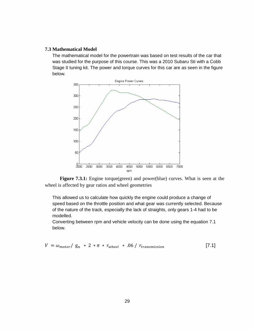
7.3 Mathematical Model
The mathematical model for the powertrain was based on test results of the car that
was studied for the purpose of this course. This was a 2010 Subaru Sti with a Cobb
Stage II tuning kit. The power and torque curves for this car are as seen in the figure
below.
Figure 7.3.1: Engine torque(green) and power(blue) curves. What is seen at the
wheel is affected by gear ratios and wheel geometries
This allowed us to calculate how quickly the engine could produce a change of
speed based on the throttle position and what gear was currently selected. Because
of the nature of the track, especially the lack of straights, only gears 1-4 had to be
modelled.
Converting between rpm and vehicle velocity can be done using the equation 7.1
below.
𝑉 = 𝜔𝑚𝑜𝑡𝑜𝑟/ gn ∗ 2 ∗ 𝜋 ∗ 𝑟𝑤ℎ𝑒𝑒𝑙 ∗ .06 / 𝑟𝑡𝑟𝑎𝑛𝑠𝑚𝑖𝑠𝑠𝑖𝑜𝑛 [7.1]
30
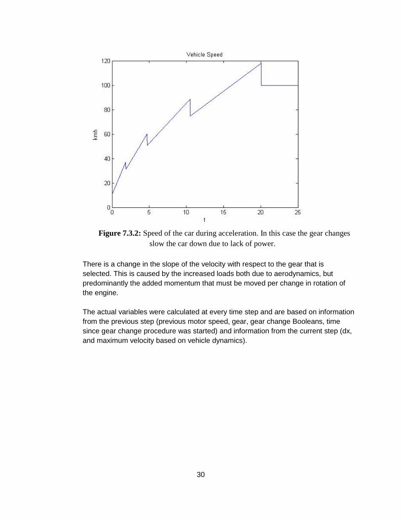
Figure 7.3.2: Speed of the car during acceleration. In this case the gear changes
slow the car down due to lack of power.
There is a change in the slope of the velocity with respect to the gear that is
selected. This is caused by the increased loads both due to aerodynamics, but
predominantly the added momentum that must be moved per change in rotation of
the engine.
The actual variables were calculated at every time step and are based on information
from the previous step (previous motor speed, gear, gear change Booleans, time
since gear change procedure was started) and information from the current step (dx,
and maximum velocity based on vehicle dynamics).

31
The Initial guess on user interactions is based on output from a flowchart as seen
below:
Figure 7.3.3: This simplified flowchart shows the algorithm that was used to
create an initial guess for user interactions with the powertrain for each step.
The above initial guess algorithm created a few problems. The first of which was
that in situations where the VD bound on Velocity decreased fast enough to where
even breaking was not able to keep it inside the vehicle dynamic bounds. This

32
was solved using a backtracking method that changed previous steps needed to
comply with the VD bounds. This is extremely important as it ensures a viable
situation based on the model.
The other problem was that the model sometimes quickly oscillated between two
gears. This was solved by taking out gear changes that oscillated between two
gear changes after the first change, if they happened quickly enough. This
heuristic change made a huge impact on lap times.
7.4 Model Analysis
This model is an extremely simplified model of a drive train. This was done because
we wanted to capture enough of the drive train characteristics to give a feasible
solution, but spend the majority of the time focusing on optimization strategies.
At each step the model can either be bounded by the Vehicle Dynamic model or the
Powertrain model or in many cases both. Formulated in a different way, the
achievable velocity is bounded by the fact that the car can’t go around corners at any
speed, or that motor can’t accelerate fast enough. Also, the car can be bound by both
at the same time. This happens when the user has to place the throttle between 0 and
100%. These driving situations are the most difficult for the driver, because he has to
keep track of two bounds. It is in these sectors that the most time can be gained.
7.5 Optimization Study
To optimize the location of gear changes, the initial guess was based on the fastest
feasible path around the track, which already included the lack of false oscillations of
the gear changes.
The location of the gear changes were moved in either direction until a minimum time
was found. To achieve this I chose to use a gradient based method. This was done
by calculating the time around the entire track based on having a specific gear
change in the original location, as well as having it in the location one step prior and
one step later than the original.
If either the earlier or later gear changes were faster than the original one, then that
one was chose as the new central location. This was repeated until the central
location was faster than the two adjacent. In almost all locations a few shifts were
made. This can be seen in the next table.

33
Table 7.5.1: Gear Change Optimization Results
Gear Change
Number
Number of Steps
Shifted
Time Advantage (s)
(+) is good
1 3 0.0311
2 0 0
3 2 0.0481
4 9 0.0789
5 1 0.0016
6 3 0.0027
7 0 0
8 0 0
9 3 0.0079
10 6 0.0634
11 7 0.0328
12 4 0.1085
13 0 0
14 6 0.0105
15 3 0.0232
16 3 0.0551
17 1 0.0013
18 0 0
19 0 0
20 3 0.7784
21 0 0
22 0 0
23 1 0.1546
24 0 0
25 2 0.0321
26 0 0
27 0 0
28 2 0.0555
29 2 0.0958
30 1 0.0044
31 2 0.0208
32 0 0
33 3 0.0126
34 1 0.1232
35 1 0.0009
36 0 0
37 2 0.0042
38 2 0.0027
39 1 0.0003

34
Figure 7.5.1: Time gained by optimizing gear changes compared to the initial
guess
Figure 7.5.2: Vbounds based on Vehicle Dynamics (green) and actual velocities
(red) during the race as well as the gears (black) at that location.
0 10 20 30 40 50 60 70 80 90 100-1.8
-1.6
-1.4
-1.2
-1
-0.8
-0.6
-0.4
-0.2
0
0.2Time Increase vs IG over the course of the race
% race completed
t(s)
0 10 20 30 40 50 60 70 80 90 1000
20
40
60
80
100
120
140

35
Figure 7.5.2: Gear Changes Optimization results.
7.6 Parametric Study
There are two major bounds to the powertrain model that increased the performance of
the vehicle.
The first is the maximum rpm of the engine. In this case the engine is limited by the ECU
to 7000 rpm. This is quite common for normal consumer engines, and the parts are
made to last at the loads experienced here for the lifetime of the engine. If the
components are upgraded, this number can be increased. A 100 rpm increase makes
the lap 0.3146 second faster. This is why formula one and performance motorcycle
engines operated in the 12-20 krpm range.
Second, increasing the throttle response increases the lap times. This can be achieved
by reducing the weight of the components that are used inside of the engines, as they
prevent the fast changes in rpms.
The results of the parametric study can be seen below.
Action Result
Max. Rpm 7100 vs 7000 -0.3146 s/lap
Increasing throttle response by 1% -0.0568 s/lap
0 10 20 30 40 50 60 70 80 90 1001
1.2
1.4
1.6
1.8
2
2.2
2.4
2.6
2.8
3Gear Changes vs % completed
% race completed
t(s)
optimized
IG

36
7.7 Discussion of Results
The problem statement has been met. A model that predicts the performance of a
powertrain and how it behaves with the user inputs has been created.
More importantly, after the initial guess was made a faster solution can be found by
changing the location of the gear changes. This is especially efficient for race day
applications, as there are few if any parametric changes that can be made on race
day to change the performance of the vehicle. Those slight changes can have a
profound impact on the race results as 1.7 advantages per lap are immense. In most
scenarios this is enough to lap the competition, or keep up with much more
expensive cars.
On another note, as the parametric study shows, changing physical components of
the car can also have an effect on the performance. More importantly, this model can
be used to predict the effect that a physical upgrade can have on lap times. This
makes picking out components for engineers much simpler. Especially when budget
is a limiting factor and one has to change between different options.
Lastly, the engine can undergo testing in a lab setting that mimics what is to be
expected during a race. This can be used to stop the engine from creating
unexpected problems during the race.
Opportunities for a better model are outlined below.
Model the control system of the car used for throttle response
Model the turbo, especially turbo lag at low rpms.
Optimize the physical components to increase lap times
o This is especially true of the gear box, which could be tuned for the
specific race track.
Increase the steps between states especially in areas that are important, such as
when there are gear changes.

37
8. System Integration Study
To create viable results for the optimized times for the racetrack, the four basic models of
the car have to be able to work well together.
Since the way data was transferred between the models was quite complex, this process is
bets followed using a flow chart.
An initial guess is made. To
save computation time, this
was an expected racing line.
The path is then created
using methods outlined in
section 4. The tire friction
are then calculated based on
velocity estimates based on
the curvature, this is outlined
in section 5. These tire
friction at every point are
then sent to the vehicle
dynamic model. This outputs
velocity bounds at every
point. These bound are then
passed to the powertrain
which optimizes the gear
changes to minimize the
time around the track. The
gradients are then calculated
by varying the track
geometry at every gate
minutely and then storing
that difference. The gates are
then moved to minimize the
time around the track. The
step size is controlled by the
Armijo line search. This is
repeated until a time is found
that is faster than the guess
at the beginning of each step.
This is terminated once a local minimum is found. This is determined when an extremely
small change in gates in the direction of the gradient produces no advantage.

38
8.1 AIO Approach Finally, our optimization achieved real, realistic results. For the path, the results
showed that in certain sectors the curvature was minimized, in others the shortest
path was taken. This is especially apparent in turn 1. To maximize curvature the turn
could have been taken slightly wider. This however increased the distance, which
increased the race time.
Figure 8.1.1: Outline of the best local minimum.
Discussion: This was found based on an initial guess that was close to a racing line. The result
was ~5 seconds faster than the best solution by hand. This is very close to an accepted ‘racing
line.’ This solution is affected by the location of the gates. The solution can change based on
where they are.
0 200 400 600 800 1000 1200 1400 16000
100
200
300
400
500
600
700
800
900
1
Track Path Optimization Result

39
Figure 8.1.2: Plot of the convergence of the racing line on a local solution.
Discussion: The initial guess was as close to a racing line as possible by hand and experience.
The search was terminated after 50 iterations based on the convergence criteria, that the Armijo
line search failed to reach a better solution.
5 10 15 20 25 30 35 40 45 50
120
125
130
135
140
145
Convergence Plot
Lap
Tim
e (
s)
Iteration Number

40
Figure 8.1.3: Plot of the convergence of the racing line on a local solution. The green line is the
Vehicle Dynamic Bound, the red line is the achievable velocity, and the black line is the gear at
each point.
Discussion: This profile shows the distribution of the velocities around the track. In most cases
this is bounded by the vehicle dynamic bounds. However when it isn’t the effect of full being at
full throttle can be seen. The gear changes appear feasible across the board, and don’t oscillate.
8.2 Usability of Results and Future Work The racing line results are much better than expected at the beginning of the project. More
options should be considered by changing the locations of the gates.
The results for the gear changes are all dependent on the powertrain, which, as it wasn’t the
focus of this study, could have been better. To turn this into a usable model the following should
be done. Create and validate good models of the car. Incorporate surface conditions such as
temperature, roughness, wetness and elevation of the track. If these are correct this could be a
very useful tool.
0 10 20 30 40 50 60 70 80 90 1000
20
40
60
80
100
120
140V
elo
city (
km
h)
/ g
ear
(#)
Track Completed (#)
Velocity and Gear Profile over race

41
9. References
C.H.A. Criens, T. ten Dam, H.J.C. Luijten, T. Rutjes, Building a MATLAB based Formula
Student Simulator. Technische Universiteit Eindhoven. June 20, 2006
D Bastow. “Car Suspension and Handling, 2nd edition”. In: SAE (1987).
David A. Crolla. “Automotive Engineering” Powertrain, Chassis System and Vehicle
Body””. In: Automotive Engineering (2009), pp. 107–125.
Honda R&D America, Vehicle Dynamics and Simulation “Vehicle Dynamics Simulation for
Predicting Steering Power-Off limit Performance”. SAE International 2008.
John B. Heywood. “Internal Combustion Engine Fundamentals”. In: Mechanical Engineering
(1988), pp. 49–55.
Rajesh Rajamani, Vehicle Dynamics and Control. University of Minnesota 2006.
Thomas D. Gillespie. “Fundamentals of Vehicle Dynamics”. In: Society of Automotive
Engineers, pp. 79–120.
Ying Xiong, Racing Line Optimization. Massachusetts Institute of Technology. September
2010.
Jones, D. R., C. D. Perttunen, and B. E. Stuckman. "Lipschitzian Optimization without the
Lipschitz Constant." Journal of Optimization Theory and Applications 79.1 (1993): 157-81.
Venkataraman, P. Applied Optimization with MATLAB Programming. New York: Wiley,
2002. Print.
MacIsaac J., & Riley G. (2002). Preliminary Findings of the Effect of Tire Inflation Pressure
on the Peak and Slide Coefficients of Friction. Report No.: DOT HS 809428. United States.
US Department of Transportation.

42
10. Appendix
10.1 Vehicle Dynamics Modifications
The vehicle dynamics model was completely modified from the original method of analysis.
Originally, our global system was to be modeled using a finite element method, in which the
total accumulated force was to be calculated at each point and decide how the next integration
point would affect each decision to be made. In order to accurately model the vehicle dynamics
for this original idea was to focus heavily on the tire forces, which included steering angle, front
tire turning modeling, power delivery, contact area size, immediate pressures and force history.
The original system of equations took all of these subsystems into account and was to be
modeled as the link between the tire and powertrain analysis to the track geometry. The
equations to be used for the original can be found in section 10.2
10.2 Original Vehicle Dynamics Model (Suspension)
Nomenclature:
lf Longitudinal Distance from C.G. to Front Tires [m]
lr Longitudinal Distance from C.G. to Rear Tires [m]
Ψ Yaw [m]
m Mass [kg]
δ Steering Angle [degree]
𝜔w Wheel Angular Velocity [rev/sec]
x Longitudinal Velocity [m/s]
x Longitudinal Acceleration [m/s2]
y Lateral Velocity [m/s]
y Lateral Acceleration [m/s2]
The governing equations for the original vehicle dynamics model are defined by the sum of the
longitudinal and lateral forces, respectively:
𝑚�� = (𝐹𝑥𝑓𝑙 + 𝐹𝑥𝑓𝑟) cos(𝛿) + 𝐹𝑥𝑟𝑙 + 𝐹𝑥𝑟𝑟 − (𝐹𝑦𝑓𝑙 + 𝐹𝑦𝑓𝑟) sin(𝛿) + 𝑚 ���� (1)
𝑚�� = 𝐹𝑦𝑟𝑙 + 𝐹𝑦𝑟𝑟 + (𝐹𝑥𝑓𝑙 + 𝐹𝑥𝑓𝑟) sin(𝛿) + (𝐹𝑦𝑓𝑙 + 𝐹𝑦𝑓𝑟) cos(𝛿) − 𝑚 ���� (2)

43
The longitudinal tire forces are defined as:
𝐹𝑥𝑥𝑥 = 𝐶
𝑟𝑒𝑓𝑓𝜔𝑤 − ��
𝑟𝑒𝑓𝑓𝜔𝑤
(3)
The lateral tire forces are defined as:
𝐹𝑦𝑥𝑥 = 𝐶𝑎 (𝛿 − 𝑡𝑎𝑛−1 (�� + 𝑙𝑓��
��))
(4)
Where 𝛿 equals zero for the rear tires (Assuming front steering only).
The mathematical model is defined as follows:
Minimize: Equation (2) (Angular Acceleration)
Subject to: Equation (4) < (Traction Input)
Where 𝛿 is a variable, x and y arise from powertrain inputs
𝛿 < 30
Assumptions:
Front wheel steering
Constant tire contact with pavement (No tilt steering)
No body roll (Stiff chassis)