race and school quality since brown v. board of education · race and school quality since brown v....
TRANSCRIPT

MICHAEL A. BOOZER Princeton University
ALAN B. KRUEGER Princeton University and National Bureau of Economic Research
SHARI WOLKON Cornell University
Race and School Quality Since Brown v. Board of Education
THE HISTORY OF RACE and school quality in the United States in the past hundred years has not been one of constant, unyielding progress for black students relative to white students.' Broadly speaking, be- tween 1890 and 1910 the quality of schools attended by black students declined relative to those attended by white students, as judged by expenditures per student, average class size, and the length of the school term. Between 1915 and 1925 black students made moderate progress relative to white students, but the progress stalled between 1925 and the Great Depression. From the mid-1930s to the 1950s, the racial gap in school quality declined dramatically. Unfortunately, recent trends in racial differences in school quality are not nearly as well documented or well understood as those in the period from 1880 to 1950.
Ironically, the landmark Supreme Court decision Brown v. Board of Education of Topeka, Kansas, in 1954 greatly curtailed the states' dissemination of data on school quality based on race. Although evi-
We are grateful to Kainan Tang for excellent research assistance. We have also benefitted from helpful comments by Orley Ashenfelter, David Card, John Haltiwanger, Jennifer Hochschild, and Glenn Loury. Financial support from the Princeton Industrial Relations Section, National Science Foundation, and Alfred P. Sloan Foundation is gratefully ac- knowledged. Some of the data utilized in this research were made available by the Inter- university Consortium for Political and Social Research.
1. Smith (1984); Margo (1990); and Card and Krueger (1992a). This view was also shared by contemporary observers; see Jones (1917); Bond (1934); and DuBois and Dill (191 1).
269

270 Brookings Papers: Microeconomics 1992
dence presented in this paper suggests that school integration did not begin on a wide scale until after 1964, the Brown ruling, which declared segregation in schools unconstitutional, provided the states with a pow- erful incentive to suppress information that might hasten legal action against them. After 1954 only a few states continued to collect and publish data on the quantity of resources devoted to schools attended primarily by black students and those attended primarily by white stu- dents. For a short time, this void was filled by a privately funded organization known as the Southern Education Reporting Service, but the group stopped collecting data in 1966. Moreover, in the 1980s the Department of Education reduced its production of data on school qual- ity by race. As a consequence, basic information on school quality measures, such as the average pupil-teacher ratio by student race, is lacking for recent years.
The gap in knowledge about race and school quality is distressing because evidence suggests that disparities in school quality that his- torically existed between black and white students are responsible for a portion of the gap in earnings between black and white workers.2 Furthermore, as several authors have documented, the relative earnings of black workers have declined since the mid-1970s. Our estimates indicate that the "regression-adjusted" gap in the hourly wage rate between black and white workers increased from 6.8 percent in 1976 to 12.4 percent in 1990. This expansion in the black-white wage gap comes on the heels of a period (1940-70) in which the wage gap narrowed substantially.
Smith and Welch and Juhn, Murphy, and Pierce argue that the slow- down of black-white wage convergence may be caused by an increase in the price of skills.3 They argue that because minority workers, on average, attended inferior schools, they acquired lower skill levels than whites. The dramatic upturn in the rewards for skills in the 1980s would then contribute to the decline in the relative economic position of black workers.4 Juhn, Murphy, and Pierce provide some indirect evidence for this view by documenting that the earnings of black workers tracked
2. Smith and Welch (1989); Smith (1984); Card and Krueger (1992a); and Nechyba (1990). For a critical analysis of this literature, see Donohue and Heckman (1991).
3. Smith and Welch (1989); and Juhn, Murphy, and Pierce (1991). 4. It is not important for this argument that the relative quality of education of minorities
be declining.

Michael A. Boozer, Alan B. Krueger, and Shari Wolkon 271
the earnings of low-wage white workers rather closely in the 1970s and 1980s. This evidence is only indirect, however, and the authors con- clude with the plea: "What is needed is further direct evidence on the size of the schooling quality gap" between black and white workers.5
In this paper we provide systematic evidence on racial differences in the pupil-teacher ratio, extent of computer use, and other measures of school quality since the Brown v. Board of Education decision. Our analysis concentrates on resources available to schools, rather than on students' achievement on standardized tests, as the primary measure of school quality. We take this approach because public policy directly influences school resources and because standardized test scores are typically found to have a weak relationship, at best, with labor market outcomes, such as income. We use several data sets to investigate racial disparities in school quality since the 1950s. The next section presents a variety of summary measures of the quality of schools attended by the average black student and the average white student. Because the distribution of school resources among members of different racial groups is affected by the degree to which schools are racially segregated, evidence on the extent of school segregation from 1924 through 1989 is presented first. Racial trends in the pupil-teacher ratio, a traditional measure of school quality, are examined next. Finally, we focus on the prevalence of computer training in schools, which is a modern indicator of school quality. Most of the analysis focuses on quantifying these school characteristics for black and white students, but estimates for Hispanic students are also presented.
Perhaps surprisingly, our exploration suggests that, on average, black and white students currently attend schools with roughly equal pupil- teacher ratios. In contrast, the pupil-teacher ratio is about 10 percent higher for the average Hispanic student than for the average white student. This gap is primarily a result of the high representation of Hispanic students in California, which has large class sizes compared with the rest of the nation.
In the 1980s schools experienced a revolution in the importance attached to computers. Computers typically serve two purposes in schools: they are used as teaching tools for traditional subjects such as reading and arithmetic, and they are used to instruct students on computer
5. Juhn, Murphy, and Pierce (1991, p. 143).

272 Brookings Papers: Microeconomics 1992
literacy and programming. We find that even after accounting for family income and other factors, black students are much less likely to use computers in school than are white students. Moreover, the gap in computer usage between black and white students did not tend to narrow in the 1980s. If computers facilitate learning, our findings suggest that minority students are disadvantaged by their lower use of computers.
What implications do these differences in school quality have for the wage gap between black and white workers? We find that black students who attended racially isolated high schools tend to obtain lower paying jobs than whites, and jobs that are more racially isolated. Students who used computers in school are more likely to obtain jobs that require the use of computers. Some evidence also suggests that employees who possess computer skills are more highly paid than employees without these skills. These findings suggest that the shortage of computer train- ing in schools attended by black students may put black workers at a disadvantage in the labor market.
In light of our analysis, however, we doubt that school quality is the main explanation for the decline in the relative economic position of black Americans since the mid-1970s. That is because the black- white wage gap has expanded most dramatically for cohorts of workers who were educated in the post-Brown era, even though the racial gap in school quality was narrower for those cohorts. Between 1980 and 1990, for example, the black-white wage gap expanded from 20 percent to 37 percent for men born between 1950 and 1959, but it hardly changed for men born between 1930 and 1939. Because the racial gap in school quality and educational attainment was much smaller for the 1950-59 birth cohort than for the 1930-39 birth cohort, it is unlikely that an increase in the return to school quality is responsible for the expansion in the earnings gap. Structural factors, such as the decline in the real minimum wage and the decline in unions, which Bound and Freeman emphasize, are alternative explanations for the widening wage gap.6
Race and School Quality Since 1954: Fragmentary Evidence
In this section we present historical and recent evidence on the quality of schools attended by black and white students. We measure school
6. Bound and Freeman (1992).

Michael A. Boozer, Alan B. Krueger, and Shari Wolkon 273
quality by the available resources such as the number of students for each teacher. Although some researchers have argued that the relation- ship between a school's resources and students' scores on standardized tests is tenuous, much evidence has established a link between school resources and students' subsequent performance in the labor market.7
Extent of Racial Segregation in Schools, 1924-89
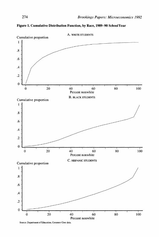
If schools were perfectly integrated, so that every school's enrollment was in proportion to the share of each racial group in the population, there would be little concern over the allocation of resources in schools along racial lines. This is not the case. We have used the Department of Education's annual survey of schools, known as Common Core, to examine the extent of racial segregation in public schools.8 A high degree of segregation exists in public schools. According to our esti- mates, in school year 1989-90, for example, the average black student attended a school in which 65 percent of the students were nonwhite, while the average white student attended a school in which 17 percent of the students were nonwhite. The average Hispanic student attended a school in which 68 percent of the students were either black or Hispanic.
Figure 1 shows the cumulative proportions of black, white, and Hispanic students who attend a school with less than the specified proportion of minority students.9 Notice the sharp increase in these cumulative distribution functions around 95 percent for black and His- panic students. By contrast, there is a sharp increase between 0 and 5 percent for white students. Roughly 30 percent of black students attend schools whose enrollment is more than 95 percent nonwhite, while more than 30 percent of white students attend schools that have less than 5 percent nonwhite students. At all levels, the cumulative distributions are very similar for black and Hispanic students.
7. See Hanushek (1986) for a survey of school resources and test scores. See Card and Krueger (1992b) for evidence on school resources and labor market success.
8. This data set contains information on the racial composition of students in 81,368 schools in 43 states and the District of Columbia. Given this large sample size, our estimates are extremely precise, and we do not, therefore, present standard errors.
9. For the purposes of this paper, black refers to black, non-Hispanic origin, and white refers to white, non-Hispanic origin. The term minority refers to all groups other than white, non-Hispanics.
274 Brookings Papers: Microeconomics 1992
Figure 1. Cumulative Distribution Function, by Race, 1989-90 School Year
A. WHITE STUDENTS Cumulative proportion
.8--
.6-
.4-
.2-
0 0 - I l l l l l
0 20 40 60 80 100 Percent nonwhite
B. BLACK STUDENTS Cumulative proportion
.8-
.6 -
.4 -
.2
0 ~I I I - I ' ' -'
0 20 40 60 80 100 Percent nonwhite
C. HISPANIC STUDENTS Cumulative proportion
.8
.6-
.4-
.2
0 O - l I . I
0 20 40 60 80 100 Percent nonwhite
Source: Department of Education, Common Core data.

Michael A. Boozer, Alan B. Krueger, and Shari Wolkon 275
The extent of segregation is far greater in public schools in large center cities (those with a population of at least 400,000). Figure 2 presents graphs of the cumulative percentages of white and black stu- dents who attend schools with less than the specified percentages of nonwhite students, broken down by whether or not the school is in a large center city. Nearly two-thirds (64 percent) of black students in public schools in large center cities attend schools in which at least 90 percent of the enrolled students are nonwhite, whereas less than 15 percent of black students outside of large cities attend schools that are at least 90 percent nonwhite.10 In contrast, only 3 percent of white students in large center cities attend a school with 90 to 100 percent minority enrollment. Furthermore, 34 percent of black students live in large center cities, compared with 6 percent of white students. We are unaware of comparable data to assess whether or how these percentages have changed over time. Welch and Light, however, found that the percentage of white students attending selected central city school dis- tricts had declined sharply in every region of the country between 1968 and 1980.11
The most widely cited historical evidence on the extent of public school desegregation in the United States is based on the work of Gary Orfield, who analyzed school-level data on students' race supplied by the U.S. Department of Education.12 These data cover only 1968 through 1980.13 Furthermore, 1968 is considered a benchmark year in the prog- ress of school desegregation because in that year the Supreme Court held in Green v. County Board of Education of New Kent County that "freedom of choice" was no longer a viable means of desegregating noncompliant school districts.14 Unfortunately, little is known about the efficacy of school desegregation before 1968, so it is not clear whether Green instigated a change in racial segregation. Here we pro- vide some new evidence on segregation trends in the years around 1968
10. The level of segregation is even greater in large center cities in certain regions. In the Northeast 70 percent of black students are enrolled in schools that have at least 90 percent minority enrollment. The comparable figure for the border states is 77 percent.
11. Welch and Light (1987). 12. Orfield (1983). 13. Earlier work by Coleman, Kelly, and Moore (1975) uses data from 1968 to 1973
to analyze the extent of racial segregation at the school district level. These data suffer from missing any segregation within individual districts.
14. Hochschild (1984, p. 27).

276 Brookings Papers: Microeconomics 1992
Figure 2. Cumulative Distribution by Location of School and Race, 1989-90 School Year
A. WHITE STUDENTS
Cumulative proportion
.9
.8
.7
.6
.4- ,/ Center city
, Outside center city
.1
0
0 10 20 30 40 50 60 70 80 90 100 Percent nonwhite
B. BLACK STUDENTS
Cumulative proportion
.9
.8 Center city Outside center city
.7
.6
.5
.4
.3
.2
.1
0 -
0 10 20 30 40 50 60 70 80 90 100 Percent nonwhite
Source: Department of Education, Common Core data.

Michael A. Boozer, Alan B. Krueger, and Shari Wolkon 277
Table 1. Attendance of Black Students at Minority Schools, Selected Years, 1968- 89
Region 1968 1972 1976 1980 1989
Percentage of black students in predominantly minority schools Southa 80.9 55.3 54.9 57.1 59.5 Borderb 71.6 67.2 60.1 59.2 58.5 Northeastc 66.8 69.9 72.5 79.9 75.4 Midwestd 77.3 75.3 70.3 69.5 69.7 Weste 72.2 68.1 67.4 66.8 68.5
U.S. 76.6 63.6 62.4 62.9 65.1
Percentage of black students in 90-100% minority schools South 77.8 24.7 22.4 23.0 26.0 Border 60.2 54.7 42.5 37.0 33.6 Northeast 42.7 46.9 51.4 48.7 49.9 Midwest 58.0 57.4 51.1 43.6 40.1 West 50.8 42.7 36.3 33.7 27.1
U.S. 64.3 38.7 35.9 33.2 33.8 Sources: Data for 1968-80 are from Orfield (1983, p. 4) and are based on U.S. Department of Education data; data for 1989
are authors' calculations based on the Common Core Public School Universe File, Department of Education. Data for Alaska and Hawaii are not included. Data are unavailable for Georgia, Idaho, Maine, Missouri, South Dakota, Virginia, and Wyoming. Predominantly minority means that more than half of the students in the school are nonwhite.
a. Alabama, Arkansas, Florida, Georgia, Louisiana, Mississippi, North Carolina, South Carolina, Tennessee, Texas, and Virginia.
b. Delaware, District of Columbia, Kentucky, Maryland, Missouri, Oklahoma, and West Virginia. c. Connecticut, Maine, Massachusetts, New Hampshire, New Jersey, New York, Pennsylvania, Rhode Island, and Vermont. d. Illinois, Indiana, Iowa, Kansas, Michigan, Minnesota, Nebraska, North Dakota, Ohio, South Dakota, and Wisconsin. e. Arizona, California, Colorado, Idaho, Montana, Nevada, New Mexico, Oregon, Utah, Washington, and Wyoming.
and also update Orfield's original estimates of racial segregation through 1989.
The Common Core data for school year 1989-90 are used to update Orfield's estimates of the percentage of black students enrolled in pre- dominantly minority schools (those with minority enrollment of 50 percent or more) and in schools with at least 90 percent minority en- rollment.15 Table 1 presents Orfield's estimates of the extent of seg- regation for 1968-80, and our estimate for 1989.16 It is clear from the
15. Orfield (1983, p. 4). Although many other indices of school segregation are possible, we use these measures for historical comparison.
16. Although we lack data for seven states, if we recompute Orfield's estimates for 1980 using just the subset of states included in our data set, none of our conclusions is meaningfully altered. For example, using our subset, in 1980 the estimate of the percent of black students in at least 90 percent minority schools in the South is 24.6 percent, which is close to Orfield's original estimate of 23.0 percent. The estimates for the other regions are even closer. For this reason, we do not adjust Orfield's estimates.
278 Brookings Papers: Microeconomics 1992
table that the degree of segregation in the nation as a whole dropped precipitously between 1968 and 1972 and then remained roughly con- stant over the 1970s. Our extension of these data through the 1989-90 school year reveals that racial isolation for black students increased slightly in the 1980s.
The trends in school desegregation differ across regions of the coun- try. The decline in segregation between 1968 and 1972 was concentrated primarily in the southern and border states. In 1968, 77.8 percent of black students in the South attended schools where minority students constituted at least 90 percent of the student body; this figure dropped to 24.7 percent just four years later. School segregation appears to have increased in the South since the mid-1970s. Observing the high rate of segregation in Orfield's data for the South in 1968, some scholars have concluded that desegregation did not occur on a wide scale before 1968.
Between 1968 and 1989, school segregation for black children grad- ually declined in the border states, the Midwest, and the West. In the Northeast, however, black students are now substantially more racially isolated than they were in 1968. While school segregation rapidly de- clined in the South between 1968 and 1972, the Northeast experienced a rise in school segregation. Moreover, despite the upward drift in school segregation in the South, that region now has the highest level of racial integration in schools, and the Northeast is now the region of the country where minority students are most racially isolated.
HISPANIC STUDENTS. The pattern of segregation for Hispanic students is presented in table 2. Unlike black students, Hispanic students did not experience a dramatic decline in segregation between 1968 and 1972. Moreover, in almost every region and every time period for which we have data, Hispanic students have become increasingly more racially isolated. 17 The greatest increase in the number of Hispanic students has occurred in the West and Midwest, and these regions have experienced the greatest increases in segregation. As a consequence, Hispanic stu- dents now face roughly the same level of racial isolation in schools as black students do. To the extent that language is also a barrier for
17. The extent of segregation for Hispanic students is also greater in urban areas. In cities with 400,000 or more people, 55 percent of Hispanic students are enrolled in schools with at least 90 percent minority enrollment.

Michael A. Boozer, Alan B. Krueger, and Shari Wolkon 279
Table 2. Attendance of Hispanic Students at Minority Schools, 1968-89
Area 1968 1972 1976 1980 1989
Percentage of Hispanic students in predominantly minority schools South 69.6 69.9 70.9 76.0 76.1 Border ... ... ... ... Northeast 74.8 74.4 74.9 76.3 75.9 Midwest 31.8 34.4 39.3 46.6 53.1 West 42.4 44.7 52.7 63.5 71.6
U.S. 54.8 56.6 60.8 68.1 72.0
Percentage of Hispanic students in 90-100% minority schools South 33.7 31.4 32.2 37.3 38.5 Border ... ... . Northeast 44.0 44.1 45.8 45.8 43.0 Midwest 6.8 9.5 14.1 19.6 22.1 West 11.7 11.5 13.3 18.5 27.9
U.S. 23.1 23.3 24.8 28.8 32.7 Sources: Data for 1968-80 are from Orfield (1983, p. 14) and are based on U.S. Department of Education data; data for
1989 are authors' calculations based on the Common Core Public School Universe File, Department of Education. Data for Alaska and Hawaii are not included. Data are unavailable for Georgia, Idaho, Maine, Missouri, South Dakota, Virginia, and Wyoming. Results are not reported for border states because the number of Hispanic students is small. Predominantly minority means that more than half of the students in the school are nonwhite. See table I for definitions of regions.
Hispanic students, this trend toward increasing segregation may have great consequences.18
NEW HISTORICAL EVIDENCE. Attempts to interpret historical trends in school desegregation have been hamstrung by the lack of comparable data before the Green decision in 1968. In particular, the Civil Rights Act of 1964 may have reduced the extent of school segregation by prohibiting federal aid to segregated institutions. The incentive for dis- tricts to desegregate was further strengthened by the passage of the Elementary and Secondary Education Act of 1965, which gave addi- tional federal aid to desegregated school districts. In short, beginning in 1964 the federal government provided financial incentives for school districts to desegregate, and the Civil Rights Act enabled the Justice Department to join in suits against noncompliant school districts.19
To measure the extent to which the move toward desegregation was
18. Hochschild (1984, p. 45). 19. Hochschild (1984, p. 27).

280 Brookings Papers: Microeconomics 1992
already under way in the southern and border states before 1968, we analyze data from the National Survey of Black Americans (NSBA).20 In 1980 the NSBA asked black Americans aged 18 or older whether they had attended an "all black" or "mostly black" grammar, junior high, or high school. The survey also identified the state the individuals grew up in and their age. We used this information to construct a time series of data on school segregation. Specifically, we inferred the cal- endar year in which each individual would have been in elementary, junior high, or high school, and then pooled the data to derive an estimate of the extent of segregation each year.21 This procedure is likely to smooth the actual series, making it difficult to determine pre- cisely the year of breaks in the series.22 We are able, however, to examine the extent of school segregation with comparable data over a broad sweep of history (1924-71).
The results of this exercise are summarized in figure 3, and the underlying data are reported in appendix table A-1. For each calendar year, the figure presents an estimate of the proportion of students who attended an all black school (figure 3A) or a majority black school (figure 3B) and places a one standard error bound around the estimate. Our estimates are in broad agreement with Orfield's in the years in which the two studies overlap (1968-7 1). These figures also make clear that before the Brown decision, virtually all black students attended completely segregated schools in the southern and border states. Our estimates document that segregation did not decline in the 10 years following the Brown decision.
Surprisingly, the figures indicate that 1964, not 1968, was a wa- tershed year in the history of school desegregation in the southern and
20. The data for the National Survey of Black Americans 1979-80, were originally collected by James S. Jackson and Gerald Gurin. We limit the sample to individuals who grew up in the southern and border states. The survey was published in 1987 in Ann Arbor, Mich., by the Inter-university Consortium for Political and Social Research.
21. Specifically, we assumed that individuals' response to the grammar school question corresponded to the year in which they turned 9, their response to the junior high question corresponded to the year in which they turned 14, and their response to the high school question corresponded to the year they turned 16.
22. Our results, however, are almost numerically equivalent when we limit the sample to the high school and junior high questions, which cover a much narrower time span than grade school does. This finding suggests that smoothing may not be a serious problem. We retain the grammar school data in the graphs presented to increase the sample size. The total sample size used to create figure 3 is 4,152.

Michael A. Boozer, Alan B. Krueger, and Shari Wolkon 281
Figure 3. Segregation in Southern and Border States, 1924-71
A. Proportion of blacks attending all black schools a
Percent
1002 80-
70 -
60-
50-
40-
30-
20-
10 l
1924 1934 1944 1954 1964 1968 1971
B. Proportion of blacks attending majority black schoolSc Percent
80-
70-
60-
50-
40-
30-
20-
10
1924 1934 1944 1954 1964 1968 1971 Source: Authors' calculations based on data from the National Survey of Black Americans. a.Dashed lines are plus and minus 1 standard error.
282 Brookings Papers: Microeconomics 1992
border states. Despite the smoothing due to the use of retrospective data, the trend toward school integration clearly began before 1968. These results suggest that, contrary to widespread belief, federal leg- islation that took effect before 1968 was a catalyst for the reduction in school segregation in the South.
Pupil-Teacher Ratio
Throughout the first half of the twentieth century, the typical black student attended a school with far more students per class than did the typical white student. There are two principal reasons for this disparity. First, a disproportionately large number of black students lived in the South, and the quality of schools in the South lagged well behind the rest of the nation at the beginning of the century. Second, within the South black students were confined to racially segregated schools that were understaffed and overcrowded relative to schools attended by white students. In the twentieth century, however, the pupil-teacher ratios for white and black students have tended toward equality because the gap in class size for black and white students within regions has narrowed substantially, the South has caught up with the rest of the nation in terms of school resources, and the share of blacks living in the South has declined.23
Figures 4 and 5 present graphs of the relative white-black pupil- teacher ratio and of the gap in the pupil-teacher ratio between black schools and white schools between 1915 and 1989 for the 17 states and the District of Columbia that had legally segregated schools before the Brown decision.24 In 1915 the average pupil-teacher ratio in black schools in these states was 60.8, far greater than the average of 37.6 in white schools. In 1953-54, on the eve of the Brown ruling, the pupil-teacher ratio was 31.6 for black students and 27.6 for white students. Although government records are limited after this period, data from the Southern
23. Note that the terms class size and pupil-teacher ratio are used interchangeably. 24. These figures are based on data from the Biennial Surveys of Education published
by the Department of the Interior, Bureau of Education, state education reports, and the authors' calculations using the Common Core data set. The pre-1966 data are described in more detail in Card and Krueger (1992a). The term length and average teacher salary show similar trends through 1966. Also see Smith and Welch (1989, table 17) for related evidence. Henceforth, we refer to the District of Columbia as a state. Comparable data do not exist for states outside the South.

Michael A. Boozer, Alan B. Krueger, and Shari Wolkon 283
Figure 4. Relative White-Black Pupil-Teacher Ratio White/black pupil-teacher ratio
0.9 -
0.8-
0.7 -
1915 1925 1935 1945 1955 1965 1975 1989 Source: Authors' calculations based on data from the Department of Interior. Biennzial Survevs of Education, and the
Department of Education Common Core data set. The vertical line highlights 1954.
Educational Reporting Service indicate that in 1966 the average pupil- teacher ratio was 26.1 for black students and 24.0 for white students. Notice that there is no apparent break in the series around 1954; if anything, relative progress for black students was slower in the decade following Brown than in the decade preceding the decision.25
Little is known about the pupil-teacher ratio for the average black student and average white student since 1966. Until recently the De- partment of Education did not include the number of students enrolled in a school by race in the public-use extract of its basic data set, Common Core. The 1987-90 Common Core public-use data sets specify the number of students in a school, the race of the students, and the number of teachers in the school for every public elementary and secondary school in 40 states. We have used these data to calculate the pupil-
25. Some states even show a decline in relative school quality just after the Brown decision. These observations reinforce Donohue and Heckman's (1990) contention that there was not a discrete improvement in school quality for black students around 1954.

284 Brookings Papers: Microeconomics 1992
Figure 5. White-Black Gap in Pupil-Teacher Ratio
White-black pupil-teacher gap 0
-5
-10
-15
-20
-25
1915 1925 1935 1945 1955 1965 1975 1989 Source: See figure 4.
teacher ratio for an average member of each race by the following weighted average:
PTr = I PT, NM / (E N%),
where PTr is the average pupil-teacher ratio for a member of race r, PTi is the ratio of pupils to teachers in school i, and Nr is the number of students in school i who belong to race r.26 The summation runs over all schools. This procedure is equivalent to assigning to all students in the school the pupil-teacher ratio for that school and then calculating the mean pupil-teacher ratio for members of each race separately.
This approach has some obvious shortcomings. First, using school- level data misses any possible differences in class size by race within schools. Second, in 1980, 11.4 percent of white students and 5.4 percent of black students attended private and parochial schools.27 The Common Core files do not have data on the racial composition of students at-
26. This is the same approach used in Coleman and others (1979). 27. These figures are based on Welch and Light (1987, table 3).

Michael A. Boozer, Alan B. Krueger, and Shari Wolkon 285
Table 3. Pupil-Teacher Ratio for Black, Hispanic, and White Students in 1989
Average ratio Percent ratio > 25
Area Black Hispanic White Black Hispanic White
All grade levels South 17.8 17.9 17.9 1.4 2.7 1.8 Border 18.4 17.6 17.7 1.5 1.1 1.0 Northeast 16.4 16.2 15.8 1.1 0.8 1.0 Midwest 18.1 18.5 17.7 2.6 5.6 2.7 West 22.9 23.2 22.3 29.4 32.6 23.4
U.S. 18.1 20.3 18.3 4.2 17.1 6.2
Grammar school South 18.3 18.1 18.5 1.8 2.2 2.0 Border 19.6 18.7 18.6 1.7 1.6 1.7 Northeast 17.8 17.5 17.6 1.9 1.0 1.7 Midwest 18.9 18.9 18.9 3.7 5.0 4.3 West 23.9 24.1 23.4 38.1 43.0 23.4
U.S. 19.0 21.1 19.6 5.9 22.6 9.5
High school South 17.0 17.7 17.0 0.7 3.6 0.9 Border 16.9 16.0 16.8 0.3 0.0 0.2 Northeast 15.6 15.3 13.9 0.0 0.0 0.1 Midwest 16.8 16.9 16.3 0.2 0.4 0.5 West 22.0 22.5 21.2 20.5 23.7 12.7
U.S. 17.2 19.7 17.0 2.2 12.7 2.7 Source: Tabulated by authors from the Common Core Public School Universe File, Department of Education. Data for Alaska
and Hawaii are not included. Data are unavailable for Georgia, Idaho, Maine, Massachusetts, Missouri, Montana, Rhode Island, South Dakota, Virginia, and Wyoming. See table I for definitions of regions.
tending private schools, so any difference in class size between public schools and private schools is not reflected in these estimates.28 Third, 11 states in the Common Core survey do not report complete data on students' race or on the number of teachers, and these states are therefore omitted from the estimates. Nevertheless, our weighted averages of pupil-teacher ratios at the school level provide at least a partial picture of the quantity of school resources available to students of different races.
Table 3 reports estimates of the average pupil-teacher ratio for black,
28. Estimates presented later for high school students based on the High School and Beyond Survey do include private schools, however.

286 Brookings Papers: Microeconomics 1992
Hispanic, and white students during school year 1989-90. The table also reports the proportion of students of each race who attend schools that have more than 25 students per teacher. (Appendix table A-2 reports estimates by state.) The estimates are based on a total sample of 69,610 schools.
Perhaps surprisingly, table 3 indicates that the pupil-teacher ratio is slightly higher for white students (18.3) than for black students (18.1). The long period of a higher pupil-teacher ratio for black students has finally come to an end. In contrast, the pupil-teacher ratio of the average Hispanic student (20.3) is 11 percent higher than that of the average white student.
Inspection of table 3 reveals some interesting regional patterns. First, the pupil-teacher ratio is significantly higher in the West than in the rest of the country. Hispanic students are vastly overrepresented in the West, which helps explain the relatively high pupil-teacher ratio for these students. Second, black students currently have a higher pupil- teacher ratio than do white students in all regions of the country but the South. In the Northeast, for instance, there is an average of 0.6 more students per teacher in the average school attended by black stu- dents than there is in the average school attended by white students, and the difference is 1.7 students per teacher for high schools.
Hispanic students at higher grade levels are also at a greater relative disadvantage as far as class size is concerned. The average pupil-teacher ratio for Hispanic high school students exceeds the average for white high school students by 16 percent. Moreover, the high school dropout rate for Hispanic students is 35.8 percent, far higher than the dropout rate of 12.7 percent for white students and 14.9 percent for black students.29 Any decline in the dropout rate for Hispanic students is likely to increase the gap in the pupil-teacher ratio between Hispanic students and other students. Conversely, the relatively high pupil-teacher ratio for Hispanic high school students may contribute to their higher dropout rate.
WITHIN-STATE PATTERNS. Several scholars, including W. E. B. Du- bois and Horace Mann Bond, have noted that across regions of the
29. These figures are "status" dropout rates, and pertain to 16-24-year-olds. The data are based on the Bureau of the Census, Current Population Survey, October 1988, and are reported in Schick and Schick (1991).

Michael A. Boozer, Alan B. Krueger, and Shari Wolkon 287
country, expenditures per student in black schools relative to white schools are inversely related to the fraction of blacks in the population. This pattern was carefully documented with county-level data by Bond in 1934 and by Margo in 1990.30 Bond summarizes:
Negro schools are financed from the fragments which fall from the budget made up for white children. Where there are many Negro children, the available funds are given principally to the small white minority. Besides depressing expenditures for Negro children, expenditures for white chil- dren in these heavily populated Negro counties are far above the median for the entire state.31
Bond argued that this pattern developed because state funds were al- located on a per-student basis, which enabled school superintendents to divert more funds to white schools in areas that were heavily pop- ulated by blacks. Because black voters were effectively disenfranchised, they did not have the means to stop this process.
Figure 6 uses data for the southern and border states for each decade since 1920 to illustrate that the relationship documented by Bond across counties also exists at the state level.32 Until 1960 the plots show a strong, persistent negative relationship between the percentage of the population in a state that is black and the ratio of the pupil-teacher ratio in white schools to that in black schools. That relationship has weakened with time and is totally eliminated by school year 1989-90. In fact, a weak positive relationship is found if all states (not just the southern and border states) are used. This turnaround is likely a result of increased voting rights for black citizens over the years.
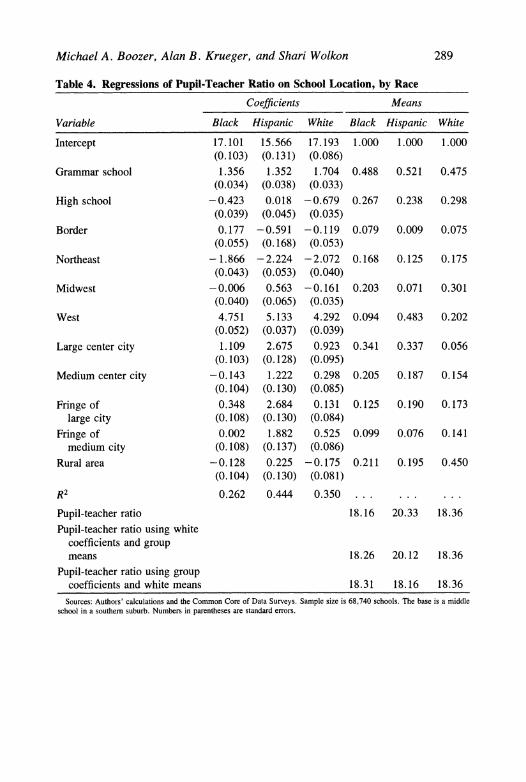
SCHOOL-LEVEL ANALYSIS. We have used the Common Core data to estimate some descriptive regressions of the relationship among the pupil-teacher ratio, school location, and race. These regressions are summarized in table 4. The first three columns report estimates weighted by the number of black, Hispanic, and white students in the school. The last three columns present the weighted means of the variables.
The regressions reveal several patterns. First, schools located in the
30. Bond (1934); and Margo (1990). 31. Bond (1934, pp. 244-45). 32. Our data on the fraction of the population that is black is from decennial censuses
of the population, as reported in various issues of Statistical Abstract of the United States, published by the Bureau of the Census. The figure for 1990 uses data for 15 states.

288 Brookings Papers: Microecon(omics 1992
Figure 6. Relative School Quality v. Percent of Population That Is Black
A. 1920 B. 1930 White-black pupil-teacher ratio White-black pupil-teacher ratio
1.1- * 1.1-
1.0 * 1.0 0.9 * 0.9 0.8 - 0.8 0.7 * 0.7 0.6 - 0.6 0.5- 0.5 0.4 0.4 _ ,_,_-_,_-_----- _r
0 10 20 30 40 50 0 10 20 30 40 50 Percent black Percent black
C. 1940 D. 1950 White-black pupil-teacher ratio White-black pupil-teacher ratio
1.1 . 1.1 1.0 1.0 0.9 . 0.9 **
0.8 0.8 0.7 0.7 0.6 0.6 0.5 0.5 0.4 _ _ _ _ _ _ _ _ ;_ ,_ 0.4
0 10 20 30 40 50 0 10 20 30 40 50 Percent black Percent black
E. 1960 F. 1990 White-black pupil-teacher ratio White-black pupil-teacher ratio
1.1 * 1.1
1.0 * 1.0
0.9 0.9 0.8 0.8 0.7 * 0.7 0.6 0.6 0.5 0.5 0.4 - _,_. _, _- _, _ 0.4 A-
0 10 20 30 40 50 0 10 20 30 40 50 Percent black Percent black
Source: Authors' calculations based on various issues of Staitistical Abstract. Bureau of the Census.
Michael A. Boozer, Alan B. Krueger, and Shari Wolkon 289
Table 4. Regressions of Pupil-Teacher Ratio on School Location, by Race
Coefficients Means
Variable Black Hispanic White Black Hispanic White
Intercept 17.101 15.566 17.193 1.000 1.000 1.000 (0.103) (0.131) (0.086)
Grammar school 1.356 1.352 1.704 0.488 0.521 0.475 (0.034) (0.038) (0.033)
High school -0.423 0.018 -0.679 0.267 0.238 0.298 (0.039) (0.045) (0.035)
Border 0.177 -0.591 -0.119 0.079 0.009 0.075 (0.055) (0.168) (0.053)
Northeast -1.866 -2.224 -2.072 0.168 0.125 0.175 (0.043) (0.053) (0.040)
Midwest -0.006 0.563 -0.161 0.203 0.071 0.301 (0.040) (0.065) (0.035)
West 4.751 5.133 4.292 0.094 0.483 0.202 (0.052) (0.037) (0.039)
Large center city 1.109 2.675 0.923 0.341 0.337 0.056 (0.103) (0.128) (0.095)
Medium center city -0.143 1.222 0.298 0.205 0.187 0.154 (0.104) (0.130) (0.085)
Fringe of 0.348 2.684 0.131 0.125 0.190 0.173 large city (0.108) (0.130) (0.084)
Fringe of 0.002 1.882 0.525 0.099 0.076 0.141 medium city (0.108) (0.137) (0.086)
Rural area -0.128 0.225 -0.175 0.211 0.195 0.450 (0.104) (0.130) (0.081)
R 2 0.262 0.444 0.350 ... ... ...
Pupil-teacher ratio 18.16 20.33 18.36 Pupil-teacher ratio using white
coefficients and group means 18.26 20.12 18.36
Pupil-teacher ratio using group coefficients and white means 18.31 18.16 18.36
Sources: Authors' calculations and the Common Core of Data Surveys. Sample size is 68,740 schools. The base is a middle school in a southern suburb. Numbers in parentheses are standard errors.
290 Brookings Papers: Microeconomics 1992
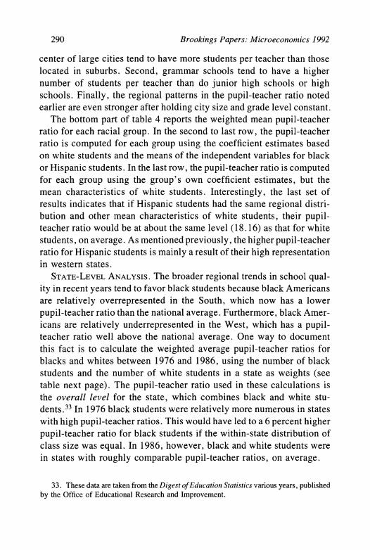
center of large cities tend to have more students per teacher than those located in suburbs. Second, grammar schools tend to have a higher number of students per teacher than do junior high schools or high schools. Finally, the regional patterns in the pupil-teacher ratio noted earlier are even stronger after holding city size and grade level constant.
The bottom part of table 4 reports the weighted mean pupil-teacher ratio for each racial group. In the second to last row, the pupil-teacher ratio is computed for each group using the coefficient estimates based on white students and the means of the independent variables for black or Hispanic students. In the last row, the pupil-teacher ratio is computed for each group using the group's own coefficient estimates, but the mean characteristics of white students. Interestingly, the last set of results indicates that if Hispanic students had the same regional distri- bution and other mean characteristics of white students, their pupil- teacher ratio would be at about the same level (18. 16) as that for white students, on average. As mentioned previously, the higher pupil-teacher ratio for Hispanic students is mainly a result of their high representation in western states.
STATE-LEVEL ANALYSIS. The broader regional trends in school qual- ity in recent years tend to favor black students because black Americans are relatively overrepresented in the South, which now has a lower pupil-teacher ratio than the national average. Furthermore, black Amer- icans are relatively underrepresented in the West, which has a pupil- teacher ratio well above the national average. One way to document this fact is to calculate the weighted average pupil-teacher ratios for blacks and whites between 1976 and 1986, using the number of black students and the number of white students in a state as weights (see table next page). The pupil-teacher ratio used in these calculations is the overall level for the state, which combines black and white stu- dents.33 In 1976 black students were relatively more numerous in states with high pupil-teacher ratios. This would have led to a 6 percent higher pupil-teacher ratio for black students if the within-state distribution of class size was equal. In 1986, however, black and white students were in states with roughly comparable pupil-teacher ratios, on average.
33. These data are taken from the Digest of Education Statistics various years, published by the Office of Educational Research and Improvement.

Michael A. Boozer, Alan B. Krueger, and Shari Wolkon 291
Current weights 1976 weights Year White Black White Black 1976 21.87 23.18 21.87 23.18 1980 18.88 19.02 18.84 18.99 1984 18.23 18.32 18.18 18.27 1986 17.82 17.97 17.73 17.75
Is the convergence in pupil-teacher ratio (at the state level) between blacks and whites attributable to migration of black students from states with large class sizes to states with small class sizes, or does it come from a relative improvement in class size in states where black students are overrepresented? To answer this question, the distribution of stu- dents across states was held constant at its 1976 level, and the weighted averages were recomputed. The last two columns show quite clearly that this convergence occurred because average class size declined in states where black students were relatively more numerous.
WEALTH AND THE PUPIL-TEACHER RATIO. Although race does not seem to be a major factor in determining class size, evidence suggests that schools in districts with lower property values tend to have larger pupil-teacher ratios. For example, figure 7 presents a scatter diagram of the ratio of pupils to teachers in 274 school districts in Massachusetts in 1990 against the log of the equalized property value for the districts in 1988.34 Notice the wide variation in the pupil-teacher ratio across districts-the top percentile of school districts has an average of 10 students per teacher, while the bottom percentile of districts has an average of 22 students per teacher. The figure also shows a strong inverse relationship between the pupil-teacher ratio and property value. The OLS regression of the pupil-teacher ratio on the log of equalized property value is
Pupil-teacher ratio 35.17 - 3.56 ln(land value). (2.56) (0.47)
R2=0.17.
The relationship between the pupil-teacher ratio and land value is highly
34. The property value data are from unpublished tables prepared by the Massachusetts Department of Education.

292 Brookings Papers: Microeconomics 1992
Figure 7. Pupil-Teacher Ratio v. Land Value, Massachusetts
Pupil-teacher ratio 0
25 -
0
O ooO
0 0 0 0 SO~Oc ~ 0
0 - l l 0 0
15 0 6~ 6.500 0
0~~~~ ~L lan vau per CC)den
staistcalyignficnt(t-rti = 7.7) A 20 pecn inraenln
0 0 ~0 00 0 ~~' 00 0
h0 alo 0 0
00 0 ~ 0 0( 0 0~~~~~~~ 0~~~~~~ 0 ~~0 0
5 5.5 6 6.5 7 Ln land value per student
Source: Massachusetts Department of Education, unpublished data.
statistically significant (t-ratio =7.57). A 20 percent increase in land value is associated with about 0.7 fewer students per teacher.
We have also analyzed the relationship between the median salary of teachers in a school district in Massachusetts and the log of equalized property value. The estimated regression equation is given below:
Median salary 7227.9 + 5130.4 ln(land value) (4956.1) (917.1)
R2 = 0. 1 1.
There is a highly statistically significant relationship (t-ratio = 5.59) between median teacher salary and the property wealth of a school district. A 20 percent increase in property value, for example, is as- sociated with more than $1,000 in higher annual pay for the median teacher.
We prefer not to put a structural interpretation on either of these estimated relationships because the direction of causality is not clear. Higher quality schools may increase the land values in a school district,

Michael A. Boozer, Alan B. Krueger, and Shari Wolkon 293
but it is also plausible that higher income individuals choose to provide their children with higher quality schools. Nevertheless, these results indicate that more school resources are available to children who grow up in wealthier areas. It is therefore noteworthy that the estimates in table 3 do not show much of a gap in class size between white and black students, even though black families are more likely than white families to live in low-income areas.35
Perhaps schools attended by minority students have been able to maintain roughly comparable levels of class size as schools attended by white students by forgoing other resources that are provided to students in wealthier areas. Next we present evidence suggesting that race does have an effect on a more modern measure of school quality, namely, the extent of computer use by students.
Computer Utilization
The computer revolution of the 1980s has had a profound effect on the operation and organization of elementary and secondary schools. The number of computers in use in elementary and secondary schools increased by more than 1,700 percent between 1981 and 1988. In 1988, 1.52 million microcomputers were used for instructional purposes in public schools-one computer for every 26.9 students.36 Computer labs are common in public and private schools, and many private schools compete for students by advertising their computer resources. In 1989 nearly half of all students reported that they directly use computers in school. Schools use computers for two purposes: to aid instruction, and to provide students with computer skills that are of use in the labor market and elsewhere.
To date, only two studies have been conducted to determine the extent of students' computer use by race.37 Both of these studies ana- lyzed data from the early 1980s, before the widespread adoption of
35. For example, Blau and Graham (1989) estimate that in the late 1970s, the average black married couple had about one-third as much equity in housing as the average white married couple ($4,222 versus $13,864). For this sample blacks had three-fourths the income of whites. Based on the relationship for Massachusetts, a property wealth differential of 66 percent would be expected to increase the pupil-teacher ratio by about 2.3 pupils.
36. Private schools had one computer for every 23.5 students. These figures are drawn from Statistical Abstract of the United States, 1990, tables 238 and 1340.
37. McPhail (1985).

294 Brookings Papers: Microeconomics 1992
Table 5. Students Who Use Computers in School, by Race Percent
Grade 1984 1989
All grades White 36.3 56.4 Black 18.3 39.3 Hispanic 19.9 41.9
Grades 1-8 White 38.5 60.9 Black 16.8 38.4 Hispanic 19.4 42.7
Grades 9-12 White 31.8 45.5 Black 21.6 41.5 Hispanic 21.3 39.6
Source: Authors' tabulations based on the October Cuirrenzt Populationz Sunrey, 1984 and 1989. Total sample size is 23,295 in 1989 and 25,067 in 1984. White is defined as white, non-Hispanic; black is defined as black, non-Hispanic.
computers in schools. To explore racial differences in computer use in schools more recently, we analyzed data from the 1984 and 1989 October Current Population Survey (CPS) School Enrollment Supple- ment microdata files. In these two supplements, respondents were asked: "Does . . . directly use a computer at school?"38 In addition to being more recent than the data analyzed by the previous researchers, these data files provide large, nationally representative samples with detailed demographic information on students and their families. Our sample was limited to students aged 6 to 18 who were enrolled in grades 1 through 12.
Table 5 reports our estimates of the proportion of students who used computers in school by grade level and race in 1984 and 1989. Between 1984 and 1989, this proportion grew substantially. Black students, however, were much less likely to use a computer in school than white students. Across all grade levels in 1984, 36 percent of white pupils but only 18 percent of black pupils used computers in school. And computer utilization was not much greater among Hispanic students than among black students.
38. According to the questionnaire, computer use means: " 'Direct' or 'hands on use' of computers. These computers may be personal computers, minicomputers, or mainframe computers." Excluded are "hand-held calculators or games, electronic video games, or systems which do not use a typewriter-like keyboard."
Michael A. Boozer, Alan B. Krueger, and Shari Wolkon 295
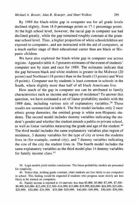
By 1989 the black-white gap in computer use for all grade levels declined slightly, from 18.0 percentage points to 17.1 percentage points. At the high school level, however, the racial gap in computer use had declined greatly, while the gap remained roughly constant at the gram- mar school level. Thus, a higher proportion of white schoolchildren are exposed to computers, and are instructed with the aid of computers, at a much earlier stage of their educational career than are black or His- panic children.
We have also explored the black-white gap in computer use across regions. Appendix table A-3 presents estimates of the extent of students' computer use by state and race for 1989. The estimates indicate that the gap between black and white students is greater in the Midwest (20 points) and Northeast (18 points) than in the South (13 points) and West (9 points). Computer use by students is least common in schools in the South, where slightly more than half of all black Americans live.
How much of the gap in computer use can be attributed to family characteristics such as income and region of residence? To answer this question, we have estimated a set of linear probability models with the 1989 data, including various sets of explanatory variables.39 These results are summarized in table 6. The first model includes only 2 race/ ethnic group dummies; the omitted group is white non-Hispanic stu- dents. The second model includes dummy variables indicating the stu- dent's gender and whether the student attends a public or private school, as well as linear variables measuring the grade and age of the student.40 The third model includes the same explanatory variables plus region of residence, 3 dummy variables for the type of city or town the students lives in (for example, central city), and 7 dummy variables indicating the size of the city the student lives in. The fourth model includes the same explanatory variables as the third model plus 14 dummy variables for family income class.41
39. Logit models yield similar conclusions. The linear probability models are presented for simplicity.
40. Notice that, holding grade constant, older students are less likely to use computers in school. This finding would be expected if students who progress more slowly are less likely to be trained on computers.
41. Family income is reported in 14 intervals: less than $5,000, $5,000-$7,499, $7,500- $9,999,$10,000-$12,499,$12,500-$14,999,$15,000-$19,999,$20,000-$24,999,$25,000- $29,999, $30,000-$34,999, $35,000-$39,999, $40,000-$49,999, $50,000-$59,999,

296 Brookings Papers: Microeconomics 1992
Table 6. Determinants of Computer Use in Schools
Independent Linear probability model
variable 1 2 3 4
Intercept 0.564 0.749 0.768 0.663 (0.004) (0.030) (0.031) (0.034)
Black -0.171 -0.167 -0.122 -0.093 (1=yes) (0.009) (0.009) (0.010) (0.011)
Hispanic -0.144 -0.144 -0.105 -0.077 (1 = yes) (0.012) (0.012) (0.012) (0.013)
Female ... -0.010 -0.010 -0.009 (1=yes) (0.007) (0.006) (0.006)
Public school . .. -0.010 -0.017 -0.005 (1 = yes) (0.012) (0.012) (0.012)
Grade . .. 0.018 0.018 0.011 (0.005) (0.005) (0.005)
Age ... -0.026 -0.026 -0.020 (0.005) (0.005) (0.005)
Northeast ... ... 0.034 0.038 (1 = yes) (0.010) (0.010)
Midwest ... ... 0.018 0.024 (1 = yes) (0.010) (0.010)
South ... ... -0.053 -0.046 (1 = yes) (0.010) (0.010)
3 urban area type dummies included No No Yes Yes
7 SMSA size dummies included No No Yes Yes
14 income category dummies included No No No Yes
R 2 0.018 0.025 0.030 0.036 Source: Authors' calculations. Dependent variable equals I if student uses computer in school. Standard errors are shown in
parentheses. Sample size is 23,295. The data set used is the October 1989 Currenzt Population Survey.
Controlling for student characteristics, such as grade and age, does not reduce the magnitude of the racial gap in computer use. Including city size, city type, and region, however, reduces the black-white gap by about 5 percentage points, and the Hispanic-white gap by 4 points. Computer use at school is strongly related to family income. For ex- ample, children from families with $75,000 or more in annual income
$60,000-$74,999, $75,000 or more. We also include a dummy for family income not reported (5.8 percent of cases).

Michael A. Boozer, Alan B. Krueger, and Shari Wolkon 297
are 50 percent more likely to use computers in school than are children from families with less than $10,000 in annual income. Accounting for differences in family income reduces the gap in computer use relative to white students to 9.3 points for black students and 7.7 points for Hispanic students. In sum, accounting for all of these variables cuts the racial gap in school-related computer use roughly in half. Never- theless, the gap is still large and statistically significant.
For students aged 15 to 18, the CPS also contains information on whether the students' families have computers at home. In 1989, 35.8 percent of white students were in families that owned home computers, while only 15.3 percent of black students and 14.3 percent of Hispanic students had access to home computers. Furthermore, 29.7 percent of all white students but only 10 percent of black and Hispanic students used computers at home. In results not reported in the table, we find that students with computers available at home are 6.0 percentage points (t = 3.8) more likely to use a computer in school, after controlling for all the variables in model 4. Thus, less access to computers at home may further compound differences in computer use between minority and nonminority children.
A question of policy concern is: Why does the racial gap in computer use exist? There are four plausible explanations that should be inves- tigated. First, schools attended by minority students may lack sufficient resources to obtain computer equipment and still maintain adequate levels of other school resources, such as the student-teacher ratio. Sec- ond, teachers in schools attended by minority students may not know how to use computers effectively as teaching tools. Third, relatively large numbers of minority students may not come to school prepared to use computers. Fourth, computer distributors may have discriminated against inner-city schools in the provision of free computers or in com- puter prices.
Although all of these potential explanations cannot be addressed here, we can provide some information on the likely sources of the racial gap in computer use. First, however, we should stress that even if the average minority child comes to school less prepared to learn complex computer programming because of having a lower socioeconomic sta- tus, computers are widely used by schools for remedial education. Schools more frequently use computers as a learning device for a subject area than as a tool for teaching computer literacy. In this sense, com-
298 Brookings Papers: Microeconomics 1992
puter use is not like taking a course in an advanced subject. At the same time, if minority children are less likely to be exposed to com- puters at home, they may not see computers as a worthwhile tool to use in school.
Computer Use and Other Characteristics of High Schools: 1982
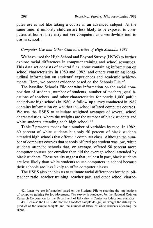
We have used the High School and Beyond Survey (HSBS) to further explore racial differences in computer training and school resources. This data set consists of several files, some containing information on school characteristics in 1980 and 1982, and others containing longi- tudinal information on students' experiences and academic achieve- ments. Here, we present evidence based on the Schools File.42
The baseline Schools File contains information on the racial com- position of students, number of students, number of teachers, qualifi- cations of teachers, and other characteristics for nearly 1,000 public and private high schools in 1980. A follow-up survey conducted in 1982 contains information on whether the school offered computer courses. We use the HSBS to calculate weighted averages of several school characteristics, where the weights are the number of black students and white students attending each high school.43
Table 7 presents means for a number of variables by race. In 1982, 60 percent of white students but only 50 percent of black students attended high schools that offered a computer class. Although the num- ber of computer courses that schools offered per student was low, white students attended schools that, on average, offered 50 percent more computer courses per enrollee than did the average school attended by black students. These results suggest that, at least in part, black students are less likely than white students to use computers in school because their schools are less likely to offer computer classes.
The HSBS also enables us to estimate racial differences for the pupil- teacher ratio, teacher training, teacher pay, and other school charac-
42. Later we use information based on the Students File to examine the implications of computer training for job placement. The survey is conducted by the National Opinion Research Corporation for the Department of Education's Center for Education Statistics.
43. Because the HSBS did not use a random sample design, we weight the data by the product of the sample weights and the number of black or white students attending the school.

Michael A. Boozer, Alan B. Krueger, and Shari Wolkon 299
Table 7. Mean High School Characteristics, by Race, 1980
Weighted by number of
Characteristic Black students White students
Proportion offering 0.50 0.60 computer courses (0.02) (0.02)
Number of computer 0.08 0.12 courses per 100 students (0.004) (0.007)
Pupil-teacher ratio 19.41 18.83 (0.14) (0.18)
Starting teacher $10,645 $10,485 salary (BA degree) (41) (42)
Proportion of teachers 0.52 0.47 with MA/Ph. D. (0.01) (0.01)
Percentage of teachers who 33.43 43.56 live within 5 miles (0.84) (0.91)
Percentage of teachers with 36.89 40.36 10 or more years experience (0.78) (0.78)
Percentage of teachers who 67.21 94.63 are white (0.89) (0.32)
Term length (days) 180.80 180.06 (0.18) (0.17)
Number of library 5,890 6,159 books (174) (162)
School has student 0.38 0.58 exchange program (0.02) (0.02)
School is under court 0.47 0.14 desegregation order (0.02) (0.01)
School is in urban area 0.49 0.14 (0.02) (0.01)
Number of security 2.28 0.66 guards (0.10) (0.05)
Source: Authors' calculations. The two questions on computers pertain to 1982. The sample consists of 975 high schools, containing 207,301 black students and 771,291 white students. Teacher salaries are in 1980 dollars. Data set: High School and Beyond Survey, Schools File. The numbers in parentheses are standard errors.
teristics in 1982. These estimates indicate that the average black high school student attended a school with about 0.6 more students per teacher than the average white student. Recall that our tabulations with the 1989-90 Common Core data indicated a 0.2 higher pupil-teacher ratio for the average black student at the high school level.
Although these data pertain to the beginning of the computer revo- lution in schools, the tabulations based on HSBS data do not provide

300 Brookings Papers: Microeconomics 1992
much evidence that black students are less likely to use computers because their teachers are incapable of using computers. The educa- tional attainment or experience of teachers in schools attended predom- inantly by black students does not differ tremendously from that of teachers in schools attended predominantly by white students. Of course, crude measures such as the teachers' mean level of education or ex- perience do not indicate whether the teachers themselves are capable of instructing students with the aid of computers. But these results do not suggest that teachers in the schools that black students attend in large numbers are incapable of learning to use a computer effectively for teaching purposes.
Our findings are poignantly documented by Kozol's interview of a junior high school teacher in Camden, New Jersey.44 More than 98 percent of students in the school are black or Hispanic, and each term the teacher says she must explain to her students: "We are in the age of the computer. . . . We cannot afford to give you a computer. If you learn on these typewriters, you will find it easier to move on to com- puters if you ever have one." Later, we explore whether minority workers' chances of obtaining jobs that require computer skills are diminished by their lower probability of having used computers in school.
Test Scores
Evidence suggests that minority students' performance on standard- ized tests, such as the Scholastic Aptitude Test (SAT) and the National Assessment of Educational Progress (NAEP), has improved relative to white students at least since the early 1970s. On average, however, minority students still perform below white students on these exams. In 1975, for example, the average black student taking the SAT scored 354 on the math portion of the exam, compared with 493 for the average white student. By 1988 the average black student's score had risen to 384, while the average white student's score declined to 490.45 Like-
44. Kozol (1991, p. 139). 45. The verbal scores show a similar pattern. These figures are from Digest of Education
Statistics (1989, p. 120). Earlier data are not available.

Michael A. Boozer, Alan B. Krueger, and Shari Wolkon 301
wise, for all age groups, the average black student has shown greater improvement on the NAEP than the average white student since 1969.46
The implications for labor market success of these trends in test scores are difficult to interpret for two reasons. First, changes in the proportion of students who take these exams are likely to affect the mean scores significantly. This is especially likely to be a problem with the SATs because students self-select to take the exam.47 But even though students are randomly selected to take the NAEP exam, changes in the composition of students who take the exams may still be a problem because school enrollment rates differ among different racial groups and have changed over time. Second, and perhaps more important, most empirical studies have found little relationship between achieve- ment test scores and measures of labor market success.48 Standardized test results are not a good indicator of individuals' success in the labor market. For these reasons, we prefer to focus directly on the relationship between schooling inputs and labor market outcomes. Nevertheless, available evidence on time-series trends in test score performance by racial group does not indicate a deterioration in the quality of minority students' education.
Although we have not considered several aspects of schools, such as teacher quality and possible neighborhood effects, our results provide at least a partial evaluation of the quality of schooling by racial group. Moreover, the broad evidence on test scores is not inconsistent with our findings for traditional measures of school quality, such as class size.
Implications of Differences in School Quality
Our exploration of school resources suggests that, on average, His- panic students attend schools that have more pupils per teacher than do white and black students and that the average pupil-teacher ratio is
46. See Jaynes and Williams (1989, pp. 348-52) for a detailed review of time-series trends in test scores for black and white students.
47. Dynarski (1987). 48. Griliches and Mason (1972); Blackburn and Neumark (1991); and Conlisk (1971).

302 Brookings Papers: Microeconomics 1992
about the same for white and black students. We also find that white students are far more likely to use computers in the classroom than are black or Hispanic students. Finally, our results indicate that racial seg- regation in schools has been rising gradually for black students in some regions of the country and has been rising steadily for Hispanic students. In this section we explore the labor market implications of these find- ings, concentrating mainly on the likely implications of racial isolation in schools and lower computer training among minority students.
Implications of School Segregation
Although more than one hundred studies have examined the rela- tionship between students' achievement on standardized tests and the extent of school segregation, only a few have examined the effect of school segregation on labor market outcomes.49 Because school seg- regation may limit minority students' opportunities to develop contacts that are later used to find jobs and may affect individuals' attitudes toward different racial groups, the extent of school segregation might influence labor market outcomes such as the probability of working in an integrated work environment. Ideally, to measure the effect of racial isolation in schools on various outcomes, one would like to be able to study an experiment in which students are randomly assigned to attend schools with different proportions of minority students.
Crain and Strauss's follow-up study of the experience of black el- ementary students from Hartford, Connecticut, is probably the most compelling evidence on the effect of school desegregation on labor market outcomes. These students were randomly given a choice to be bused to an integrated suburban school based on a lottery ordered by a court in 1966.50 Some students declined the option to be bused. In 1983 Crain and Strauss interviewed students who had participated in this lottery and found that those who were given the option to be bused
49. See Braddock, Crain, and McPartland (1984) for a survey of the literature on the effect of school desegregation on long-term outcomes. The past literature has found that minority students who attend schools with a relatively high proportion of white students tend to obtain jobs in integrated firms and to complete more years of schooling.
50. Crain and Strauss (1985).

Michael A. Boozer, Alan B. Krueger, and Shari Wolkon 303
to an integrated school were more likely to work in white-collar and professional jobs in the private sector.
Crain and Strauss also found that the occupational differences be- tween the treatment and control groups were larger for the subset of the treatment group that accepted busing than for the subset that was selected for busing but declined. This result could reflect self-selection in which more ambitious students accepted busing, or it could be an effect of having attended an integrated school. Moreover, from this analysis it is not clear whether the effects of attending an integrated school stem from greater contact with white students or from different resources in the suburban schools. And it is not clear whether the effects of school desegregation found in this study are specific to busing in Hartford or hold more generally. Nevertheless, analysis of this natural experiment suggests that school segregation may have long-term con- sequences for labor market outcomes.
We provide some further evidence on the effects of attending an integrated school based on data from the National Survey of Black Americans. Specifically, we examine the effect of school segregation on four long-term outcome variables for black students: years of school- ing completed; the proportion of students who are black in the college the individual attends (for individuals who attended college); hourly earnings; and the proportion of individuals' co-workers who are black. The sample is limited to individuals aged 25 to 65 who have at least 10 years of schooling. The extent of school segregation is measured by the proportion of students who were black in the high school the in- dividual attended.5'
OLS and two-stage least squares (2SLS) estimates are presented in table 8. The first four columns present the OLS estimates. Several explanatory variables are shown, including a set of dummy variables indicating the state where the individual grew up, a quartic in age, a dummy indicating gender, and, in some models, eight region-of-resi- dence dummies. The results indicate that a higher proportion of black
51. In the NSBA, individuals were asked whether they attended a school in which students were all blacks, mostly blacks, about half blacks, mostly whites, or almost all whites. We converted the responses to a proportion by assuming values of 1, 0.75, 0.50, 0.25, and 0.10, respectively. The questions on the racial composition of students at their college and of their co-workers were similarly coded.

Table 8.
Effects of
Attending a
Segregated
High
School
on
Educational
and
Labor
Market
Outcomes
OLS
2SLS
Proportion of
Proportion of
Proportion of
co-workers
Proportion of
co-workers
Years of
college
students
who
are
Log
Years of
college
students
who
are
Log
Independent
education
who
are
black
black
wage
education
who
are
black
black
wage
variable
(1)
(2)
(3)
(4)
(5)
(6)
(7)
(8)
Proportion of
blacks
-0.503
0.274
0.116
-0.115
-0.448
0.343
-0.037
-0.086
in
high
school
(0.232)
(0.055)
(0.049)
(0.066)
(0.609)
(0.142)
(0.123)
(0.145)
Female
-0.332
0.019
0.013
-0.314
-0.332
0.019
0.013
-0.313
(1 =
Yes)
(0.121)
(0.030)
(0.025)
(0.033)
(0.121)
(0.030)
(0.025)
(0.033)
Quartic in
age
Yes
Yes
Yes
Yes
Yes
Yes
Yes
Yes
28
dummies
for
state where
grew up
Yes
Yes
Yes
Yes
Yes
Yes
Yes
Yes
8
region-of- residence dummies
No
Yes
Yes
Yes
No
Yes
Yes
Yes
Sample
size
1,102
396
575
696
1,102
396
575
696
R 2
0.082
0.357
0.157
0.299
0.079
0.332
0.147
0.297
p-value
for
test of
over-
identifying
restrictions
0.973
0.995
0.996
0.980
Source:
The
data
set is
the
National
Survey of
Black
Americans.
Sample is
limited to
individuals
aged 25 to 65
who
have
completed at
least 10
years of
schooling.
College
students
include
only
individuals
who
have
completed at
least
one
year of
college.
Excluded
instruments
for
columns 5
through 8
are
state
where
grew up
dummies
interacted
with a
dummy
indicating
whether
the
individual
attended
high
school
after
1964.
Numbers in
parentheses
are
standard
errors.

Michael A. Boozer, Alan B. Krueger, and Shari Wolkon 305
students in a high school is associated with fewer years of schooling, a less integrated work environment and college for those who attend college, and lower wages. Each of these effects is statistically significant at the 10 percent level.
An important issue in interpreting the OLS results is that black stu- dents who attended integrated schools may differ along relevant, unob- served dimensions that are spuriously picked up by the proportion of black students in the high school. For example, middle-class black families may be more likely to live in suburbs and send their children to integrated schools. If, because of differences in family background, these children would have obtained more schooling regardless of the fraction of black students in their school, our estimates would be biased. To adjust for possible selection bias, we have estimated 2SLS models.
The identification strategy in our 2SLS models is based on our earlier finding that school desegregation did not begin in the South until after 1964. The 2SLS estimates are identified exclusively by temporal var- iation in the proportion of black students in the high school that resulted from school desegregation after 1964. Since the trend toward school desegregation was exogenous to students, this provides a potentially valid instrument. Moreover, the pace of desegregation varied among the states, so we allow for a different post-1964 effect by state. Spe- cifically, we create a dummy variable that equals one if the individual attended high school after 1964, and zero otherwise. This dummy is interacted with dummies indicating the state in which the individual grew up, which allows for a different relationship across states. Indi- viduals in the sample grew up in 29 different states, providing us with 29 excluded instruments.52
Unfortunately, the 2SLS estimates are not very precise. Neverthe- less, except for the equation for the race of co-workers, the coefficients on the school segregation variable have roughly the same magnitude and sign as in the OLS models. Although issues of nonrandom selection still need to be addressed, these results suggest that school segregation has had a lasting effect on at least some measurable labor market and
52. Notice that to control for other possible secular trends that may be correlated with the period in which an individual attended high school, we have included a fairly flexible specification for age. To control for effects of differences in school resources across states, we have included unrestricted dummies for the state where the individual grew up.

306 Brookings Papers: Microeconomics 1992
Table 9. Percentage of Employees Who Use a Computer at Work, by Race and Education, 1984 and 1989 Percent
Education Black Hispanic White
1984 All levels 20.4 16.8 28.0 Less than
high school 3.2 1.5 7.5 High school 15.7 16.0 22.7 Some college 29.6 37.4 32.0 College 43.2 37.2 43.6 Postcollege 49.3 45.8 45.8
1989 All levels 28.7 24.1 42.1 Less than
high school 3.5 5.7 9.8 High school 21.9 27.2 32.5 Some college 43.0 43.5 49.1 College 51.5 53.8 62.0 Postcollege 54.9 72.4 63.6
Source: Tabulated by authors from the October Current Population Survey, 1984 and 1989. Total sample size is 25,067 for 1984 and 23,295 for 1989.
educational outcomes. Whether these findings result directly from racial isolation, from fewer school resources in predominantly black schools, or from some combination of these factors should be a subject of further research.
Implications of Computer Use
Black and Hispanic students are much less likely than white students to use computers at school. Here we explore whether minority workers are less likely to be employed in jobs that require the use of computers and whether there is any link between computer use in school and on the job. It should be stressed that our analysis is indirect. Ideally, we would like to measure the effect of students' computer use in school on their subsequent incomes.
Table 9 reports the percentage of workers in various educational categories who directly used a computer at work in 1984 and 1989. The estimates, tabulated from the October 1984 and October 1989 CPS, pertain to employed men and women aged 18 to 65. According to the

Michael A. Boozer, Alan B. Krueger, and Shari Wolkon 307
questionnaire, individuals are considered to use a computer if they have "direct or hands on use of computers" at work. For example, a manager who does not directly use a computer at work would not be counted, whereas a secretary who uses a computer for word processing would be counted.
The results indicate that minority workers are less likely to use com- puters on their jobs. In 1984, for example, 28 percent of white workers used a computer at work, while only 20 percent of black workers and 17 percent of Hispanic workers did. The share of workers using com- puters at work grew substantially for all groups between 1984 and 1989, but the growth was greater for white workers. Thus, in 1989, 42 percent of white workers but only 29 percent of black workers and 24 percent of Hispanic workers reported using computers on the job. Moreover, the racial gap in computer use at work is evident across all levels of education.
Some evidence suggests that students who have not been instructed on computers in school are less likely to use them on the job. Specif- ically, we used the HSBS data to examine the relationship between education-related computer use and work-related computer use. Our sample consists of individuals who have exactly a high school degree and were working in 1984. Table 10 presents estimates of linear prob- ability models to explain whether a worker uses a computer at work. Workers who have used computers in their educational training are 7.6 percentage points more likely to use a computer at work, other things being equal. Because only 18.4 percent of workers in this sample used a computer at work, having taken a course that involved using a com- puter in the past greatly increases the odds of obtaining a job that involves working with a computer.
Of course, one could easily argue that individuals who are interested in computers as students are more likely to use them when they enter the work force-that is, the relationship in table 10 may be explained by an omitted factor. Computers, however, were relatively new to schools in 1980, when these individuals were in high school. Roughly half of the high schools in our sample did not offer any computer courses at this time. Thus, in many cases the students could not take a computer course even if they wanted to. We also note that, ideally, one would measure the effect of school-related computer training on students' subsequent earnings in the labor market. Although we have not been

308 Brookings Papers: Microeconomics 1992
Table 10. Determinants of Computer Use at Work
Independent Linear probability model
variable 1 2
Intercept 0.120 0.035 (0.009) (1.545)
Used computer 0.076 in school . . . (0.012)
Black -0.029 -0.014 (1=yes) (0.013) (0.015)
Other 0.021 0.019 (1 = yes) (0.011) (0.012)
Female 0.095 0.079 (1 = yes) (0.009) (0.011)
Senior in 1980 0.035 0.040 (1=yes) (0.009) (0.017)
Grade point 0.201 average/100 . . . (0.072)
Achievement 0.170 test score/100 . . . (0.071)
Age ... -0.013 (0.135)
Age-squared ... 0.000 (0.003)
8 region dummies included No Yes
10 dummies for parents' education No Yes
R 2 0.017 0.042 Source: Authors' calculations. Dependent variable equals 1 if a computer is used at work. Model 2 also includes marital
status dummy, married*female, union status, two dummies for type of high school, urban dummy, and a foreign born dummy. Sample size is 7,016. Data set is the High School and Beyond Survey, 1984 wave. Numbers in parentheses are standard errors.
able to perform such an analysis, the evidence does suggest that school- related computer training is linked to obtaining a job that utilizes com- puter technology.
In any event, the vast majority of workers who use computers at work were not trained on computers in school. In 1989, for example, 39 percent of white workers and 23 percent of black workers aged 45 to 54 used computers on the job. These workers were surely not trained on computers in elementary or secondary school. Thus, differential use of computers in school can directly account for only a small portion of

Michael A. Boozer, Alan B. Krueger, and Shari Wolkon 309
the racial gap in computer use at work. Nevertheless, if computer skills are valuable in the labor market, black students may be disadvantaged by their lower use of computers.
We find that black workers were less likely to be employed in oc- cupations that experienced above-average growth in computer use be- tween 1984 and 1989. In particular, we calculate the proportion of workers in each of 487 (three-digit) occupations that used computers at work in 1984 and 1980. A regression of the change in computer use on the proportion of workers in the occupation who are black yields a coefficient of -0.60, with a t-ratio of - 8.79.5 If we also include average education in the occupation, the coefficient on the proportion of workers who are black declines to -0.25, but remains statistically significant (t-ratio = -3.63). Thus, occupations in which computers have proliferated are occupations in which the share of workers who are black is relatively low, even after adjusting for average education.
WAGES AND COMPUTER USE AT WORK. If operating a computer is a
skill that is costly or difficult to acquire, one would expect workers who use computers at work to earn a wage premium. What is the premium for being able to use a computer at work? This question is difficult to answer because workers who are observed to use computers may possess high levels of other skills that are not observed or held constant. Furthermore, skilled workers who do not use computers at work may still profit from the computer revolution because the likely increase in demand for skilled workers brought about by the computer revolution is likely to have shifted out the demand for their services.
Krueger offers an empirical analysis of the wage premium workers receive for knowing how to use a computer at work; the analysis is based on CPS and other data.54 Those findings are summarized and extended here. First, we try to measure the direct reward for using a computer at work simply by estimating a set of log wage equations that include a dummy variable that equals one if workers use computers on the job and zero otherwise. Our estimates, based on data from the October CPS for 1984 and 1989, are reported in table 11. The equations
53. This regression was weighted by the average number of employees in the occupation in 1984 and 1989.
54. Krueger (1991).

310 Brookings Papers: Microeconomics 1992
Table 11. OLS Regression Estimates of the Effect of Computer Use on Wages, 1984 and 1989
Independent October 1984 October 1989
variable 1 2 3 4
Intercept 0.669 0.741 0.812 0.913 (0.025) (0.024) (0.025) (0.025)
Uses computer at 0.213 0.221 work (1=yes) . . . (0.009) . . . (0.008)
Black (1=yes) -0.086 -0.078 -0.110 -0.089 (0.013) (0.013) (0.013) (0.013)
Hispanic (1 = yes) -0.052 -0.047 -0.016 -0.009 (0.017) (0.017) (0.017) (0.016)
Years of education 0.078 0.070 0.089 0.076 (0.002) (0.002) (0.002) (0.002)
Experience 0.032 0.031 0.032 0.031 (0.001) (0.001) (0.001) (0.001)
Experience-squared/ - 0.053 -0.050 -0.055 -0.050 100 (0.002) (0.002) (0.003) (0.002)
Female (1=yes) -0.165 -0.191 -0.167 -0.198 (0.013) (0.013) (0.012) (0.012)
Married (1 =yes) 0.188 0.177 0.184 0.168 (0.011) (0.012) (0.012) (0.012)
Married*Female -0.236 -0.222 -0.197 -0.183 (0.016) (0.016) (0.016) (0.015)
Union member 0.194 0.208 0.184 0.202 (1 = yes) (0.010) (0.010) (0.011) (0.010)
3 region dummies Yes Yes Yes Yes
R 2 0.384 0.411 0.385 0.417 Source: Authors' calculations. Dependent variable: In (hourly wage). Sample size is 12,945 for 1984 and 12,988 for 1989.
Samples include only black, white, and Hispanic workers. Numbers in parentheses are standard errors.
indicate that workers who use a computer on the job earn roughly 20 percent higher wages than those who do not directly use a computer on the job, holding experience, education, and other factors constant.
An obvious concern with these results is that the estimated premium for computer use may overstate the extra value workers derive from learning how to use a computer because workers with more ability may be more likely to use a computer at work. One way to address this concern is to add more explanatory variables to absorb the effect of omitted ability. Krueger finds the computer premium falls to roughly 10-15 percent if variables measuring a worker's industry and occu-
Michael A. Boozer, Alan B. Krueger, and Shari Wolkon 311
pation, high school grade point average, achievement test scores, or parents' education are included in a wage equation.55 Additionally, he finds that birth cohorts that experienced great growth in computer usage also experienced faster wage growth, after adjusting for the age-earnings profile. Because the ability of a given cohort is fixed over time, this finding weighs against attributing much importance to omitted vari- ables.
To add to this research, we find that occupations that have experi- enced above-average growth in computer use have experienced above- average wage growth. For example, using data for 487 occupations, we regressed the change in the mean log wage in an occupation on the change in the proportion of workers in the occupation using a computer at work. The coefficient on the change in computer use is 0. 122 (t-ratio = 4.39). If we include the change in the mean education in the oc- cupation, the coefficient on computer use increases to 0. 134 (t-ratio = 4.88). A similar result is found across industries. Because the innate ability of workers in an occupation or industry is not likely to change very much over five years, it is likely that the growth in demand for workers who know how to use a computer has increased wages in occupations in which computer use has expanded.
Nevertheless, the computer differential may still reflect workers' unobserved qualities. As a final way to address this issue, we analyze a new data set on twins.56 Twins provide a natural experiment to hold constant unobserved family effects. Moreover, in principal, identical twins provide a means to account for unobserved genetic factors. We use a survey of twins collected by Ashenfelter and Krueger in August 1991.57 Unfortunately, the survey did not ask individuals whether they used a computer at work; instead, we assigned to each individual the proportion of workers in the individual's occupation who use a computer at work, based on the October 1989 CPS. This introduces additional measurement error to our estimates and thus might be expected to bias
55. Krueger (1991). 56. This technique has been used in the literature assessing the importance of ability
bias for estimates of the return to schooling; for an example, see Behrman and others (1980).
57. The survey was conducted at the Twinsburg Twins Festival in Twinsburg, Ohio, using a questionnaire that was a modified version of the CPS. The survey is described in Ashenfelter and Krueger (1992).

312 Brookings Papers: Microeconomics 1992
Table 12. Effects on Earnings of Using a Computer at Work: Evidence from Twins
All twins Identical twins
First First Independent GLS difference GLS difference variable (1) (2) (3) (4)
Computer use 0.263 0.300 0.165 0.203 in occupation (0.083) (0.112) (0.099) (0.134)
Tenure 0.021 0.027 0.024 0.029 (0.003) (0.005) (0.004) (0.006)
Covered by 0.110 0.057 0.127 0.075 union (0.056) (0.072) (0.071) (0.090)
Married 0.044 0.054 0.095 0.145 (0.050) (0.064) (0.063) (0.082)
Sample size 406 203 398 149
R 2 0.25 0.24 0.33 0.27 Source: Authors' calculations. Columns 1 and 3 also include education, age and age-squared, nonwhite dummy, gender
dummy, and an intercept. Columns 2 and 4 also include education and an intercept. Computer use in occupation is the proportion of workers in the individual's three-digit occupation who use a computer at work. Numbers in parentheses are standard errors.
the estimated computer differential downward. Nevertheless, this ap- proach enables us to net out family and other components that might be correlated with the probability that workers in a particular occupation use computers.
Our results are presented in table 12. The first column reports gen- eralized least squares (GLS) estimates of an earnings equation using data for identical and fraternal twins, and the second column presents within-family estimates (that is, first-differenced estimates) for the same sample.58 The third and fourth columns present GLS and within-family estimates based on the subset of identical twins. When we look within families, we find little evidence of attenuation of the premium associated with the propensity to use a computer in an occupation.
Although the reader should have reservations about omitted variable bias, taken together these findings suggest that computer skills are highly valued by employers. If, for the sake of argument, we assume that workers who learn how to use a computer can earn a 15 percent wage premium, we can calculate the effect of the growth in computer use at work on the black-white wage gap. In 1989 white workers were 13.4 percentage points more likely to use computers at work than black
58. GLS was performed to allow for a within-family correlation in residuals.

Michael A. Boozer, Alan B. Krueger, and Shari Wolkon 313
workers. Fifteen years ago, when computers were a rarity, the per- centage gap in the use of computers between black and white workers was probably trivial. Thus, the direct effect of the lower use of com- puters by black workers may have led to an expansion of the black- white wage gap of roughly 2 points (15 percent x 0.134). Because the black-white earnings gap expanded by 5.6 points between 1976 and 1990, lower utilization of computers by black workers may be respon- sible for as much as one-third of the increase in the gap. Of course, this would be an overestimate if obtaining computer skills does not result in a 15 percent increase in wages.
COMPUTER-AIDED INSTRUCTION AND STUDENT ACHIEVEMENT. In ad-
dition to preparing students for work, computer training in schools is intended to facilitate learning. Are computers effective teachers? Do students tend to learn more if they have experienced computer-aided instruction? Between 1976 and 1979, the Educational Testing Service implemented an experimental evaluation of this question in the Los Angeles Unified School District.59 The study used a complex random- ized block design. In brief, students in grades 2 through 6 were randomly assigned for differing amounts of time to different computer-aided in- struction programs. Students who were assigned to no computer-aided instruction were taught with traditional teaching methods. The exper- iment ran for three years. The results supported a conclusion that student achievement on standardized tests increased if students were exposed to computer-aided instruction. Students who were assigned to these courses experienced statistically significant increases on math, com- putation, reading, and language tests compared with the control groups.60 Because minority students are less likely to use computers in school, they are less likely to receive the academic benefits of computer-aided instruction.
The Black-White Earnings Gap: 1973-90
We have estimated a series of human capital earnings equations to examine trends in earnings for black and white workers since the early
59. Ragosta, Holland, and Jamison (1982). 60. Several tests were used for the evaluation, including the Iowa Tests of Basic Skills,
Comprehensive Tests of Basic Skills, and curriculum-specific tests.

314 Brookings Papers: Microeconomics 1992
Figure 8. Black-White Wage Gap for all Workers Aged 16 to 65, 1973-90
Black-white log wage differential -0.06
-0.07 -
-0.08 -
-0.09 -
-0.1I
-0.11
-0.12
-0 .1 3 l l l l l l l l l l l l l l l 1973 1975 1977 1979 1981 1983 1985 1987 1989 1990
Source: Authors' calculations based on May Current Population Survey files, 1973-78; CPS OGRG files, 1979-90.
1970s. Specifically, we regress the log of the hourly wage rate on two race dummies, years of education, experience and its square, a dummy variable indicating gender, veteran status, a part-time hours dummy, eight region dummies, and a dummy for residence in a Standard Met- ropolitan Statistical Area (SMSA). The regressions were estimated us- ing CPS data from May 1973 to May 1978 and the full-year outgoing rotation group files from 1979 to 1990.61
Figure 8 presents a graph of the black-white log hourly wage dif- ferential for workers aged 16 to 65 after adjusting for the factors men- tioned previously. The year-to-year fluctuations are large, even relative to the standard error of the estimates, which range from 0.003 to 0.007. Nevertheless, an upward trend in the magnitude of the black-white wage
61. The 1975 and 1976 May CPSs do not indicate residence in an SMSA. Consequently, this variable is excluded in these years. In 1974 the black-white wage gap was 0.0 16 greater if the SMSA dummy was omitted, so we adjust the estimated black-white wage gaps for 1975-76 by this amount.

Michael A. Boozer, Alan B. Krueger, and Shari Wolkon 315
gap since the mid-1970s is evident.62 The black-white hourly wage gap for all workers nearly doubled between 1976 and 1990, from -6.8 percent to - 12.4 percent, and CPS data for 1991 indicate that the gap has continued to widen.63 This expansion reverses a trend between 1940 and 1970, in which census data showed the wage gap to be narrowing.64 Also, the annual March CPS files, which provide a yearly picture, suggest that the black-white wage gap narrowed significantly around the time the Civil Rights Act of 1964 took effect.65
Why has the black-white wage gap expanded? Bound and Freeman rule out as an explanation a decline in the enforcement of federal af- firmative action and equal employment policy because the gap began to expand in the late 1970s, when these programs were substantially weakened.66 Juhn, Murphy, and Pierce, among others, have argued that the black-white wage gap expanded because the price of skills increased, and because minority workers possessed lower levels of skills, on av- erage, as a result of having attended historically inferior schools.67 In other words, they argue that in the 1980s the wages of highly skilled workers expanded relative to the wages of less skilled workers. An increase in the price of skills may have expanded the wage gap if minority workers are disproportionately represented in the lower end of the skill distribution because of lower school quality.
To explore these issues further, figure 9 presents separate estimates for men, women, and young workers (aged 25 to 34). The results show that the black-white wage gap increased by roughly the same magnitude for men and women, but that it increased substantially more for young workers than for all workers. This finding suggests that different cohorts of black workers were affected differently by whatever forces caused the wage gap to expand.
Trends in the black-white earnings gap across cohorts have been studied extensively with census data, which provide large samples. To
62. This trend has been documented by other researchers. For example, see Bound and Freeman (1992); and Juhn, Murphy, and Pierce (1991).
63. Daily Labor Report, October 28, 1991, p. B-i, published by The Bureau of National Affairs, Washington, D.C.
64. Smith and Welch (1989). 65. Freeman (1973). 66. Bound and Freeman (1992). 67. Juhn, Murphy, and Pierce (1991).

316 Brookings Papers: Microeconomics 1992
Figure 9. Black-White Earnings Gap, 1973-90
Earnings differential
0 - All women
-0.04 -
-0.08 -
-0.12 Age 25 to 34
-0.16
-0.2 - ~ ~ ~ 7
1972 1974 1976 1978 1980 1982 1984 1986 1988 1990
Source: See figure 8.
extend this analysis, we compare the 1960, 1970, and 1980 census results to the March 1990 and 1991 CPS files 68 The results are contained in table 13. The table reports the mean of the log of weekly earnings by race for various birth cohorts, and the change in mean log earnings for each cohort each decade. A few findings should be noted. First, between 1980 and 1990 the black-white wage gap for men aged 21 to 60 expanded by about 4 log points. This is a sharp contrast with the narrowing of the gap in the preceding decades (for example, from -0.388 to -0.293 between 1970 and 1980).
Second, over time the black-white earnings gap for young cohorts tends to increase as the cohort ages, but the gap for older cohorts tends
68. The results for 1960, 1970, and 1980 are taken from Card and Krueger (1992a, table 1). We pool the 1990 and 1991 March CPS data to increase the sample size. The earnings variable is annual earnings in the preceding year divided by weeks worked. We used the consumer price index to convert earnings in 1989 into 1990 dollars. To the extent possible, we have defined the samples and variables for the 1990 and 1991 data to be comparable to those for the census data.

Table
13.
Mean
Log
Wages
and
Wage
Differentials
by
Cohort,
1960,
1970,
1980,
and
1990
Meanz
log
wages
Black-wvhite
1960
1970
1980
1990
log
wage
dlifferential
Cohort
Whites
Blacks
Wh7ites
Blacks
Whites
Blacks
Wlhites
Blacks
1960
1970
1980
1990
1900-09
4.617
4.085
-0.532
(0.003)
(0.008)
(0.003)
1910-19
4.680
4.152
5.123
4.613
-0.528
-0.510
(0.002)
(0.007)
(0.002)
(0.006)
(0.007)
(0.006)
1920-29
4.667
4.170
5.209
4.726
5.921
5.548
-0.498
-0.483
-0.373
(0.002)
(0.006)
(0.001)
(0.005)
(0.002)
(0.004)
(0.006)
(0.005)
(0.005)
1930-39
4.311
3.931
5.163
4.747
5.959
5.615
6.368
6.022
-0.379
-0.416
-0.344
-0.346
(0.002)
(0.006)
(0.001)
(0.004)
(0.002)
(0.004)
(0.008)
(0.027)
(0.007)
(0.005)
(0.004)
(0.028)
1940-49
4.759
4.541
5.858
5.576
6.424
6.075
-0.218
-0.282
-0.349
(0.001)
(0.004)
(0.002)
(0.003)
(0.006)
(0.019)
(0.005)
(0.003)
(0.020)
1950-59
5.416
5.213
6.283
5.913
-0.203
-0.370
(0.001)
(0.003)
(0.005)
(0.016)
(0.003)
(0.017)
1960-69
5.864
5.636
-
0.228
(0.005)
(0.015)
(0.016)
All
aged 21 to 60
4.564
4.085
5.041
4.652
5.732
5.439
6.191
5.861
-0.480
0.388
-0.293
-0.330
(0.001)
(0.003)
(0.001)
(0.002)
(0.001)
(0.002)
(0.003)
(0.009)
(0.003)
(0.003)
(0.002)
(0.009)
Mean
wage
111.2
69.5
183.3
122.9
369.1
276.4
602.7
431.3
Ratio of
arithmetic
means
of
blacks/whites
0.624
0.671
0.749
0.716
Source:
Data
for
1960.
1970.
and
1980.
Card
and
Kruaccr
(1992a):
data
lor
1990.
authors
calculations
based on
the
March
Ciurrenzt
Population
Survesv
for
1990-91.
Nunibers in
parentheses
are
standard
crrors.

318 Brookings Papers: Microeconomics 1992
to decrease as the cohort ages. However, the black-white wage gap tends to be larger for older birth cohorts in any given year.
Third, between 1980 and 1990 the increase in the black-white earn- ings gap was not uniform across birth cohorts. The earnings gap ex- panded by 17 log points for the 1950-59 birth cohort but hardly changed for the 1930-39 cohort. Because the school quality of a given cohort does not change over time, the increase in the black-white gap is not explained by an erosion of school quality. Moreover, a change in the return to skills is unlikely to be responsible for the increase in the earnings gap because, as documented earlier, the school quality gap is smaller for the 1950-59 cohort than for the 1930-39 cohort. The 1930- 39 cohort attended elementary and secondary school between 1936 and 1955, when black schools tended to have 10 to 20 percent more students per teacher than did white schools (see figure 4); the 1950-59 cohort was educated in the post-Brown era.69 Thus, a change in the price of skills would be expected to increase the black-white wage gap more for the older cohorts. Furthermore, figure 9 indicates that the decline in black workers' relative earnings was greatest for young workers, so differential age-earnings profiles are not likely to be responsible for the cohort patterns.
The "active" labor market hypothesis suggests that wage structure changes occur more rapidly for young workers, who are more mobile and therefore more affected by market shocks. But even in this view, it is surprising that the black-white wage gap did not expand at all for the older cohorts of workers if the widening gap is attributable to an increase in the value of skills. Older workers, who may be relatively insulated from the market, still have been affected by the increase in the return to education. For example, Katz and Revenga find that the high school-college wage differential expanded for men with 25 years of experience in the 1980s.7?
Finally, we have examined the economic return to education by race over time. In the past, many researchers have used estimates of the payoff to education as an alternative indicator of the quality of schooling
69. In terms of years of schooling, the gap between blacks and whites is much greater for the 1930-39 cohort than for the 1950-59 cohort: on average, whites in the 1930-39 cohort have over two more years of schooling than blacks, whereas the gap in years of schooling is less than one year for the 1950-59 cohort.
70. Katz and Revenga (1989).
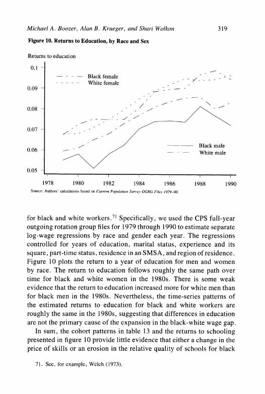
Michael A. Boozer, Alan B. Krueger, and Shari Wolkon 319
Figure 10. Returns to Education, by Race and Sex
Returns to education
0.1 - - - - - Black female - -
- - - - - White female 0.09-
0.08- /
,- 7' 0.07-
Black male 0.06 - White male
0.05 -
1978 1980 1982 1984 1986 1988 1990 Source: Authors' calculations based on Current Populatioui Surv'eY OGRG Files 1979-90.
for black and white workers.71 Specifically, we used the CPS full-year outgoing rotation group files for 1979 through 1990 to estimate separate log-wage regressions by race and gender each year. The regressions controlled for years of education, marital status, experience and its square, part-time status, residence in an SMSA, and region of residence. Figure 10 plots the return to a year of education for men and women by race. The return to education follows roughly the same path over time for black and white women in the 1980s. There is some weak evidence that the return to education increased more for white men than for black men in the 1980s. Nevertheless, the time-series patterns of the estimated returns to education for black and white workers are roughly the same in the 1980s, suggesting that differences in education are not the primary cause of the expansion in the black-white wage gap.
In sum, the cohort patterns in table 13 and the returns to schooling presented in figure 10 provide little evidence that either a change in the price of skills or an erosion in the relative quality of schools for black
71. See, for example, Welch (1973).

320 Brookings Papers: Microeconomics 1992
workers is responsible for the increase in the black-white earnings gap. More promising explanations for the increase in the gap are likely to involve structural factors examined by Bound and Freeman, such as the decline in unionization, the decline in the real minimum wage, and industrial shifts.
Conclusions and Policy Implications
This paper has assembled and analyzed a great deal of information regarding the quality of public schooling provided to black and white students since 1954. We draw six main lessons from our analysis.
First, wealth, not race, now seems to be the main determinant of the student-teacher ratio. Moreover, although black students have lower family wealth, on average, than do white students, nationwide both black and white students attend schools with roughly comparable pupil- teacher ratios. In the Northeast, however, class sizes are larger for the average black student than for the average white student. Hispanic students, on average, attend schools with a higher pupil-teacher ratio than do black or white students. The larger class size for Hispanic students results mainly from their high representation in the West.
Second, minority children are much less likely to be exposed to computers in school than white children, even after adjusting for family income. Minority children are also less likely than white children to use computers at home. Children from low-income families are less likely than those from high-income families to use computers in school.
Third, the decline in school segregation for black students in the South began on a wide scale around 1964, about 10 years after the Supreme Court's landmark decision in Brown v. Board of Education. Significantly, the movement toward integration began about 1964, 4 years before the Green decision, which required mandatory deseg- regation plans. The federal government's refusal to give funds to seg- regated school districts may have precipitated the movement toward integration.
Fourth, racial segregation in schools has been rising steadily for Hispanic students at least since 1968. Racial segregation in schools for black students has crept up in some regions and declined in others. Between 1968 and 1989, the Northeast moved from being the least

Michael A. Boozer, Alan B. Krueger, and Shari Wolkon 321
racially segregated region in the country to being the most racially segregated region for black students, and the South went from being the most racially segregated region to being the least. Moreover, black and Hispanic students in large, urban areas encounter extremely high levels of racial isolation.
Fifth, although far from conclusive, evidence suggests that students who use computers in the classroom are more likely to obtain jobs that require computer skills. Moreover, jobs that require the use of com- puters tend to pay more than jobs that do not require computer use. The widening gap in computer use between black and white workers could have accounted for at most one-third, and probably much less, of the increase in the black-white earnings gap between 1976 and 1990.
Sixth, between 1980 and 1990, the earnings gap between white and black workers expanded most for the 1950-59 cohort of workers, and least for the 1930-39 cohort. This finding is difficult to explain either by an erosion in school quality or by an increase in the price of skilled labor.
POLICY IMPLICATIONS. One obvious policy recommendation is that the government should enhance its effort to collect, and make publicly available, data on school resources by students' family income and race. Tracking the extent of racial segregation in urban areas should be a high priority. Information on the allocation of resources within schools by race also would be of great interest. The cost would not be exorbitant because much of the needed information is already collected but not disseminated or analyzed.
Second, many reports have recommended that schools promote sci- ence and mathematics education for minority students.72 We would add exposure to computers to this list. Real wages and employment op- portunities have expanded in sectors that require computer knowledge. Although preliminary, our results suggest that increasing students' use of computers in school enhances the probability that they will obtain a job that utilizes computers. Minority children are less likely to use computers in school. Specific remedies for increasing minority chil- dren's use of computers should be evaluated in relation to why the gap exists. Moreover, in view of the finding that workers with computer skills are more highly rewarded in the labor market than are workers
72. For example, see Quality Education for Minorities Project (1990).

322 Brookings Papers: Microeconomics 1992
without those skills, public sector job training programs might profitably seek to provide trainees with computer skills.
Finally, in light of evidence that we presented on the timing of school integration, we believe that the federal government's financial incen- tives for school integration beginning in the mid- 1960s were efficacious. Given the adverse consequences documented here and elsewhere of attending racially isolated schools, it may be wise for the federal gov- ernment to renew its efforts to provide school districts with an incentive to maintain racially balanced schools.
APPENDIX
Table A-1. Proportion of Black Students Who Attended All Black or Majority Black Schools in the Southern and Border States, 1924-71
All black Majority black Sample Year schools schools size
1924 0.953 1.000 70 1925 0.960 0.960 48 1926 1.000 1.000 66 1927 0.971 0.971 57 1928 0.897 0.931 46
1929 0.921 0.947 65 1930 0.955 0.955 39 1931 0.958 0.979 73 1932 0.880 0.920 40 1933 0.971 0.971 54
1934 0.974 1.000 52 1935 0.925 0.950 56 1936 0.922 0.961 67 1937 0.976 1.000 60 1938 0.947 0.974 62
1939 0.974 1.000 61 1940 0.930 0.977 62 1941 0.926 1.000 70 1942 0.903 0.952 75 1943 0.915 0.983 74
1944 0.944 0.963 66 1945 0.957 1.000 57 1946 1.000 1.000 54 1947 0.926 0.981 65 1948 0.981 1.000 68

Michael A. Boozer, Alan B. Krueger, and Shari Wolkon 323
Table A-1. (continued)
All black Majority black Sample Year schools schools size
1949 0.881 0.932 68 1950 0.930 1.000 71 1951 0.887 0.962 58 1952 0.903 0.952 75 1953 0.938 0.979 55
1954 0.883 0.950 74 1955 0.928 0.986 72 1956 0.910 0.955 76 1957 0.955 0.985 74 1958 0.880 0.960 79
1959 0.849 0.945 80 1960 0.924 0.962 81 1961 0.866 0.927 83 1962 0.869 0.976 90 1963 0.864 0.938 86
1964 0.796 0.888 102 1965 0.753 0.840 86 1966 0.656 0.823 97 1967 0.618 0.737 78 1968 0.500 0.711 79
1969 0.484 0.615 95 1970 0.329 0.588 88 1971 0.150 0.463 85
Source: Authors' calculations based on the National Survey of Black Americans.

324 Brookings Papers: Microeconomics 1992
Table A-2. Average Pupil-Teacher Ratios for Blacks, Hispanics, and Whites, by State, 1989
Number of
State Blacks Hispanics Whites schools
Alabama 19.09 19.25 19.73 1,287 Arizona 20.11 20.17 20.75 953 Arkansas 15.85 16.31 16.01 1,095 California 23.85 24.33 23.97 7,293 Colorado 17.67 17.87 18.77 1,301
Connecticut 15.08 15.46 14.78 966 Delaware 17.92 17.37 17.72 164 District of Columbia 18.10 16.97 18.55 182 Florida 17.87 18.77 18.19 2,217 Illinois 18.75 19.41 18.26 4,134
Indiana 18.31 19.17 18.63 1,855 Iowa 17.19 16.73 16.14 1,606 Kansas 17.90 17.00 16.17 1,455 Kentucky 17.74 18.30 18.10 1,359 Louisiana 17.38 17.51 17.39 1,460
Maryland 18.79 17.65 18.30 1,178 Michigan 17.17 15.94 15.70 3,266 Minnesota 18.47 17.92 18.32 1,487 Mississippi 19.14 19.05 19.13 873 Nebraska 17.47 16.59 15.73 1,475
Nevada 21.57 21.24 21.62 323 New Hampshire 17.54 18.30 16.98 443 New Jersey 15.11 15.13 15.13 2,237 New Mexico 19.03 18.72 19.27 654 New York 16.65 16.65 15.08 3,936
North Carolina 16.94 17.83 17.22 1,935 North Dakota 22.36 19.98 19.15 627 Ohio 18.16 18.93 19.64 3,683 Oklahoma 18.35 17.63 17.47 1,831 Oregon 18.98 19.38 19.38 1,188
Pennsylvania 17.14 16.83 16.80 3,165 South Carolina 17.27 18.15 18.07 1,045 Tennessee 19.98 20.08 20.06 1,499 Texas 17.06 17.78 16.97 5,780 Utah 23.44 23.45 24.78 708
Vermont 18.34 17.34 18.09 335 Washington 20.28 20.40 21.26 1,632 West Virginia 15.90 16.87 16.49 975 Wisconsin 17.51 17.47 16.63 2,008
U.S. 18.13 20.30 18.35 69,610 Source: Authors' calculations based on Common Core Public School Universe File. Survey does not include Alaska, Georgia,
Hawaii, Idaho, Maine, Massachusetts, Missouri, Montana, Rhode Island, South Dakota, Virginia, and Wyoming.

Michael A. Boozer, Alan B. Krueger, and Shari Wolkon 325
Table A-3. Students' Computer Use by State and Race
Percentage of students using computers at school Sample size
State All races Black White for all races
Alabama 38.7 36.4 39.1 274 Alaska 65.9 ... 66.5 340 Arizona 54.5 . . . 58.1 257 Arkansas 44.7 26.0 48.3 322 California 44.1 40.4 49.4 1,487
Colorado 65.6 . . . 65.9 276 Connecticut 51.9 ... 54.8 210 Delaware 41.9 32.8 45.3 234 District of Columbia 48.6 46.1 61.9 138 Florida 52.0 46.9 55.4 1,018
Georgia 51.5 46.3 54.9 340 Hawaii 57.9 . . . 58.1 95 Idaho 44.7 . . . 46.4 389 Illinois 52.8 31.0 62.0 1,024 Indiana 49.9 . . . 51.6 327
Iowa 62.2 ... 62.7 320 Kansas 66.3 ... 67.0 317 Kentucky 61.0 .. . 61.5 292 Louisiana 35.0 30.4 37.2 301 Maine 68.1 . . . 68.0 257
Maryland 47.2 42.5 50.4 212 Massachusetts 58.5 43.2 60.6 790 Michigan 51.2 39.6 53.1 983 Minnesota 71.6 ... 72.4 285 Mississippi 30.9 24.5 35.9 375
Missouri 56.0 ... 54.5 241 Montana 57.3 . . . 56.4 342 Nebraska 62.4 ... 61.6 327 Nevada 57.0 ... 57.5 249 New Hampshire 58.1 . . . 57.8 203
New Jersey 53.7 33.6 59.9 778 New Mexico 55.2 . . . 63.0 335 New York 52.7 46.0 57.7 1,362 North Carolina 54.4 43.4 57.9 949 North Dakota 62.3 . . . 62.5 326
Ohio 50.2 36.7 52.1 1,161 Oklahoma 52.8 . .. 54.6 288 Oregon 53.0 ... 53.6 249 Pennsylvania 56.9 40.0 59.0 925 Rhode Island 49.0 . .. 49.5 208
South Carolina 41.8 37.4 44.7 396 South Dakota 36.9 . . . 36.4 397 Tennessee 45.9 30.8 54.6 311 Texas 53.8 24.7 54.0 1,245 Utah 45.7 . . . 47.9 439

326 Brookings Papers: Microeconomics 1992
Table A-3. (continued)
Percentage of students using computers at school Sample size
State All races Black White for all races
Vermont 52.2 ... 53.0 185 Virginia 64.3 39.6 64.3 357 Washington 75.5 ... 75.9 245 West Virginia 53.1 . .. 53.4 309 Wisconsin 66.8 . . . 66.9 328 Wyoming 75.5 . . . 75.9 277
U.S. 52.7 39.3 56.4 23,295 Source: Authors' estimates based on the Current Population Survey, October 1989. We do not report estimates for states for
which there are fewer than 40 observations in the sample. The sample includes students enrolled in public and private schools.

Comments and Discussion
Comment by John C. Haltiwanger: This paper has something for everybody. It addresses not only the time pattern of black-white wage differentials but also related issues in terms of school-quality patterns. It addresses issues involving the rise in wage inequality that we have observed in the last few decades. It addresses issues regarding rising skill differentials and the hypothesis that this had been induced by skill- biased technical change. In particular, this paper examines the impact of an often-cited manifestation of the changing technology, the in- creased use of computers in the workplace. The paper certainly cannot be faulted for not addressing fundamental issues in labor economics and the overlap between labor and industrial organization.
What does the paper have to say on each of these issues? The paper documents the narrowing of black-white wage differentials through the 1970s and a somewhat surprising widening since that time. Further- more, as others have noted, the paper stresses that the widening in the 1980s seems to parallel rising skill differentials over this time.
The paper also documents the tremendous changes in school quality over the past century in terms of traditional measures, such as pupil- teacher ratios. Others have documented tremendous changes in mea- sures such as length of term.1 The paper documents the convergence of differences in school quality for whites and blacks in terms of these traditional measures, and if you look at the patterns, you see, in fact, that much of the convergence occurred through the 1960s. In the last two decades, on the basis of these traditional measures, school-quality differences between blacks and whites have been relatively small.
What have been the implications of this convergence for the changes in black-white wage differentials in the 1980s? Given that black-white
1. Smith and Welch (1986).
327

328 Brookings Papers. Microeconomics 1992
wage differentials have expanded in the 1980s with cohorts with, pre- sumably, higher quality schools-at least, from these traditional mea- sures-one key finding of the paper is that school quality, in terms of these traditional measures, cannot explain the expanding black-white wage differentials.
Where do computers fit into all this? The paper suggests that computers might be a modem measure of school quality. Evidence is presented that blacks have less access to computers in schools than do whites. The argument is that, while black students in predominantly black schools may have achieved parity in terms of traditional measures such as class size, this does not mean that all students have equal access to educational resources, and one metric of this is computers. Furthermore, in this paper and in some of the companion papers by Krueger, there is the finding that there is a wage premium for using computers at work. This is interpreted in this paper as a premium for having this skill.
Given the recentness of the computer revolution, the authors do not try to explain the rise in black-white wage differentials by the lack of computers at school. They suggest instead that this may be symptomatic of less resources and is a cloud on the future horizon.
What are we to make of all this evidence? One thing I think we clearly learn from this paper is that traditional measures, such as pupil- teacher ratios and length of school term, are not the key variables of interest that they once were. Clearly, these were important measures, through the 1960s, and substantial progress was made in reducing the gap between blacks and whites in terms of these measures.
This raises the question: What are the key variables today? Is it resources? Is it computers? Undoubtedly, the latter are important, but, in my view, this seems to miss some other fundamental aspects of school quality in the overall educational environment.
For any of us who live in an urban environment and have children in public schools or who just read the daily newspaper, it is clear that school-quality issues seem closely linked to neighborhood problems of gangs, drugs, violence, crime, teenage pregnancy, dropout rates, and parental involvement. The idea of neighborhood effects, associated peer effects, and parental involvement has received renewed focus in re- search by economists. Recent papers on these issues strongly suggest that the company one keeps has an important influence.2
2. Case and Katz (1991).

Michael A. Boozer, Alan B. Krueger, and Shari Wolkon 329
If these neighborhood effects are important for school quality, then this raises questions regarding the evidence on the convergence of school quality and the associated implications for wage differentials. This paper makes an important-and seemingly persuasive-point that ris- ing black-white wage differentials in the 1980s cannot be attributed to school quality since the differential rises more for the 1950-59 birth cohort than for the 1930-39 birth cohort, and the latter seemingly had inferior schools relative to the former. Further evidence is offered that the time series patterns of change in the return to education for blacks and whites are similar over the 1980s. If neighborhood effects are important, however, then one must ask whether the 1950-59 cohort really did have better schools than the older cohort.
I do not want to suggest that this emphasis on the idea of peer group and neighborhood effects negates the importance of resources; further- more, computers are clearly an interesting measure of resources. I think, however, that the paper does somewhat overstate the disparity. If you look at table 5, the gap by 1989 in computer access between blacks and whites is primarily among elementary school students. Black high school students and white high school students essentially have the same access to computers by 1989.
It does not seem that a lack of teachers or, for that matter, a lack of computers is a primary source of concern for school quality. The im- portant question raised by the paper is: how should school quality be measured? I am arguing that measures, such as how much time teachers can actually spend on teaching, how conducive the environment is for learning, whether education is viewed as a desirable achievement among one's peers, and the degree of parental involvement, are likely to be equally important, or even more important, than whether there is an Apple computer down the hall. In any event, this paper makes clear that further attention should be directed toward appropriate measures of school quality in the 1990s.
Now let us go back to computers and their influence in the workplace. Even if computers were not fundamental in the past, it is likely they will become increasingly important. An important question for school systems is how many resources should be devoted to computer-oriented learning and programming.
Here we turn to the relationship between wages and computer use. The paper presents evidence that links the use of computers at school to the use of computers at work. Further, the evidence shows
330 Brookings Papers. Microeconomics 1992
a connection between the use of computers at work and higher wages.
What are we to make of this? Clearly, there is a correlation here. The question, obviously, is how to interpret this correlation. First, as the authors note, there is the obvious question of causality. Is it simply the case that high-ability workers are more likely to use computers? I am not sure the authors fully reconciled this, although they certainly tried many different methods to deal with this issue.
Second, what is meant by "using a computer" presumably varies by occupation. For professionals, some of the use of computers seems to be driven by the use of things like electronic mail, and it is not clear that the use of E-mail is really the type of skill on which the authors are basing their arguments. Thus, the computer usage premium may reflect large national firm effects or senior executive effects-people who use E-mail a lot. Alternatively, there is some interesting evidence in companion papers by Krueger on clerical workers. It does make sense that clerical workers, who know sophisticated word processing and spreadsheet packages, probably do earn a premium for having those skills. Detailed controlling for occupation and for the nature of computer use is of fundamental importance in this context. One simple means to investigate this would be to interact the computer usage variable with occupation and then to investigate whether the premiums are linked to occupations where the story is the most plausible, at least in terms of the interpretation the authors are trying to give it.
A related explanation, in terms of the relationship between wages and computer usage, has to do with size wage differentials. Many of us have noted that there are substantial wage differentials depending on firm and plant size. In the work that Steve Davis and I presented last year, we noted that a significant portion of the rising increase in wage inequality is associated with increases in the size wage differ- entials over the last 20 years.3 We argued that size wage differentials reflected differences in skill mixes across small and large plants and that skill-biased technical change was a plausible explanation of the dramatic increases in size wage differentials.
This story fits in nicely here when one considers some new evidence presented in a recent paper by Dunne and Schmitz.4 They combined
3. Davis and Haltiwanger (1991). 4. Dunne and Schmitz (1991).
Michael A. Boozer, Alan B. Krueger, and Shari Wolkon 331
data from the Survey of Manufacturing Technology with plant-level data from the Longitudinal Research Database for the year 1987. They find that large plants are much more likely than small plants to have adopted advanced technology-computer-aided design, robotics, and just the use of computers in general in the workplace. They also find that controlling for technology adoption helps explain a substantial fraction of size wage differentials. Putting all this together suggests that large firms and plants have been adopting computer technology at a faster rate; and we already know that the wages of these workers have been rising.
Let me briefly sum up my reaction to the paper. I am more persuaded by the negative results in the paper than by the positive results. The documentation of the time series of traditional measures of school qual- ity, such as class size, makes it clear that these are no longer the key measures that they once were and cannot account for current trends in black-white wage differentials. Since traditional measures are not the answer, the question is: what is the answer? The suggestion here is that resources-and, particularly, computer resources-are the answer. I think there is some suggestive evidence that computer usage may be important. I am not persuaded that this is the fundamental factor for school quality or for black-white wage differentials.
Comment by Glenn Loury: I can be brief, since John Haltiwanger has already made a number of the points that had occurred to me and, sadly, a few that had not. This ambitious paper has pulled together a great deal of valuable information. For example, the authors' imaginative use of the National Survey of Black Americans (NSBA) data to develop a retro- spective measure of desegregation trends in the South is a novel contri- bution. Their finding that a dramatic reduction in racial separation in that region had already begun in 1964, before the Supreme Court had signif- icantly strengthened enforcement methods, is particularly important.
The authors seem to push two central themes relevant to policy of which I am as yet not convinced: (1) that the federal government should encourage greater integration of the public schools because of its alleged benefits to blacks; and (2) that greater access to computers in schools would result in significant productivity gains for students in their sub- sequent careers. The work reported here, premature and tentative as the authors acknowledge it to be, does not provide a sufficiently solid empirical basis upon which to rest such far-reaching conclusions.

332 Brookings Papers: Microeconomics 1992
The impact of segregation on blacks' labor market outcomes is not at all precisely measured here. The two-stage least squares estimates based on the NSBA data, in regressions explaining years of education and log wages, yield standard errors roughly one and a half times the size of the coefficients on the "proportion black in high school" vari- able. So we basically do not know how the racial composition of a black student's high school affects these important outcomes.
High school racial composition does seem important in predicting the racial composition of the college attended by black students. But one could easily account for this by noticing that blacks in cities where they constitute a significant fraction of high school students may also attend in large numbers public colleges in those cities.
Moreover, there are conceptual issues here that limit the extent to which policy-relevant conclusions can be drawn from the analysis. In effect, the authors are trying to infer the quality of an output (education) by observing the levels of some selected set of inputs, without any direct measure of the output's quality, without observing many of the other complementary inputs being employed, without any information on input prices, and without any idea of the objectives being pursued by the agents making decisions concerning input usage. That is to say, we do not really know what is going on within the schools, or within the school districts, where resource allocation decisions are being made.
For example, one fact that emerges from the paper is that the pupil- teacher ratio is much higher in the western states than in the rest of the country. Why? A recent discussion in the popular press speculated that, in California, this is due to the ways in which state and district decisions concerning school finance have been affected by the Serrano decision, which mandated equalization of district-level spending. One may won- der whether the differences between East and West in the quality of schooling are as great as the differences in pupil-teacher ratios suggest. One suspects that they are not and that other factor employment de- cisions, unobserved by the authors, are being taken that partially offset the effects of class size.
More generally, qualitative factors vary across individual schools and across districts-parental support activities, student peer group effects, administrative allocation of students to gifted and special ed- ucation programs, magnet school enrollment policies, teacher quality. While these factors cannot be measured by the authors, they are prob- ably important determinants of the quality of the educational experience.

Michael A. Boozer, Alan B. Krueger, and Shari Wolkon 333
The question is whether their omission biases the estimated effects of the factors that are observed here. The probable answer is "yes."
Consider the discussion of racial differences in the access to com- puters. Blacks are less likely to use computers at school and less likely to have access to them at home. Even if they have access, they are less likely than whites to use a computer at home, conditional on having access there. Using numbers from the paper, one calculates that roughly 85 percent of whites and 65 percent of blacks with computers at home are making use of them. Obviously, there is something going on that affects computer literacy other than the availability of the resource.
Indeed, the logic of the paper's argument seems to be that computer use in schools increases the likelihood that computers will be used at work, and/or that the student will end up working in an occupation where computers are used. The result of this causal chain is then an increase in the student's subsequent earnings. Notice, though, that the use of computers in schools usually does not involve the acquisition of computer skills, but rather is ordinarily a byproduct of some other educational purpose, often including remedial education.
Moreover, computer use at work is often done by people who have had no exposure to computers in schools, as the authors note, for the simple reason that they were educated before computers were widely available. For these reasons it is not at all clear that an intervention that leads to more widespread use of computers in schools will result in those affected enjoying higher earnings, notwithstanding the authors' finding that there is a correlation in the data between earnings and computer usage.
The general conceptual point is this: we are observing, in the ex- panding use of computers in schools and in the workplace, a dual diffusion process. As the nature of work and instruction is changed by the availability of this still evolving technology, computers are being adopted in both settings to accomplish a wider array of tasks. Twenty years ago few people used computers in school or at work; 20 years from now nearly everyone will be using them in both settings. By slicing into this process at a point in time, looking to the variation in usage and earnings in a cross-section, one is unlikely to derive useful infor- mation about the consequences for earnings of marginally increasing computer availability to some subset of students.
Racial comparisons are also problematic here. For complex reasons of social and occupational stratification, this dual diffusion may well

334 Brookings Papers: Microeconomics 1992
be advancing at different rates, and in different ways, for blacks and whites. Because an alteration in the disposition of computer resources does not alter these underlying facts of stratification, one may well wonder whether such a change will in fact lead to a narrowing of racial differences in earnings.
Authors' Response: John Haltiwanger and Glenn Loury have raised concerns that we have neglected neighborhood and peer effects. Al- though these potential influences on schooling outcomes are not ex- plicitly modeled in the paper, our analysis of school segregation is certainly one measure of the educational environment. Furthermore, because blacks in our sample were often exogenously constrained to attend segregated schools, school segregation is a feature of peer effects that is amenable to statistical analysis and inference. We also suspect that peer group effects were more conducive to learning for blacks born in the 1950s-who were among the first to attend integrated schools- than for earlier cohorts of blacks.
The discussants' caveats on our interpretation of computer use are well taken and worthy of further study. Loury, however, neglects our finding that students who use computers in school-for whatever purpose-are more likely to use computers at work. Nevertheless, we agree with Hal- tiwanger that lower computer use is not the "fundamental factor" for black-white wage differentials, but our analysis suggests that it is a con- tributing factor. And our evidence does not lead us to agree with Loury's prescription of allowing the "diffusion process" 20 years to repair racial differences in computer usage at school and work.
General Discussion: Both Timothy Bresnahan and Martin Neil Baily noted the irony of the authors' findings: computer usage in the workplace has a positive effect on wages; yet, it appears that the increased com- puterization of the workplace has still not resulted in a rise in U.S. labor productivity. While agreeing with the authors' findings that work- place computer usage differentials between blacks and whites explain part of their wage differentials, Bresnahan felt that computerization might be simply a proxy for rents to certain desirable jobs.
Frank Wolak and Paul Joskow both commented on the pupil-teacher ratios used by the authors. Wolak felt that the high pupil-teacher ratios found in western states might be attributed to rapid population growth in the cities of those states. He suggested that the authors put a control

Michael A. Boozer, Alan B. Krueger, and Shari Wolkon 335
for local population growth in their regressions that use pupil-teacher ratio and other city-related characteristics. Joskow was concerned about the accuracy of the pupil-teacher ratios, particularly the very high ratios for California. He wondered if large differences in pupil-teacher ratios across states were attributable to different methods used in calculating this measure; he suspected that administrators were being counted as teachers in some states, but not in others. Joskow suggested examining the correlation between pupil-teacher ratios and expenditures per pupil to see if the pupil-teacher ratios were really meaningful numbers.
Peter Reiss noted that the paper's message-that is, inputs into the school production function appear to be highly correlated with future wages of students-is not really race-based at all. He suspected that similar results would be seen by looking at gender. He suggested that the authors develop race-sex interactions by school input measures to see if these inputs can also explain male-female, black male-white male, and black female-white female wage differentials.
Zvi Griliches commented on the use of occupational data in earnings functions. He also noted that because occupations are so numerous, it is not possible to put them into an equation as dummy variables. Gril- iches said that sociologists have ranked occupations, converting each occupation to a numerical value (known as Duncan's SES scale). He said that in work he had done a long time ago, he had found a strong correlation between such a scale and wages. Thus, computer use in occupations may be just an alternative to such a scale.
Griliches also argued that it is not really clear what the output of a school is. School output is generally counted in years, but because schools differ in quality, they produce "different" years of schooling, he said. The quality issue is complex; schools are producing different products, which are priced differently by the economy.
Wolak was surprised that large-scale school desegregation began in 1964. He was interested in seeing an explanation for why this had occurred before the 1968 desegregation court case.

336 Brookings Papers: Microeconomics 1992
References
Ashenfelter, Orley, and Alan B. Krueger. 1992. "Estimates of the Economic Return to Schooling from a New Sample of Twins." Princeton University.
Behrman, Jere R., Zdenek Hrubec, Paul Taubman, and Terence J. Wales. 1980. Socioeconomic Success: A Study of the Effects of Genetic Endowments, Family Environment and Schooling. Amsterdam: North-Holland.
Blackburn, McKinley L., and David Neumark. 1991. "Omitted-Ability Bias and the Increase in the Return to Schooling." NBER working paper 3693. Cambridge, Mass.: National Bureau of Economic Research, May.
Blau, Francine D., and John W. Graham. 1989. "Black/White Differences in Wealth and Asset Composition." NBER working paper 2898. Cambridge, Mass.: National Bureau of Economic Research, March.
Bond, Horace Mann. 1934. The Education of the Negro in the American Social Order. New York: Prentice Hall.
Bound, John, and Richard Freeman. 1992. "What Went Wrong? The Erosion of Relative Earnings and Employment Among Young Black Men in the 1980s." Quarterly Journal of Economics 107 (February):201-32.
Braddock, Jomills H., II, Robert L. Crain, and James M. McPartland. 1984. "A Long-Term View of School Desegregation: Some Recent Studies of Graduates as Adults." Phi Delta Kappan 66 (December):259-64.
Card, David, and Alan B. Krueger. 1992a. "School Quality and Black-White Relative Earnings: A Direct Assessment." Quarterly Journal of Economics 107 (February): 151-200.
. 1992b. "Does School Quality Matter? Returns to Education and the Characteristics of Public Schools in the United States." Journal of Political Economy 100 (February): 1-40.
Case, Anne C., and Lawrence F. Katz. 1991. "The Company You Keep: The Effects of Family and Neighborhood on Disadvantaged Youths." NBER working paper 3705. Cambridge, Mass.: National Bureau of Economic Re- search, May.
Coleman, James S., Sara D. Kelly, and John A. Moore. 1975. Trends in School Segregation, 1968-73. Washington: The Urban Institute.
Coleman, James S., and others 1979. Equality of Educational Opportunity. New York: Arno Press.
Conlisk, John. 1971. "A Bit of Evidence on the Income-Education-Ability Interrelation." Journal of Human Resources 6 (Summer):358-62.
Crain, Robert, and Jack Strauss. 1985. "School Desegregation and Black Occupational Attainments: Results from a Long-Term Experiment. " Center for Social Organization of Schools, Johns Hopkins University.
Davis, Steve J., and John Haltiwanger. 1991. "Wage Dispersion Between and Within U.S. Manufacturing Plants, 1963-86." Brookings Papers on Eco- nomic Activity: Microeconomics 1991, 115-80.

Michael A. Boozer, Alan B. Krueger, and Shari Wolkon 337
Donohue, John H., III, and James J. Heckman. 1991. "Continuous Versus Episodic Change: The Impact of Affirmative Action and Civil Rights Policy on the Economic Status of Blacks." Journal of Economic Literature 29 (December): 1603-43.
Dubois, W. E. B., and Augustus G. Dill, eds. 1911. The Common School and the Negro American. Atlanta: Atlanta University Press.
Dunne, Tim, and James Schmitz. 1991. "Technology and Wages at U.S. Manufacturing Plants." Bureau of the Census. August 1991. Preliminary draft.
Dynarski, Mark. 1987. "The Scholastic Aptitude Test: Participation and Per- formance." Economics of Education Review 6:263-73.
Freeman, Richard B. 1973. "Changes in the Labor Market for Black Ameri- cans, 1948-72." Brookings Papers on Economic Activity 20:67-120.
Griliches, Zvi, and William M. Mason. 1972. "Education, Income, and Abil- ity." Journal of Political Economy, 80 (May/June):S74-S 103.
Hanushek, Eric. 1986. "The Economics of Schooling: Production and Effi- ciency in the Public Schools." Journal of Economic Literature 24 (Septem- ber): 1141-77.
Hochschild, Jennifer L. 1984. The New American Dilemma: Liberal Democ- racy and School Desegregation. New Haven: Yale University Press.
Jaynes, Gerald D., and Robin M. Williams, Jr. 1989. A Common Destiny: Blacks and American Society. Washington: National Academy Press.
Jones, Thomas Jesse. 1917. Negro Education: A Study of the Private and Higher Schools for Colored People in the United States (Office of Education, bulletin no. 38).
Juhn, Chinhui, Kevin M. Murphy, and Brooks Pierce. 1991. "Accounting for the Slow-down in Black-White Wage Convergence." In Workers and Their Wages: Changing Patterns in the United States, edited by Marvin H. Kosters. Washington, D.C.: American Enterprise Institute.
Katz, Lawrence S., and Ana L. Revenga. 1989. "Changes in the Structure of Wages: The United States vs. Japan." Journal of the Japanese and Inter- national Economies 3 (December):522-53.
Kozol, Jonathan. 1991. Savage Inequalities: Children in America's Schools. New York: Crown Publishers.
Krueger, Alan B. 1991. "How Computers Have Changed the Wage Structure: Evidence from Microdata, 1984-1989." NBER working paper 3858. Cam- bridge, Mass.: National Bureau of Economic Research, October.
Margo, Robert A. 1990. Race and Schooling in the South, 1880-1950: An Economic History. Chicago: University of Chicago Press.
McPhail, Irving P. 1985. "Computer Inequities in School Uses of Microcom- puters: Policy Implications." Journal of Negro Education 54 (Winter):3- 13.

338 Brookings Papers: Microeconomics 1992
Nechyba, Thomas J. 1990. "The Southern Wage Gap, Human Capital and the Quality of Education." Southern Economic Journal 57 (October):308-22.
Orfield, Gary. 1983. Public School Desegregation in the United States, 1968- 1980. Washington: Joint Center for Political Studies.
Quality Education for Minorities Project. 1990. "Education That Works: An Action Plan for the Education of Minorities." Cambridge, Mass.: Massa- chusetts Institute of Technology.
Ragosta, Marjorie, Paul W. Holland, and Dean T. Jamison. 1982. Computer- Assisted Instruction and Compensatory Education: The ETSILAUSD Study, The Final Report. Princeton: Educational Testing Service.
Schick, Frank L., and Renee Schick. 1991. Statistical Handbook on U.S. Hispanics. Phoenix, Ariz.: Oryx Press.
Smith, James P. 1984. "Race and Human Capital." American Economic Re- view 74 (September):685-98.
Smith, James P., and Finis R. Welch. 1986. Closing the Gap: Forty Years of Economic Progress for Blacks. Santa Monica, Calif.: RAND Corporation.
. 1989. "Black Economic Progress After Myrdal." Journal of Eco- nomic Literature 27 (June):519-64.
Welch, Finis R. 1973. "Education and Racial Discrimination." In Discrimi- nation in Labor Markets, edited by Orley Ashenfelter and Albert Rees. Princeton: Princeton University Press.
Welch, Finis R., and Audrey Light. 1987. New Evidence on School Deseg- regation. Los Angeles: Unicon Research Corporation.