UTILIZING MULTIPLE DATASETS FOR SNOW COVER MAPPING

Andrew B. Tait, Dorothy K. Hall, James L. Foster, Richard L. Armstrong

Statement of Significance

Global snow cover has a significant impact on the Earth's energy balance.Three methods are currently used to estimate snow cover on a large scale:interpolation of climate station data, mapping from satellite-attained optical data,and mapping from satellite-attained passive microwave (PM) data. Salomonsonet aL (1995) conclude that both optical and PM data should be used in synergy toprovide optimum results in snow cover mapping. Likewise, Barry et al. (1995)remark that no single sensor or methodology alone can provide all theinformation required. In this study, NOAA snow charts (NSCs), Special SensorMicrowave Imager (SSM/I) derived snow cover, and climate station snow depthdata are combined with additional climatic and surface elevation data to produce

an optimum snow-cover product for North America. Many of the problemsassociated with the optical and PM methods, when used alone, have beendiminished although the boreal forest remains a problem area. In addition, theMultiple Dataset Snow-Cover Product (MDSCP) provides more information onthe state of the snow cover with four snow-cover classes (fully covered, highelevation snow, patchy snow, and no snow) rather than two (snow and no snow.)

Relationship to MPTE Science Plan

This study presents a snow cover product that combines several sourcesof remotely-sensed and ground-based data. It addresses MPTE concernsregarding (1) algorithm development and (2) monitoring land-cover change.

Popular Summary

Integrating data from several sources to map global snow cover hasseveral advantages, as is shown in this study. First, snow is mapped irrespectiveof cloud cover due the inclusion of PM and station data. Second, thecombination of the NSC and station data reduces the PM errors of omission in

the spring caused by melting snow. Third, the MDSCP is a spatially completesnow-cover map for the end of the week, whereas the NSCs are composites overone to seven days while the PM-derived maps have sizeable swath gaps.Fourth, the MDSCP has four classes of snow cover (fully covered, thin or patchy,

https://ntrs.nasa.gov/search.jsp?R=19990092374 2018-08-28T13:18:14+00:00Z

ir

high elevation, or no snow cover) compared with the normal two (snow and nosnow), which provides more information about the state of the snow cover. Fifth,the percent snow-covered area has been calculated for each class based on ananalysis of the climate station data. These values are used to calculate the NorthAmerican snow-covered area with greater accuracy than in the past. Last, theMDSCP can be used operationally without station data, although some spatialinformation is lost.

The primary disadvantage with the MDSCP is poor resolution. Comparedwith the NSCs (cell size between 16,000 and 42,000km2), the EASE-grid SSM/Iand MDSCP cell resolution (628km 2) is significantly better. However, for the

purposes of mapping snow it is advantageous to have a resolution of less thanlkm. This would reduce the problem of not mapping snow in the boreal forestduring the late fall / early winter, as only the very densely forested stands wouldobscure the under.lying snow. MODIS-derived daily global snow-cover maps,with a resolution of 500m, will be available for the 1999 / 2000 snow season.With this resolution, it is foreseeable that these optical data will be used as theprimary source of snow-cover information, rather than the passive microwavedata, except over areas with thick cloud cover. In the year 2000, EOS PM-1AMSR-derived snow-cover maps will also be available, at a resolution of 12.5km.

Barry, R.G., Fallot, J-M., and Armstrong, R.L. (1995), Twentieth-centuryvariability in snowcover conditions and approaches to detecting andmonitoring changes: status and prospects. Progress in PhysicalGeography, 19(4):520-532.

Salomonson, V.V., Hall, D.K., and Chien, J.Y.L. (1995), Use of passivemicrowave and optical data for large-scale snow cover mapping.Proceedings of the 2 nd Topical Symposium on Combined Optical-Microwave Earth and Atmosphere Sensing, Atlanta, GA, April 3-6, 1995,35-37.

=i,,w _w

Utilizing Multiple Datasets for Snow Cover Mapping

A.B. Tait

Universities Space Research Association, 7501 Forbes Blvd., Suite 206,

Lanham, MD 20706

D.K. Hall

J.L. Foster

Hydrological Sciences Branch, Mail Code 974, NASA/Goddard Space Flight

Center, Greenbelt, MD 20771

R.L. Armstrong

National Snow and Ice Data Center, Campus Box 449, University of Colorado,

Boulder, CO 80309-0449

Paper submitted to

Remote Sensing of Environment

June 1999

Address correspondenceto A.B. Tait, Mail Code 974, NASA/GSFC, Greenbelt,

MD 20771.

ABSTRACT

Snow-cover maps generated from surface data are based on direct

measurements, however they are prone to interpolation errors where climate

stations are sparsely distributed. Snow cover is clearly discernable using

satellite-attained optical data because of the high albedo of snow, yet the surface

is often obscured by cloud cover. Passive microwave (PM) data is unaffected by

clouds, however the snow-cover signature is significantly affected by melting

snow and the microwaves may be transparent to thin snow (< 3cm). Both optical

and microwave sensors have problems discerning snow beneath forest

canopies.

This paper describes a method that combines ground and satellite data to

produce a Multiple-Dataset Snow-Cover Product (MDSCP). Comparisons with

current snow-cover products show that the MDSCP draws together the

advantages of each of its component products while minimizing their potential

errors. Improved estimates of the snow-covered area are derived through the

addition of two snow-cover classes ("thin or patchy" and "high elevation" snow

cover) and from the analysis of the climate station data within each class. The

compatibility of this method for use with Moderate Resolution Imaging

Spectroradiometer (MODIS) data, which will be available in 1999, and with

Advanced Microwave Scanning Radiometer (AMSR) data, available in 2000, is

also discussed. With the assimilation of these data, the resolution of the MDSCP

would be improved both spatially and temporally and the analysis would become

completely automated.

1. INTRODUCTION

When snow covers the ground the exchange of energy at the surface is

altered radically. Snow has a very high albedo (0.40 to 0.95) compared with soil

2

(0.05 to 0.40) and vegetation (0.05 to 0.26). Due also to its high thermal

emissivity and low thermal conductivity, snow cover strongly influences the

overlying atmosphere (Chang et aL, 1985). It has been suggested that

anomalies of the snow cover may induce complex feedback mechanisms leading

to local and global climate fluctuations (Hahn and Shukla, 1976; Walsh and

Ross, 1988). In addition, snow cover is an essential component of the global

hydrological cycle.

Because of the influence of snow on weather and climate, and the need to

know where and how much snow exists, some investigators have used

interpolation techniques to project snow-cover information obtained at climate

stations to a larger area. Brown and Braaten (1998) used daily snow-depth

measurements from approximately 3000 sites to estimate the snow cover over

Canada. Even with this many stations, though, large areas in the Northwest

Territories were considerably undersampled. Knowledge of the global snow-

covered area from surface-based measurements is similarly limited due to large

gaps in the recording networks in both space and time. It is therefore important

to develop alternative techniques to remotely observe the global distribution of

snow cover.

NOAA has produced satellite-derived end-of-the-week snow-cover maps

for the whole of the Northern Hemisphere since 1966 (Matson et al., 1986;

Robinson et aL, 1993). These maps are important for monitoring the snow cover

at the continental to global scale. Consequently, they are vital for improving

large-scale hydrological models, refining medium- and long-range weather

forecasts, and for fine tuning general circulation models (Rango, 1985). In

addition, long-term changes in snow cover may indicate responses to climate

change (Barry, 1985).

The NSCs are derived from satellite-attained reflected visible radiation

data in the wavelength range 0.55 to 0.75 microns. The satellites used for the

identification of snow are the Geostationary Operational Environmental Satellites

(GOES), the Meteosat, the Geostationary Meteorological Satellite (GMS) and the

NOAA polar-orbiting satellites. Snow is discriminated from cloud by observing

3

cloud movement and by identifying surface features such as mountain ridges and

river valleys. If a region is completely obscured by cloud then the analyst goes

back to the last day that the surface can be seen (Robinson et aL, 1993). Last,

the hand-drawn maps are digitized on to an 89 by 89 cell Northern Hemisphere

grid with cell sizes ranging from 16,000 to 42,000km 2.

The NOAA National Environmental Satellite, Data, and Information

Service (NESDIS) updated the snow cover mapping procedure in 1997 with the

interactive multi-sensor snow and ice mapping system (IMS). The new maps

take less time to prepare, are fully digital and are produced daily (Ramsay,

1998). In this study however, only the end-of-the-week NOAA snow-cover maps

are used.

Satellite-attained PM data are used to estimate the snow-covered area

when the snowpack is dry, as there is sufficient contrast in the brightness

temperature range between snow and bare ground due to a lower dielectric

constant and the effect of scattering in snow (Chang et aL, 1976; Rango et al.,

1979). The onset of melt, however, transforms a snowpack from one that

scatters microwave radiation to one that absorbs and re-emits it (Ulaby and

Stiles, 1980). This dramatically increases the brightness temperature (TB) to that

approaching the physical temperature of the medium and makes snowfield

monitoring more difficult. For this and other reasons, it has been suggested by

several authors that PM data should be used in conjunction with visible and near-

infrared data for the determination of snow-covered area (Foster et aL, 1984;

Robinson et aL, 1993).

Grody and Basist (1996) developed a decision tree method for identifying

snow cover using PM data from the Special Sensor Microwave/Imager (SSM/I).

Their approach uses filters derived from microwave scattering theory (Chang et

al., 1976; Ulaby et al., 1982; Stogryn, 1986) and field experiments (Hall et al.,

1984; M&tzler and Huppi, 1989; Neale et al., 1990; Grody, 1991)to separate the

scattering signature of snow from the scattering signatures of precipitation, cold

deserts, and frozen ground. A comparison between the NSCs and SSMll-

derived snow maps averaged over the current and adjacent weeks showed that

4

the PM method maps slightly less snow, but the difference was no more than

3%. This was attributed to different temporal sampling (the NSC map is an end-

of-the-week product, while their SSM/I mapwas averaged over the whole week),

and the SSM/I's reduced sensitivity to shallow dry snow and melting snow (Basist

et aL, 1996).

Three methods have been described above that are currently used to

estimate snow cover on a large scale: interpolation of climate station data,

mapping from satellite-attained optical data (the NSCs), and mapping from

satellite-attained PM data. Each method has problems, however, and these and

their effects are summarized in Table 1. Salomonson et al. (1995) conclude that

both optical and PM data should be used in synergy to provide optimum results

in snow cover mapping. Likewise, Barry et al. (1995) remark that no single

sensor or methodology alone can provide all the information required.

In this study, the above data are combined with additional climatic and

surface elevation data to produce an optimum snow-cover product for North

America. This paper describes in detail the datasets and the methodology used

to fulfill this objective. The new maps are compared with NSC and PM-derived

snow-cover maps as well as with several NOHRSC snow-cover maps.

Estimates of the North American snow-covered area are also produced. Last,

we consider whether this approach can be used with Earth Observing System

(EOS) MODIS and AMSR data, and whether the maps can be produced

operationally. MODIS is scheduled to be launched in 1999 aboard EOS Terra

and AMSR is scheduled to be launched in 2000 aboard EOS PM-1.

2. DATA

The following datasets, projected to the National Snow and Ice Data

Center (NSIDC) 25-km Equal Area Scalable Earth (EASE) Northern Hemisphere

grid (with the exception of cloud cover), were used in this analysis. Only data for

North America were used as only those climate station data were obtained.

5

• NOAA digitized snow-cover charts (NSCs) derived from Advanced Very High

Resolution Radiometer (AVHRR) and GOES data (distributed on CD by

NSDIC);

• The Grody and Basist (1996) PM snow-cover product (which uses a decision

tree method employing SSM/I data);

• Climate station snow-depth data from the USA and Canada;

• Navy maximum and minimum surface elevation data;

• Surface mean daily air temperature data obtained from the NOAA Climatic

Diagnostics Center (CDC); and

• Cloud cover inferred from the NSCs (the dates written on the maps establish

the day when the area was last cloud-free).

Figure 1 shows the locationof the climate stations used in this study. The

Canadian data were obtained from the Atmospheric Environment Service (ca.

3000 stations) and data from over 8000 stations within the United States were

obtained from the National Climatic Data Center. A station location is defined as

snow covered when the recorded snow depth is greater than or equal to lcm.

It was deemed necessary to segregate terrain based on geomorphic

complexity. This is because snow cover over complex terrain is less contiguous

than over flat regions. Using the Navy maximum and minimum elevation data,

the surface was divided into complex and non-complex terrain (Figure 2). Each

EASE-grid pixel (25 by 25km) was classed as "complex" if the difference

between the maximum and minimum elevation within the pixel is greater than

500 meters. This cutoff was chosen to best concur with known regions of

mountainous terrain.

The period of analysis for this study, August 1987 through July 1995, was

determined by the availability of the digitized NSCs in EASE-grid format

(obtained from the Weekly Snow Cover and Sea Ice Extent CDs). The period of

this analysis will be extended through May 31, 1999 when the CDs are updated.

After this date, the weekly NSCswill be discontinued and only the daily product

6

will be produced. The EASE-grid SSMII brightness temperature data were also

obtained from NSIDC. Due to instrument problems however, there are periods

when either no PM data are available, a specific channel is out, or the data

coverage is severely limited. Table 2 shows the days corresponding to the end-

of-week NSCs between August 1987 and July 1995 when the SSM/I data is

limited.

3. METHODS

This study uses a series of decisions that determines where and when

snow should be mapped. In addition to mapping pixels as "snow covered" or

"snow free," two other snow classes are produced. These are "thin or patchy"

and "high elevation" snow cover. In general, the snow cover is considered "thin

or patchy" when the satellite maps and station data disagree in areas of non-

complex terrain. Thus, parts of the pixel may be snow covered while parts are

snow free, or the snow cover may be thin (< 3cm). "High elevation" snow cover

is similarly classified for areas of complex terrain, but it implies that the pixel is

snow free at lower elevations and snow covered at high elevations. The input

data for the analysis are the Grody and Basist (1996) PM snow-cover maps, the

NSCs, surface air temperature, surface complexity and cloud cover.

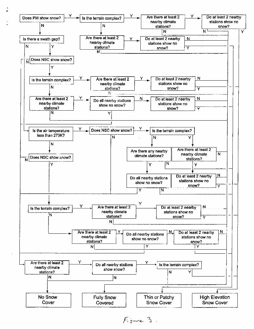
Figure 3 is a decision tree diagram that describes the snow-cover

classification procedure. To simplify the decision tree, sky conditions are

assumed cloudy. A final, manual step (not shown in Figure 3) modifies the snow-

cover product in areas of no or little cloud. The PM map is used as a starting

point for the analysis. This is because the Grody and Basist (1996) algorithm

filters out much of the scattering signatures caused by precipitation, cold deserts,

and frozen ground. The main problems that remain are caused by wet snow,

dense forests, and thin dry snow. All of these sources of error are errors of

omission and lead to a potential underestimation of snow cover. It is reasonable,

therefore, to use the PM-derived snow-cover map as the probable minimum

7

snow-covered area at this resolution. Thus, an EASE-Grid pixel mapped as

snow covered by the PM method is likely to have snow on the ground, which

makes this a good starting point for the analysis. Comparisons of the PM data

with climate station, NSC, air temperature, and surface roughness data

determine the snow-cover class of each pixel: "fully snow covered", "thin or

patchy" snow cover, or "high elevation" snow cover.

In PM swath gaps the NSC data are used as the primary source of snow-

cover information and are modified, if necessary, by the ground data. In areas

within the SSM/I swaths, where the NSC map shows a more extensive snow

cover than the PM map and the air temperature is greater than 273K, the NSC

snow cover not mapped by the PM method may be melting. In this situation, the

NSC map is probably more accurate than the PM map, and is used as the

primary data source. When the NSC map shows a more extensive snow cover

than the PM map and the air temperature is less than 273K, the NSC snow cover

may be thin, or if there are clouds present, it may have been misidentified. In this

case, the PM snow cover is given priority.

If both satellite-derived maps show "no snow" and the nearby climate

stations unanimously show "snow" (there must be at least two nearby stations),

the snow cover may be dirty and wet or tall vegetation may be obscuring the

snow cover from the view of the satellites. In this situation, snow cover is

mapped based on the ground data alone.

Last, cloud cover information is manually gleaned from the hand-drawn

NSCs. If an area is obscured by cloud on the last day of the week, the analyst

uses data for that region from a previous day. The date corresponding to the

cloud-free scene used to map the snow is marked on the map. Thus, if the date

corresponds to the last day of the week, then the area was cloud free for at least

some of that day. Under these conditions, the NOAA snow cover map is

considered more accurate than if it were cloudy and a previous day's data were

used. Given this assumption, two modifications (not shown in Figure 3) are

made to the snow-cover product for areas of no or little cloud.

8

First, if the cloud-free area is non-complex and the PM map shows "snow"

while the NSC shows "no snow," then any "fully snow-covered" pixels are

reclassified as "thin or patchy." Second, if there is a PM swath gap and the NSC

shows "snow" while nearby climate stations unanimously report "no snow," then

any pixels classified as "no snow" are reclassified as "thin or patchy" snow cover.

Both changes depict an increase in the confidence of the satellite-attained optical

data. These are the only changes from the decision tree that need to be made

given cloud-free conditions.

4. RESULTS

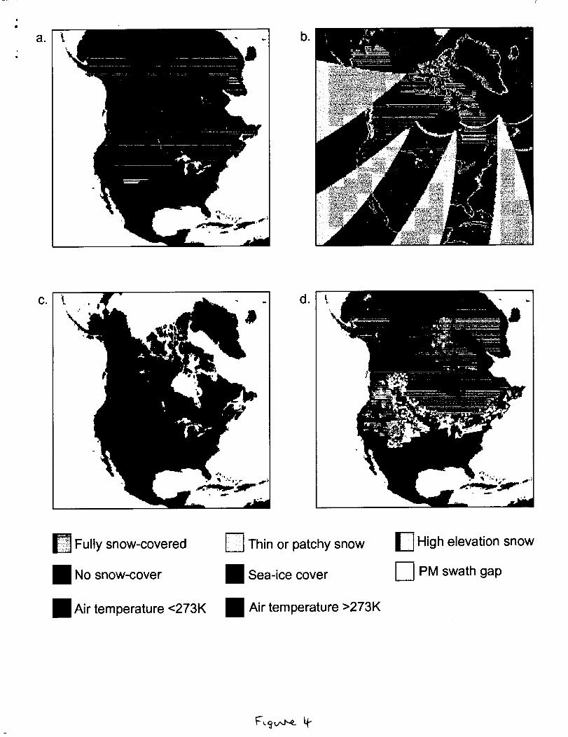
Figure 4 shows the NSC for the week April 2-9, 1995, and the PM-derived

snow-cover map, the surface air temperature freezing line and the MDSCP for

April 9, 1995. The main difference between the MDSCP and the NSC and PM

maps is the inclusion of the "thin or patchy" and "high elevation" snow-cover

classes. As these classes are determined principally by climate station data,

their occurrence in areas of sparse ground data coverage is rare. Hence, care

should be taken when interpreting the spatial pattern of the snow-cover classes.

Despite this, the inclusion of these classes significantly enhances the

interpretation of snow cover in the dense climate station areas and is therefore

highly beneficial for snow cover analyses.

From the example in Figure 4, two other differences between the MDSCP

and the input satellite-derived products that highlight the improvements in the

new product can be seen. First, the NSC shows snow from the Great Lakes

northwest through Minnesota, North Dakota and Saskatchewan while the PM

map shows this as snow free. Since the surface air temperature is below 273K

for this area, and since climate stations unanimously show no snow, the MDSCP

maps it as snow free. It is likely therefore, that the NSC is overestimating the

snow cover here, probably due to the presence of extensive cloud cover.

Second, the PM map shows no snow east of Lake Erie while the NSC maps

9

snow. The air temperature freezing line runs through this area. Where the

temperature is above 273K the snow may bewet, which can cause the PM

method to underestimate snow. The MDSCP maps this area as "thin or patchy"

snow because there are mixed reports of snow and no snow from the climate

stations in the area. Where the temperature is less than 273K, the MDSCP

maps no snow in accordance with the PM and station data. Here, as in the mid-

west, cloud cover may have led to an overestimation of the NSC snow cover.

Figure 4 shows, therefore, that the MDSCP is a weighted composite of the

input satellite and ground-based data. Moreover, the weights are based on the

relative degrees of confidence in these data. A problematic area is the North

American boreal forest. Here, confidence in both satellite-derived datasets is

relatively low (Table 1) while station data are sparse. Consequently, confidence

in the MDSCP in this region is also low. Upon inspection of the eight years of

data, both the NSCs and the PM snow-cover maps, and hence the MDSCP, may

be underestimating the snow cover in the boreal forest, particularly in the late fall

to early winter.

For example, in 1987 half of the climate stations in the boreal forest of

Ontario, Manitoba and Saskatchewan (14 of 30) reported snow on October 25.

Both the NSC and the PM snow map show continuous snow cover north of the

taiga/tundra border, though both map no snow within the forest. The situation is

the same on November 1 (15 of 30 stations). By November 8, both satellite

methods are mapping some snow in the forest, although the station data suggest

that the snow cover is more extensive (23 of 30 stations report snow). On 22

November the NSC completely fills in the forest as fully snow covered while the

PM-based method still shows patchy snow. The NSC "jump" in snow-covered

area is probably in response to snow south of the forest, as the NOAA analysts

commonly "fill in" the area north of the snowline as snow covered.

The pattern described above recurs every October. In 1991 in fact, the

NOAA analyst has written "Estimated Boundary" through the North American

boreal forest on October 27. This confirms that it is very difficult to map snow

cover from space in this region, particularly when the snowline is proceeding

10

south in the early winter. Currently the MDSCP does not improve on the NSC or

PM snow-cover maps for this region and season as all the input datasets have

problems. However, the errors associated with this problem should be reduced

when higher resolution MODIS (500 m resolution) and AMSR (12.5 km

resolution) products become available. The assimilation of these data is

discussed later.

Validation of the MDSCP is difficult, since the input datasets are those that

the product would be compared with (NSCs, PM snow-cover maps and climate

station data). In addition, withholding ground data from the analysis for the

purposes of validation is undesirable, as the more station data in the analysis,

the more accurate the product. One product that is not used as input however,

which can be used for comparison purposes, is the NOHRSC snow-cover

product. NOHRSC has developed and implemented a snow classification

algorithm that is used to classify both GOES and AVHRR imagery (Carroll,

1995). The non-automated algorithm is a multi-spectral, physically based

classifier that isolates snow from cloud and from all other surfaces. Several

weekly snow-cover composites, produced for the contiguous United States, were

compared with the MDSCP. Results showed that the maps are similar, despite

the different resolution (lkm versus 25km), integration period (weekly versus

daily) and projection (Lambert Equal Area versus EASE-grid).

An example of a NOHRSC / MDSCP comparison is shown as Figure 5.

The NOHRSC map is a composite over the period January 14-18 while the

MDSCP represents the snow cover on January 15, 1995. Aside from a

difference in the snow cover in the Nebraska panhandle - eastern Wyoming

region (NOHRSC maps snow while the MDSCP does not), the two maps agree

very well. Upon inspection of the ground data from western Nebraska and

eastern Wyoming, it was found that few climate stations reported snow (4 of 96

stations) throughout the period January 14-16, 1995. On January 17 and 18,

1995 however, many more stations in this region reported snow (65 of 96

stations). Hence for January 15, the MDSCP represents the snow cover more

accurately than does the NOHRSC 5-day composite.

11

With the inclusion of the "thin or patchy" and "high elevation" snow-cover

classes, the MDSCP provides more information about the state of the snow

cover than any of the current satellite-derived products. It is necessary to

quantify these classes with respect to their typical percent snow cover so that the

continental snow-covered area may be calculated. This is accomplished by

calculating the mean percent of climate stations within each snow-cover class

that is reporting snow. The analysis was performed for the winter months

(December through February - to ensure adequate snow coverage) over the

entire 8-year period, 1987-1995, and was repeated for "thin or patchy snow,"

"high elevation snow" and "fully snow-covered" areas. The results are presented

in Table 3.

The mean number of stations perwintertime snow-cover map in each

class is sufficiently high to use the mean percent of stations with snow cover as a

proxy for the mean percent snow cover within each class. From Table 3

therefore, the mean percent snow cover for "thin or patchy" snow pixels is 34.3%.

This value makes sense, as with around 34% of the pixel covered with snow the

satellites may detect enough snow to map the pixel as snow covered while the

station data may disagree.

The mean percent of stations reporting snow in areas of "high elevation"

snow cover is 24.6%. However, this does not represent the mean percent snow

cover. When a station reports no snow in an area of complex terrain where the

MDSCP shows "high elevation" snow cover, then it is assumed that while the

valleys may be snow free there is snow at higher elevations. To derive a mean

percent snow cover for the "high elevation" class, it is assumed that a pixel has

100% snow cover when a station reports snow and 50% snow cover when a

station reports no snow. These values have not been validated, although an

investigation comparing 30m Landsat TM data to the MDSCP is planned. The

percent snow cover in a "high elevation" snow-cover pixel is calculated as

follows:

%SCHE= 24.6 + (100 -- 24.6)*0.5

= 62.3%

12

The climate station analysis was also performed for areas classified as

"fully snow covered." It is unrealistic to assume that any 625 square kilometer

area is 100% snow covered, with the exception of Greenland and the Antarctic.

Local topographic (in general, slopes greater than 50 ° cannot retain snow) and

vegetative variability, in combination with the re-distribution of snow by wind,

result in areas of snow-free land even in regions that have snow cover for over

half of the year. Recent work by Hall et aL (submitted) for four different areas in

North America show that SSM/I pixels classified as 100% snow covered are

actually 70 to 72% snow covered when mapped using 30m resolution Landsat

TM data. The mean percent snow cover of the MDSCP "fully snow-covered"

pixels from the analysis of climate station data is 75.4 (Table 3). This agrees well

with the Landsat TM analysis results.

As the majority of climate stations are located south of around 55°N

(Figure 1), the percent snow cover estimates may be biased. It is conceivable

that the percent of snow cover in "fully snow covered" pixels in high latitudes is

much higher than 75%, for example. To test this hypothesis, data from Alaska

and the Canadian Northwest Territories were isolated and analyzed. The mean

percent of stations reporting snow in "fully snow covered" pixels for the period

1987 through 1995 was 68.8%, with a mean number of stations of 171, and a

mean standard deviation of 6.18. The percent snow cover is lower than when all

the data are used, however the standard deviation is higher (the result of a lower

sample size). Overall, it can be said that there is no evidence to suggest a

change in the percent snow cover with latitude.

The percent snow cover for the three snow classes are estimates based

on a limited number of climate station data. A study incorporating many Landsat

TM scenes, or other data of relatively high resolution such as from MODIS, for

each snow-cover class is required to validate these percent snow cover values.

Nevertheless, it is considered at present that the use of these percent snow

cover values is more realistic than assigning each snow-covered pixel a value of

100%.

13

A time series plot of North American snow-covered area (including

Greenland) derived from the NSCs and the MDSCP is shown as Figure 6. The

mean percent snow cover for each of the MDSCP classes has been used in the

calculation of the MDSCP snow-covered area, with the exception of Greenland

where the pixels are considered to be 100% snow covered. The difference

between the two datasets is up to 5.3 million square kilometers in winter. This is

due to the NSCs mapping snow-covered pixels as 100% while the MDSCP maps

these pixels as either 75%, 62%, 34% or 0% snow covered, contingent upon the

snow-cover class. Because the number of snow-covered pixels is greatest in

winter, and as the winter snowline is in an area of high climate station density

(hence more pixels are classed as "thin or patchy" or "high elevation" snow

cover), this is the season of greatest difference in the estimated North American

snow-covered area.

The difference between the NSC- and MDSCP-derived snow-covered

area is relatively consistent from year to year. The mean difference, along with

the standard deviation, is shown in Figure 7. The variability is greatest in late fall,

as this is the period of rapid transition of the snow-covered area. On average

over the year, though, the variability is quite low at around half a million square

kilometers or less. It is suggested, therefore, that the long time series of NSC-

derived snow-covered area (1966 onwards) could be amended using the mean

difference curve shown in Figure 7, yielding a 30-year time series of data for

North America based on the results of this analysis.

Over the period 1987-1995 the availability and condition of the SSM/I

brightness temperature data varies (Table 2). Between February 1, 1989 and

December 31, 1991 there were no data from the 85GHz channel due to

degradation of the instrument by solar illumination (Wentz, 1992). The PM-

derived snow-cover maps included in the MDSCP analysis were produced

without 85GHz data during this period. To test the sensitivity of no 85GHz data,

SSM/I and MDSCP maps were produced with and without the 85GHz channel for

the period September 27, 1992 through May 9, 1993. This snow season was

chosen because there is only one day when the PM data are missing and only

14

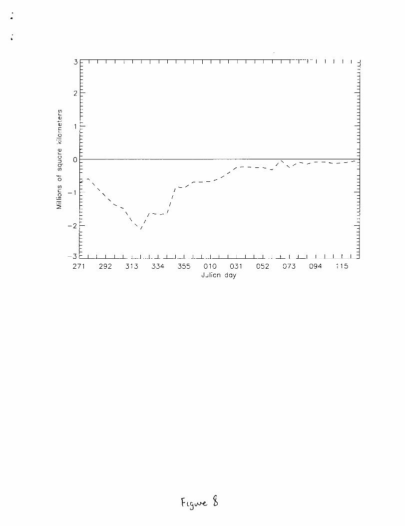
two days when the coverage is poor (Table 2). Figure 8 shows that the North

American snow-covered area derived from SSM/I data without the 85GHz data is

up to 2 million square kilometers less than that with the 85GHz channel in late

fall. The difference decreases through the winter as the snowline stabilizes and

the area covered by thin snow (< 3cm) is reduced (the 85GHz channel is

sensitive to thin snow.) In spring, the difference further decreases as the PM/

data is adversely affected equally at all frequencies by the presence of liquid

water.

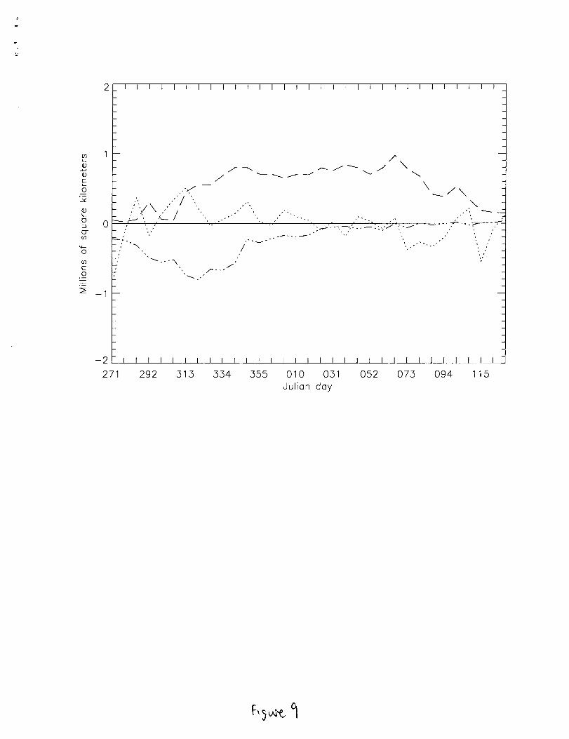
The snow-covered area for the 1992/1993 period derived from the

MDSCP with all the input data, without the SSM/I 85GHz channel, without any

SSM/I data, and without any climate station data is shown as Figure 9. The

effect of no 85GHz data in the MDSCP analysis is around 800,000km 2 in the late

fall. Thus, the MDSCP maps are less sensitive by a factor of two to the loss of

the 85GHz channel, compared with the PM-derived snow-cover maps. The "no

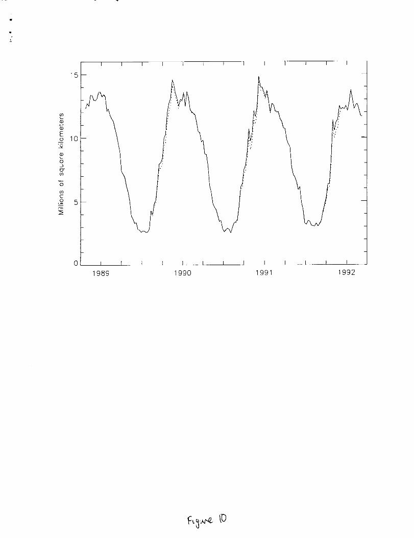
85GHz" curve from Figure 9 was smoothed with a 4-week moving average and

used to correct the North American snow-covered area time series during the

period February 1989 through December, 1991. The uncorrected and corrected

time series are shown in Figure 10.

A sensitivity test was also performed to observe the effect of no PM data

on the MDSCP. From Figure 9 it can be seen that the effect is largest when the

snowline is in transition in the fall and spring. During these seasons, however,

there is no pattern to the difference between using and omitting the PM data,

hence no correction to the data has been made. Last, a test was performed to

interpret the influence of omitting all the climate station data from the analysis

(Figure 9). If the MDSCP is to be used operationally, it may not be possible to

assimilate the station data in a timely fashion. The effect on the snow-covered

area increases steadily over the fall to a constant difference of around 800,000

km 2 throughout the winter, and then falls off steadily during the spring. This is

because while the location of snow-covered pixels is generally unchanged, many

fewer pixels are classified as "thin or patchy" and no pixels are classified as "high

elevation" snow cover when climate station data are not used. The effect is more

15

noticeable in the winter because the number of pixels classified as "thin or

patchy" or "high elevation" snow cover is greater when the snowline is at lower

latitudes.

Despite a loss of information about the state of the snowpack, an

adjustment to the total snow-covered area can be performed, as the pattern

caused by omitting the climate station data is highly regular (Figure 9). Thus, the

MDSCP can be used operationally for the purposes of calculating the snow-

covered area, particularly if a satellite-derived surface air temperature dataset is

used. Also, if the snow cover is mapped with a binary discriminator, i.e. snow

covered or snow free, then the inclusion or omission of climate station data

makes only a negligible difference.

5. DISCUSSION

Grody and Basist (1996) conclude that the majority of the errors

associated with the PM-derived snow-cover map appear on the "conservative"

side. Therefore, given problematic conditions such as melting or thin dry snow,

dense forest cover, or precipitation events, the PM snow-cover map may show

less snow than is present. The main error of commission is the misclassification

of frozen ground as snow cover, however this is mostly accounted for in their

filtering scheme. Hence, in all likelihood, if an EASE-Grid pixel is mapped as

snow by the PM method there is snow on the ground.

This acknowledgement yields a conservative map of the snow cover at

this scale, and hence, a starting point for a multiple-dataset analysis. Using the

elevation data and information from nearby climate stations, the snow-cover

class can be identified. Next, the NSC data are analyzed, in conjunction with air

temperature, elevation, and climate station data, to determine whether any

additional pixels should be classed as snow covered.

This method has several advantages. First, snow is mapped irrespective

of cloud cover due the inclusion of PM and station data. Second, the

16

combination of the NSC and station data reduces the PM errors of omission in

the spring caused by melting snow. Third, the MDSCP is a spatially complete

snow-cover map for the end of the week, whereas the NSCs are composites over

one to seven days while the PM-dedved maps have sizeable swath gaps.

Fourth, the MDSCP has four classes of snow cover (fully covered, thin or patchy,

high elevation, or no snow cover) compared with the normal two (snow and no

snow), which provides more information about the state of the snow cover. Fifth,

the percent snow-covered area has been calculated for each class based on an

analysis of the climate station data. These values are used to calculate the North

American snow-covered area with greater accuracy than in the past. Last, the

MDSCP can be used operationally wfthout station data, although some spatial

information is lost.

The primary disadvantage with the MDSCP is poor resolution. Compared

with the NSCs (cell size between 16,000 and 42,000km2), the EASE-grid SSM/I

and MDSCP cell resolution (628km 2) is significantly better. However, for the

purposes of mapping snow it is advantageous to have a resolution of less than

lkm. This would reduce the problem of not mapping snow in the boreal forest

during the late fall / early winter, as only the very densely forested stands would

obscure the underlying snow. MODIS-derived daily global snow-cover maps,

with a resolution of 500m, will be available for the 1999 / 2000 snow season.

With this resolution, it is foreseeable that these optical data will be used as the

primary source of snow-cover information, rather than the passive microwave

data, except over areas with thick cloud cover. In the year 2000, EOS PM-1

AMSR-derived snow-cover maps will also be available, at a resolution of 12.5km.

These EOS datasets will significantly enhance the MDSCP. First, the

MODIS snow-cover product (SNOWMAP) will be a daily product (Hall et aL,

1998); hence, the temporal resolution will be enhanced by a factor of seven.

Second, SNOWMAP is fully automated and has a Normalized Difference

Vegetation Index (NDVI) component to map snow cover more accurately, even in

dense forests (Klein et aL, 1998). Third, SNOWMAP, surface temperature data

and the MODIS cloud cover algorithm will be generated at the same time using

17

data from the same instrument. This will eliminate the manual identification of

cloud cover from the NSCs in the current analysis. Last, both the MODIS and

AMSR data will have higher spatial resolutions than the datasets currently used

in the MDSCP analysis. This will improve the accuracy of the respective snow-

cover maps, and hence the accuracy of the combined product.

6. CONCLUSIONS

This analysis utilizes the three main snow-cover mapping techniques

(mapping from ground data, satellite-attained optical data, and satellite-attained

passive microwave data) in conjunction with terrain information, air temperature

and cloudiness to produce an improved snow-cover product. Many of the

problems associated with the optical and passive microwave methods, when

used alone, have been diminished although the boreal forest remains a problem

area. The MDSCP maps have been shown to agree well with the NOHRSC

snow-cover maps. In addition, the MDSCP provides more information on the

state of the snow cover with four snow-cover classes rather than two. The

percent snow-cover estimate for each class has also been calculated, providing a

more realistic estimate of the North American snow-covered area than previously

available. These enhancements would directly benefit hydrological and climate

modeling, particularly in the EOS era with the availability of MODIS and AMSR

data.

ACKNOWLEDGEMENTS

The authors would like to acknowledge the following people and

organizations from which data were collected for this study. U.S. climate station

snow-depth data were provided by the National Climatic Data Center (NCDC),

Asheville NC and by the Atmospheric Environment Service (AES), Quebec, for

18

Canada. Thanks go to Dr. Ross Brown, AES, for his help with the Canadian

data. Mary-Jo Brodzik, Diana Starr and Ken Knowles helped with the

procurement of the EASE-grid Weekly Snow cover and Sea Ice Extent CDs, the

EASE-grid Brightness Temperature CDs and the forest cover data. These data

are distributed by the EOS Distributed Active Archive Center (DAAC) at the

NSIDC, University of Colorado, Boulder, CO. Air temperature data were

downloaded from the NOAA Climatic Diagnostics Center, Boulder, CO. The

surface elevation data were obtained from the Global Change Master Directory,

NASAJGSFC, Greenbelt, Maryland. In addition, thanks go to Janet Chien,

General Sciences Corporation, Lanham, Maryland for her software expertise.

This work is supported by the EOS/MODIS Snow and Ice Project.

REFERENCES

Barry, R.G. (1985), The cryosphere and climate change. In Detecting the

Climatic Effects of Increasing Carbon Dioxide, US Department of Energy,

DOE/ER 0235:109-148.

Barry, R.G., Fallot, J-M., and Armstrong, R.L. (1995), Twentieth-century

variability in snowcover conditions and approaches to detecting and

monitoring changes: status and prospects. Progress in Physical

Geography, 19(4):520-532.

Basist, A., Garrett, D., Ferraro, R., Grody, N., and Mitchell, K. (1996), A

comparison between snow-cover products derived from visible and

microwave satellite observations. Joumal of Applied Meteorology, 35:163-

"!77.

19

Brown, R.D., and Braaten, R.O. (1998), Spatial and temporal variability of

Canadian monthly snow depths, 1946-1995. Atmosphere-Ocean,

36(1 ):37-54.

Carroll, T.R. (1995), Operational remote sensing of snow: United States.

Presented at the International Union of Geodesy and Geophysics, XXI

General Assembly, Boulder, Colorado, July 2-14, 1995.

Chang, A.T.C., Gloersen, P., Schmugge, T.J., Wilheit, T., and Zwally, J. (1976),

Microwave emission from snow and glacier ice. Journal of Glaciology,

16(74):23-39.

Chang, A.T.C., Foster, J.L., Owe, M., Hall, D.K., and Rango, A. (1985), Passive

and active microwave studies of wet snowpack properties. Nordic

Hydrology, 16:57-66.

Chang, A.T.C., Foster, J.L., Hall, D.K., Goodison, B.E., Walker, A.E., Metcalfe,

J.R., and Harby, A. (1997), Snow parameters derived from microwave

measurements during the BOREAS winter field campaign. Joumal of

Geophysical Research, 102(D24):29,663-29,671.

Foster, J.L., Hall, D.K., Chang, A.T.C., and Rango, A. (1984), An overview of

passive microwave snow research and results. Reviews of Geophysics

and Space Physics, 22(2): 195-208.

Grody, N.C. (1991), Classification of snowcover and precipitation using the

special sensor microwave imager. Journal of Geophysical Research,

96:7423-7435.

20

Grody, N.C., and Basist, A.N. (1996), Global identification of snowcover using

SSM/I measurements. IEEE Transactions on Geoscience and Remote

Sensing, 34(1 ):237-249.

Hahn, D.G., and Shukla, J. (1976), An apparent relationship between Eurasian

snow cover and Indian monsoon rainfall. Journal of Applied Sciences,

33(12):2461-2462.

Hall, D.K., Foster, J.L., and Chang, A.T.C. (1984), Nimbus-7 SMMR polarization

responses to snow depth in the mid-western U.S. Nordic Hydrology, 15:1-

8.

Hall, D.K., Tait, A.B., Riggs, G.A., and Solomonson, V.V. (1998), Algorithm

Theoretical Basis Document (A TBD) for the MODIS Snow-, Lake Ice- and

Sea Ice-Mapping Algorithms, Version 4.0. Available from the MODIS web

site: http:l/Itpwww.gsfc.nasa.gov/MODISIMODIS.html, 50p.

Hall, D.K., Tait, A.B., Foster, J.L., Chang, A.T.C., and Allen, M. (submitted),

tntercomparison of satellite-derived snow-cover maps. Annals of

Glaciology.

Klein, A.G., Hall, D.K., and Riggs, G.A. (1998), Improving snow cover mapping in

forests through the use of a canopy reflectance model. Hydrological

Processes, 12:1723-1744.

21

Matson, M., Ropelewski, C.F., and Varnadore, M.S. (1986), An Atlas of Satellite-

Derived Northern Hemispheric Snow Cover Frequency. U.S. Department

of Commerce, Washington, DC, 75p.

M_tzler, C.H., and Huppi, R. (1989), Review of signature studies for microwave

remote sensing of snowpacks. Advances in Space Research, 9:253-265.

Neale, M.U., McFarland, M.J., and Chang, K. (1990), Land-surface classification

using microwave brightness temperatures from the special sensor

microwave imager. IEEE Transactions on Geoscience and Remote

Sensing, 28:307-311.

Ramsay, B. (1998), The interactive multisensor snow and ice mapping system.

Hydrological Processes, 12:1537-1546.

Rango, A., Chang, A.T.C., and Foster, J.L. (1979), The utilization of space-borne

microwave radiometers for monitoring snowpack properties. Nordic

Hydrology, 10:25-40.

Rango, A. (1985), An international perspective on large-scale snow studies.

Hydrological Sciences Journal, 30:225-238.

22

Robinson, D.A., Dewey, K.F., and Heim Jr., R.R. (1993), Global snow cover

monitoring :An update. Bulletin of the American Meteorological Society,

74(9):1689-1696.

Salomonson, V.V., Hall, D.K., and Chien, J.Y.L. (1995), Use of passive

microwave and optical data for large-scale snow cover mapping.

Proceedings of the 2nd Topical Symposium on Combined Optical-

Microwave Earth and Atmosphere Sensing, Atlanta, GA, April 3-6, 1995,

35-37.

Stogryn, A. (1986), A study of the microwave brightness temperature of snow

from the point of view of strong fluctuation theory. IEEE Transactions on

Geoscience and Remote Sensing, GRS-2:220-231.

Ulaby, F.T., and Stiles, W.H. (1980), Microwave radiometric observations of

snowpacks, NASA CP-2153. In NASA Workshop on the Microwave

Remote Sensing of Snowpack Properties, Ft. Collins, CO, 20-22 May

1980, 187-201.

Ulaby, F.T., Moore, R.K., and Fung, A.K. (1982), Microwave Remote Sensing:

Active and Passive, Volume 2. Addison-Wesley, Reading, MA, 2162p.

Walsh, J.E., and Ross, B. (1988), Sensitivity of 30-day forecasts to continental

snow cover. Journal of Climatology, 1:739-754.

Wentz, F.J. (1992), Final report, production of SSM/I datasets. Remote Sensing

Systems Technical Report 090192, Santa Rosa, CA, 9p.

23

FIGURE CAPTIONS

Figure 1: North American climate station locations.

Figure 2: Surface roughness index. The gray-colored pixels have a maximum

and minimum elevation difference of greater than 500 meters.

Figure 3: Decision tree diagram describing the derivation of the MDSCP snow-

cover classes, performed on each EASE-Grid pixel for North America.

Figure 4: Snow cover comparison for April 9, 1995. The four maps represent: a)

the NSIDC Snow and Ice map, which depicts the digitized NOAA snow

chart (green) and passive microwave-derived sea ice (purple); b) the

Grody and Basist (1996) passive microwave-derived snow-cover product

(green); c) the surface mean daily air temperature, showing areas less

than 273K (blue) and greater than or equal to 273K (red); and d) the

multiple-dataset snow-cover product, which shows pixels that are fully

snow covered (green), have a thin or patchy snow cover (yellow), have a

high elevation snow cover (cyan), or represent sea ice (purple).

Figure 5: Comparison of the NOHRSC January 14-18, 1995 snow-cover

composite (top map)with the MDSCP January 15, 1995 snow-cover map

(bottom map).

Figure 6: North American (including Greenland) snow-covered area comparison.

The solid line is the estimate from the NOAA snow charts and the dashed

line is the MDSCP estimate, using the mean percent snow-cover values

from the text.

Figure 7: The mean (solid line) and standard deviation (dashed line) of the

difference between the NSC- and MDSCP-derived snow-covered area for

North America for the period 1987 through 1995.

Figure 8: The difference between the PM-derived North American snow-covered

area calculated with the inclusion (solid line) and omission (dashed line) of

the 85GHz channel data for the period September 27, 1992 through May

9, 1993.

24

Figure 9: The difference between the MDSCP-derived North American snow-

covered area calculated with the inclusion of all the available data (solid

line), and with the omission of the 85GHz channel data (short and long

dashes), all PM data (short dashes), and all the station data (long

dashes). The period is September 27, 1992 through May 9, 1993.

Figure 10: North American (including Greenland) snow-covered area calculated

from the MDSCP with (solid line) and without (dashed line) the correction

for no 85GHz channel data.

25

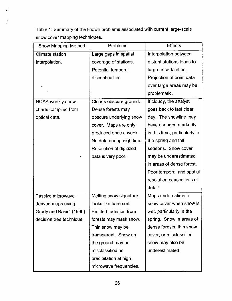
Table 1: Summary of the known problems associated with current large-scale

snow cover mapping techniques.

Snow Mapping Method Problems Effects

Climate station

interpolation.

NOAA weekly snow

charts compiled from

optical data.

Passive microwave-

derived maps using

Grody and Basist (1996)

decision tree technique,

Large gaps in spatial

coverage of stations.

Potential temporal

discontinuities.

Clouds obscure ground.

Dense forests may

obscure underlying snow

cover. Maps are only

produced once a week.

No data during nighttime.

Resolution of digitized

data is very poor.

Melting snow signature

looks like bare soil.

Emitted radiation from

forests may mask snow.

Thin snow may be

transparent. Snow on

the ground may be

misclassified as

precipitation at high

microwave frequencies.

Interpolation between

distant stations leads to

large uncertainties.

Projection of point data

over large areas may be

problematic.

If cloudy, the analyst

goes back to last clear

day. The snowline may

have changed markedly

in this time, particularly in

the spring and fall

seasons. Snow cover

may be underestimated

in areas of dense forest.

Poor temporal and spatial

resolution causes loss of

detail.

Maps underestimate

snow cover when snow is

wet, particularly in the

spring. Snow in areas of

dense forests, thin snow

cover, or misclassified

snow may also be

underestimated.

26

Table 2: SSM/I data record 1987-1995.

Days with no PM data

1987:340,347,354,361

1988: 3, 10, 129, 360

1989: 15, 204,295

1990: 238,294,301,315,

Days with no 85GHz

channel

1989:36 -365

1990:7- 364

Days when PM data

coverageis poor

1988:150,276,290,318,

332

1989:78

1990:49,322,336,364

357

1991:69

1992:159

1994: 170,310, 324

1991:6 - 335 1991:6,62,139,342

1992:33,348

1993:122

1994:37-121,317,359

1995:148

27

Table 3: Percent of climate stations reporting snow within each MDSCP snow-

cover class. The data are the mean values for the winter months (DJF) for the

period 1987through 1995.

MDSCP snow-cover

class

Thin or patchy snow

High elevation snow

Fully snow covered

Mean number of

stations in class

Mean percent

snow cover

1177

3O2

1549

34.3

24.6

75.4

Mean standard

deviation

5.85

6.37

3.73

28

I

I

I Does PM show snow?

I Is there a swath gap?

N Iy_ oo_,_soshowsnow_]

1YI Is the terrain complex? I

N

Are there at least 2

nearby climatestations?

N

1Is the terrain complex? I

N

I Are there at least2 Inearby climate

stations?Nl

Y =[ Are there at least2

I nearby climatestations?

_-I_ I Do all nearby stationsshow no snow?

r

--_/ Is the air temperature

/ less than 273K?

Are there at least 2

nearby climatestations?

._! Do at least 2 nearby / Nstations show no

snow? Y

[ Do at least2 nearby ]

I stations show no isnow?

N I

N

Y'-I Do at least 2 nearby

stations show nosnow?

Yl

Y

Y

"l Do at least 2 nearby _ Nstations show no /snow? y

J

_[ Does NSC show snow? _ Is the terrain/

Ncomplex? I

lN YIN

_N Does NSC show snow? I

Y

I Are there any nearby II Are there at least 2climate stations? 1t nearby climatestations?

lY IN _Y11

Do all nearby stations IIshow no snow? I1

Do at least 2 nearbystations show no

snow?

JY lN

_| Do at least 2 nearby

L stations show nosnow?

YY _[ Are there at least 2

/ nearby climatestations?

Nl

Are there at least 2 _ Do all nearby stations t-_ Do at least 2 nearbynearby climate show no snow? stations show no

stations? I 1 I t snow?

N[ IY IY

N

Y

High ElevationSnow Cover

I Is the terraln complex? ]

I41 Do all nearby stations

t show snow?

Y

J l Fully SnowCovered

I

Is the terrain complex? If

_.__[ Are there at least 2

nearby climatestations?

VNo Snow

Cover

N YI

Y

I

tThin or Patchy

Snow Cover

Y

a. b.

c. do

Fully snow-covered

No snow-cover

Air temperature <273K

D Thin or patchy snow

Sea-ice cover

Air temperature >273K

i_ High elevation snow

D PM swath gap

SATELLITE SNOW COVER14-18 Jan 1995

United States

N_ opm_eom] Hydrobgt¢Remote $mslng Cemcr

Oflke of Hydroloi_, National Weather _ NOAAlVflmNapelh,Minnesota

I SNOW

NO SNOW

CLOUD

MULTIPLE-DATASET

SNOW COVER PRODUCT15 Jan 1995

Snow

Pa_hy Snow

High El. Snow

No Snow

25 I I I I I I I

20-

(,0,,,,_

Eo

15-

0

Cr

o 10

C

.o

5t

0 I 1 I

1988 1989

I L_...... I

1990

I

I991

I I I I I

]..... I I I J

1992 199,.5

I I 1 .....

I-

I I L .____

1994 1995

40"l

Eo

5

i..,.

O

:Z$

O-09

o 203

C-

O

I 1 t I I I I I t I

0

A

L

/\

- i \

/ _ ,,.

I J: i I I I i • _l ..... __-

S 0 N D J F M A M d d

t/']

(D-.i-.,

1E0

@

07 0O-

S

c- -10

-2

-3

271

-IIIIIIIIIIIIIIIIIII111111111111

\ _ j r -- --

_ ,, /

". /\

--. /

/\ /_

k /\

7

J/

J

I I I I I I I 1 I • 1 I I_L I J I I I I 1 I _ l J.__l J I I I I

292 51,3 534 555 010 051 052 073 094 1 I5

Julian day

©

E0

00

ET"6"3

,4,-

0

03

[2

0

-1

-2

271

III1111111111111111111tlltlltlt

I I I I I I I I I I J I I I I I I I I I_ I_ ] _I I._I i

292 313 334 355 010 031 052 073 094 115

Julicn doy

03,,,__

E0

...,.

C)

Z3

0"-

O3

0

O3

C

0

15

10

5

1989

I I I I I I I I I I I I I

I I I I I

1990

I I I I 1 I

1991

I

1992