?r=19990064061 2018-01-22t18:55:46+00:00z · pdf fileas a contribution to ... human shelter,...

https://ntrs.nasa.gov/search.jsp?R=19990064061 2018-05-09T21:59:59+00:00Z

Front cover: Image of Western Hemisphere as taken by GOES 8 meteorological

satellite in September 1994.

Published by

National Aeronautics and Space Administration

as a contribution to

United Nations Office of Outer Space Affairs

for UNISPACE III

NOTE: This report has been produced without full editorial revision by NASA. The

designations employed and the presentation of the material in this publication are solely

those of the lead authors and does not imply endorsement by NASA of the ideas ex-

pressed.

Design and Production by: Michele Meyett (Center of Excellence in Space Data and

Information Sciences at NASA/GSFC)

NASA Scientific Forum

on Climate Variabilityand Global Change

20 July 1999

UNISPACE III

Robert A. Schiffer

Sushel Unninayar

THIRD UNITED NATIONS CONFERENCE

ON THE EXPLORATION AND PEACEFUL

USES OF OUTER SPACE

19 - 30 JULY 1999

Contents

Foreword

[Ghassem Asrar, Associate Admin, NASA] ....................................................................... iii

Ozone Depletion, UVB and Atmospheric Chemistry

[Richard Stolarski, NASA/GSFC] ....................................................................................... 1

Global Climate System Change and Observations

[Kevin Trenberth, NCAR] ................................................................................................. 15

Predicting Decade-to-Century Climate Change: Prospects for Improving Models

[Richard Somerville, SIO] ................................................................................................. 31

Sun-Climate Connections

[Judith Lean, NRL] ............................................................................................................ 43

Seasonal to Interannual Climate Variability and Predictability

[Jagadish Shukla, COLA] .................................................................................................. 59

El-Niho: Monitoring, Prediction, Applications, Impacts

[Chester Ropelewski & Dr. Antonio Moura, IRI] .............................................................. 71

Cooperation Between Space Agencies and the Worm Climate Programme (WCRP)

[Hartmut Grassl, WMO/WCRP] ........................................................................................ 79

Forum Program Plan: see inside back cover

Abbreviations

COLA ..................... Center for Ocean-Land-Atmosphere StudiesIRI .......................... International Reserach Institute for Climate Prediction

NASA/GSFC .......... National Aeronautics Space Administration/Goddard Space Flight CenterNCAR ..................... National Center for Atmospheric Research

NRL ........................ Naval Research LaboratorySIO .......................... Scripps Institution of OceanographyWMO/WCRP ......... World Meteorological Organization/World Climate Research Programme

Foreword

The Forum on Climate Variability and Global Change is intended to provide a glimpse

into some of the advances made in our understanding of key scientific and environmental

issues resulting primarily from improved observations and modeling on a global basis.

The climate of the Earth system is a consequence of a complex interplay of extemal solar

forcing and internal interactions among the atmosphere, the oceans, the land surface, the

biosphere and the cryosphere. Surface climate generally defines thresholds for the sus-

tainability of water resources, agriculture, human shelter, transportation and health among

others. Variability within the climate system has significant impact on natural and man-

aged resources on all space and time scales, posing a particularly acute challenge to better

observe the Earth system, understand interactive processes, and improve conceptual Earth

system models. Inter-annual variability in the coupled ocean-atmosphere system is best

exemplified by the well known EI-Nino/Southem Oscillation event and its counterpart

cold phase, the La-Nina; impacts are generally world wide. We now know that human

activities are increasingly recognized as a potential factor forcing change in the global sys-

tem by altering the chemical composition of the atmosphere and the oceans as well as the

character of the land surface and vegetation cover. Increasing atmospheric concentrations

of powerful greenhouse gases such as CO2 and CH4 are predicted to lead to accelerated

global climate change, a central environmental issue of concern to Governments around

the world. Of particular interest are the potential regional impacts of such changes on

coastal areas, fresh water resources, food production systems, and natural ecosystems.

Space-based technology has advanced to a point that we are able to accurately observe and

sense globally the entire Earth system and to understand Earth system processes that arecentral to Earth's climate. We need to document and understand the Sun-Earth connection

as an external forcing of the Earth's climate, and also need to better understand the Earth's

intricately linked internal processes such as the global water, energy and carbon cycles.

Space-based platforms with their unique capacity to observe the Earth on a global basis,

complement surface-based and in-situ measurements. Together with advances in comput-

ing and information system technology, modem data assimilation techniques, diagnostic

and prediction models, they provide a powerful combination of tools for understanding of

the Earth system and applying the knowledge and tools to the management of natural

resources and the mitigation of natural hazards.

NASA's Earth Science Enterprise (ESE) is dedicated to using this unique combination of

space-based information system technologies and scientific expertise to support the study

of the Earth system and its environment. Active and passive remote sensing systems span-

ning a wide range of spatial, spectral and temporal coverage will contribute to capturing

and documenting the state of the Earth's atmosphere, continents, oceans and life. The vari-

ety of high precision and well calibrated remotely sensed Earth observations that will be

obtained by these missions will be unprecedented. We view this as a U.S. contribution to

the international efforts to cooperatively develop a comprehensive international Earth

111

observing strategy to benefit humankind. The NASA Earth Observing System (EOS) is aprogram of multiple spacecraft (30 satellites to be launched into low Earth orbit between

1999 and 2005) and interdisciplinary science investigations to provide a 15-year data set

of key parameters/processes needed to gain a better understanding of global climate pro-

cesses. The first series of EOS satellite launches in 1999 include, Landsat-7, QuikScat,

and Terra missions that will comprehensively monitor the Earth system. Preceding EOS, a

number of individual satellite and the Space Shuttle-based missions are helping reveal the

basic processes of atmospheric chemistry (Upper Atmosphere Research Satellite-UARS/

1991), ozone distribution (Total Ozone Mapping Spectrometer-TOMS/1978, 1991, 1996,

and 2000), ocean topography and circulation (YOPEX/Poseidon/1992), ocean winds

(NASA Scatterometer-NSCAT/1996), ocean color (SeaWifs/1997), and global tropical

energy and precipitation (Tropical Rainfall Measuring Mission-YRMM/1997), among oth-

ers. These provide the scientific foundation on which EOS builds. For example, TRMM is

providing unprecedented data on energy and precipitation processes and distribution in the

tropics that will contribute substantially to the understanding of the global hydrological

cycle. Landsat-7 was successfully launched in 1999 to continue and improve the data

series provided by previous Landsat missions for 26 years since 1972. Later this year ESE

will conduct the Shuttle Radar Topography Mission to use interferometric synthetic aper-

ture radar to produce the first globally consistent and high precision digital-elevation

model. We also plan to launch the Active Cavity Radiometer Irradiance Monitor (ACRIM)

mission in 1999 to consolidate and extend over 20 years of observations of total solar irra-diance.

EOS-PM, to be launched in year 2000 will provide unprecedented capability to monitor

the Earth system, particularly: atmospheric temperature and humidity/water vapor pro-

files, radiation budget, clouds and aerosols, precipitation, sea surface winds, sea surface

temperature, ice, snow, soil moisture, ocean color/biomass, vegetation cover/land produc-

tivity, among others. The SeaWinds scatterometer on Japan's ADEOS II mission to con-

tinue the measurements of sea surface wind vectors, and the US/France Jason-l--a

follow-on to the highly successful TOPEX/Poseidon mission to capture sea surface topog-

raphy which is also an indicator of upper ocean heat content; both are scheduled to be

launched in the year 2000. In addition, we will launch the New Millennium Program Earth

Observer-1 technology demonstration mission, designed to make future Landsat-type mis-

sions possible at vastly reduced size and cost. The New Millennium Program provides for

the infusion of innovative new technologies with an initial focus on continuation of the

systematic measurements, and will emphasize fast-track development and low-cost dem-

onstration missions. These technologies, will lead to the development of smaller and

lighter-weight instruments in order to be responsive to new and emerging scientific chal-

lenges requiring space-based observations.

Complementing EOS will be a series of small, rapid-development Earth System Science

Pathfinder (ESSP) missions to study emerging science questions and make innovative

measurements in parallel with the 15-year mission of EOS. ESSP will feature low life-

cycle costs, and missions based on best science value. The first two ESSP missions, Vege-

tation Canopy Lidar (VCL), and Gravity Recovery and Climate Experiment (GRACE), a

joint endeavor with Germany, are scheduled for launch in 2000 and 2001, respectively.

iv

PICASSO-CENA, a joint endeavor with France, is planned to be launched in 2003 to

study for the first time the three dimensional structures of the atmosphere, in particular,

clouds, aerosols and volcanic plumes, and their role in the Earth's climate. CloudSat, a

joint effort with Canada, will be launched in 2003 to provide significantly better data on

vertical structure of thick clouds and their role in the Earth's radiation budget.

NASA's Earth Science Enterprise has adopted an evolutionary approach to fulfill its mis-

sions and goals. Future missions needed to achieve continuity for systematic measure-

ments, together with those in the exploratory mode of ESSP, will be implemented

according to the "better/faster/cheaper" paradigm. NASA will invest up-front in technol-

ogy development, and base its mission selection on both scientific need and technology

readiness. This will enable NASA to respond to emerging scientific observational needs

in a timely fashion. The goal is to develop and launch the next generation of Earth observ-

ing satellites in 2 to 3 years instead of 7 to 10 years which is normal practice today.

Overall, it is an exciting era for space-based Earth observing systems, with significant

research and operational applications benefits. With the advances being made in all coun-

tries, we hope to meet the needs for global Earth and environmental observations through

a coordinated, cooperative strategy, firmly based on our scientific understanding of cli-

mate variability, environmental and global change issues of importance to nations around

the world. The knowledge gained from these efforts will benefit equally natural resource

managers, city planners, cartographers, and policy makers. Earth is the only planet in the

solar system that supports carbon based life. Indeed it is the prime real estate of our solar

system to support the current and future generations. It is time for the nations around the

world to position themselves such that we benefit collectively from these wonderful tech-

nological innovations, and to foster establishment of sound environmental policy deci-

sions for management and preservation of the Earth's unique conditions.

Ghassem R. Asrar

Associate Administrator

Office of Earth Science

NASA Headquarters

Washington, D.C.

OzoneDepletion,UVBandAtmosphericChemistry[R.Stolarski]

OZONE DEPLETION, UVB AND ATMOSPHERIC CHEMISTRY

Richard S. Stolarski

NASA Goddard Space Flight Center

Laboratory for Atmospheres

([email protected])

Background

Chapman's Pure Oxygen Model

The primary constituents of the Earth's atmosphere are molecular nitrogen and molecular

oxygen. Ozone is created when ultraviolet light from the sun photodissociates molecular

oxygen into two oxygen atoms. The oxygen atoms undergo many collisions but eventu-

ally combine with a molecular oxygen to form ozone (03). The ozone molecules absorb

ultraviolet solar radiation, primarily in the wavelength region between 200 and 300

nanometers, resulting in the dissociation of ozone back into atomic oxygen and molecular

oxygen. The oxygen atom reattaches to an 02 molecule, reforming ozone which can then

absorb another ultraviolet photon. This sequence goes back and forth between atomic

oxygen and ozone, each time absorbing a uv photon, until the oxygen atom collides with

and ozone molecule to reform two oxygen molecules. This sequence can be summarized

by the following equations:

Production:

hv + O2---_ O+O

Cycling:

0+02+M---903+M

hv + 03 ---_, 02 + 0

Destruction:

0 + 03 ----> 02 + 02

This sequence of reactions is called the Chapman mechanism after Sidney Chapman who

first proposed it in 1930. At high altitudes, the concentration of 02 necessary for the pro-

duction of O and 03 decreases so that the concentration of ozone decreases with increas-

ing altitude. At lower altitudes the solar ultraviolet radiation responsible for the

production of ozone is absorbed by 02 and by 03 . Thus the concentration decreases with

decreasing altitude. This leads to a peak in the ozone at an altitude between these

extremes. This peak occurs in the stratosphere where the ozone reaches concentrations of

5-10 parts per million by volume (ppmv).


()zone Destruction by Catalysis

In the 1960s and early 1970s it was realized that the destruction reaction can be enhanced

by catalytic reactions involving the oxides of hydrogen, nitrogen, chlorine, and bromine.

For instance, chlorine atoms can act as a catalyst for ozone destruction through the simple

two-step sequence:

C1 + 0 3 ---_ C10 + 0 2

C10 + O --- _ C1 + 0 2

The net result of these two reactions is the recombination of an O and an 03 to reform to

02 molecules, exactly duplicating the destruction reaction in the Chapman mechanism.

The chlorine atom has survived the reactions to participate in further cycles. Similar

cycles occur with the chlorine atom replaced by NO, OH, or Br.

The existence of these catalytic compounds in the stratosphere depends on a source. The

compounds themselves, such as chlorine atoms, C10 molecules, NO molecules, etc. can-

not be readily transported from the ground to the stratosphere. During the slow journey of

ground-level air up into the stratosphere, the molecules undergo many reactions forming

compounds such as the acids HC1 and HNO 3. These are soluble in water and will be

removed during rain, adding to the acidity of that rain. Instead, unreactive and insoluble

forms of chlorine and nitrogen can carry these atoms into the stratosphere. Nitrous oxide

(laughing gas, N 20) is a product of the nitrogen cycle in soils. It is insoluble and unreac-

rive. Upon reaching the stratosphere it will react with excited oxygen atoms produced

during the photolysis of ozone. This reaction produces two nitric oxide (NO) molecules.

The primary source of chlorine in today's stratosphere is the photodissociation of industri-

ally-produced chlorotiuorocarbons (CFCs). These insoluble, unreactive compounds

include CFC-11 (CFC13) and CFC-12 (CF2C12). Because the time to transport these

sources of catalytic compounds to the stratosphere is long, small sources can lead to sig-

nificant accumulation over time. The reactions are catalytic and small amounts of cata-

lysts can affect much larger concentrations of ozone. Thus, parts per billion of the

catalysts can have a significant effect on the parts per million of ozone.

Meteorological Effects

The description of the photochemistry of stratospheric ozone given above does not explain

all of the observed features of the concentration of ozone in the atmosphere. The photo-

chemical theory would predict a peak in ozone at the equator where the solar radiation

received is a maximum. Observations show a minimum in the ozone amount at the equa-

tor and a seasonally-varying maximum at high latitudes. The high-latitude maximum

occurs in the spring and is located near the pole in the northern hemisphere and about 30

degrees off the pole in the southern hemisphere.


This lead Dobson and Brewer in the late 1940s to postulate a slow circulation in which ris-

ing air entered the stratosphere from below in the tropics and then proceeded poleward

and eventually downward at mid and high latitudes. Thus air enters the stratosphere in the

tropics with relatively low amounts of ozone characteristic of the troposphere. As that air

is lofted to higher altitudes and latitudes, ozone is created by the ultraviolet photodissocia-

tion of 0 2 in a region where the photochemistry is fast. This air is transported downward

and poleward where ozone accumulates. There, enough ozone accumulates that it absorbs

the ultraviolet radiation which leads to its own destruction. Ozone destruction slows

down in the lower stratosphere because little uv radiation is available to produce atomic

oxygen. The lifetime of ozone in the midlatitude lower stratosphere becomes as long as a

year or more.

The picture that we now have of stratospheric ozone is one of photochemical production

and loss plus dynamical redistribution of that ozone. The dynamical redistribution leads

to the springtime seasonal high latitude peaks in the ozone amount. It also leads to the

very different distribution of ozone in the southern and northern high latitudes. Dynami-

cal redistribution leads to daily variations in ozone as weather systems pass through the

midlatitudes. The total column amount of ozone exhibits time-varying patterns that look

very much like the weather maps seen on the television news.

Penetration of UV Radiation

One of the primary properties of ozone is its strong absorption of ultraviolet radiation.

The total column amount of ozone in the atmosphere is approximately 1019 molecules per

cm 2. At a wavelength of 250 rim, the ozone absorption cross section is 10 -17 cm 2. This

means that radiation of 250 nm from the sun will be absorbed such that its intensity is

reduced by e -l°° from that which impinges on the top of the atmosphere. Thus, no radia-

tion at wavelengths near 250 run reaches the ground.

Of more concern are the wavelengths near 300 nm. These wavelengths still possess

enough energy in a photon to break important bonds in biological molecules and their

cross sections are small enough that some of the radiation from the sun can reach the

ground. At 320 nm the cross section is about 2.5 x 10 -2°. Thus the radiation from the sun

is reduced by e-°.25 when the sun is overhead. When the sun is lower in the sky, the reduc-

tion in the radiation is greater because of the greater path length of ozone through which

the radiation must pass. When the column amount of ozone overhead varies, so too does

the amount of uv radiation at wavelengths near 300 nm which is received at the ground.

This radiation at the ground is affected by other factors. These include clouds, haze or

aerosols, and the reflectivity of the surface.

Ozone Depletion

Ozone depletion is usually defined as a change in ozone brought about by a change in the

chemicals which lead to ozone loss. This can be brought about either by direct injection or

Ozone Depletion, UVB and Atmospheric Chemistry [R. Stolarski]

by a change in the source gases. Thus there exists a "normal" amount of nitrogen oxides

in the stratosphere due to production from nitrous oxide as a part of the natural cycle of

nitrogen fixation and denitrification. This cycle can be changed by the addition of fertil-

izer nitrogen which enhances nitrogen cycling and produces more N20. A more direct

way to enhance stratospheric nitrogen oxides is the direct injection by aircraft flying in the

stratosphere.

A ircra_ Effects

Aircraft engines burn fuel at high temperatures (-3000°C). At these temperatures the

nitrogen and oxygen in the air passing through the engine are broken down and a portion

of nitrogen oxides are produced. The current fleet of subsonic aircraft fly in both the tro-

posphere and lowest part of the stratosphere. In this region, the primary effect of the

added NOx is the enhancement of the smog-like chemistry of the oxidation of methane.

The result is an enhancement of ozone. In the early 1970s, a great deal of research was

done on the possibility of a fleet of commercial supersonic transports which would fly in

the stratosphere near 20 km altitude. At 20 km altitude, the effectiveness of the smog

chemistry has decreased and the catalytic effects of the added nitrogen oxides begins to

dominate.

Over the last l0 years, the idea of a commercial fleet of supersonic planes, now called the

high-speed civil transport (HSCT) has been revived. Studies now reveal that reactions on

the background sulfate aerosols in the stratosphere affect the balance of the nitrogen and

chlorine chemistry. Thus added NOx increases the rate of ozone loss through the NOx cat-

alytic cycle. At the same time, added NOx ties up more chlorine as chlorine nitrate

(CIONO2) and decreases the rate of ozone loss through the chlorine cycle. The net effect

on ozone is a combination of the direct catalytic effect of NO x and of its interference with

the chlorine cycle. This leads to a calculated net ozone loss at 20 km from this hypotheti-

cal fleet which is small (fraction of a percent). One unsolved problem is the determination

of what fraction of the exhaust, from a fleet flying primarily at midlatitudes, would reach

the tropics and be lofted to higher altitudes where aerosol concentrations are small. A

small fraction of the exhaust reaching 30 km altitude could dominate the loss from the

NO x catalytic cycle.

Airplanes exhaust also contains water vapor and sulfur compounds. The water vapor

leads to an increase in atmospheric hydrogen oxides which catalytically destroy ozone.

Sulfur leads to the formation of small particles which increase the surface area of aerosols

in the stratosphere. Increased surface area converts more chlorine to the active form C10,

and thus increases the ozone loss due to chlorine catalytic cycles.

Chlorofluorocarbons

Chlorofluorocarbons are source gases for stratospheric chlorine. They are long-lived com-

pounds which are not reactive, nor soluble in water. The most common of the CFCs are

CFC-11 (CFC13) and CFC-12 (CF2C12). These, and numerous other CFCs, are industri-


ally-producedcompoundswhichdid notexist in theatmospherebeforetheir inventionin aDuPontlaboratoryby Midgley in the 1930s.

Despitetheir atomicweightsof approximately100,CFCsarethoroughlymixed through-out the troposphereby small-scalemotions,and arelofted to high altitudesby the slowtransportcirculationof theatmosphere.In thestratosphere,with muchof theozonelayerbelow them, CFCsaredestroyedby theabsorptionof uv photonswhich free a chlorineatomleavingafast-reactingfragment. Subsequentrapidchemistryreleasestherestof thefluorineandchlorineatomsfrom theCFCmolecule.

Productionof CFCsbeganin the 1930sand grew exponentiallyinto the 1970s. Theirgrowth becamean issuein themid 1970sandin 1977theUnited Statespasseda banontheir useasapropellantin aerosolspraycans. Figure1 illustratesthereleaseratefor onespecificchlorofluorocarbon,CFC-11. Thereleaserategrewrapidly until about1975whenit levelledoff andevendecreaseda little. Thenthereleaseratebeganto grow againuntilthe MontrealProtocolwasagreeduponin 1987. After that thereleaseratedeclinedrap-idly. The concentration of CFC-11 in the atmosphere responds only slowly to these

changes in the production rate. The residence time of CFC- 11 in the atmosphere is about

50 years. The loss rate is proportional to the amount in the atmosphere which continues to

increase even as the production rate is decreasing. Eventually the production rate

becomes small enough that the loss rate is greater and the concentration begins to

decrease. Figure 1 shows that we are about at that level in the late 1990s for CFC-11.

CF C-I 1 Production and Cont:_tratioa

40O

01940 1960 1910 2000

Ye/IF

Figure 1: Time history of the production rate of CFC-11 and its atmospheric concentration.

Production rate is given on the left scale while concentration in parts per trillion by volume

is given on the right scale.


Other chlorine containing compounds are at different stages in this evolution. The rate of

increase of the CFC-12 concentration has slowed but not ceased. The concentration of

methyl chloroform (CH3CCI3) in the atmosphere is clearly decreasing. The concentration

of some of the replacement HCFCs (e.g. HCFC-141b or CH3CC12F ) are increasing rap-

idly. The concentrations of all of these compounds can be taken together to indicate the

amount of chlorine which will be available to the stratosphere as a function of time. This

compilation shows that the available chlorine peaked in about 1994 and has decreased

slightly since that time. There is a time delay of about 5 years between the peak in chlo-

rine potentially available at the ground and chlorine available in the stratosphere. Thus,

the peak in stratospheric chlorine should be occurring about now.

Once the chlorine is freed from the CFCs by ultraviolet absorption in the stratosphere, itundergoes a set of reactions which convert it from one molecular form to another. These

reactions result in a quasi-steady-state in which the proportion of chlorine in each com-

pound is determined by local factors such as the amount of solar ultraviolet radiation, the

temperature, the concentration of ozone, and the concentration of other radicals such as

OH and NO 2. In the midlatitude lower stratosphere, where the ozone concentration is a

maximum, most of the chlorine available is converted into the temporary reservoir mole-

cules HCI and CIONO 2. This is accomplished via the reactions:

CI + CH 4 ' _ HCI + CH 3

C10 + NO 2 + M -- _ C1ONO 2 + M

Chlorine is returned to the catalytically active C1/CIO cycle by the reactions:

. __ -_

HC1 + OH C1 + H20.___

CIONO 2 + hv CIO + NO 2

These reactions come to a balance in which a relatively small fraction of the chlorine is in

the catalytically active C1 and CIO.

Thus, CFCs carry chlorine to the stratosphere. Once there, the chlorine begins to catalyti-

cally destroy ozone. The chlorine is converted to reservoir molecules such as HC1 and

C1ONO 2. The reservoirs are converted back to active chlorine which continues to destroy

ozone. This continues during the entire time that the chlorine is in the stratosphere. The

chlorine is eventually transported out of the stratosphere on the downward-moving branch

of the circulation at midlatitudes. During its residence time in the stratosphere, a typical

chlorine atom can destroy as many as 104 to 105 molecules of ozone.

Bromine and halons

Bromine is an even more effective catalyst for ozone loss than is chlorine. Bromine mon-

oxide (BrO) can react with itself to reform bromine atoms or it can react with C10 to

reform bromine and chlorine atoms. This generates a catalytic cycle which does not need


atomic oxygenfor its completion. Sinceatomicoxygenis in shortsupply in the lowerstratosphere,thesebrominecyclesaremuchmoreeffectivetherethanthecyclesrequiringatomicoxygen.

Bromineis suppliedto theatmospheremainly asmethyl bromide(CH3Br). Methyl bro-mide hasbothnaturalandanthropogenicsources. It arisesnaturally from oceanswherebromineatomsreplaceiodinein methyl iodideproducedby seaweed.It is alsodestroyedin oceanswherechlorineatomscandisplacethebromine,forming methyl chloride. There

is also a major anthropogenic source of CH3Br. It is used as a fumigant for crops like

strawberries. A field is covered with a plastic and CH3Br is injected underneath this cover

to kill the various pests which can ruin the fruit. The plastic is removed and the crops are

grown. Inevitably a fraction of this CH3Br is not destroyed during this process and is

released to the atmosphere. Uncertainties remain in the quantitative effect of anthropo-

genic bromine on the bromine budget of the stratosphere.

Other important sources of bromine to the stratosphere are the halons, particularly halon-

1211 (CBrCIF2) and halon 1301 (CBrF3). The concentration of these compounds is only a

few parts per trillion, but the rate of increase of all of the halons together is a little over

2%/year.

The Ozone Hole

By the early 1980s, predictions had been made of ozone changes which should occur dueto enhanced ozone loss from reactions of chlorine from CFCs. These changes were pre-

dicted to occur in the upper stratosphere and have a relatively small effect on the total col-

umn amount of ozone. The predicted effect was small enough that it could not have been

deduced from the data available. In 1985, Farman and colleagues published a paper on

their data taken from the Antarctic station at Halley Bay beginning in 1957. They found

that the average amount of ozone in the month of October had decreased from about 300

Dobson units (DU) to 180 DU. This observation was quickly confirmed using data from

the Total Ozone Mapping Spectrometer (TOMS) and Solar Backscatter Ultraviolet

(SBUV) instruments on the Nimbus 7 satellite. These instruments provided maps of the

entire Antarctic region which showed that the springtime ozone loss was occurring over an

area larger than the continent. It was clear that something was going on over Antarctica

that was very different from what was occurring over the rest of the globe.

The difference at high latitudes is the formation of the winter polar vortices. Strong west

to east winds circulate around the pole with a maximum velocity about 20 to 40 degrees

off of the pole. The circulation is such that little exchange of air takes place between the

polar region and the midlatitudes during the winter. This isolated pole is in the dark

through most of the winter. The air radiates to space and cools to temperatures low

enough that polar stratospheric clouds form despite the extremely dry nature of the strato-

sphere. The southern hemisphere polar region becomes more isolated and cold than does

the northern hemisphere polar region. The distribution of mountains and land masses in

the northern hemisphere causes the upward propagation of waves which distort and erode

the northern hemisphere vortex causing it to weaken and disappear before the spring in

most years.


Ozene < 2_0 DU O_W_> 4110DU

Antar_ic Ozone

5 October 1987

Figure 2: Schematic showing the extent of the ozone hole region for October 5, 1987. The

area where ozone is less than 220 DU is shaded. Also in lighter shading is the area where theozone amount is greater than 400 DU.

Air containing CFCs is well mixed in the troposphere. It enters the stratosphere in the

tropics and is spread toward the poles. Air finally reaching the poles has been in the

stratosphere an average of more than 5 years and has had much of its CFCs converted into

active or reservoir chlorine. In the polar night reactions occur on the surfaces of polar

stratospheric cloud particles which convert chlorine from the reservoir form to chlorine

gas C12. The most important of these reactions is:

HCI + C1ONO 2 --- -_ HNO 3 + CI 2

The nitric acid sticks to the particle and the CI 2 comes off as a gas. When the air sees sun-

light in the early spring, C12 is rapidly photodissociated to CI atoms which react with

ozone to form C10. C10 reacts with itself to form a dimmer Cl202 which absorbs sunlight

and photodissociates to C1 atoms and CIOO. These reactions form a catalytic cycle which


destroysozone without the use of atomic oxygen. The result is a rapid springtime

decrease in the ozone concentration of the lower stratosphere. This decrease is particu-

larly pronounced in the southern hemisphere where a minimum is reached during October.

Figure 3 shows the October monthly mean ozone amounts each year beginning in the late

1950s. During the 1950s, 1960s, and early 1970s, the October mean ozone amount over

the Halley Bay Station on the Antarctic continent was about 300 DU. This decreased

throughout the 1980s until the typical October mean amount was barely over 100 DU.

This situation has continued throughout the 1990s.

October Monthly Mean Omane

1001960 1970 1980 1990

Year

Figure 3: October monthly mean ozone amounts over Antarctica. The filled circles are the

monthly mean amounts measured over the Halley Bay Station by the Dobson instrument

located there (data courtesy J. Shanklin, British Antarctic Survey). The triangles are the

minimum monthly mean from the TOMS maps of total ozone over the Antarctic. The dia-monds are the similar data from the Nimbus 4 BUV instrument.

Another measure of the Antarctic ozone hole is its size. We saw in figure 2 an example of

a day when the region of ozone amounts less than 220 DU was larger than the size of the

continent of Antarctica. Figure 4 shows the average size of the ozone hole, as measured

by the various TOMS instruments, for each year since 1979. The size is defined as the

area where the ozone amount is less than 220 DU averaged between September 7 andOctober 13.

9


Measurementsby balloon-bornesondesindicatethat the ozoneloss is occurring in thelower stratospherebetweenabout 12and22km altitude. This is the regionof themaxi-mum in the ozoneconcentration. In recentyearsthe losshasbecomenearly completeover this regionandtheminimumamountof totalcolumneozonemeasuredis just that ataltitudesaboveandbelow theprimary depletionregion. Thus,theminimumamountsoftotalozonereachedin Octoberasshownin Figure3havenot continuedto declineasthereis nomoreozoneto be lostunlessthedepletionextendsto eitherhigheror lower altitudesthanbefore.

Long-term Global Trends

The Antarctic ozone hole provides the most spectacular example of changes in strato-

spheric ozone. Changes of a much smaller magnitude are also evident over large portions

of the globe. The deduction of long-term trends must be made by accounting for various

known natural variations of ozone. Ozone amounts vary on a seasonal cycle. At midlati-

tudes, this seasonal cycle is the dominant variation seen in the data. When an average sea-

sonal cycle is removed from the data, other variations become apparent. These include the

11-year solar cycle and the 27 month quasi-biennial oscillation (QBO). Finally, if all of

these variations are removed, the residual should show the trend, if any. Typically, these

analyses are done by fitting to a statistical model which contains terms for all of the varia-

tions including the trend and the residual noise.

Ave__e Area of Ozone Hole30, , , ,, , ,, ,, , , ,, ,, , , , , ,,I I

]

V

01980 1985 3990 1995

YGal"

Figure 4: Area of Antarctic ozone hole as defined by ozone amounts less than 220 DU. Filled

circles indicate the area averaged from September 7 to October 13 of each year. Verticalbars indicate the daily range of the area over this time period.

10


Theresultingtrendsfrom onesuchcalculationareshownin Figure5 asa functionof lati-

tude and season. Small, insignificant trends are deduced for the equatorial region. Trends

in the southern hemisphere springtime are large as the region of the Antarctic ozone hole

is approached. Northern hemispheric trends show a strong seasonal variation with a max-

imum negative trend in the winter and early spring.

TOMS V7 Total Ozone TrendNov 78-Apr 93 (%IDecade)

60

4O

_I 20"ID

•_ 0|m

cg--I-2o

-4O

--60

J F M A 1.1 J J A S 0 14 D

Month

Figure 5: Trends in total ozone deduced from the data ofthe Nimbus 7 TOMS instrument for

the time period from late 1978 through May of 1993.

Prospects for recovery

We saw above that the provisions of the Montreal Protocol have already resulted in a

marked decrease in the production of some important CFCs. At the same time, production

of replacement compounds has increased. The total amount of tropospheric organic chlo-

rine compounds determines the amount of chlorine which is available for transport to the

stratosphere. The sum of the chlorine in these compounds was determined to have peaked

sometime in 1994. About a 5-year delay is expected before that turnaround would be seen

in stratospheric chlorine available for ozone depletion. Satellite measurements of the res-

ervoir gas, HCI indicate that a leveling off in the available chlorine is beginning to take

place in the stratosphere. Thus, the driving term for stratospheric ozone loss should be

now leveling off.

11


How soonwill it bebeforewecanseetheresultin theozone data itself?. The time varia-

tions of the CFCs and of HCI were dominated by the trend term. It was thus relatively

easy to observe the flattening out of these time series. The same is not true of ozone. Its

variations are dominated by natural causes and the trend terms are not dominant.

One method for testing for early evidence of a flattening out of the trend was used recently

by Lane Bishop in the recent UNEP/WMO Ozone Assessment Report. He used the glo-

bally-integrated ozone amount because that record averages out much of the strong sea-

sonal and interannual variation. He then fit the data from 1979 through mid 1991 (pre-

Pinatubo) to a standard statistical model with terms for seasonal variation, trend, QBO,

solar cycle, and noise. That calculation is reproduced below in Figure 6 for the TOMS

data from three satellites; Nimbus 7, Meteor 3, and Earth Probe.

Figure 6 shows only two terms from the statistical model fit; the annual mean trend term

and the residual noise. Put another way, Figure 6 shows the data minus the model fit for

the annual cycle, the solar cycle, the QBO, and the annual component of the trend term.

The upper panel shows the data in the same form as analyzed by Bishop, using the calibra-

tions given with each satellite data set. The lower panel shows the same calculation using

satellite data which has been renormalized to the overpasses of the ground-based network

of ozone-measuring stations.

The top panel of Figure 6 shows the Earth Probe TOMS data from 1996-1998 to be well

above the extrapolated trend line (-2%). This would provide some indication of the

beginning of recovery except for the uncertainty in the establishment of the Earth Probe

TOMS calibration with respect to the calibration of the Nimbus 7 and Meteor 3 TOMS

instruments. It is also worth noting that the estimated uncertainty on global trends is

greater than 1%/decade (2_) which would place the Earth Probe data on the edge of sig-nificance even if the calibration were to be believed.

The bottom panel, where the ground-based adjustment has been used, shows the recent

Earth Probe TOMS data to be only marginally above the extrapolated trend line. This is

well within the uncertainty of the determination of that trend line. This data set thus pro-

vides no indication yet of any recovery. Note that the trend deduced from this data is

smaller than that deduced from the unadjusted TOMS data in the upper panel (-1.7%/

decade vs. 2.0%/decade).

We are currently working on producing an internally-consistent satellite data set which is

independent of the ground based network. This relies on using the data from the NOAA-9SBUV/2 to establish the relative calibration of Earth Probe and the other TOMS instru-

ments. This has proved difficult because of the drift in the orbit of NOAA-9.

UVB Radiation

There is a large and growing literature on the effects of UVB radiation and on the mea-

surement of the amount reaching the ground. Here we will only be able to make a briefstatement of some of the main issues.

12

Ozone Depletion, UVB and Atmospheric Chemistry JR. Stolarski]

TOMS MOD_VO -Seas -Solar -QBO -Seas Trend

0

i1980 1985 1990 1995

Year

TOMS MOD_V2b -Seas -Solar -QBO -Seas Trend

0

i1980 1985 1990 1995

Year

Figure 6: TOMS global average total ozone data. Shown is the residual from a statistical

model fit which includes seasonal variation, an ll-year solar cycle, a quasi-biennial oscilla-

tion, and a seasonal trend term. The residual is the annual mean trend plus the noise term.

The top panel shows data from three TOMS instruments using their original calibrations.

The bottom panel shows the same data using calibrations that have been adjusted by a

smoothed time-dependent offset determined from overpasses of a set of 38 ground-based sta-tions.

13


UVB is defined as the radiation between wavelengths of 285 nm and 315 nm. UVB radia-

tion at 285 nm is strongly absorbed by ozone while that at 315 nm is much more weakly

absorbed by ozone. Thus, more radiation at 315 nm penetrates the ozone layer than doesradiation at 285.

The UVB radiation which reaches the surface is affected by many factors in addition to

ozone absorption. Rayleigh scattering by atmospheric molecules reduces the amount of

direct-beam UVB but increases the diffuse component of UVB. Aerosols and haze cause

scattering which adds to the diffuse component of the UVB. Clouds affect UVB by both

reflection and scattering. Finally, surface reflectivity affects the UVB received near the

surface. For instance, snow or water surfaces increases the UVB dosage which leads to

sunburn.

Determination of the trend in UVB requires an absolute calibration in a given wavelength

region which must be maintained to high precision over a long period of time. UVB at the

surface is highly variable, both because ozone is variable and because of the cloudiness

and haze factors described above. In general, the best way to determine a trend in UVB

would be to measure it relative to some other wavelength of UV which is not expected to

show a trend in time. In fact, this is how ozone is measured; by the ratio of UVB to UVA

(_. > 320 nm). These measurements show a clear decrease in UVB relative to UVA.

With the provisions of the Montreal Protocol, we hope to be able to observe the slow

decrease in the net amount of UVB reaching the ground over the coming decades as the

ozone layer slowly recovers with the decrease in the atmosphere's chlorine content.

14

GlobalClimateSystemChangeandObservations[K.Trenberth]

GLOBAL CLIMATE SYSTEM CHANGE AND OBSERVATIONS

Kevin E. Trenberth

National Center for Atmospheric Research

sponsored by the National Science Foundation

([email protected])

,/'7

Abstract

Following a brief introduction to the climate system, a discussion is given of the natural

greenhouse effect and the enhancements arising from human activities and other agents of

change. The atmosphere is the most volatile component of the climate system and large

weather variability confounds the detection of small climate signals. The ocean is also

fluid and plays an active role. The atmosphere and oceans together can give rise to phe-

nomena that would not occur without interactions between them, with the best example

being E1-Nifio. Feedback processes are briefly discussed, including the critical role of

clouds. Observations of global climate change are summarized along with the need to be

able to assemble all the understanding into global climate models, which can then be used

to make better sense of the observations and to carry out numerical experiments. The

important role of changes in the hydrological cycle as well as temperatures is emphasized.

Even for instrumental observations, the long time-series of high quality observations

needed to discern small changes are often compromised by non-physical effects, and spe-

cial care is required in interpretation. From space, similar problems arise from the orbital

decay and drift in equator crossing times of individual satellites, the finite life time of

instruments and satellites which result in different platforms for instrtunents (even if the

same) and electronic noise from nearby instruments, calibration of instruments, and con-

version of radiances into geophysically meaningful quantities. Yet both systems have sub-

stantial advantages. A call is made for a true sustained climate observing system

composed of both space-based and in situ components that capitalizes on the advantages

of each.

The Climate System

The internal interactive components in the climate system include the atmosphere, the

oceans, sea ice, the land, snow cover, land ice, and fresh water reservoirs (Figure 1). The

greatest variations in the composition of the atmosphere involve water in various phases in

the atmosphere, as water vapor, clouds of liquid water, ice crystal clouds, and hail. How-

ever, other constituents of the atmosphere and the oceans can also change and humans are

having a discernible influence, so this brings considerations of atmospheric chemistry,

marine biogeochemistry, and land surface exchanges into climate change. The main focus

in this article is on the atmosphere as the most variable component of the Earth system; it

is afterall where we live and makes up the air we breathe.

15

Global Climate System Change and Observations [K. Trenberth]

o

!

B

o _

et i_

16

GlobalClimateSystemChangeandObservations[K.Trenberthl

The source of energy which drives the climate is the "short wave" radiation from the sun

and much of this energy is in the visible. Because of the roughly spherical shape of the

Earth, at any one time half the Earth is in night and the average amount of energy incident

on a level surface outside the atmosphere is one quarter of the total solar irradiance or 342

Wm -2. About 31% of this energy is scattered or reflected back to space by molecules, tiny

airborne particles (known as aerosols) and clouds in the atmosphere, or by the Earth's sur-

face, which leaves about 240 Wm -2 on average to warm the Earth's surface and atmo-

sphere (Figure 2), see Kiehl and Trenberth (1997) for details.

To balance the incoming energy, the Earth itself must radiate on average the same amount

of energy back to space (Figure 2). It does this by emitting thermal "long-wave" radiation

in the infrared part of the spectrum. For a completely absorbing surface to emit 240

Wm -2 of thermal radiation, it would have a temperature of about -19°C. This is much

colder than the conditions that actually exist near the Earth's surface where the annual

average global mean temperature is about 15°C. However, because the temperature in the

troposphere falls off quite rapidly with height, a temperature of-19°C is reached typically

at an altitude of 5 km above the surface in mid-latitudes. This provides a clue about the

role of the atmosphere in making the surface climate hospitable.

The Greenhouse Effect

Some of the infrared radiation leaving the atmosphere originates near the Earth's surface

and is transmitted relatively unimpeded through the atmosphere; this is the radiation from

areas where there is no cloud and which is present in the part of the spectrum known as the

atmospheric "window". The bulk of the radiation, however, is intercepted and re-emitted

both up and down. The emissions to space occur either from the tops of clouds at different

atmospheric levels (which are almost always colder than the surface), or by gases present

in the atmosphere which absorb and emit infrared radiation. Most of the atmosphere con-

sists of nitrogen and oxygen (99% of dry air) which are transparent to infrared radiation.

It is the water vapor, which varies in amount from 0 to about 3%, carbon dioxide and some

other minor gases present in the atmosphere in much smaller quantities which absorb

some of the thermal radiation leaving the surface and re-emit radiation from much higher

and colder levels out to space. These radiatively active gases are known as greenhouse

gases because they act as a partial blanket for the thermal radiation from the surface and

enable it to be substantially warmer than it would otherwise be, analogous to the effects of

a greenhouse. This blanketing is known as the natural greenhouse effect. In the current

climate, water vapor is estimated to account for about 60% of the greenhouse effect, car-

bon dioxide 26%, ozone 8% and other gases 6% for clear skies (Kiehl and Trenberth

1997).

Agents of Change and Feedbacks

The Earth System can be altered by effects or influences from outside the planet usually

17


regarded as "externally" imposed. Most important are the sun and its output, the Earth's

rotation rate, sun-Earth geometry and the slowly changing orbit, the physical make up of

the Earth system such as the distribution of land and ocean, the geographic features on the

land, the ocean bottom topography and basin configurations, and the mass and basic com-

position of the atmosphere and ocean. These components determine the mean climate

which may vary from natural causes. A change in the average net radiation at the top of

the atmosphere due to perturbations in the incident solar radiation or the emergent infrared

radiation leads to a change in heating. Changes in the net incident radiation energy at the

Earth's surface might occur from the changes internal to the sun but may also occur from

changes in atmospheric composition such as may arise from natural events like volcanoes,

which can create a cloud of debris that blocks the sun. Other forcings that might be

regarded as external include those arising as a result of human activities.

Evidence for human influences are all around. Most obvious are the changes in land use

and building cities. Conversion of forest to cropland, in particular, has led to a higher

albedo in places such as the eastern and central United States and changes in evapotranspi-

ration, both of which have probably cooled the region, in summer by perhaps I°C and

especially in autumn by more than 2°C, although global effects are less clear (Bonan

1997). In addition, storage and use of water (dams, reservoirs, irrigation) is important.

While there is substantial generation of heat by human activities for space heating, gener-

ation of electricity and so on, the amounts are small compared with the through/tows from

natural systems. Locally, in cities, these effects are important and combine to produce the

"urban heat island". However, the process of generating some of the heat through com-

bustion of fossil fuels also generates particulate pollution, (e.g., soot, smoke) as well as

gaseous pollution that can become particulates (e.g. sulfur dioxide, nitrogen dioxide;

which get oxidized to form sulfate and nitrate particles), and carbon dioxide. Human

activities also generate other gases: methane, nitrous oxide, the chlorofluorocarbons

(CFCs) and tropospheric ozone (especially from biomass burning, landfills, rice paddies,

agriculture, animal husbandry, fossil fuel use, leaky fuel lines, and industry). The result is

changes the composition of the atmosphere.

Moreover, the gases mentioned are all greenhouse gases and thus are radiatively active in

perturbing the heat flows on Earth, and many also have long lifetimes. The average life-

time of carbon dioxide is estimated to be over 100 years before it is taken out of the sys-

tem. Consequently, continual emissions of these gases lead to increased concentrations

which are clearly evident from measurements. Carbon dioxide has increased by over 30%

over the past 200 years, and mostly after World War II. Atmospheric aerosols also change

the composition of the atmosphere but typically have a lifetime of only a week or less

mainly because they are washed out by precipitation processes. Consequently aerosols are

mainly found relatively close to their sources and predominantly in the Northern Hemi-

sphere or tropics (the latter from biomass burning), whereas the greenhouse gases become

globally distributed and result in global forcings of climate.

18


19


Increased heating leads naturally to expectations for increases in global mean tempera-

tures (often mistakenly thought of as "global warming"), but other changes in weather are

also important. Increases in greenhouse gases in the atmosphere produce global warming

through an increase in downwelling infrared radiation, and thus not only increase surface

temperatures but also enhance the hydrological cycle as much of the heating at the surface

goes into evaporating surface moisture. Global temperature increases signify that the

water-holding capacity of the atmosphere increases and, together with enhanced evapora-

tion, this means that the actual atmospheric moisture increases, as is observed to be hap-

pening in many places (Trenberth 1998, 1989). It follows that naturally-occurring

droughts are likely to be exacerbated by enhanced drying. Thus droughts, such as those

set up by EI-Nifio, are likely to set in quicker, plants will wilt sooner, and the droughts

may become more extensive and last longer with global warming. Once the land is dry

then all the solar radiation goes into raising temperature, bringing on the sweltering heatwaves.

Further, globally there must be an increase in precipitation to balance the enhanced evapo-

ration. The presence of increased moisture in the atmosphere implies stronger moisture

flow converging into all precipitating weather systems, whether they are thunderstorms, or

extratropical rain or snow storms. This leads to the expectation of enhanced rainfall or

snowfall events, which is also observed to be happening (Karl and Knight 1998, Trenberth

1998), see Figure 3.

The response of the climate system to the agents of change is complicated by feedbacks in

the climate system, some of which amplify the original perturbation (positive feedback)

and some of which diminish it (negative feedback). If, for instance, the amount of carbon

dioxide in the atmosphere were suddenly doubled, but with other things remaining the

same, the outgoing long-wave radiation would be reduced by about 4 Wm -2 and instead

trapped in the atmosphere. To restore the radiative balance, the atmosphere must warm up

and, in the absence of other changes, the warming at the surface and throughout the tropo-

sphere would be about 1.2°C. In reality, many other factors will change, and various feed-

backs come into play, so that the best estimate of the average global warming for doubled

carbon dioxide is 2.5oC (IPCC, 1990, 1995). In other words the net effect of the feed-

backs is positive and roughly doubles the response otherwise expected.

The main positive feedback comes from water vapor as the amount of water vapor in the

atmosphere increases as the Earth warms and, because water vapor is an important green-

house gas, it amplifies the warming. However, increases in cloud may act either to

amplify the warming through the greenhouse effect of clouds or reduce it by the increase

in albedo; which effect dominates depends on the height and type of clouds and varies

greatly with geographic location and time of year. Ice-albedo feedback probably leads to

amplification of temperature changes in high latitudes. It arises because decreases in sea

ice and snow cover, which have high albedo, decrease the radiation reflected back to space

and thus produces warming which may further decrease the sea-ice and snow cover extent.

However, increased open water may lead to more evaporation and atmospheric water

vapor, thereby increasing fog and low cloud amount, offsetting the change in surfacealbedo.

2o


Figure 3: Schematic outline of the sequence of processes involved in climate change and how

they alter moisture content of the atmosphere, evaporation, and precipitation rates. All pre-

cipitating systems feed on the available moisture leading to increases in precipitation rates

and feedbacks. From Trenberth (1999).

21


Other more complicated feedbacks may involve the atmosphere and ocean, and the main

example is the set of processes that give rise to the EI-Nifio-Southern Oscillation (ENSO)

phenomenon in the tropical Pacific Ocean. The surface winds drive the ocean currents and

patterns of upwelling, determine the sea surface temperatures, which in turn determine the

preferred locations of atmospheric convection and tropical rainfall. These dominate the

tropical atmospheric heating and thus determine the local and even global atmospheric cir-

culation, through teleconnections, which include the surface winds. As this system is per-

turbed it sets up a positive feedback loop as an E1-Nifio or La Nifia event, and certain

negative feedbacks, including slow ocean adjustments to atmospheric effects from a year

or two previously, and changes in heat content within the ocean lead to the demise of the

events. Another example is the cold waters offofthe western coasts of continents (such as

California or Peru) that encourage development of extensive low stratocumulus cloud

decks which block the sun and this helps keep the ocean cold. A warming of the waters,

such as during EI-Nifio, eliminates the cloud deck and leads to further sea surface warm-

ing through solar radiation. Warming of the oceans from increased carbon dioxide may

diminish the ability of the oceans to continue to take up carbon dioxide, thereby enhancing

the rate of change, as more remains in the atmosphere.

A number of feedbacks involve the biosphere and are especially important when consider-

ing details of the carbon cycle and the impacts of climate change. For example, in wetland

soils rich in organic matter, such as peat, the presence of water limits oxygen access and

creates anaerobic microbial decay which releases methane into the atmosphere. If climate

change acts to dry the soils, aerobic microbial activity develops and produces enhanced

rates of decay which releases large amounts of carbon dioxide into the atmosphere.

Much remains to be learned about these feedbacks and their possible influences on predic-

tions of future carbon dioxide concentrations and climate. Adequate observations to better

understand these processes are needed as well as the ability to observe changes in the rele-vant variables to allow these effects to be determined.

Observed Climate Change

Analysis of observations of surface temperature show that there has been a global mean

warming of about 0.7oC over the past one hundred years; see Figure 4 for the instrumental

record of global mean temperatures. The warming became noticeable from the 1920s to

the 1940s, leveled off from the 1950s to the 1970s and took off again in the late 1970s.

The warmest year on record, by far, is 1998. The previous record was for 1997. The last

ten years are the warmest decade on record. Moreover, recent information from paleodata

further indicates that these years are the warmest in at least the past 1,000 years, which is

as far back as a near-global estimate of temperatures can be made (Mann et al. 1998,

1999). The melting of glaciers over most of the world and rising sea level confirms the

reality of the global temperature increases. The observed trend for a larger increase in

minimum than maximum temperatures is linked to associated increases in low cloud

amount and aerosol as well as the enhanced greenhouse effect (Dai et al. 1999).

22


There is firm evidence that moisture in the atmosphere is increasing. In the Western Hemi-

sphere north of the equator, annual mean precipitable water amounts below 500 mb are

increasing over the United States, Caribbean and the North Pacific by about 5% per

decade as a statistically significant trend from 1973 to 1993 (Ross and Elliott 1996), and

these correspond to significant increases in relative humidities of 2 to 3% per decade over

the Southeast, Caribbean and subtropical Pacific. Precipitable water and relative humidi-

ties are not increasing significantly over much of Canada, however, and are decreasing

slightly in some areas. In China, recent analysis by Zhai and Eskridge (1997) also reveals

upward trends in precipitable water in all seasons and for the annual mean from 1970 to

1990. A claim for recent drying in the tropics by Schroeder and McGuirk (1998) using

TOVS data is questionable owing to the changes in instruments and satellites. Clearly,

there is a need to obtain more reliable atmospheric moisture trends over the entire globe.

Moreover, there is clear evidence that rainfall rates have changed in the United States.

This has been shown by an analysis of the percentage of the U.S. area with much above

normal proportion of total annual precipitation from 1 day extreme events, where the latter

are defined to be more than 2 inches (50.8 mm) amounts (Karl et al. 1996). The "much

above normal proportion" is defined to be the upper 10%. This quantity can be reliably

calculated from 1910, and the percentage has increased steadily from less than 9 to over

11%, a 20% change. Karl and Knight (1998) have provided further analysis of U.S. pre-

cipitation increases and show how it occurs mostly in the upper tenth percentile of the dis-

tribution and that the portion of total precipitation derived from extreme and heavy events

is increasing at the expense of more moderate events. Other evidence for increasing pre-

cipitation rates occurs in Japan and Australia.

Anmml Global Surfso_ TemlPe_ure Ahomales0.8-

I_1_ porl_l 1961-1_

0,6-

0.4-

0.2-

oC0-

-0.2-

-0.4-

-1

0

-0.8-1850 18_0 1900 Ig20 1940 IOBO 19110 20DI)

Year

Figure 4: Global annual mean temperatures from 1860 to 1998 as departures from the 1961

to 1990 means. (Courtesy Jim Hurrell, adapted from data provided by Hadley Center,

UKMO, and Climate Research Unit, Univ. East Anglia).

o F

-4

23


Modeling the Climate System

A full climate system model should deal with all the physical, chemical and biological

processes that occur in nature and the interactions among the components of the climate

system, the atmosphere, ocean, land surface, sea ice, surface hydrology, and biosphere

(Figure 1). The models and their components are based upon physical laws represented by

mathematical equations which are solved using a three dimensional grid over the globe. A

major component of climate models are so-called atmospheric general circulation models

(AGCMs) which are designed to simulate the detailed evolution of weather systems and

weather phenomena, as well as the physical and dynamical processes involved. For

AGCMs, typical resolutions for climate simulations are about 250 km (156 miles) in thehorizontal direction and 1 km in the vertical.

It is well established that there is a limit to the predictability of weather of about two

weeks owing to the mathematical phenomenon now known as "chaos" in which small

uncertainties in the analysis of current weather conditions rapidly grow and eventually

become large enough to render the forecast worthless. This essentially random error com-

ponent is overcome in climate forecasts by predicting only the statistics of the weather,

i.e., the climate. Accordingly, systematic influences of changing conditions in the ocean,

sea ice, land surface, solar radiation, or other factors are reflected in atmospheric varia-

tions on various time scales. The most obvious example is the climate change with theseasons.

Climate models can be used in four-dimensional data assimilation (4DDA) to produce

global analyses of variables in a multivariate analysis that uses the model to help define

inter-relationships in a physically and dynamically consistent way. Once the models have

been adequately tested and validated (see Trenberth 1997), they can be used in numerical

experiments to make projections of possible future outcomes or to determine the climate

response to various forcings.

An ensemble of several climatic simulations, each of which begins from somewhat differ-

ent starting conditions, can be used to clearly establish which climatic features are repro-ducible in the simulations and thus are predictable with the model. These features

constitute the "climate signal", while those which are not reproducible can be considered

weather-related "climate noise". Climate predictability is a function of spatial scales.

Natural atmospheric variability is enormous on small scales and most climate forcings,

such as from increases in greenhouse gases, are predominantly global. Hence the noise

level of natural variability will increasingly mask a climate signal as smaller regions are

considered. Production of multiple repetitions of each experiment with small variationsrequires enormous computer resources.

Top-of-the-atmosphere Radiation and Clouds

Clouds absorb and emit thermal radiation and have a blanketing effect similar to that of

the greenhouse gases. But clouds are also bright reflectors of solar radiation and thus also

24


act to cool the surface. Consequently,the effectsof clouds can be clearly seen on the

Absorbed Solar Radiation (ASR) and the Outgoing Longwave Radiation (OLR)(Figure 5).

However, on average there is strong cancellation between the two opposing effects of

short-wave and long-wave cloud heating (Figure 5), and the net global effect of clouds in

our current climate, as determined by space-based measurements, is a small cooling of the

surface. A key issue is how clouds will change as climate changes. This issue is compli-

cated by the fact that clouds are also strongly influenced by particulate pollution, which

tends to make more smaller cloud droplets, and thus makes clouds brighter and more

reflective of solar radiation. These effects may also influence precipitation. If cloud tops

get higher, the radiation to space from clouds is at a colder temperature and so this pro-

duces a warming. If low clouds become more extensive, then this is more likely to pro-

duce cooling because of the greater influence on solar radiation. Observational evidence

indicates that increases in cloud amounts have been occurring (Dai et al. 1999).

The geometry of the Earth-sun system and the orbit of the Earth around the sun largely

determines the distribution of net radiation, although with important structure associated

with clouds, as noted above. However, the equator-to-pole and land-sea differences that

exist drive atmospheric and oceanic circulations that transport moisture, heat and energy

around the globe. Overall, the vertically-integrated divergence of the total atmospheric

transport of energy, which consists of dry static energy, latent energy and kinetic energy, is

balanced by the net radiative flux through the top of the atmosphere plus the flow into the

oceans. In turn, the latter is balanced by the redistribution of heat within the oceans by

ocean currents. Any small imbalances contribute to such things as changes in temperature.

With the observations in Figure 5, and others from space and from the ground, we are able

to compute the heat, moisture and energy budgets in detail and provide more and more

information on the workings of our climate system, improve models, and increase the

challenges for improved and new observations.

Observing the Earth and Monitoring Climate Change

We usually view the climate system from our perspective as individuals on the surface of

the Earth. Just a few decades ago, the only way a global perspective could be obtained

was by collecting observations of the atmosphere and the Earth's surface made at points

over the globe and analyzing them to form maps of various fields, such as temperatures.

The observational coverage has increased over time, but even today is not truly global

because of the sparse observations over the southern oceans and the polar regions. Earth

observing satellites have changed this, as two polar-orbiting sun-synchronous satellites

can provide global coverage in about 6 hours, and geostationary satellites provide images

of huge portions of the Earth almost continuously. However, it is difficult to see below

the ocean surface, and observations in the ocean domain remain few and far between.

2_


E_4

¢

x05

ED6

BD_,

E_E:EA_:_u,dNeun1t_15U_bmxl_d SDlar _:41=l_n TN

QatlPDUR IrI_DM _kO I_D 34{I BY Sn

-_._.,_=II I-

Znrml Mmmm

,.I .I I.

\

//

III'I I"

_IIrGUR rRDM Idl_ Ta II| BY 2|

1"m II B_ I _ _ I I

\/_L

Figure 5: Net, ASR and OLR annual means from the Earth Radiation Budget Experiment(ERBE) based on the period February 1985 to April 1989, as reprocessed by Trenberth

(1997b).

26


Even for instrumental observations, the long time-series of high quality observations

needed to discern small changes are often compromised by non-physical effects, and spe-

cial care is required in interpretation. Most observations have been made for other pur-

poses, such as weather forecasting, and therefore typically suffer from changes in

instrumentation, instrument exposure, measurement techniques, station location and

observation times, and in the general environment (such as the building of a city around

the measurement location) and there have been major changes in distribution and numbers

of observations. Adjustments must be devised to take into account all these influences in

estimating the real changes that have occurred.

From space, similar problems arise from the orbital decay and drift in equator crossing

times of individual satellites, the finite life time of instruments and satellites which result

in different platforms for instruments (even if the same) and electronic noise from nearby

instruments, calibration of instruments, and conversion of radiances into geophysically

meaningful quantities.

We need to know how the climate has changed and is changing. And because the future

climate will be different from that today, we need to develop the capability to make reli-

able predictions of what it will be. Such predictions start from the initial observed state:

not just for the atmosphere as in weather forecasting, but also for the oceans and every

other active component of the climate system. In future, routine observations from a vari-

ety of networks could provide a much more comprehensive snapshot of the state of the

environment: from space, from autonomous profiling floats at various depths the ocean,

and from new sensors. The challenge is to ensure that we have in place a means not only

to measure these variables, but to do so in a manner that enables us to understand whether

multi-decadal observed changes reflect real changes in the environment versus different

methods of observing.

In order to reduce our uncertainty about the sensitivity of the climate system to human

alteration of the environment, it will be critical to evaluate our model simulations. We

must be capable of adequately simulating the climate during pre-industrial times, and

especially since that time, when humans have changed the composition of the atmosphere

in a dramatic manner. To evaluate our models we require not only snapshot pictures of

many physical, chemical, and biological quantities, but reliable long-term records. How-

ever, we are dependent on services of large operational networks that are presently being

operated for purposes other than studying climate change. We currently do not have an

adequate system for monitoring climate.

In addition to the standard atmospheric variables (temperatures, winds) much better fields

are needed for clouds, water vapor and ozone, and probably other trace constituents, as

well as precipitation. At the surface, surface winds (from scatterometry) and sea level

(from altimetry), ocean color, soil moisture, as well as glacial ice volume will be impor-

tant. Also important will be continuing measurements of any forcings of climate, such as

the total solar irradiance, and the four dimensional distribution of aerosol loading from

volcano and human sources and top-of-the-atmosphere radiation. Many of these fields can

be obtained from space but information, such as vertical structure, is also needed from the

27


ground,andmeasurementswithin theoceanmustcomefrom in situ sources.Synthesisofall the measurementsandgenerationof importantproductsmustcomefrom globalmod-els,andfour-dimensionalassimilationmustplaya majorrole.

In the past,space-basedsystemsmeasurementshavebeenconvertedto geophysicalvari-ablesusingvariousalgorithms.Increasingly,4DDA makesdirectuseof radiancesalongwith informationon all othervariablesin amultivariateanalysis.A new challenge,there-fore, is to determinewhat arethe requirementsfor radiancesthat shouldbemeasuredtoproducetherequiredaccuracyof geophysicalvariables?A relatedchallengeis to includebiascorrectionsfor variousobservingsystems(satelliteandin situ) asthey changewithtime.

A call is madefor a trueclimate observingsystemcomposedof bothspace-basedandinsitu componentsthat capitalizeson the advantagesof eachandwhich adheresto guidingprinciples that ensurelong term integrity. The space-basedcomponentproducesregularglobal coveragebut is not stable. Multiple overlappingsatellitescanhelp transfertherecord from one satellite to another,but all satellitessuffer from orbital decayand driftthat alter the time of day of measurements.While advancedstation-keepingcanhelp,thereis alsoaneedfor astableground-basedclimateobservingsystem.Thein situ instru-mentscanbe changedas long as overlapsare includedas part of the strategyand thespace-basedrecordcanalsohelptransfertherecordacrosstransitions. Methodsof moni-toring observingsystemperformanceand processingall the datawith appropriatebiascorrectionsmust alsobea part of this. Specialeffortsandinstitutionalcommitmentsareneededto designandsustainsuchasystem.

References

Bonan,G. B. (1997). Effectsof landuseontheclimateof theUnitedStates.Clim.

Change, 37, 449-486.

Dai, A., Trenberth, K. E. and Karl, T. R. (1999). Effects of clouds, soil moisture, precipi-

tation and water vapor on diurnal temperature range. J. Clim., (in press).

Houghton, J. T., Meira Filho, F. G., Callander, B. A., Harris, N., Kattenberg, A. and

Maskell, K. (Eds.). (1996). IPCC (Intergovernmental Panel of Climate Change). Cli-

mate Change 1995." The Science of Climate Change. (pp. 572) Cambridge, U.K.: Cam-

bridge Univ. Press.

Karl, T. R., and Knight, R. W. (1998). Secular trends of precipitation amount, frequency

and intensity in the USA. Bull. Am. Meteorol. Soc., 79, 231-242.

Karl, T. R., Knight, R. W., Easterling, D. R. and Quayle, R. G. (1996). Indices of climate

change for the United States. Bull. Am. Meteorol. Soc., 77, 279-292.

28


Karl, T. R.,Knight, R. W.andPlummer,N. (1995). Trendsin high frequencyclimatevariability in thetwentiethcentury.Nature, 377, 217-220.

Kiehl, J. T., and Trenberth, K. E. (1997). Earth's annual global mean energy budget. Bull.

Am. Meteorol. Soc., 78, 197-208.

Mann, M. E., Bradley, R. S. and Hughes, M. K. (1998). Global-scale temperature pat-

terns and climate forcing over the past 6 centuries. Nature, 392, 779-787.

Mann, M. E., Bradley, R. S. and Hughes, M. K. (1999). Northern hemisphere tempera-

tures during the past millennium: Inferences, uncertainties, and limitations. Geophys. Res.

Lett., 26, (in press).

Ross, R. J., and Elliot, W. P. (1996). Tropospheric water vapor climatology and trends

over North America: 1973-93. J. Clim., 9, 3561-3574.

Schroeder, S. R., and McGuirk, J. P. (1998). Widespread tropical atmospheric drying

from 1979 to 1995. Geophys. Res. Lett., 25, 1301-1304.

Trenberth, K. E. (1997). The use and abuse of climate models in climate change research.

Nature, 386, 131-133.

Trenberth, K. E. (1997b). Using atmospheric budgets as a constraint on surface fluxes. J.

Climate, 10, 2796-2809.

Trenberth, K. E. (1998) Atmospheric moisture residence times and cycling: Implications

for rainfall rates with climate change. Clim. Change, 39, 667-694.

Trenberth, K. E. (1999) Conceptual framework for changes of extremes of the hydrolog-

ical cycle with climate change. Clim. Change, 40, (in press).

Zhai, E, and Eskridge, R.E. (1997). Atmospheric water vapor over China. J. Clim., 10,

2643 -2652.

29

Predicting Decade-to-Century Climate Change: Prospects for Improving Models [R. Somerville]

PREDICTING DECADE-TO-CENTURY CLIMATE CHANGE:

PROSPECTS FOR IMPROVING MODELS

Richard C. J. Somerville f " _':"_" 7/

University of California, San Diego

Scripps Institution of Oceanography

([email protected])

Abstract

Recent research has led to a greatly increased understanding of the uncertainties in today's

climate models. In attempting to predict the climate of the 21st century, we must confront

not only computer limitations on the affordable resolution of global models, but also a

lack of physical realism in attempting to model key processes. Until we are able to incor-

porate adequate treatments of critical elements of the entire biogeophysical climate sys-

tem, our models will remain subject to these uncertainties, and our scenarios of future

climate change, both anthropogenic and natural, will not fully meet the requirements of

either policymakers or the public. The areas of most-needed model improvements are

thought to include air-sea exchanges, land surface processes, ice and snow physics, hydro-

logic cycle elements, and especially the role of aerosols and cloud-radiation interactions.

Of these areas, cloud-radiation interactions are known to be responsible for much of the

inter-model differences in sensitivity to greenhouse gases. Recently, we have diagnosti-

cally evaluated several current and proposed model cloud-radiation treatments against

extensive field observations. Satellite remote sensing provides an indispensable compo-

nent of the observational resources. Cloud-radiation parameterizations display a strong

sensitivity to vertical resolution, and we find that vertical resolutions typically used in glo-

bal models are far from convergence. We also find that newly developed advanced param-

eterization schemes with explicit cloud water budgets and interactive cloud radiative

properties are potentially capable of matching observational data closely. However, it is

difficult to evaluate the realism of model-produced fields of cloud extinction, cloud emit-

tance, cloud liquid water content and effective cloud droplet radius until high-quality mea-

surements of these quantities become more widely available. Thus, further progress will

require a combination of theoretical and modeling research, together with intensified

emphasis on both in situ and space-based remote sensing observations.

Introduction

Seen from space, the Earth appears as a mainly blue ocean planet flecked with constantly

changing intricate patterns of white clouds. The clouds, which cover about half the sur-

face of the planet, are critical to climate. They cool the Earth by reflecting away sunlight.

At the same time, they warm the Earth by trapping the Earth's heat, thus contributing to

the natural greenhouse effect. Of course, clouds are also a source of water in the form of

31


rain and snow, critical to all aspects of life and central to agriculture and thus to the well-

being of humankind. If climate changes, whether for natural or man-made reasons, clouds

are likely to change as well and have important feedbacks on the climate.

In computer modeling of the global climate system, which is our main technique for fore-

casting future climate, we first have to understand climate science well enough to build

crucial physical processes into our models realistically. Among the key science areas,

treating clouds accurately is an especially critical issue, because clouds have such impor-

tant effects on climate. However, clouds are much too small and short-lived to be mod-

eled explicitly in a global simulation, and the physical processes involved in clouds are

still imperfectly understood. Nevertheless, clouds and their consequences are much too

important to be ignored, and so their effects are treated by simple rules.

Climate models are solved numerically on global grids with a typical resolution of a few

hundred kilometers horizontally. When the model values of climate variables at this reso-

lution are used to prescribe clouds, the resulting rules are often highly simplistic. For

example, a typical rule might make the cloud amount in a model grid area proportional to

relative humidity. However, the behavior of rules of this sort often bears little resem-

blance to the way clouds actually vary in space and time in the present atmosphere, let

alone as to how they will change and feed back on any future climate which differs from

the present one. These rules are rarely well-founded theoretically and have almost never

been tested observationally in any thorough and satisfying way.

It is crucial that observational and modeling research be done to show how clouds behave

in the actual atmosphere. Only recently have appropriate observations begun to be avail-

able to tackle this task. These observations provide invaluable information for the devel-

opment of improved models. Space-based data have been critical to progress. Supporting

the research to obtain and use these data optimally is a key to further progress in making

future climate projections reliable, detailed and useful to policymakers.

Research strategy

Progress in attacking these questions depends on a multi-faceted research strategy. It is

now well-recognized in the community that single-column models (SCMs) are tools

which have a valuable role to play in testing and improving parameterizations by evaluat-

ing them empirically against field observations. E. g., see Randall et al. (1996). This

paper features some representative examples of the ability of SCMs to aid in evaluating

and improving global climate model (GCM) parameterizations.

Our SCM contains switch-selectable parameterizations based on current GCM practice.

Our approach involves evaluating parameterizations directly against measurements from

field programs, and using this validation to tune existing parameterizations and to guide

the development of new ones. We use the single-column model (SCM) to make the link

between observations and parameterizations. Surface and satellite measurements are both

used to provide an initial evaluation of the performance of the different parameterizations.

The results of this evaluation are then used to develop improved cloud-precipitation

schemes, and finally these schemes are tested in GCM experiments (Lee et al., 1997).

32

PredictingDecade-to-CenturyClimateChange:ProspectsforImprovingModels[R.Somerville]

Our single-columnmodelhasevolvedfrom the one described by Iacobellis and Somer-

ville (1991a,b). The SCM now is a versatile and economical one-dimensional model,

resembling a single column of a general circulation model (GCM). The SCM contains the

full set of parameterizations of subgrid physical processes that are normally found in a

modem GCM. The SCM is applied at a specific site having a horizontal extent typical of a

GCM grid cell. Since the model is one-dimensional, the advective terms in the budget

equations are specified from observations. For a more complete discussion of SCMs, see

Randall et al. (1996) and Iacobellis and Somerville (1991a,b).

The standard SCM uses the longwave radiation parameterization of Morcrette (1990) and

the solar radiation parameterization of Fouquart and Bonnel (1980). A variety of parame-

terizations representing cumulus convection, cloud prognostication, cloud radiative prop-

erties, cloud water budgets and precipitation can be tested in this manner and used for

intercomparison. The cumulus convection parameterizations which we have used include

those of Kuo (1974) (as modified by Anthes, 1977) and of Arakawa and Schubert (1974)

(with downdrafts as specified by Kao and Ogura, 1987), and of Emanuel (1991). The

cloud prediction schemes are those of Slingo (1987), Smith (1990), Sundqvist et al. (1989)

and Tiedtke (1993). The cloud radiative properties are specified from either McFarlane et

al. (1992) or a combination of Stephens (1977) (water clouds) and Suzuki et al. (1993) (ice

clouds). Cloud liquid water is a prognostic model variable when the Smith or Sundqvist or

Tiedtke scheme is active, but not when the Slingo routine is being used. These parameter-

izations are switch-selectable in the present version of the model.

Model experiments

Long-term experiments in the TOGA-COARE region

As an example of the use of single-column models, we first present a series of seven

"long-term" experiments from the 1992-93 tropical field experiment TOGA-COARE

(Tropical Ocean Global Atmosphere - Combined Ocean-Atmosphere Response Experi-

ment). The model configuration in each experiment differs only in the specification of the

cumulus convection parameterization, the cloud prognostication scheme and/or the

parameterization of cloud-radiative properties. The parameterizations used in each experi-ment are shown in Table 1.

In each experiment, the SCM was applied at 19 5°x 5 ° sites within the bounded region of

the western tropical Pacific extending from 137.5°E-172.5°E and 7.5°N-7.5°S. The size

and location of the individual sites was selected to coincide with the ECMWF Operational

Analysis data which is used as model forcing in these experiments. Each experiment

extends from 01 November 1992 to 28 February 1993 which corresponds to the IOP ofTOGA-COARE. At each site the model was initialized at 01 Nov 1992 00LST and run for

a period of four days. The model was then reinitialized and run again for the next four

days. This process was repeated a total of 30 times with the last 4-day run extending from

25 February 1993 to 28 February 1993. These 30 runs were repeated at each of the 19 5°x

5 ° sites. Long-term regional means during the TOGA-COARE lOP are formed by averag-

33


ing resultsfrom the 570(19sitesx 304-dayperiods)modelrunsfor eachconfigurationofmodelparameterizations.

Table 1: Model Configurations

Exp. Cumulus Cloud Cloud-Radiative

No. Convection Scheme Properties

1 Kuo-Anthes Slingo McFarlane

2 Emanuel Slingo McFarlane

3 Arakawa-Schubert Slingo McFarlane

4 Kuo-Anthes Smith Stephens+Suzuki

5 Emanuel Smith Stephens+Suzuki

6 Arakawa-Schubert Smith Stephens+Suzuki

7 Kuo-Anthes Sundqvist Stephens+Suzuki

The cloud radiative forcing terms (Ramanathan et al. 1989; Senior and Mitchell, 1993)

and other cloud-radiation variables produced by the these SCM experiments can be exam-

ined to understand how the various parameterizations may affect the modeled climatolog-

ical heat budget of the TOGA-COARE region. The cloud radiative forcing represents the

extra amount of radiation that is either emitted to space or absorbed by the earth-atmo-

sphere system due to the presence of clouds. The total cloud forcing (CF) is composed of a

shortwave component (SWCF) and a longwave component (LWCF), or, in equation form:

CF = CFsw + CFLw = (Q- Qc) - (F- Fe)

where Q is the net incoming solar radiation, F is the outgoing longwave radiation and the

subscript c indicates clear-sky fluxes. If CF is positive then the clouds have a warming

effect on the earth-atmosphere system. These terms averaged over all 19 sites and over the

4 month time period for each of the seven SCM experiments are shown in Table 2. The

last row of Table 2 contains the observed values obtained from GMS-4 satellite measure-

ments (Flament and Bernstein, 1993).

These results show that when the Slingo cloud scheme is used (experiments 1-3) model

averages of CFsw, CFLw, OLR, albedo and insolation are less sensitive to the choice of

cumulus parameterization than when the Smith cloud scheme is employed (experiments 4-

6). The effect of the treatment of cloud liquid water can be seen by comparing the results

from experiments 1, 4 and 7. Here the Kuo-Anthes convection was used in each case

while the cloud prognostication scheme varied. The model results show large decreases in

insolation and OLR and large increases (in magnitude) in albedo and both the shortwave

and longwave cloud forcing terms for experiments 4 and 7 compared to experiment 1.

34


Table 2: Cloud Forcing and Radiative Results

Exp. CFsw CFL w CF Albedo OLR Insol.

No. (W m -2) (Wm -2) (W m -2) (W m -2) (Wm -2)

I -I00 56 -44 0.33 236 200

2 -101 57 -44 0.33 229 199

3 -108 65 -43 0.35 224 191

4 -121 66 -55 0.38 225 176

5 -137 76 -61 0.42 210 159

6 -144 82 -62 0.44 207 151

7 -138 71 -67 0.42 220 154

GMS -108 62 -46 0.37 228 ---

The model results are much closer to the observed GMS-4 values when cloud liquid water

is not an interactive variable (experiments 1-3). The larger absolute values of the cloud

forcing terms, the increase in albedo, and the decrease in OLR and insolation in experi-

ments 4-7, all indicate that the model is either over-estimating the cloud fraction and/or

the cloud optical thickness when cloud liquid water is an interactive variable.

Short-term experiments in the IFA region

The SCM is now applied over the site of the Intensive Flux Array (IFA). In this series of

experiments the horizontal advection terms necessary to force the SCM are derived from

sounding measurements taken along the perimeter of the IFA. Thus, direct observations

are used to force the model in these experiments as opposed to model assimilation prod-

ucts used in Section 3.1. The SCM was run for several 5-day periods within the TOGA-

COARE lOP of 0 INov92 - 28Feb93 using model configuration #7 (see Table 1).

Figure 1 shows results that typify the SCM response during low precipitation conditions

over the IFA. During these 'dry' events, the SCM typically reproduced the observed tem-

perature and humidity evolution and produced diagnostic radiative quantities that com-

pared very well to both surface and satellite measurements. SCM results from a 5-day

period that experienced significant precipitation are shown in Figure 2. During these 'wet'

events the SCM often underestimated the surface downwelling solar radiation and overes-

timated the planetary albedo while reproducing well the precipitation as measured by the

satellite measurements of the Microwave Sounding Unit (MSU).

35


296

o...294

292

_ 29O

288

TEMPERATURE (850MB)

--Model

.... Observed

300 DOWNWELLING

260

220

_: 1so

140

100

NOV 13 NOV 14 NOV lS NOV 16 NOV 17

Date (1992)

SURFACE SHORTWAVE

15AoQ

913

m 11

" 9tJ

e_u_

SPECIFIC HUMIDITY (850 MB)

430

420

e.

_410

t_

400

--Model

NOV 13 NOV 14 NOV 15 NOV 16 NOV 17

Date (1992)

DOWNWELLING SURFACE LONGWAVE

--Model

....Observed - Surface Sites

--Model

---Observed - Surface Sites 390

Daily Means 24-hr Running Means' ' 38(] , ,NOV 13 NOV 14 NOV 15 NOV 16 NOV 17 NOV 13 NOV 14 NOV lS

Date (1992) Date 11992)

iNOV 16 NOV 17

Figure 1: Model vs. observation comparisons for low-precipitation conditions

These model results from the IFA site are consistent with the long-term runs discussed

above in that they both indicate the model parameterizations are over-estimating the

cloudiness and/or cloud optical thickness. Further analysis of the model results indicates

that very large errors in cloud optical thickness would be necessary solely to explain themodel discrepancies in albedo and surface shortwave. Thus, overestimation of the frac-

tional cloud coverage is more likely to be the cause of the majority of the errors in albedo

and surface shortwave. The fractional cloud cover for convective clouds in the Sundqvist

cloud scheme is given by:

CLD = _x( 1 + RH)(1 + (a b - t_t)/A)/( 1 + B_x)

where CLD is fractional cloud amount, RH is relative humidity, fib, t_t are the sigma level

of cloud base and cloud top, g is a quantity proportional to the moisture convergence, x is

a convective time scale and A, B are constants. In Sundqvist's scheme, the values of A and

B are set to 0.3 and 2.5 respectively. We performed numerous SCM runs in the IFA region

throughout the lOP period, each run with different values of A and B. A comparison of

model albedo and surface shortwave to observations yielded "optimized" values of A and

B of approximately 0.5 and 4.0.

36


3OO

. 250

-_ 200

150

100

0.8

0.6

ea

__ 0.4<

0.2

0.0

DOWNWELLING SURFACE SHORTWAVE

--Model

..... Observed - Surface Sites

Daily MeansJ i _ J

FEB 03 FEB 04 FEB 05 FEB 06 FEB 07

Date (1993)

ALBEDO

Daily Means

--Model

-- Observed (GMS-4)


Date (1993)

BRIGHTNESS TEMPERATURE300_

2s0F _ ,_, / _-""

t \/_. 2so_ --Model

.ot230124-hr Runnin 8 Means _ _ ,

10.0


Date (19931

PRECIPITATION

8.0

6.0

o

.._ 4.0

"_,

2.0¢h

o.o

• Daily Means

--Model

.... Observed (MSU)

i i iFEB 03 FEB 04 FEB 0S FEB 06 FEB 07

Date (1993)

Figure 2: Model vs. observation comparisons for significant precipitation conditions

The use of these optimized values of A and B improves the SCM estimates of albedo and

downwelling shortwave radiation during precipitation events in the IFA region. A further

and more substantial test of this optimization was performed by rerunning the long-term

runs (SCM in configuration 7) with the optimized values of A and B. The model results

from the "optimized" run and the original run are shown below in Table 3, along withmeasured values from the GMS-4 satellite. The results from the SCM run using the opti-

mized values of A and B show a clear improvement over the original run when compared

to GMS-4 measurements taken during the TOGA-COARE IOP.

Table 3: Original vs. Optimized

CFsw CFLw CF Albedo OLR Insol.

(W m -2) (W m -2) (W m -2) (W m -2) (W m -2)

Original - 138 71 -67 0.42 220 154

Optimized - 112 59 -53 0.36 232 183

GMS -108 62 -46 0.37 228 ---

31


Summary and outlook

The results of global climate models (GCMs) are sensitive to small-scale physical pro-

cesses. Yet these processes are often treated simplistically and even crudely. For example,

we have considered in particular the task of treating the role of clouds in affecting radia-

tion, both solar and terrestrial, passing through the atmosphere. One needed quantity is

the cloud amount, i. e., the fraction of a GCM grid area covered by cloud at different alti-

tudes. Numerous observational studies demonstrate that cloud amount is not a simple

function of relative humidity.

Today, GCM parameterizations are held to a higher standard than only a few years ago,

because it has become recognized that the role of cloud feedbacks is crucial in determin-

ing the sensitivity of GCM climates to changes in the atmospheric concentration of carbon

dioxide and other greenhouse gases, and to the direct and indirect effects of atmospheric

aerosols. Early GCMs had fixed clouds and hence a low sensitivity to prescribed carbon

dioxide changes. When cloud amounts are parameterized on relative humidity, several

positive feedbacks come into play. One is the reduction of cloud amount in a warmer cli-

mate, a typical GCM result. This change produces an augmented warming, because GCM

clouds, like global average real clouds, have a larger contribution to the planetary albedo

than to the planetary greenhouse effect. In more precise terms, their shortwave forcing

dominates their longwave forcing.

A separate class of positive feedbacks arises from an increase in average cloud altitude,

which is also a characteristic GCM response to climatic warming. On average, higher

clouds are less effective infrared emitters to space, because they are colder, and they are

less effective reflectors of incoming solar photons, because they are optically thinner, than

lower clouds. In combination with the reduction in cloud amount, the increase in cloud

height has the effect of powerfully reinforcing the warming which gives rise to these

changes in cloud amount. It is the GCMs which incorporate these effects most strongly,

and which do not include compensating negative feedbacks, that produce the highest sen-

sitivities to changes in greenhouse gas concentrations.

The GCMs which have the lowest sensitivities, on the other hand, are those which are

dominated by negative cloud feedbacks. One such feedback is due to hypothetical cloud

microphysical processes. Chief among these is a hypothesized increase in cloud water

content accompanying a warmer climate. If in fact a warmer climate is characterized by

wetter clouds, then, other things being equal, the wetter clouds may produce a negative

feedback by increasing the optical thickness and hence the albedo of lower clouds, or a

positive feedback by increasing the infrared emissivity of optically thin higher clouds.

Which of these conflicting effects will dominate? Is it scientifically justifiable to focus on

global average cloud feedbacks to the neglect of regional ones? How do these cloud feed-

backs depend on season, or synoptic regime, or geographical locale? What are the dynam-

ical and thermodynamic consequences of the diabatic processes which depend on cloud

feedbacks. These questions form much of the research agenda of the climate community.

Even if anthropogenic climate change were not such an important policy issue, cloud pro-

38


cesses would play an important role in climate modeling, because they have such a perva-

sive influence on climate, as evidenced by recent GCM results (e. g., Lubin et al., 1998).

In this work, we have diagnostically evaluated several current and proposed model cloud-

radiation treatments against extensive field observations. Satellite remote sensing pro-

vides an indispensable component of the observational resources. We find that newly

developed advanced parameterization schemes with explicit cloud water budgets and

interactive cloud radiative properties are potentially capable of matching observational

data closely. However, it is difficult to evaluate the realism of model-produced fields of

cloud extinction, cloud emittance, cloud liquid water content and effective cloud droplet

radius until high-quality measurements of these quantities become more widely available.

Thus, further progress will require a combination of theoretical and modeling research,

together with emphasis on both in situ and space-based remote sensing observations.

We may draw several far-reaching conclusions from current climate research results:

. Predicting the future of Earth's climate, which can change for both natural and

human-related reasons, requires an improved understanding of key physical pro-

cesses, such as those related to clouds. Satellite measurements have been essential

to progress.

. The research needed to achieve this understanding is now underway, and the

needed measurements are beginning to be made, but much more effort is needed to

make key observations and use them to improve computer simulations. Space-

based measurements will continue to have a key role to play.

. Even after the research has been advanced and the models have become more

trustworthy, producing climate predictions with sufficient realism for policymak-

ers will require vastly increased computer power, and continuing scientific and

political leadership.

Acknowledgments

The research reported in this paper has been sponsored in part by the U. S. Department of

Energy under Grant DE-FG03-90-ER61061, the National Science Foundation under Grant

ATM91-14109, and the National Oceanic and Atmospheric Administration under Grant

NA36GP0372, and the National Aeronautics and Space Administration under Grant No.

NAG5-2238. I deeply appreciate the many essential contributions of my collaborators:

Carolyn Baxter, Joannes Berque, Sam Iacobellis, Dana Lane, Wan-Ho Lee and Boris

Shkoller.

39


References

Anthes, R.A. (1977). A cumulus parameterization scheme utilizing a one-dimensional

cloud model. Mon. Wea. Rev., 105, 270-286.

Arakawa, A., and Schubert, W. H. (1974). Interaction of a cumulus cloud ensemble with

the large-scale environment, Part I. J. Atmos. Sci., 31,674-701.

Bower, K. N., Choularton, T. W., Latham, J., Nelson, J., Baker, M. B. and Jenson, J.

(1994). A parameterization of warm clouds for use in atmospheric general circulation

models. J. Atmos. Sci., 51, 2722-2732.

Emanuel, K.A. (1991). A scheme for representing cumulus convection in large-scale

models. J. Atmos. Sci., 48, 2313-2335.

Flament, E and Bernstein, R. (1993). Images from the GMS-4 satellite during TOGA-

COARE (November 1992 to February 1993). (Technical report 93-06, 20pp, School of

Ocean and Earth Science and Technology). University of Hawaii, Honolulu (with two

CD-ROMs)

Fouquart, Y. and Bonnel, B. (1980). Computation of solar heating of the Earth's atmo-

sphere: a new parameterization. Beitr. Phys. Atmos., 53, 35-62.

Iacobellis, S. F., and Somerville, R. C. J. (1991a). Diagnostic modeling of the Indian

monsoon onset, I: Model description and validation. J. Atmos. Sci., 48, 1948-1959.

Iacobellis, S. F., and Somerville, R. C. J. (1991b). Diagnostic modeling of the Indian

monsoon onset, II: Budget and sensitivity studies. J. Atmos. Sci., 48, 1960-1971.

Kao, J. C.-Y. and Ogura, Y. (1987). Response of cumulus clouds to large-scale forcing

using the Arakawa-Schubert Cumulus Parameterization. J. Atmos. Sci., 44, 2437-2458.

Kuo, H. L. (1974). Further studies of the parameterization of the influence of cumulus

convection on large-scale flow. J. Atmos. Sci., 31, 1232-1240.

Lee, W.-H., Iacobellis, S. F. and Somerville, R. C. J. (1997). Cloud radiation forcings and

feedbacks: General circulation model tests and observational validation. J. Climate, 10,2479-2496.

Lubin, D., Chen, B., Bromwich, D. H., Somerville, R. C. J., Lee, W.-H. and Hines, K. M.

(1998). The impact of cloud radiative properties on a GCM climate simulation. J. Cli-

mate, 11,447-462.

McFarlane, N. A., Boer, G. J., Blanchet, J.-P. and Lazare, M. (1992). The Canadian Cli-

mate Centre second-generation general circulation model and its equilibrium climate. J.

Climate, 5, 1013-1044.

40


Morcrette,J.-J. (1990). Impactof changesto theradiationtransferparameterizationspluscloudopticalpropertiesin theECMWF model. Mon. Wea. Rev., 118, 847-873.

Price, J. F., Weller, R. A. and Pinkel, R. (1986). Diurnal Cycling: Observations and mod-

els of the upper ocean response to diurnal heating, cooling, and wind mixing. J. Geophys.

Res., 91, 8411-8427.

Ramanathan, V., Barkstrom, B. R. and Harrison, E. F. (1989). Climate and the Earth's

radiation budget. Phys. Today, May, 22-32.

Randall, D. A., Xu, K.-M., Somerville, R. C. J. and Iacobellis, S. (1996). Single-column

models and cloud ensemble models as links between observations and climate models. J.

Climate, 9, 1683-1697.

Senior, C. A., and Mitchell, J. F. B. (1993). Carbon dioxide and climate: The impact of

cloud parameterization. J. of Climate, 6, 393-418.

Slingo, J. M. (1987). The development and verification of a cloud prediction scheme for

the ECMWF model. Q. J. R. Meteorol. Soc., 113, 899-927.

Smith, R. N. B (1990). A scheme for predicting layer clouds and their water content in a

general circulation model. Q. J. R. Meteorol. Soc., 116, 435-460.

Stephens, G. L. (1978). Radiation profiles in extended water clouds. II: Parameterization

studies. J. Atmos. Sci., 35, 2123-2132.

Sundqvist, H., Berge, E. and Kristj_nsson, J. E. (1989). Condensation and cloud parame-

terization studies with a mesoscale numerical weather prediction model. Mon. Wea. Rev.,

117, 1641-1657.

Suzuki, T., Tanaka M. and Nakajima, T. (1993). The microphysical feedback of cirrus

cloud in climate change. J. Meteor Soc. Japan, 71,701-713.

Tiedtke, M. (1993). Representation of clouds in large-scale models. Mon. Wea. Rev.,

121, 3040-3061.

Zhang, G. J., and McFarlane, N.A. (1995). Sensitivity of climate simulations to the

parameterization of cumulus convection in the Canadian Climate Centre general circula-

tion model. Atmosphere-Ocean, 33, 407-446.

41

SunClimateConnections[J. Lean]

SUN-CLIMATE CONNECTIONS

Judith Lean

E.O. Hulburt Center for Space Research

Naval Research Laboratory, Washington, D.C.

[email protected]

(-_ " !"/7

!

tN, P 7

Abstract

Does the Sun influence climate? Solar radiation varies continuously; so too does Earth's

global environment. But despite more than a century of debate, and the identification of

numerous empirical relationships among assorted solar and climate parameters, the extent

of Sun-climate connections remains to be reliably specified. To what extent is the 0.6°C

surface warming of the past 130 years a result of increased concentrations of industrial

greenhouse gases, or part of a longer term, solar-related warming, or some combination of

these and other natural and forced processes? Only from space can solar monitoring

instruments acquire data with sufficiently high precision to specify Sun-climate connec-

tions. With this goal, a suite of cavity-type radiometers on various spacecraft have tracked

day-to-day and solar cycle fluctuations in the Sun's total irradiance during the past two

decades. Space-based spectroradiometers have also measured concomitant changes in the

shorter wavelength ultraviolet spectrum. Primary irradiance variability mechanisms --

dark sunspots and bright faculae -- have been identified, and models developed that repli-cate much of the observed variance in the extant irradiance database. When extended to

centennial time scales, the models predict irradiance variability in the range 0.2 to 0.5%.

General circulation model simulations are beginning to explore the physical pathways

through which the climate systems responds to changes in total solar irradiance. Improved

knowledge of Sun-climate connections requires future simulations that include an ade-

quate representation of the spectral nature of the Sun's radiative output changes, and of the

indirect pathways that solar UV irradiance variability may influence climate via its control

of atmospheric ozone concentrations. Continued space-based solar monitoring with radi-

ometers having improved stability and spectral coverage is critical for the detection of

long term irradiance changes, and to characterize spectral irradiance variability at all

wavelengths.

Climate Change

Climate change, manifest in the surface temperature of the Earth, occurs on time scales of

years, decades, centuries and millennia. Earth's surface temperature, shown in Figure 1,

increased 0.6°C during the past century. Fluctuations of a few tenths °C are evident, as

well, in surface temperatures reconstructed over the past millennium.

43

Sun Climate Connections [J. Lean]

:_, 0.6

z° D.2

_- 0.0

-0.2

-0.4ILl

-0.6

I I I I -I

-- Jones et ol. _(199B.)Mann eL ol.( 199B) .Bradley & Jones (1993)InstrumenLQI Record

-0.8

un 1000 12430 1400 1600 1@00

YEAR

Figure 1: Surface temperature anomalies - last millennium

2000

Potential causes of climate change are manifold, and include both anthropogenic and natu-

ral forcings, as well as unforced variability within the climate system itself. Since 1850,

the largest climate forcings are those associated with the increasing concentrations of

greenhouse gases (CO 2, CH 4, N20, CFCs) and industrial sulphate aerosols in the Earth's

atmosphere. Changing ozone concentrations and land use patterns may contribute addi-

tional climate forcing, as may natural processes associated with solar variability and vol-

canic eruptions. As Figure 2 illustrates, knowledge of the amplitudes of climate forcings

during the last 150 years, other than by greenhouse gases, is very uncertain. Also uncertain

is the temporal profile of the forcings, examples of which are shown in Figure 3.

The extent of surface temperature change AT (°C) accruing from climate forcing AF

(Wm -2) depends on the sensitivity K (oC per Wm -2) of the climate system to each specific

forcing. Climate sensitivity is estimated to be in the range 0.3 to loC per Wm-2. When

multiple forcings are present, AT = Y, KiAF i where _:i for an individual forcing depends

on the amplitude, spatial and altitudinal distribution and temporal history of that forcing.

Assuming that climate responds similarly to various forcings, Figures 2 and 3 suggest that

during the past century surface cooling by increasing industrial aerosols in the troposphere

may have canceled a significant fraction of the warming expected from greenhouse gases.

Likewise, cooling by CFC-induced decreases in stratospheric ozone counters part of the

warming attributed to increases in tropospheric ozone. Canceling of anthropogenic cli-

mate forcings by each other may mean that variance exists in the climate change record

from natural forcing by solar variability and volcanic aerosols, even though their forcing

amplitudes are estimated to be less than that of greenhouse gases.

44


A

!

E3

t_zm

tJrv-

5

2

o 1LL

Ld

0

O-2

mN_

e_

_mto- 'l'.naI_O,_.

I

TroposphericAeronols

tot_z

N_t=1.2(?)N,.,4,- 7

Figure 2: Global change forcing magnitude - IPCC95

2

£LtJ

1600 1700 1 BOO 1900 2000

YEAR

Figure 3: Comparison of solar vs. anthropogenic forcings on centennial time scales

43


Solar Activity and Radiative Climate Forcing

Solar Activity

The Sun has the potential to influence climate because the energy it provides to the Earth

(primarily in the form of radiation) varies continuously. This variability occurs because

the Sun, like other stars of comparable age, mass and evolution, is a magnetically active

star. The most familiar evidence of the Sun's magnetic activity is the fluctuation in the

number of small, compact dark features -- called sunspots - on its surface. Sunspots occur

frequently during certain epochs (e.g., 1980 and 1990) but are much reduced at other times

(e.g., 1986 and 1996). The approximate 11-year cycle in sunspot numbers, shown in Fig-

ure 4, is only one manifestation of solar magnetism. Accompanying the sunspot cycle are

fluctuations in a wide range of other solar parameters, including the eruption of flares and

coronal mass ejections, radiant energy from X-rays to radio fluxes, and particle energy

outputs.

The Sun's activity cycle is constant neither in amplitude nor phase. In particular, the

amplitudes of recent cycles of sunspot numbers are seen in Figure 4 to be some of the larg-

est of the past 400 years. Solar activity is presently at a high overall level relative to the

anomalously low levels from 1645 to 1715, when sunspots were absent entirely from the

Sun's disk for years at a time. During this period of low solar activity, called the Maunder

Minimum, levels of ]4C and l°Be cosmogenic isotopes in, respectively, tree rings and ice

cores are seen in Figure 4 to be elevated. Low solar activity weakens the magnetic cou-

pling of the Sun and the Earth, permitting enhanced fluxes of galactic cosmic rays to enter

the heliosphere where they produce isotopes of atmospheric gases. Contemporary solar

activity is also at high overall levels in comparison with other stars of similar mass and

age. This suggests that the overall level of solar activity is more likely to decrease, rather

than increase, in the future.

Figure 4: Sunspot numbers and cosmogenic isotopes

-15

-_0

-5

10

15

46


ObServed Solar Radiative Forcing

The Sun's radiation varies in concert with the 11-year "sunspot" activity cycle. Solar irra-

diance increases when solar activity is high, relative to times of solar minima. Evident in

the composite space based record of the total (i.e., spectrally integrated) solar irradiance,

shown in Figure 5, is an increase of-0.1% during activity maxima in 1980 and 1990 rela-

tive to the 1986 and 1996 minima. This total irradiance change of 1.3 Wm -2 at the top of

the Earth's atmosphere equals an equilibrium radiative climate forcing change of 0.22

Wm -2. Prior to the space era, however, the Sun's total irradiance was thought to be invari-

ant -- and termed the solar "constant" -- because a century of ground based monitoring had

failed to detect its true variability.

Fluctuations in the spectrum of solar radiation, shown in Figure 6, have yet to be defined

observationally at most wavelengths. The exception is in the UV spectrum where changes

of 1.1% and 0.25%, respectively, in the 200-300 nm and 300-400 nm wavelength bands

are estimated to contribute 13% and 18% (a total of 31%) of solar cycle total irradiance

variations. Radiation in the visible and near infrared spectrum (400 to 1000 nm) is esti-

mated to vary in the range 0.07% to 0.11%, which is comparable to the variability of total

irradiance.

The epoch of direct measurements of solar irradiance from space is too short, by far, to

permit unambiguous detection of solar forcing changes on climatically relevant multi-dec-

adal and centennial time scales. Inaccuracies and sensitivity drifts in the solar radiometers

preclude reliable detection of multi-decadal scale irradiance fluctuations in the space-

based observations, which cover less than two 11-year cycles. Depending on the interpre-

tation of solar versus instrumental components in the extant data records, long term irradi-

ance fluctuations may be negligible over the decade from 1986 to 1996, or as much as

0.04%. That models of irradiance variability predict similar irradiance levels during the

1986 and 1996 minima suggests that claims of a 0.04% change may be spurious. The vari-

ability models, developed from magnetic features in the solar atmosphere -- dark sunspots

and bright faculae and plages -- account for 88% of the variance in the composite total

irradiance record in Figure 5.

136B

W

T366

T365

T364

1363

I I i I I I I

o.o

::-'--:::,. ! 1 "

! :, : -o.2-'• . ,,,;g

•; 100,-cloy smooth -0.4" doily cl_ta

:: I I I I I 1 I i I I ' i i I I I I I

I 9BO 1985 1990 1995

Figure 5: Solar irradianee observations - composite, with radiative forcing

4/


r

TOTAL Irradianc__ISPECTRAL Irrodionce _, 1365 Wm -2Br

,_'cE O_ O_ H_O &: C02

E ok! ,::i!_ _. m

1oo i .i_!_. _.o _

10-2 , _-?_,_r_'7, &_o. BI 'l,,m,._,_,_x ii _ ..:-: ! _._--_I °'°_

. ... .. _._..,_..-.-Ss_.. Jo.=, 2; F_• • - : _.t#y._t,.,,, '_

: : : vO_:J(_j_41,tyo o-4 i,,, ,'N.,,I10 2 10 3 10 4 105 o

WAVELENGTH (nm)

Figure 6: Solar spectrum and variability

Speculated Historical Solar Radiative Forcing

In lieu of direct space-based solar observations, historical data such as sunspots, geomag-

netism and cosmogenic isotopes that pertain to various aspects of solar magnetism are" uti-

lized to infer the extent of long term solar irradiance variability. Relating these activity

proxies to observed solar irradiance variability, and within the broader context afforded by

monitoring of Sun-like stars, yields long term solar irradiance reconstructions such as

depicted in Figure 7. Although explicit physical connections between solar irradiance and

activity proxies have yet to be adequately deduced over longer time scales, the empirical

historical reconstructions suggest that solar irradiance was reduced in the mid 1600s rela-

tive to the present period, analogous to the reduced overall flux levels present in non-

cycling stars (like the Maunder Minimum Sun?) relative to their cycling counterparts (the

Modern Sun?). Estimates of the total irradiance decrease are uncertain, and range from 0.2

to 0.5%. The temporal footprint of solar forcing change over this 350 year period is also

uncertain because solar activity proxies exhibit somewhat different temporal fluctuations.

For example, using the length of the 11-year sunspot cycle as an irradiance proxy predicts

solar forcing fluctuations that are at times out of phase by as much as 20 years with a

proxy based on sunspot cycle amplitude, as comparison of two different total irradiance

reconstructions in Figure 7 shows. The present lack of understanding of the mechanisms

for long term solar irradiance variability inhibits improved definition of historical solar

forcing changes.

48

SunClimateConnections[J.Lean]

e. SOLAR TOTAL IRRADIAN,CE:".I!.),ear .cycle136B.s '1368.0 _-1367.5 r--

1366.5 .........

b. SOLAR TOTAL IRRADIANCE: 11 year c),ale + backgraund1370[''' '._._''LI_J_''''''''' I'''''n'' '1''''''' ''l._

'E 1389 [- - -. HS¢JJ (-3.3 W_mz) II '_l-[,O.,II;]

Ir F _ r- _ =

1363_, ,,,, ,,,, t ,,,, ,,,,, i,,, ,,,,,, I,, ,,,,, ,,1600 1700 1B00 19130 2000

YEAR

Figure 7: Long term solar variability- ]]-year cycle and longer term

Empirical Sun-Climate Connections

Numerous empirical and statistical similarities exist between historical solar and climate

data, on time scales that include 11-, 22-, 80- and 200- years, and longer. Land and ocean

surface temperatures, US drought, rainfall, forest fires, cyclones, cloud cover, tropospheric

temperatures, ice-core 8 ]8 O and dust layer thickness, and tropical corals all exhibit vari-

ous of these cycles during some portion of the recent past. Centennial changes in both the

instrumental and proxy climate records have been correlated with long term solar activity

changes during the recent Holocene. Many reported Sun-climate similarities occur in local

geographical regions but, importantly, connections encompass global and NH surface

temperatures as well.

The most recent of the centennial Sun-climate associations is the parallel increase in sur-

face temperatures since the Little Ice Age with the increase in solar activity since the

Maunder Minimum. From the mid seventeenth century to the present, Earth's surface tem-

perature increased in the range of 0.6 to I°C, coincident with a solar irradiance increase

estimated to be in the range of 0.2 to 0.5%. This apparent Sun-climate connection exists

separately in each of the three different ocean basins. However, the empirical relationship

that connects common solar and climate variations in the pre industrial era differs from

that in the twentieth century. From 1650 to 1790, Figure 8 shows a northern hemisphere

surface temperature increase of AT=0.3oC, corresponding to AFsun=0.35 Wm -2. Since

1850, however, AT=0.6oC and AFsun=0.38 Wm-2. Although the overall twentieth century

49

SunClimateConnections[J. Lean]

increase in both surface warming and solar activity has lead to claims that solar forcing

can, alone, explain recent climate change, the pre-industrial Sun-climate relationship of

0.85°C per Wm -2 constrains this to only about half of the industrial warming. As Figure 8

depicts, a plausible interpretation of climate change in the past four hundred years

includes a notable solar influence from 1600 to 1800, a period of cool temperatures as a

result of significant volcanic activity in the nineteen century, followed by twentieth cen-

tury warming attributable in part to solar activity, but primarily to anthropogenic influ-

ences, especially during the past three decades. From1976 to 1996, annual mean surface

temperatures are seen in Figure 9 to increase 0.2 °C even though the levels of solar irradi-

ance were similar in 1976 and 1996, according to the space-based record of total solar irra-

diance in Figure 5, whose annual means are shown in Figure 9.

While the overall climate warming from1976 to 1996 is apparently not the result of solar

variability (based on the comparisons in Figure 9), adjusting the surface temperatures for

volcanic cooling in 1982 and 1992, does reveal a decadal signal that may be solar-related.

More generally, climate parameters frequently exhibit decadal variability. An example, in

Figure 10, is the association of a decadal mode of surface temperature with solar activity

during the three strongl 1-year cycles since the 1950s. The peak-to-peak amplitude of the

decadal climate component is roughly -0.1 °C, in phase with an 11-year solar cycle radia-

tive forcing of-0.2 Wm -2. Like the centennial scale variability, this decadal climate

change is present not only globally but separately in each of the three different ocean

basins, and is detected, as well, from independent wavelet analysis of the surface tempera-ture record.

The extent of climate change that is actually attributable to solar forcing remains uncertain

in part because the common solar and climate cycles are typically neither stationary, nor

deterministic, nor evident in all climate parameters at all times, nor always global, nor

phase locked with each other. This lack of rigorous statistical associations leads climate

researchers to often reject empirical evidence for solar effects on climate. Yet climate

cycles in general (including the now ubiquitous ENSO), are neither stationary nor phase

stable nor even linearly related to the assumed forcings, whatever their origins. The abun-

dance of solar related cycles and correlations in numerous climate records cautions against

premature dismissal of this large body of empirical evidence as coincidental instead of a

real Sun climate connection, and motivates better specification of the possible physical

processes.

50


domin=nt dumina_ _lar plus_lor v_l_onle onthro_agorrle

_" foxing fn_l ng vor_mg

___4 LI.........__EI' .........[_I_rL_£_/=_,_B'......... ' ......... I_"11370

_< 0.:2 L i pale o reconstruct;on *-I 0.4

z° I- -- NH ,nsirurne.t.. /u. ;[ _ 0.2r t= 1

- . 1' o 'a -o._ 366_ -o.2_

-0.4 364 -o,eEL i | i l .... ! ......... i ........

1 600 1700 1800 1900 2000tn YEAR

Figure 8: Sun-climate correlation since 1600

0.60

o 0.5oO.4O

._ 0.30o 0.20z< 0.I0

0.00

E

L.d

Z<

Elfi

1367.5

1367,0

1366.5

1366.0

1365.5

1365.0

Figure 9: Solar irradiance and surface temps since 1976

51


.... , , i , ....

o.3o| ssr .L.

v 0.10

-o.oo _o.1"c

-0.10

< -0.20

-0.30

I

E !368"5J= "r36B.0I.JJ

T367.5

1366.5rv,

.... I ......... I ......... I ......... I " "

, ,, , , i | m m i .... ! ......... I . , , . , , • , , ! , ,

1960 1970 1980 1990

0.22 Wrn -2cl;rnotcforc_m 9

Figure I0: SST vs. solar irradiance

Simulated Climate Response to Solar Radiative Forcing

Predicting the climate system's response to natural and anthropogenic forcings such as

those in Figure 2 requires simulations by models of physical processes that involve water

vapor, sea ice and clouds. The models range in complexity from simple energy balance

models to coupled atmosphere ocean general circulation models (AO-GCM), that have

varying degrees of spatial and altitudinal resolution.

Time dependent simulations with the Goddard Institute for Space Studies (GISS) atmo-

spheric GCM, shown in Figure 11, predict a global surface warming of-0.45oC in

response to an adopted 0.25% increase in the Sun's total irradiance since the Maunder

Minimum (as indicated in Figure 7). The GISS model has 9 vertical atmospheric layers,

8°x10 ° horizontal resolution, and a mixed layer ocean of variable depth with heat trans-

port by specified "Q" fluxes. Its sensitivity is in the range 0.8 to loC per Wm -2, as a result

of known climate feedbacks, whose response to solar irradiance forcing are shown in Fig-

ure 12. Feedbacks by water vapor, cloud cover and sea-ice/snow achieve their full equilib-

rium response on centennial time scales, and account for a total of 65% (respectively,

35%, 20% and 10%) of the 0.45°C surface warming simulated in response to solar radia-

tive forcing since 1650. The average of four model simulations shown in Figure 11 sup-

ports the inferences from the pre-industrial empirical relationship in Figure 8 that solar

variability potentially accounts for most of the surface temperature changes in the pre-

industrial epoch from 1600-1800, about half of the warming from 1850 to 1970, but very

little of the warming since then.

52


On decadal time scales climate model feedbacks are unable to achieve their full equilib-

rium response, in part because of the large thermal inertia of the oceans. As a result, the

GCM surface temperature simulations do not show a clear response to solar forcing during

the 11-year solar cycle, and they cannot replicate the empirical relationships between dec-

adal solar and global ocean surface temperature fluctuations evident in Figure 10. One

explanation for this disagreement is that an internal oscillation within the ocean-atmo-

sphere system, rather than solar forcing, is the source of decadal climate variability.

Another explanation may lie in the inability of present climate models to simulate rapid

climate response to solar variability because of a lack of processes that amplify internal

decadal oscillations by forcing of a similar period.

Climate models thus far have simulated only those processes that respond to direct forcing

by changes in the bulk radiation of the Sun, without proper spectral differentiation of the

variability. The models also lack interactive pathways through which solar variability may

influence climate indirectly, such as by changing the middle atmosphere and ozone con-

centrations, and by modulation of energetic particles in the atmosphere. Solar cycle

changes of a few percent occur in the total ozone column and significant 11-year cycles

occur in upper troposphere and lower stratosphere temperatures and pressures. In modify-

ing the heating and dynamics of the atmosphere, these solar-induced changes affect the

propagation of planetary waves. The ozone changes, shown in Figure 13, may impact cli-

mate by modifying radiative forcing of the troposphere, changing the input energy and

affecting the strength of the Hadley cell circulation. The extend of the indirect solar-

induced climate change depends strongly on the altitudinal profile of the ozone changes

which are as yet poorly specified. Simulations with middle atmosphere models have iden-

tified plausible pathways for this indirect climate effect of solar UV modulation of the

atmosphere, although sensitivities in the models are smaller than the observational rela-

tionships infer.

O.5

,o

0.2

<

_x -O_0

-0.2

-0.4

-0.61500

i i t i i I i i i i i i i t i i t i i i i i i i i i i i i i i I I t I I t i

GISS 8x10 GCM srrnulotron (or. of

IPCC global

.::_ Bradley & ,.Lones (1993)

' I I I I I I I I I I I I I I I I I I I I I t I t I I I I I I I I I I I I I I

1700 1BOO 1900 2000¥E.AR

Figure 11: GCM response - average of 4. with power spectra (but not solar forcing)

53


E 0.2E O,O

"--" -0.2>.- -0.4

m -0.6o -O.Bz -I.0

A Clob¢31 Water Vopori ......... I • , . ...... I ..... • . ' • I .........

E 0.400.30

0.200.100.00

-0.10

& Global ._o Ice Co_r.... I ......... i .........

i i I I , , . • , , , , = | ............

A Globo

0a_f H ......... i 1 i i

o.o L t,,W I

<: -0.41 LI........ ', '. • •

1600 1700

I Totol Cloud Coveri ! ! i i i I i I i i i i i i i I i i i i i i i | |

• . ..... . . , , , , . . I .........

1800 1gO0 2000YEAR

Figure 12: GCM simulated feedback time series

_0

40

3o

5

10

.

0

Height ProfTle

US,.TA, 1976

i I _ I ,

2 4 6CONCENTRATION

(10 la per cubic meter)

Vo r[otTon fromSolor MIN to MAX

7

:, _. i;_. ,

-2 0 2 4PERCENT

CHANCE

_i__"_,_r_el 1

! t _ """--_i,gi 'g:" L,,: t_

i--0.01

RodiatTv__ ForcinclVert[col 5ensitlv]?yL_,o_ el,oJ., f880

_ 0,, e_erooao. i o_'u_es

D.02DEG/DU

Figure 13: Ozone solar cycle

54


Climate Change Attribution?

Increasing greenhouse gas concentration is considered the most likely physical mecha-

nism of surface warming during the past century because its climate forcing exceeds sig-

nificantly that by any other individual process since 1850. But with this mechanism, alone,

climate change attribution scenarios are irreconcilable in the pre- and post industrial

epochs. Table 1 summarizes values of climate change, climate forcings and climate sensi-

tivity that illustrate this, and that provide a simple basis for examining alternative scenar-

ios that are consistent in these two epochs of quite different climate forcings.

The assumption in Case 1 of Table 1 that greenhouse gas forcing of 2.4 Wm -2 since 1850

is solely responsible for the observed 0.6°C warming implies a climate sensitivity of

_:=0.25oC per Wm -2, which is lower than the generally accepted range of 0.3 to I°C per

Wm -2. Furthermore, were greenhouse gas forcing (of 0.13 Wm -2) the only cause of the

0.3oC warming from 1650 to 1790 then the deduced pre-industrial climate sensitivity of

_:=2.3°C per Wm -2 is inconsistent by a factor often with contemporary climate sensitivity.

Allowing, in Case 2 of Table 1, for additional pre-industrial solar forcing of 0.35 Wm -2

from 1650 to 1790, together with greenhouse gas forcing, accounts for the 0.3oC warming

with a more acceptable climate sensitivity of 0.6°C per Wm "2. But with this climate sensi-

tivity, greenhouse gas and solar forcing together produce far more warming since 1850

than the observed 0.6°C increase. Adopting, in Case 3, _:=0.7°C per Wm -2 as a reasonable

estimate of climate sensitivity requires an additional cooling of 1.9 Wm -2 from 1850 to

1990, and of 0.05 Wm -2 from 1650 to 1790.

Surface cooling by industrial aerosols is indeed widely invoked as countering more than

half of the warming expected from the greenhouse gas concentration increases since 1850.

The detailed physical mechanisms, whether from direct or indirect aerosol forcing, are

poorly known, but estimated to be in the range of 1 to 2 Wm -2 (see Figure 2). This is con-

sistent with the forcing derived indirectly from the simplistic accounting in Table 1. Volca-

nism during the seventeenth century exceeded that during the twentieth century, and may

have caused some cooling, of order 0.05 Wm -2, required for consistency of the pre- and

post industrial epochs in the case study in Table 1.

A plausible explanation for climate change in the past four hundred years is thus a combi-

nation of the natural processes that can account for pre-industrial climate change com-

bined with anthropogenic influences that have become increasingly significant since 1850,

and dominant in the past two decades.

55

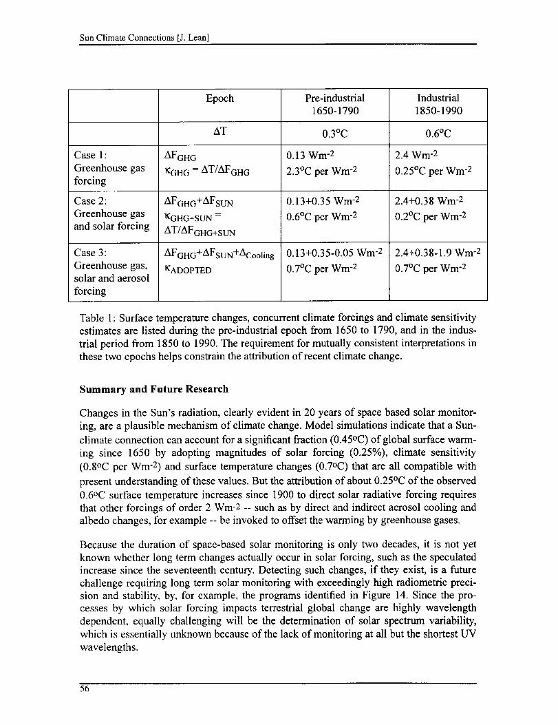
SunClimateConnections[J.Lean]

Case1:Greenhousegasforcing

Case2:Greenhousegasandsolarforcing

Case3:Greenhousegas,solarandaerosolforcing

Epoch

AT

AFGHG

KGHG = AT/AFGH G

AFGHG+AFsuN

KGHG+SU N =

AT/AFGHG+SUN

AFGHG+AFsuN+ACooling

I(ADOPTED

Pre-industrial

1650-1790

0.3°C

0.13 Wm -2

2.3°C per Wm -2

0.13+0.35 Wm -2

0.6°C per Wm -2

0.13+0.35-0.05 Wm -2

0.7°C per Wm -2

Industrial

1850-1990

0.6°C

2.4 Wm -2

0.25°C per Wm -2

2.4+0.38 Wm -2

0.2°C per Wm -2

2.4+0.38-1.9 Wm -2

0.7°C per Wm -2

Table 1 : Surface temperature changes, concurrent climate forcings and climate sensitivity

estimates are listed during the pre-industrial epoch from 1650 to 1790, and in the indus-

trial period from 1850 to 1990. The requirement for mutually consistent interpretations in

these two epochs helps constrain the attribution of recent climate change.

Summary and Future Research

Changes in the Sun's radiation, clearly evident in 20 years of space based solar monitor-

ing, are a plausible mechanism of climate change. Model simulations indicate that a Sun-

climate connection can account for a significant fraction (0.45°C) of global surface warm-

ing since 1650 by adopting magnitudes of solar forcing (0.25%), climate sensitivity

(0.8oC per Wm -2) and surface temperature changes (0.7oC) that are all compatible with

present understanding of these values. But the attribution of about 0.25°C of the observed

0.6oC surface temperature increases since 1900 to direct solar radiative forcing requires

that other forcings of order 2 Wm-2 -- such as by direct and indirect aerosol cooling and

albedo changes, for example -- be invoked to offset the warming by greenhouse gases.

Because the duration of space-based solar monitoring is only two decades, it is not yet

known whether long term changes actually occur in solar forcing, such as the speculated

increase since the seventeenth century. Detecting such changes, if they exist, is a future

challenge requiring long term solar monitoring with exceedingly high radiometric preci-

sion and stability, by, for example, the programs identified in Figure 14. Since the pro-

cesses by which solar forcing impacts terrestrial global change are highly wavelength

dependent, equally challenging will be the determination of solar spectrum variability,

which is essentially unknown because of the lack of monitoring at all but the shortest UV

wavelengths.

56


Not known at all, yet, is the mutual impact of the various forcings on the ability of the cli-

mate to respond to each -- so that, for example, might solar forcing in the pre-industrial

epoch have impacted climate differently than in the present era of large greenhouse gas

and aerosol concentrations.'? Also lacking is adequate specification of indirect solar forc-

ings via UV modulation of ozone and the middle atmosphere and by modulation of ener-

getic particles in the atmosphere that affect cloud formation processes. Pathways that

facilitate indirect solar UV radiative impacts on climate are known but sensitivities in

existing models are smaller than empirical evidence suggests. In the third case, both the

physical pathways and the sensitivities need better specification.

I I , i , I

1980 2000

IIIIIIIII IIII IIIIIIIII IIII IIIII NPOESS

2020 2040YEAR

Figure 14: Future missions

Related Publications

Climate Change 1994. Radiative Forcing of Climate Change and An Evaluation of the

IPCC IS92 Emission Scenarios, Intergovernmental Panel on Climate Change (IPCC),

1995, J.T. Houghton et al., Eds., Cambridge University Press.

The Sun's Variable Radiation and its Relevance for Earth, J. Lean, 1997, Annual Review

of Astronomy and Astrophysics, 35, 33-67.

Climate Forcing by Changing Solar Radiation, J. Lean and D. Rind, 1998, Journal of Cli-

mate, 1 l, 3069-3094.

Evaluating Sun-Climate Relationships Since the Little Ice Age, J. Lean and D. Rind, 1999,

Journal of Atmospheric and Terrestrial Physics, 61, 25-36.

Simulated Time-dependent Climate Response to Solar Radiative Forcing Since 1600, D.

Rind, J. Lean and R. Healy, 1999, Journal of Geophysical Research, 104, 1973-1990.

57


The Role of the Sun in Climate Change, D. V. Hoyt and K. H. Schatten, 1997, Oxford Uni-

versity Press.

Simulations of the Influence of Solar Radiation Variations on the Global Climate with an

Ocean-Atmosphere General Circulation Model, U.Cubasch et al., 1997, Climate Dynam-

ics, 13,757-767.

58

Seasonal to Interannual Climate Variability and Predictability [J. Shukla]

SEASONAL TO INTERANNUAL CLIMATE - . yVARIABILITYAND PREDICTABILITY /" fj " "/_

Jagadish Shukla

George Mason University (GMU)

Center for Ocean-Land -Atmosphere Studies (COLA)

([email protected])

Introduction

It is well known that day-to-day changes of detailed weather can not be predicted beyond

a few weeks because of chaotic dynamics which can amplify even small initial errors due

to incorrect observations used for defining the initial state of the atmosphere, or imperfect

governing equations used for making predictions. However it is now well established that

although detailed day-to-day weather cannot be predicted, seasonal mean circulation and

rainfall anomalies can be predicted through the influence of the boundary conditions at the

Earth's surface (sea surface temperature (SST), soil wetness, snow etc.), if these boundary

conditions can be predicted in advance. The causes of seasonal and interannual variability

of the atmospheric circulation and rainfall can be explained by the following three mecha-

nisms: internal dynamics of atmosphere, ocean-land interaction and ocean-atmosphere

interaction. Although the three processes operate together, and the observed seasonal and

interannual variability is a consequence of interactions among them, for conceptual sim-

plicity, it is possible to design numerical experiments to determine what fraction of vari-

ability is caused by each of the three processes. Large number of such experiments have

carried out during the past 25 years. Based on a very large number of observational and

modeling studies, it is now well established that changes in the boundary conditions of

SST, soil wetness, snow cover, etc. can produce large and systematic changes in atmo-

spheric circulation.

This is particularly true for the tropical region where flow patterns are so strongly forced

by SST that there is almost no sensitivity to changes in the initial conditions. This is a

unique and fundamental property of the tropical atmosphere. Likewise the tropical

oceans have a unique property that tropical sea surface temperature is almost completely

determined by the overlying atmospheric forcing. A combination of these unique proper-

ties of atmosphere and ocean make it possible to predict tropical SST variations, and

therefore, tropical circulation and rainfall at seasonal to interannual time scales. More

recently it has also been found that if tropical SST changes are quite large, even the extra-

tropical circulation over certain regions can be predicted at seasonal to interannual time

seales.

In addition to major advances in our understanding of the predictability of seasonal to

interannual variations, there is also an in-situ and space observing system which allows a

near real time description of the three dimensional structures of the tropical Pacific ocean.

Measurements of sea level, SST and surface wind from satellites combined with subsur-

face measurements from an array of moored buoys makes it possible to define dynami-

cally consistent initial conditions for integration of coupled models.

59

Seasonal to Interannual Climate Variability and Predictability [J. Shukla] -_

In this paper we present two major results: 1. We show that the tropical atmosphere (and

ocean) has unique property of showing no sensitivity to changes in the initial conditions

(exception to chaos). 2. We show that by combining a hierarchy of models, it is possible

to predict regional climate anomalies at seasonal to interannual time scales. We present a

case study for January through March average conditions over North America region.

First tropical Pacific sea surface temperature (SST) is predicted by coupled ocean-atmo-

sphere model which is used to statistically specify global SST. The predicted SST is used

to force a global atmospheric model. A high resolution limited area model (ETA model)

for which lateral boundary conditions are prescribed from the output of the global atmo-

spheric model is used to calculate regional climate anomalies over North America.

Results

In this paper, we show 6-9 month forecasts of surface air temperature and precipitation in

North America for a three month average conditions during January through March, 1998,

using a two-tiered approach. In the first tier, a coupled ocean-atmosphere model is used to

predict the tropical pacific SST anomaly several seasons in advance. A higher resolution

global atmospheric general circulation model (AGCM) is used to predict the seasonal

mean circulation anomalies several months in advance in the second tier.

We provide evidence that the two-tiered approach can be extended, using nested regional

climate models, to produce accurate regional climate predictions. The models used in the

two-tiered approach and nested regional climate simulation have significantly improved in

recent years to a level that makes seasonal prediction feasible.

The tropical Pacific SST pattern was predicted for up to 9 months in advance using a cou-

pled ocean-atmosphere model with available input data at the time of the forecast (June,

July, August, 1997). Multiple realizations of the coupled model forecast were averaged to

produce an ensemble mean SST forecast that was then statistically extended to predict the

global SST anomaly. The latter was added to an observed climatology for global SST and

used as a lower boundary condition for an ensemble of integrations of the global atmo-

spheric model. Each of the global integrations was used to provide the lateral boundary

conditions for a companion integration of a regional climate model. The ensembles of

global and regional model predictions were made at least 6-9 months prior to the verifica-tion time of the forecasts.

The Tropical Pacific SST Forecast

The SST forecast produced by the coupled model and subsequent statistical projections

shown in Figure 1, called for an unprecedented, anomalously warm surface temperature in

the tropical eastern and central Pacific. The predicted warmer than normal water in the

Pacific was located east of the dateline along the equator and extended about 5o-10 o north

and south of the equator. The peak SST value forecast by this model was about 3oC abovenormal.

60

SeasonaltoInterannualClimateVariabilityandPredictability[J.Shukla]

Up to the time that the forecast was made, during the ENSO (E1-Nifio Southem Oscilla-

tion) warm event the model had been quite accurate in predicting the onset and rapid

increase of the SST anomaly, although its prediction of the magnitude of the maximum

anomaly was substantially smaller than observed. The JFM98 forecast made six months

in advance was quite accurate in terms of amplitude, phase relative to the annual cycle and

spatial pattern. The predicted maximum anomaly was west of the observed maximum and

fell short of the observed amplitude by about loC. Compared to similar predictions and

simulations made prior to this one, the forecast was considered to be quite accurate and

generally deemed successful.

Sea Suffaee Temperatt Anomaly ForecastWhtt_ (Jan-Feb-Mar) 1998

8ON"

|

Figure 1: Forecast SSTA for January - March 1998 for the global (non-polar) oceans pro-

duced by the application of statistical projections to the tropical Pacific SSTA produced by

the Tropical Pacific coupled model. The contour interval is 0.5°C with red shading for posi-

tive departures from normal and blue shading for negative departures.

The Surface Air Temperature over North America

The model-based SST forecast was applied as a lower boundary condition to the COLA

atmospheric circulation model to produce an ensemble of nine forecasts. The ensemble

members were generated by initializing the model with slightly different initial conditions

to provide some measure of the uncertainty of the forecast. The model ensemble mean

forecast for surface air temperature (Figure 2) had a generally warmer than normal winter

61


for most of northern North America. Positive departures form normal are shaded in red,

and negative departures are shaded in blue. With the exception of the Atlantic coast, parts

of the Gulf of Mexico coast, and the southern parts of the southwestern states of the U.S.,the entire continental U.S. and most of Canada were forecast to have seasonal mean tem-

peratures (January through March 1998) more than 1oC (2oF) above normal. The largest

departures from normal in the U.S. were predicted to occur in the northern plains states

(Minnesota, the Dakotas and Montana) with seasonal mean temperature more than 3°C

(6oF) above normal. In Canada, anomalous temperatures more than 6oC (12oF) abovenormal were forecast for Manitoba and the Northwest Territories. For winters in central

North America, the historical record of observations indicates that seasonal mean anoma-

lies of more than 3oC occur less than 15% of the time, and 6oC above normal for entire

season has been observed less 5% of the time, on average.

Precipitation over North America

Typically, predictions of precipitation are less reliable than temperature forecasts due to

the fact that precipitation is more variable, has a smaller spatial correlation scale and is

non-normally distributed. Nevertheless, the large-scale characteristics of precipitation

anomalies are know to be correlated with those of other fields and some information may

be obtained from predictions of seasonal mean precipitation. The seasonal mean predicted

precipitation anomaly for January through March 1998 is shown in Figure 3. Positive

departures form normal (more than usual precipitation) are shaded in green, and negative

anomalies are shaded in yellow. The main features of the anomaly pattern are a swath of

positive anomalies to the south and a band of negative anomalies to the north. The posi-

tive anomalies (more than 1 mm day-I or 3.5 inches for the entire season above normal)

extend form the Pacific northwest states of the U.S., through California and the southwest

U.S. into Mexico, and along the Gulf of Mexico into the southeast U.S. The band of nega-

tive departures from normal extends from the Pacific coast of C_a-aada through the norther

plains of the Great Lakes states of the U.S. into the maritime provinces of Canada. The

largest departures form normal are forecast for northern California and central Mexico,

but a significant region of more than normal precipitation (1.5 mm day-1 or 5 inches above

normal) extends through the southwest states (southern California, Arizona, New Mexico,

and Texas) and the Gulf states (Louisiana, Mississippi, Alabama, Georgia, and Florida).

Forecasts for Alaska and Hawaii (not shown) are near normal and below normal precipita-

tions respectively. The forecast for California, Mexico and the southwest U.S. precipita-

tion amount was nearly unprecedented compared to the historical record of observations,

occurring less than 1% of the time or once per century.

62


Surface Ternpera_,ure Anomaly (deg F)Winter (JFM) 1998

Center for Ocean-Land-Atmosphere Studies (COLA) Forecast

Figure 2: Forecast surface air temperature anomaly for January - March 1998 produced bythe COLA atmospheric general circulation model. (AGCM) The lower boundary conditionapplied at oceanic gridpoints was the SST obtained by adding the SSTA shown Figure 1 to theobserved climatological mean SST. The ensemble mean of nine forecasts with slightly per-turbed initial conditions (based on atmospheric observations for mid-December) is shown.The anomaly is defined relative to the COLAAGCM climatological mean. The contourinterval is I°C with red shading for positive departures from normal and blue shading fornegative departures.

63


Precipitation .Anomaly (Inches)Winter (JFM) t998

Center for Ocean-Lend-Atmosphere Studies (COLA) Forecast

Figure 3: Forecast precipitation anomaly for January - March 1998 produced by the COLA

atmospheric general circulation model. Contours are shown 0, q0.5, ql, q2, q3, q4, and q5

mm/day with green shading for positive departures from normal and yellow shading for neg-

ative departures.Regional Rainfall Forecasts

Figure 4 shows nine maps each showing the regional model prediction of continental U.S.

precipitation for each of the members of the ensemble in the JFM98 case. It can be seen

that in certain regions there is uncertainty in predicting the regional rainfall. It is therefore

necessary to generate large ensembles so that a reliable probabilistic forecast can be pro-

duced. Figure 5 shows the observed seasonal mean (JFM98) precipitation over the conti-

nental U.S. Three boxes are shown on the map indicating where regional analysis was

performed. Figure 6 shows the daily total rainfall for the southwest (SW) box as observed

and as predicted by global and nested regional models for each day in JFM98. The

regional model forecast is on top, and the global model forecast is on the bottom. The

observed are in the middle for comparison. The figure demonstrates the advantage that the

regional model has for simulating the storminess in that region. The nested regional

model correctly captures the number and intensity of rain events.

64


Jan-Mar 1998 Daily Precipitation: Southwestern US

241z_ Regional Model

20-18"

16-

14-

12-

10"

8"

6"

4"

2"

01JAN 5JAH11JAN16JAN21dAH26.1AH1FEB6FEB 11FEB15FI:'I:I?1FEB,?.6F_tLkR6LIAR11MAR1BMA_1MAR26MAR1998

24j Observed22 PrecipitationZO"

18"

16-

14"

10"

8

6

.I ,,_ . . III i I. ] Ii.i m _ i -- ---- m • ....

19G'fl

24-

2:2-20-

18-

16-

14-

12"

10.-

Globol Model

4.,-t , I t_., il_,. .L Jl I. i , i . •l) -, ....... -r -, -, , -, T ,= , ,-1JAN BJxLH11J_N16_N21JAH2_AH 1FEB 6FEB11FEB1BFI:I:IPlFEB2BFIH]H_R6ktAR11H_el 6M_R21ki_l_6i4_R1998

Center for Oceon-Lond-Atmosphere Studies

Figure 4: Continental U.S. Precipitation predicted by regional model for nine members of

ensemble for JFM98.

6_

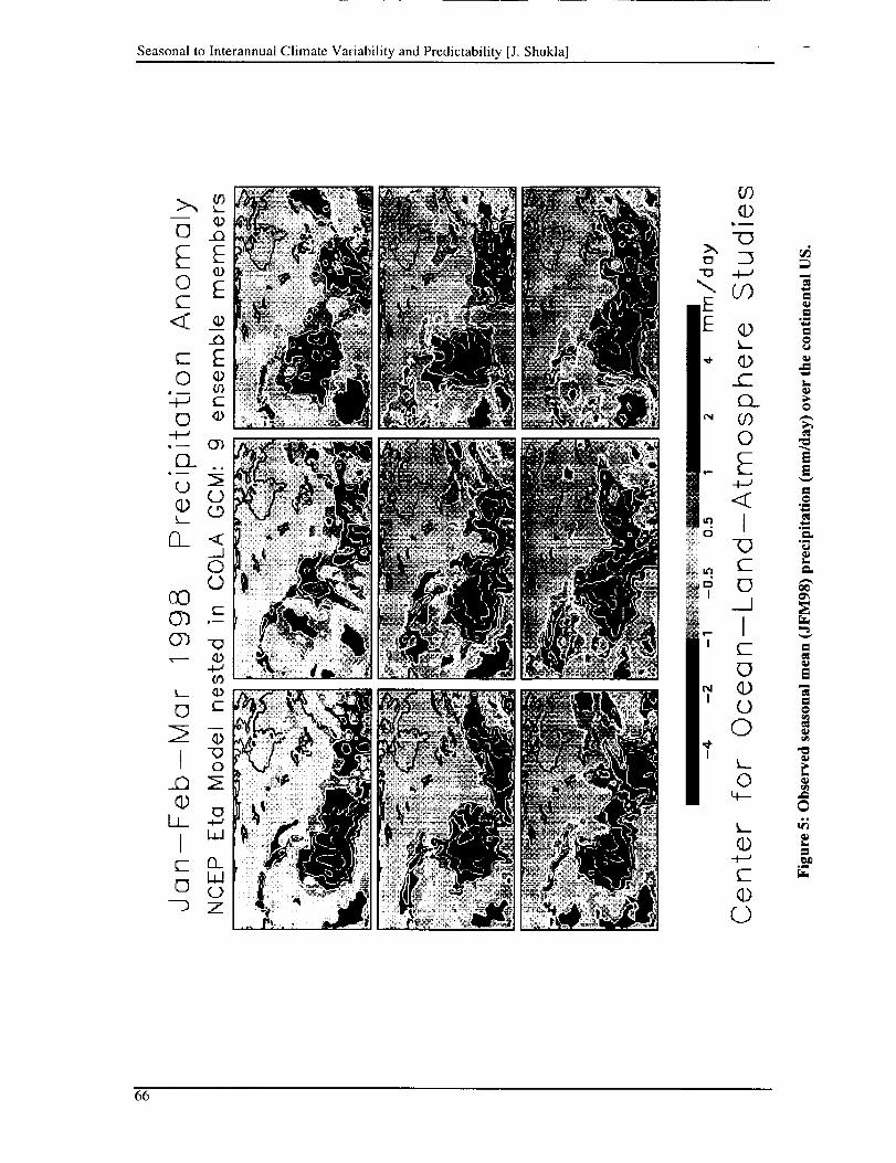
SeasonaltoInterannualClimateVariability and Predictability [J. Shukla]

66


t-

O

1D

Im

U©.k.-

O._

t-- >',u t2tl) 7_

Ii"D

G.)

k_

t-_(D

Z

t_

_t

t_.

_So

,,o o

t. ,,_

m

s_

m

o

N

oE

°_

67


It is difficult to say whether such accurate forecasts can be produced routinely. In this par-

ticular case the large scale flow pattern was predicted with remarkable degree of success

six months in advance. Figure 7 shows three depictions of the 500 mb height anomaly-

observed, predicted at six months lead and hindcast. The latter two were produced using

exactly the same model and initial conditions, but the lower boundary conditions was the

six-month lead SST forecast from the coupled model and the observed SST (hindcast).

The forecast was very good, and the hindcast was even better, showing the potential for

predicting the height anomaly had we predicted the SST perfectly.

Observed (,NCEP), JFM 1998 COLA Model Forecast, JFM 1998

(a) (b)

COLA Model Hindcast, JFM 1998

Figure 4: Observed (a) and six

month lead forecast (b) 500 hPa

height onomaly for JFM 1998;

(c) model hindcast using observed $$T

(c)

Figure 7:JFM98 mean see mb height anomaly: observed (top left); six month forecast (top

right); hindcast (bottom).

Discussion of Uncertainty in Climate Forecasts

In discussion of any climate forecast produced by a numerical model, it must be stressed

that there is a substantial element of uncertainty in any such product. The Earth's climate

is highly variable, and the current stat of the science of climate variations indicates that

only certain regions on the globe and only certain seasons of the year are appreciably pre-

dictable. One of the major advances of climate dynamics is the establishment of a scien-

tific basis for the predictability of seasonal average climate anomalies. Therefore, while

weather fluctuations are known to be predictable beyond about two weeks lead time, cli-

mate variations in the tropics and select regions outside the tropics are predictable on sea-

sonal to interannual time scales. The extratropical climate is highly variable, and the

68


influence of tropical SST anomalies is responsible for only a portion of the observed vari-

ation. Recent research has shown, however, that, in the presence of large tropical SST

anomalies, the seasonal climate over the Pacific-North American region is highly predict-

able. Despite elements of uncertainty, the numerical model can produce a forecast for

each point on the globe for each moment in the future. It is a matter of current scientific

inquiry to interpret the numerical model output in the context of climate uncertainty. In

discussing the results of this study, we emphasize that the results are the products of a

numerical model for which a detailed quantitative analysis of the uncertainty has yet to be

made.

It should also be noted that the prediction methodology employed in this study involves

two distinct numerical model products. The first step of the forecast procedure involves a

coupled ocean-atmosphere model. The inclusion of observational information and the

high degree of predictability of tropical Pacific SST provide a measure of confidence for

the SST anomaly forecast. The final step of the forecast procedure (after the intervening

steps that effectively project the output of the coupled model form tropical Pacific SST to

global SST using statistical techniques based on historical observations) involves a model

of the global atmosphere only. The final step assumes that the SST anomlay forecast pro-

duced in the first four steps is "perfect". We emphasize the differences between the first

step and the final step, because it is important to keep in mind that forecasting tropical

Pacific SST anomalies and forecasting the global effects of those anomalies are distinct.

The two parts of the forecast procedure have different levels of uncertainty and, hence,

different levels of reliability.

The memory required for predicting SST changes reside in the upper ocean. To exploit

the theoretical predictability of the climate system for the benefit of society, it is essential

that in-situ and global observations be combined to define the initial state of the global

atmosphere and upper ocean. Both, the improved models and extensive global observa-

tions are required to produce useful climate forecasts.

69

EI-Nino:Monitoring,Prediction,Applications,Impacts[C.Ropelewski& A.Moura]

EL NII_O: MONITORING, PREDICTION, AND IMPACTS

Chester F. Ropelewski and Antonio D. Moura

International Research Institute for climate prediction

Lamont-Doherty Earth Observatory of Columbia University

[email protected], [email protected]

Introduction

/ 9

e

Interannual variability over the most recent three to four years has provided an unprece-

dented opportunity for the climate community. The recent sequence of La Nifia and E1

Nifio episodes have allowed us to: a) reap the benefits of relatively new ocean observa-

tional systems, b) exercise a new generation of coupled ocean/atmosphere models for

operational seasonal climate predictions and c) initiate development, testing and imple-

mentation of seasonal forecast applications tools. This paper briefly describes some of the

related activities in these areas at the newly formed International Research Institute for cli-

mate prediction.

Monitoring

Over the past two decades significant improvements in real-time monitoring of the climate

have been achieved through collaborative efforts of the international climate community.

Among the most significant of the enhancements to observations was the initiation and

implementation of the Tropical Atmosphere Ocean (TAO) Array of buoys for in situ mea-

surements of the equatorial Pacific Ocean. These measurements have been invaluable for

providing data for analysis and prediction of the Pacific Ocean surface temperature as well

as the thermal substructure. Not only does the TAO array allow climate scientists to mon-

itor the state of the equatorial Pacific but it also provides observational input for data

assimilation systems of coupled numerical ocean/atmosphere models.

The success of the TAO array has led the Global Ocean Observing System (GOOS) to

plan expansions of in situ monitoring into the other ocean basins. The initial deployment

of several buoys as part of the PIRATA array in the equatorial Atlantic is a successful

example of this expansion.

The value of the TAO measurements has been dramatically enhanced through their use in

conjunction with a number of satellite observations. Among these are the NOAA AVHRR

estimates of sea surface temperatures and the TOPEX/POSEIDON estimates of sea level,

Figure 1. Sea level is proportional to the ocean heat content and a proxy for sea surface

temperature, both key variables for monitoring the equatorial oceans. Thus the satellitemeasurements allow climate scientists access to independent, continuous, high-resolution

measurements of the ocean with global coverage.

71

FA-Nincc Mc, nitc, rin,-. Prediction. Applications. Impacts [C. Ropclevcski & A. Moura]

Figure 1: Sea surface height anomaly estimated by TOPEX/POSEIDON. Negative (positive)

height anomalies are in blue (red). Source: JPL/NASA

72

EI-Nino: Monitoring, Prediction, Applications, Impacts [C. Ropelewski & A. Moura]

The E1 Nifio/Southern Oscillation (ENSO) has been extremely active since the early

1980's. In particular, an alternating sequence of La Nifia and E1 Nifio conditions starting

in 1996 has been accompanied by an extraordinary sequence of rainfall and temperature

extremes over many regions of the globe. Much of the ENSO-related activity has been

described in detail elsewhere. Below, we briefly summarize the evolution of the ENSO

episodes over this remarkable period.

After a nearly continuous period of E1 Nifio episodes and El Nifio-like conditions for the

first half of the 1990's La Nifia conditions appeared late in 1995. La Nifia conditions had

peaked in 1996 and climate forecasters were already turning their attention to the possibil-

ity yet another El Nifio episode forming in 1997. By early in the year (1997) most models

and empirical forecasts were indicating the inception and evolution of a major E1 Nifio

episode. The tbrecasts were realized with the appearance of extremely strong E1 Nifio

conditions that dominated the global climate throughout 1997 in into early 1998. This "El

Nifio of the century" grew to surpass the great 1982/83 El Nifio in magnitude and then

gave way to moderate La Nifia, cold episode conditions, by mid-1998. The sequence of

events starting in early 1996 is well documented by the alternating cold (La Nifia) sea sur-

face temperature and warm (El Nifio) sea surface temperature in the equatorial Pacific,

Figure 2.

For the most part the rainfall and surface temperature patterns followed those expected

during warm and cold episodes e.g., Figure 3. In particular, a series of extremely wet and

dry years in the far western Pacific, including Indonesia, were mirrored by a series of

extremely dry and wet years from just east of the dateline eastward across the Pacific.

These rainfall extremes were associated with a number of significant disruptions to the

economy and well being of several Pacific nations.

Prediction

The highly active period of ENSO variability starting in the mid-1990s has provided a

challenging test bed tbr the developing coupled ocean-atmosphere numerical models. For

the first time, these models were being exercised for real-time climate prediction. Much to

their credit this generation of models did very well in forecasting the continued evolution

of equatorial Pacific sea surface temperatures, Numerical forecasts of seasonal patterns of

temperature and precipitation anomalies based on predicted sea surface temperature, while

far t?om perfect, also provided useful climate information to a wide range of users.

Not all of the rainfall and temperature anomaly patterns typically experienced during

ENSO warm episodes occurred with the 1997/98 ENSO. In particular, the 1997 monsoon

seasons in Australia and India averaged near the long term mean rainfall amount despite

fears that this strong E1 Nifio would bring disastrous droughts as they did in Australia dur-

ing the 1982/1983 warm episode.

O11 the other hand some of the ENSO signals were much stronger than had been expected.

Eastern equatorial Africa, Kenya, southern Somalia, the Ethiopian Highlands and north-

eastern Tanzania experienced extremely heavy rainfall in late 1997 into early 1998. While

73

El-Nines: Monitoring, Prediction. Applications, Impacts [C. Ropelcwski & A. Moural

excess rainfall is expected in much of eastern equatorial Africa area during El Nifio years

the rainfall during tile episode exceeded previous records at several stations and was asso-

ciated with widespread flooding.

One of the lessons learned for seasonal climate forecasting is that regional i.e., ocean

basin-scale, sea surface temperature anomalies can have a strong influence on local and

regional atmospheric circulation and rainllall patterns. One example of this was an area of

strong positive sea surface temperature anomalies in the Indian Ocean. The strong Indian

Ocean temperature anomalies are thought to have been partially responsible not only for

the near average summer monsoon rainfall in India and Australia but also for the

extremely heavy rainfall in eastern equatorial Africa. The IRI Net Assessment forecast for

Africa for the October through December period 1997, Fig.4, captured most of the major

rainfall anomalies, in part, because strong positive Indian Ocean temperature anomalies

were included in the numerical model runs that formed the basis for the Net Assessment.

Sea-Surface Temperature (C)

:C'----

....ti ........i........:.....i

3O

29

28

Temperature Anomaly (C)

3

2

1

0.5

-0,5

-1

-2

-3

1BOw 14Dw 120w IOOw 8Qw

CLIMATE PREDICTION CENTER/NCEP

Figure 2: Time-longitude cross section of monthly mean (top) and anomalous (bottom) sea

surface temperatures averaged over a band 5 degrees on either side of the equator. Dashed

lines indicate negative anomalies. (Original analysis from CPC Climate Diagnostics Bulletin).

74

EI-Nino:Monitoring,Prediction,Applications,Impacts[C.Ropelewski& A.Moura]

O

_.._.

O

°n,i

o t<_

o,,,i

Q ca ;a,,

m

Q

**u

r_ t_

N

75

EI-Nino: Monitoring, Prediction, Applications, hnpacts [C. Ropelewski & A. Moura]

IRI IN'rERNA'rl0NAL RESEARCH IN$'rlTUT_FOR CLIMATE PREDICTION

E'_PERI_IENTAL CLIMATE FO_EC._ST DIVI810N

IRI RAINFALL FORECAST FOR OBSERVED RAINFALL FOR

OCT-DEC 1997 (ISSUED OCT. 1, 1997_ OCT-DEC 1997 (NCEPICPC)_o,. f t.ea.._._.

'_I 253_I_a_ll ,a,

oi [0

IO, I

20i

40_tW_ O_ 30, 601E E

nupmluc ueu /I utL_-:';r".-sJ.-_u"orecas"ne" asmt a_ _ 1_ Im1_ 7= -,_ _ Io

Figure 4: The IRI Net Assessment Forecast for Africa during the October through December

1997 season (left) and analysis of observed rainfall (right) for the same season.

During 1998 the equatorial Pacific sea surface temperatures fell rapidly as E1 Nifio condi-

tions gave way to La Nifia. However, the far eastern Pacific sea surface temperatures

remained above average through the year. During late February and early March of 1999

these lingering warmer than average coastal ocean temperatures gave some concern that

El Nifio was back despite continuing La Nifia conditions in the central equatorial Pacific.

Concern was heightened by reports of rainfall in Piura and other locations that generally

received no rain during this of year. These concerns were alleviated by the end of March

when the unusual rainfall ceased and the positive temperature anomalies declined alongthe South American Coast.

Applications

The application of climate data, intormation, and predictions spans a very broad range of

disciplines at the interlaces between climate tbrecasting and climate-related economic and

social issues. The application of climate information, including forecasts and assess-

ments, can have an influence on policy and decision-making. Climate-applications areas

include agronomy, hydrology, public health, emergency management, fisheries, econom-

ics, public policy, and anthropology, and cut across public and private sectors. The initial

efforts of the IRI's Applications Research Division include the identification of several

pilot applications activities. Among the goals of these pilot applications are the develop-

ment, utilization and assessment of experimental end-to-end prediction systems i.e., from

76


modeling research and experimental climate forecasts to development and implementation

of applications with feed back from the users. The pilot applications projects necessarily

involve active participation of researchers, technical experts, and decision-makers from

the relevant target regions.

In one pilot project the IRI Applications Research Division has been working with various

components of the South American fisheries. This project, begun in 1997, was sparked by

the initiative of the end-users for better and more relevant climate information. Early

results have identified the potential for increased use of climate forecasts by the fisheries

sector. Work is continuing on several aspects of the problem including studies of the

quantitative link between the biology and the climate variability.

The negative consequences of El Nifio on small pelagic fisheries in Peru have been well

documented in previous episodes. However, the IRI pilot project has already revealed

some subtle and complex variations in the relationship between catch, climate and subse-

quent re-actions by the fisheries. For example, during the relatively favorable 1996 La

Nifia season a fairly substantial catch of anchovy was documented, Figure 5. (Note: There

is usually a "ban" on fishing during the February to March and July to September period,

accounting for the low catch values during those months.) During April and May of 1997

the evolving E1 Nifio forced the anchovy stocks to concentrate closer to shore in ever

shrinking areas of relatively cold nutrient-rich water. This made fishing more efficient and

resulted in an even larger overall catch in April and May of 1997 than in the previous year.

The May 1997 catch was down from the April catch primarily because of a short lived (7

day) fishing ban that the government was not able to sustain due to pressure from the

industry. Environmental conditions then led to vertical and horizontal migration of the

small pelagics. Nonetheless, during the first year of the 1997/98 El Nifio there was an

overall increase in catch. Despite this increase in catch the quality of the catch, particu-

larly in 1998, was much less, since it contained a mixture of fish species whose fat and oil

content were well below average. More importantly it led to an over-fishing of commer-

cial species which had survived the harsh conditions of the El Nifio, reducing the capabil-

ity of the stock to recover. This period of over-fishing was followed by a much reduced

catch for the remainder of 1997 and 1998. The overall, long-term, effect of the 1997/98 E1

Nifio remains to be seen but it has already put severe pressures on the fisheries industry of

the area.

77


Peru: Monthly Small Pelagic Catch January 1996

to January 1999

1800

1600

1400

o 1200

1000

800

600

400

200

0

II

lgg6

Jan Apr Jul Oct Jan Apr Jul Oct Jan Apr Jul Oct Jan

Source: Fishrneal Exporters Organization

Figure 5: Time series of small pelagics catch in the eastern Pacific. (Data source: Fishmeal

Exporters Organization)

Summary

During the past two decades seasonal climate prediction has moved from the research lab-

oratory into the realm of operations. Global climate forecasts are being issued regularly at

the IRI and other institutions. The success of this enterprise has depended on the synergy

between improved global observations of the climate system, improved theoretical under-

standing and the emergence of numerical models that predict interannual climate variabil-

ity. A formidable challenge remains in developing and implementing the scientific and

social tools for the efficient and equitable application of climate forecasts to a varied using

community.

Acknowledgments

We wish to acknowledge our IRI colleagues Nick Graham, Simon Mason and Lisa God-

dard for their invaluable input to the prediction discussion and to Kenny Broad for his

vital contribution to the applications discussion. Finally, we thank Brendon Hoch, also at

the IRI, for assistance with the graphics.

78

Cooperation Between Space Agencies and the World Climate Programme (WCRP) [H. Grassl]

CO-OPERATION BETWEEN SPACE AGENCIES AND

THE WORLD CLIMATE RESEARCH PROGRAMME

Hartmut Grassl

World Climate Research Programme (WCRP)

c/o World Meteorological Organization

([email protected])

Global Climate Variability and change as well as many climate processes cannot be under-

stood without earth observation from space by dedicated satellites. Therefore, a close and

long-term co-operation between space agencies and WCRP is a prerequisite in order to

achieve the central goal of WCRP:

To understand and predict - to the extent possible - climate variability and chmate

change including human influences.

Numerous success stories can already be named involving many space agencies (includ-

ing the operational meteorological satellite services), large groups of scientists, in situ data

providers and the co-ordination of the infrastructure of WCRP. These success stories are

of a different kind: Firstly, WCRP as a stimulator of dedicated satellite sensors to under-

stand climate processes, secondly, sub-projects mainly of GEWEX (Global Energy and

Water Cycle Experiment of WCRP) delivering global time series of several climate

parameters, thirdly, improvement of general circulation models for atmosphere and ocean

through validation with satellite data sets, fourthly, trend analyses in the stratosphere and

fifthly, attribution of climate change to causes. I will give an example for each type.

Stimulation of New Sensors for Climate Research

In June 1996, I was writing to the major space agencies on behalf of WCRP's Joint Scien-

tific Committee in order to point to gaps that would remain even after the launch of the

new generation of earth observation satellites (EOS-AM, EOS-PM, ENVISAT, ADEOS

II). In addition, climate research would need:

° Three-dimensional observations of cloud-water and cloud-ice and aerosols in the

atmosphere in order to determine the feedback of clouds to changed temperature

distribution, a prerequisite for the reduction of the uncertainty range of climate

sensitivity to external forcing (mainly due to cloud feedback);

. Upper soil wetness measurements needed for the starting fields of forecast models

trying to exploit the soils' memory for longer-term predictions up to seasonal time-

scales. These starting fields would help in better water resource management;

. Vertical profiles of wind velocity, especially for the tropics, which are needed for

better weather forecasts but also for better water vapour convergence estimates, a

prerequisite to improve parameterizations of precipitation formation in climatemodels.

79

CooperationBetweenSpaceAgenciesandtheWorldClimateProgramme[H.Grassl]

To all threerequestsall major spaceagencieshaverespondedfavorably. Not only planshaveemergedbut alreadyapprovedmissionslike the combinationof PICASSO(ajointNASA/CNES aerosollidar mission)andCLOUDSAT(aNASA cloudradarmission)butalsotheEarthRadiationMission(ERM), studiedby ESA,shouldbenamedhere,sinceitscombinationof radar,lidar andradiometeron thesamesatellitewould facilitatesynergiesbetweenthe different sensors.Hopefully, negotiationsbetweenESA andNASDA willleadto theproperburdensharingfor easierapprovalof themission.

In this context,it is worthmentioningthatWCRPwill alwaysadvocatefor thecontinua-tion of successfulmissions,for example,the radar altimetersonboardTOPEX/POSEI-DON and ERS 1/2). The World OceanCirculationExperiment(WOCE) has,sinceitsinceptionin theearlyeighties,tried hardto getoceantopographymeasurementsduring itsfield phase. In thenineties,with thesensorsmentionedandtheir high quality data,it gotevenmorethananticipated.ThiswasthereasonthatI alsoasked,in the lettermentioned,for agravity missionin orderto fully takeadvantageof thepreciseoceantopographymea-surementsfor oceancirculationstudies,which would needmoreprecisegeoid informa-tion. AgainthemissionsGOCEandGRACEonbothsidesof theAtlantic will help to getthis information.

Global Climate Parameter Data Sets

The close relationship between GEWEX and many space agencies has led to many joint

successes in this field, High up on such a list is the International Satellite Cloud Climatol-

ogy Project (ISCCP) which processes data from all operational meteorological satellites

having a free and open exchange of data policy. Started as an independent scientific activ-

ity in 1982, it soon became the first formal project of WCRP and is now one of several

GEWEX data projects. However, it is the one with the most diverse satellite data assem-

blage and the largest infrastructure. Every six hours since July 1983, a global set of many

cloud parameters is available on a 2.5x2.5 degree grid and several higher resolution sub-

sets exist, for example, for the Baltic Sea catchment, one of the five continental scale

experiments of GEWEX. Input comes from 4 geostationary and two polar orbiting satel-

lites and the algorithms taken have been validated by field experiments, e.g., FIRE (First

ISCCP Regional Experiment). As Figure 1 shows that there is an annual course of cumu-

lus cloud amount and interannual variability in the amount of cloudiness. However a

trend analysis over the time period since 1983 is still not possible, since it had to be

assumed that the mean backscattering of solar radiation by the entire earth has not

changed in this period. The reason being the inadequate in-flight calibration of many sat-

ellite sensors.

Other parameters, for which satellite information is essential and for which we have first

global data sets from GEWEX sub-projects are: Precipitation (monthly means over 10

years for a 2.5x2.5 degree grid), water vapour (only in a five year pilot project for 1998-

192) and surface radiation fluxes. Soon we will have aerosol optical depth, mainly over

oceans, as another importance climate parameter set. This list is not exhaustive and other

global data sets are assembled by other WCRP projects as well, always in close co-opera-

tion with space agencies to the benefit of both partners.

80


R(.J

..... • " • . _., _ • . ,. •

I I "I I I I I I I I I __Z

0 _

-= O

O'e'

1 °I .,I

0 0 0 0 0 Q o

i * I I

F_

I l ' , I f l l l l

I ! I

81

Cooperation Between Space Agencies and the World Climate Programme [H. Grassi]

Validation of Circulation Models

Major progress in modeling of the general circulation in atmosphere and ocean is only

achievable with new observations, both for global as well as regional models. There have

been many steps forward in the validation of models by satellite data or by merged satel-lite and in situ data.

A major step was the availability of the data from the Earth Radiation Budget Experiment

(ERBE), which has led to the validation of the models' radiation budget at the top of the

atmosphere that is a basic capability to be reached by any climate model.

Agreement with the measured radiation budget at the top of the atmosphere is only a nec-

essary, but not sufficient model test and the much more stringent test is a comparison with

the observed surface radiation budget. However, the data set available from the GEWEX

sub-project on Surface Radiation Budget (SRB) is still not precise enough for a really

stringent model test that would, for example, mean the solution of the question on the

amount of solar radiation absorption in a cloudy atmosphere. In addition, precipitation

data sets over oceans are still not advanced enough to be used for a thorough model test.

In other areas, for example the ocean circulation model tests, the satellite-derived ocean

topography has led to major improvements of models since the accuracy was high enough

to detect systematic model errors.

A recent, very promising example of model validation is the comparison between ISCCP

cloudiness information and the vertical and horizontal cloud distribution in the circulation

model of the European Centre for Medium Range Weather Forecasts (ECMWF), showing

that the circulation model realistically develops clouds in the correct height with appropri-

ate optical depth.

Trend Analysis in the Stratosphere

It is well known that the strong ozone depletion in the stratosphere has been followed by

several satellite sensors after it had been detected from ground-based spectral UV-radia-

tion measurements. The less obvious longer-term cooling trend in the lower stratosphere

(larger than the warming trend at the surface, interrupted for a few yeas in 1963, 1982 and

1991 by strong volcanic eruptions) has only recently been established on global scale by a

group in SPARC (Stratospheric Processes and their Role in Climate) through the merging

of all available data sets from radiosondes and satellite sensors. The combination of ozone

trend, greenhouse gas trends, and temperature trend in the lower stratosphere has allowed

for the fist time, with the help of model calculations, to attribute the temperature trend to

certain causes:

The significant cooling trend in the lower stratosphere in mid- and high latitudes during

the recent decades is largely due to ozone depletion and to a lesser extent to the increase

in long-lived greenhouse gas concentrations.

82


Integrated Observing Strategy (IGOS)

The office of the World Climate Research Programme in Geneva is a partner in IGOS.

IGOS was started by the space agencies through the Committee on Earth Observing Satel-

lites (CEOS), but is now a joint undertaking by space agencies, several UN agencies and

the global change research programmes, IGBP and WCRP. In this respect, it should:

• formulate requirements to be met for certain climate parameters;

• help to identify the gaps in observing systems related to climate parameters

through contributions to the IGOS pilot projects;

• contribute to measures to fill the gaps identified.

At present, WCRP is involved in three of the six IGOS pilot projects, namely GODAE

(Global Ocean Data Assimilation Experiment), the Ozone Project and the Disaster Man-

agement Support Project. While WCRP was setting the stage through its projects TOGA

and WOCE for GODAE and will systematically contribute through the Ocean Observing

Panel for Climate (OOPC) to its implementation, it is contributing to the Ozone Project

mainly by formulation of requirements to be met for a sufficient ozone monitoring and an

attribution of causes to observed changes. Concerning the Disaster Management Support

Project, WCRP has again set the stage through the breakthrough to seasonal climate

anomaly predictions (in the project TOGA) which help to prevent disaster following

droughts, still the most important natural disaster affecting mankind. Improvement of sea-

sonal to interannual predictions of climate variability, a major goal of CLIVAR (Climate

Variability and Predictability study of WCRP) is - maybe - the strongest contribution todisaster prevention.

In view of all these joint and successful activities, we should not only look forward to con-

tinued co-operation between space agencies and the World Climate Research Programme,

but we must co-operate in even more fields.

83

REPORT DOCUMENTATION PAGE Fo;mApprove_OMB No. 0704-0188

Public reporting burden for this coflectionof information is estimated to average 1 hourper response, including the time for reviewing instructions, searching existingdata sources,gathering and maintaining the data needed, and completing and reviewing the collection of information, Send comments regarding this burden estimate or any other aspect of this

collection of information,includingsuggestions for reducing this burden, to Washington Headquarters Services, Directorate for Information Operations and Reports, 1215 Jefferson

Davis Highway, Suite 1204, Arlington, VA 22202-4302, and to the Office of Management and Budget, Paperwork Reduction Project (0704-0188), Washington, DC 20503.

1. AGENCY USE ONLY (Leave blank) 2. REPORT DATE | 3. REPORT TYPE AND DATES COVERED

July 1999 I Conference Publication4. TITLE AND SUBTITLE 5. FUNDING NUMBERS

NASA Scientific Forum on Climate Variability and Global ChangeUNISPACE III Code 930.5

6. AUTHOR(S)

Robert A. Schiffer and Sushel Unninayar

7, PERFORMING ORGANIZATION NAME(S) AND ADDRESS (ES) 8. PEFORMING ORGANIZATIONREPORT NUMBER

Earth and Space Data Computing Division

Goddard Space Flight Center 99A01344

Greenbelt, Maryland 20771

9. SPONSORING / MONITORING AGENCY NAME(S) AND ADDRESS (ES) 10. SPONSORING / MONITORINGAGENCY REPORT NUMBER

National Aeronautics and Space Administration

Washington, DC 20546-0001 CP-1999-209240

11. SUPPLEMENTARY NOTESThird United Nations Conference on the Exploration and Peaceful Uses of Outer Space, July 19-30, 1999.

Published by NASA as a contribution to United Nations Office of Outer Space Affairs for UNISPACE III.

12a. DISTRIBUTION I AVAILABILITY STATEMENT 12b, DISTRIBUTION CODE

Unclassified-Unlimited

Subject Category: 47

Report available from the NASA Center for AeroSpace Information,

7121 Standard Drive, Hanover, MD 21076-1320. (301) 621-0390.

13. ABSTRACT (Maximum 200 words)

The Forum on Climate Variability and Global Change is intended to provide a glimpse into some of the ad-

vances made in our understanding of key scientific and environmental issues resulting primarily from improved

observations and modeling on a global basis. This publication contains the papers presented at the forum.

14. SUBJECT TERMS

Climate variability, Global change, EI-Nino, Southern Oscillation, La Nina

17. SECURITY CLASSIFICATION 18. SECURITY CLASSIFICATION 19. SECURITY CLASSIFICATIONOF REPORT OF THIS PAGE OF ABSTRACT

Unclassified Unclassified Unclassified

NSN 7540-01-280-5500

15, NUMBER OF PAGES

8416. PRICE CODE

i

20. LIMITATION OF ABSTRACT

UL

Standard Form 298 fReT. 2-89)

Unispace-III/NASA Scientific Forum on Climate Variability and Global Change (20 .luly 99,

Vienna, Austria

Program Plan

9.00-9.15 am: Introduction(Chair/Co-Chair/Rapporteur): Climate and Global Change Issues. [Dr.

Robert Schiffer (NASA/HQ), Dr. Sushel Unninayar (NASA/GSFC)]

9.15-9.55 am: Ozone Depletion, UVB and Atmospheric Chemistry. [Dr. Richard Stolarski

(NASA/GSFC)]

9.55-10.35 am: Global Climate System Change and Observations. [Dr. Kevin Trenberth (NCAR)]

10.35-11.15 am: Predicting Decade-to-Century Climate Change: Prospects for Improving Models. [Dr.

Richard Somerville (SIO)]

11.15-11.55 am: Sun-Climate Connections. [Dr. Judith Lean (NRL)]

12.00-2.30 pm ............................. LUNCH ...................................

2.30-3.10 pm: Seasonal to Interannual Climate Variability and Predictability. [Dr. Jagadish Shukla

(COLA)]

3.10-3.50 pm: El-Nino: Monitoring, Prediction, Applications, Impacts. [Dr. Chester Ropelewski & Dr.

Antonio Moura (IRI)]

3.50-4.30 pm: Understanding/Predicting Changes in Terrestrial and Marine Ecosystems; Links with the

Global Carbon Cycle. [Dr. Tony Janetos (WRI)]

4.30-4.45 pm: Cooperation Between Space Agencies and the World Climate Programme (WCRP). [Dr.Hartmut Grassl (WMO/WCRP)]

4.45-5.00 pm: Closing Remarks: Contemporary Global Change Science. [Dr. Ghassem Asrar, Associate

Administrator for Earth Science, NASA/HQ]

5.00-5.30 pm: Panel Discussions: All Keynote Speakers and All Participants

[Development of recommendations to be submitted to UN/COPUOS/Agenda Item 7].................................................................................................................

5.30-6.30 pm: RECEPTION (Astronauts and Cosmonauts Event)+++++++++++++++++++++++++++++++++++++++++++++++++++++++++++++++++++

For more details on UNISPACE-III see UN/OOSA Website: [http://www.un.or.at/OOSA/unisp-3/]

Acronyms:

COLA: Center for Ocean-Land--Atmosphere Studies

GSFC: Goddard Space Flight CenterIRI: International Research Institute for Climate Prediction

NASA: National Aeronautics and Space Administration

NCAR: National Center for Atmospheric Science

NRL: Naval Research Laboratory

SIO: Scripps Institute for Oceanography

WCRP: World Climate Research Programme

WMO: World Meteorological Organization

?r=19990064061 2018-01-22t18:55:46+00:00z · pdf fileas a contribution to ... human shelter,...

Documents