Learning in Artificial Neural Systems

Christopher J. Matheus and William E. Hohensee

Inductive Learning Group

Department of Computer Science

University of Hlinois at Urbana-Champaign

1304 West Springfield Avenue

Urbaua, Illinois 61801 USA

Arpanet: (matheus I hohensee)@a.cs.uiuc.edu

Phone: (217) 333-3965

December 1987

Keywords: artificial neural systems, neural networks, connectionism, learning

This report is a slightly modified version of a paper to appear in

Computational Intelligence Journal, Vol. 3, _f-4, 1987.

https://ntrs.nasa.gov/search.jsp?R=19980040349 2019-02-01T13:21:49+00:00Z

Learning in Artificial Neural Systems

Christopher J. Matheus and William E. Hohensee

Computer Science Department

University o/Illinois at Urbana-Champaign

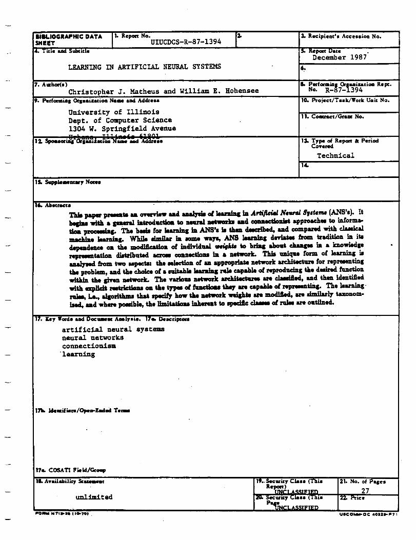
ABSTRACT

paper presents an overview and analylds of learning in Artiftciul Neural System_ (ANS's). It

bef_ns with a general introduction to neural networks and connection_t approaches to informa-tlon proceging. The basis for learning in ANS's is then described, and compared with classicalmachine learning. While similar in some ways, ANS learning deviates from tradition in its

dependence on the modification of individual _eigh_a to bring about changes in a knowledgerepresentation distributed across connections in a network. This unique form of learning isanalysed from two aspects: the selection of an appropriate network architecture for representing

the problem, and the choice of a suitable learning rule capable of reproducing the desired functionwithin the given network. The various network architectures are classified, and then identifiedwith explicit restrictions on the types of functions they are capable of representing. The learningrules, i.e., algorithms that specify how the network weights are modified, are similarly taxonom-ised, and where possible, the limitations inherent to specific classes of rules are outlined.

1. Introduction

Neural networks, parallel distributed processing, and connectlonist models -- which we

shall collectively refer to as Artificial Neural Syatema or ANS's -- represent some of the most

active research areas in artificial intelligence (AI) and cognitive science today. The recent excite-

ment is due to the promising qualities artificial neural systems exhibit in addressing challenging

questions of intelligence. For instance, characteristic of an ANS is its distribution of knowledgeacross a network of units. Since these units act in some ways as evaluators of locally competing

hypotheses, the computational strengths of ANS's can be exploited in the solution of a broad

array of simultaneous constraint satisfaction problems. ANS's have shown promising results for a

number of these problems, including content a_idreuable memory, pattern recognition and asso-

ciation, category formation, speech production, and global optimisation (see Kohonen 1984;

Rumelhart _k McCleUand 1986; Anderson 1977; Sejnowski & Rosenberg 1986; Hopfield & Tank

1986). In addition, the distribution of knowledge across a matrix of individual processing unitsleads to a natural kind of fault tolerance. Since the failure or loss of small portions of the net-

work does not significantly alter overall system performance, ANS's tend to degrade gracefully.

The inherent parallelism of distributed representations make ANS's ideal candidates for imple-

mentation on new parallel hardware architectures. Moreover, as crude approximations to biolog-

ical neural systems, ANS's contribute to a new paradigm for dialogue among many of the discip-

lines of cognitive science. But perhaps the most interesting quality, and the central topic of this

paper, is the way in which learning is effectively accomplished in ANS's through simple, low-level

Learning in Artificial Neural Systemsf

M_theue & Hohensee

learning rules.

Before we examine the low-level details of learning in ANS's, consider first the problem of

learning in general. From one perspective, the goal of a learning system is to acquire a function

that maps input events to output responses. For a given learning problem, a set of inputfeatures defines the multi-dimensionai input space called a "feature space" in which all possible

events exist as vectors. A system's output responses may use this same space or possibly a

separate "concept space" or "hypothesis space" (Rendell 1986). In either case, an ANS, or any

learning system, can be viewed as a black box that learns to map input events to appropriate

output responses.

How then does an ANS differ on this level from other learning approaches? When properly

configured, ANS's are theoretically capable of acquiring any arbitrary mapping function (Volper

& Hampson 1986), and therefore have no inherent representational or learning advantages ordisadvantages compared to traditional machine learning systems. In terms of efficiency, ANS's

can be computationally more expensive (at least when implemented on sequential machines), and

their training sets are frequently larger than required for more traditional methods. In fact, in

certain situations, standard data structures and algorithms can be shown to learn mapping func-

tions with greater efficiency than a typical ANS (Omohundro 1987).

On the other hand, ANS's exhibit interesting and useful learning capabilities. Generaliza-

tions "spontaneously" emerge through an ANS's exposure to, and processing of, input patterns.

In multi-layered ANS's, these generalizations result in the construction of "new terms" for inter-

nal representations, thereby suggesting solutions to the problem of constructive induction (Ren-

dell 1986). The generalisations that occur in some ANS's are remarkably similar to the results oflearning in humans, displaying many of the same strengths and weaknesses. Further study of the

emergent properties of ANS's may therefore lead to a better understanding of the process of

human learning. Finally, while ANS's have already demonstrated useful learning capabilities, the

field is new and may yet hold even greater unexplored insights into computational intelligence

and learning.

This paper presents a general overview of learning within artificial neural systems. It does

not assume familiarity with the terminology or operation of ANS's. Instead, we begin with an

introduction to a simple artificial neural unit (section 2.1) and describe the components of a basic

network configuration (section 2.2). The unique representation of knowledge within ANS's has a

direct bearing on the nature of learning, and we therefore introduce some representational con-

cepts early, in section 2.2. With this background in mind, specific issues surrounding learning in

ANS's are examined. First, we contrast learning in ANS's with learning as it is viewed in tradi-

tionai AI domains (section 3.1). We then separately consider the questions of 1) the learnability

of a function within a network architecture, and 2) learnabUity given a specific learning rule.

Looking first at the representational capabilities, we demonstrate some constraints imposed by

the selection of different network architectures (section 4). Three general classes of learning rulesare then introduced, and the capabilities and limitations of specific rules are considered (section

5). This paper strives to provide an introduction and overview of issues important to practical

learning within ANS's. For a more formal analysis of computability and complexity issues see

(Volper & Hampson 1986; Hampson _k Volper 1986; Egeciogiu eta/. 1986).

2. Art|flelal Neural Systems

The distinguishing feature of Artificial Neural Systems is the use of many simple but highly

interconnected parallel processing units. These units are, to varying degrees, based on the

Learning in Artificial Neural Systenm l_atheus _ Hohensee

functional characteristics of biological neurons. The objective of these systems, however, is gen-

erally not neural modeiling, but rather to utilize the computational characteristics they exhibit.

Useful computational qualities emerge when these simple units are organized into networks. The

nature and arrangement of the connections" between units determines both what types of func-

tions a network is able to compute, and what it is able to learn with respect to a given learning

rule. In this section we will review the basic function of a simple neural unit and discuss how col-

lections of them are organized into networks. In addition, the manner in which knowledge is

represented within a network is described. (The statements made in this section are generaliza-

tions of typical A_NS's and are not intended to be universally applicable to all network designs.)

2.1. An Artlflelal Neural Unit

The principal component of an ANS is its processing unit (see Fig. I). Input signals come

into a unit along weighted connections, or "synapses," from neighboring units, and excite (in the

case of positive links) or inhibit (for negative links) the unit's "firing" activity. The magnitude

of a weight determines how strongly the output of one unit will influence another unit's activity:

the larger the absolute weight between two units the greater is the efficacy of the connection, and

the stronger the influence. Typically, the weighted contributions from all inputs are summed todetermine an activation isle[ for that unit:

input 1 A

w 1

input 2

input n _//wn

output

Fibre i: A prototypic A_NS unit. Inputs from units 1 through n are summed together along

weighted connections, w, to produce an activatlon value. That activation value is then typlcally

thresholded to produce an output value for the unit.

3

Learning in Artificial Neural Systems iVlatheus & Hohensee

a i : ,_ Wlj O/ ,

i

where at is the level of activation of the ith unit, w. k the weight from unit / to unit i, and oi is

the output signal from unit j. While this value represents the unit's "activation," it is not usu-

any the same as the unit's output signal, or. Generally o_ is calculated by applying a non-linear

output function, such as the simple step function:

°i = if a t <_ P

where P is the threshold value at which the unit turns "on." After its calculation, this output

value is transmitted along the weighted outgoing connections to serve as input to subsequent pro-

cesslng units.

Though this simple processing of input signals by an individual unit is basic to all ANS's,

the details of implementation may vary between models. For example, a number of different

output functions have been proposed. Figure 2 depicts the more common of these: a linear out-

put function, the simple step--function, and a sigmoidal output function. The range of output

values assumed by the units may also be varied, with d_erent models choosing among binary,

graded, or continuous values. Some networks further incorporate the effects of activation decay

and internal resistance, modeUing similar functions found in biological neurons. These and other

details are, however, beyond the scope of this paper, and are more fully described in (Rumelhart

McCleUand 1986). What is important to this overview is that the basic operation of an indivi-

dual unit is extremely simple:

1) a level of activity, a,, is calculated from the weighted input signals from other units

2) the unit's output signal, ol, is calculated based on the unit's activation

3) oi is transmitted along links to neighboring units for further processing.

output _/_ output

kput

A. linear function B.

kput

step-function

output f

input

C. sigmoidal function

Figure _.. Output functions.

4

Learning in Artificial Neural Systems h_stheus & Hohensee

2.2. Networks of UnitsAn ANSnetwork is defined by specifying the connections between units. This specification

usually takes the form of a connectivity or weight matriz. Connections are typically unidirec-

tional although bidirectional links are assumed in some models (e.g., Hopfieid 1982). In the most

general case, every unit in the network is connected to every other unit. Such networks are said

to be totally ¢onnecte£ In many ANS's, however, some connections are eliminated in order to

improve performance and simplify learning. Figure 3 shows examples of a totally connected net-work and two networks with restricted architectures. The architecture of an ANS defines the

structure used for knowledge representation and processing. Different architectures imposedifferent biases on the functions that can be represented within the network. As will become evi-

dent, knowledge representation In an ANS is quite different from traditional AI approaches. Twoforms of knowledge representation can be identified within neural w/stems: 1) the state vector of

unit activations, and 2) the representation of the mapping function encoded in the weights. Wewill consider each of these in detail since they play an important role in our later discussions of

learning.

The atate vector consists of the vector of output values (or alternatively, activation values)

taken across all units in the network. It represents the instantaneous chunk of knowledge

currently being processed by the network. For a given architecture, portions of this vector may

be used to represent the input and output of the problem. Thus, as shown in Figures 3b and 3c,

the bottom-layer of the network may represent the input vector, while the top layer encodes the

system's output; together they represent the knowledge structures present in the domain and

range of the mapping relationship to be learned. In some networks, such as the multi-layered

ANS shown in Figure 3c, units exist which serve neither as input nor output. These units arecalled hidden units since they are invisible to the external world. Hidden units are not initially

assigned specific meaning, but rather provide a network with additional degrees of freedom in

A. totally connected

output units

input units

B. single-layered

output units

hidden

units

input units

C. multi-layered

Figure _. Network architectures.

Learning in Artificial Neural Systems Matheus & Hohensee

which to construct useful internal knowledge representations. We will have more to say below

(section 4.2) about the extended representational capability that hidden units provide, as well as

the complications they bring to learning.

The second representational form is of longer duration, lasting beyond the short-term

activation state vector. This persistent knowledge is encoded in the weights between the units,

and it is through the modification of this distributed knowledge structure that learning occurs.

Implicitly represented acroes these connections is the mapping function that defines how a given

input state is translated into its associated output. Because all weights contribute to the

representation, the acquired function is said to be "distributed" across the network, as opposed

to being represented locally by any individual unit. The notion of a distribltted representation is

a matter of much debate and confusion. For a more thorough discussion of this topic the reader

is referred to (Rumelhart eta/. 1986; Hinton 1984).

One aspect of distributed representations relevant to our purposes is that all input/output

pair mappings within the represented function are superimposed one on top of another across the

network weights. In contrast, a symbolic representation will typically use a collection of locally

represented function components. For example, imagine a production system where the mappingfrom a set of inputs to a unique output is encoded by a single rule such as [ IF (flies .TX) AND

(has-/eathere ._X) THEN (isa ?X bir_ ]. The complete mapping function of the learning system is

then represented by a collection of many such individually represented rules. In a network, all of

the necessary rules are implicitly represented across a minole set of weights. This characteristic of

the representation becomes important from a learning perspective. Since learning involves the

changing of weights, and any given weight may participate in the representation of multiple

pieces of information, the learning of new knowledge will often depend upon and alter existingknowledge. It is as if adding the rule [ IF (fliee ?X) AND (mammal E() THEN (_a ?X bat) ] could

somehow affect (for better or worse) the knowledge contained in the isa-bird rule.

2.8. Information Processing

There are two difl_ent methods for processing information in ANS's. The first is called

"settling" and the second "feedforward processing." Which of these methods is used for a

specific ANS depends upon the chosen network model and the nature of the mapping function.

Settling tends to be used primarily with auto-associative networks (discussed below), and usually

in the context of pattern completion or optimization tasks. Processing in these systems begins by

encoding the input vector across the entire state vector. New activation states for the individual

units are then derived as the result of the propagation of signals between units. This iterative

process of computing new states continues until the system "settles" into a stable state where no

further changes are possible. At this point, the final state vector represents the output of the sys-

tem. The manner in which the updating of unit states is conducted again depen.ds upon the

specifics of the model. Some models synchronously update all the units at each time step. Oth-

ers use an asynchronous process and update units semi-randomly. The synchronous approach

has the advantage of simplicity and will often settle more quickly. Asynchronous networks, on

the other hand, are less likely to become trapped in local minima or oscillate perpetually between

two states.

The second general form, feedforward processing, occurs predominately in feedforward,

multi-layered networks. The knowledge structure to be processed is first represented as an

activity pattern across the vector of input units. This information is then propagated through

the weighted connections to the next level of units. The resulting pattern of activity at this layer

Learning in Artificial Neural Systems Mstheus _- Hohensee

is, in turn, passed on to the next higher level. The feedforward processing of information contin-

ues in this step-wise, synchronous manner until a solution is represented as the activity across

the final output layer. It is possible to combine this feedforward processing with "feedback" pro-

ceseing in which information from higher layers feeds back to lower levels. In this type of net-

work (see Fukushima 1986), multiple iterations of the feedf'orward and feedback processes may be

necessary before a stable final output is realized. The network's processing in this case becomes

more like a settling process, terminating when activity stabilizes or diminishes significantly.

|. Learning Issues

We now turn to the issue of learning. Aa stem in the introduction, we have chosen to view

the general problem of learning as the process of acquiring a function that maps input vectors

(stimuli) to output vectors (responses). To learn this mapping function, a learning system

receives a set of training events from which it constructs an internal representation of the func-

tion. Considered at this level, learning in ANS's is no different from learning in more traditional

system. In fact, ANS's can be effectively viewed within the context of traditional machine learn-

ing paradigm, as is done in section 3.1. The similarities between ANS's and traditional

approaches, however, do not carry through to lower levels of analysis where the details of

representation and learning become significant. Section 3.2 considers the importance of the rela-

tionship between representation and learning within ANS's.

|.1. Contrast to Traditional Machine Learning

Machine learning has traditionally been taxonomized into rote learning, learning from

example (supervised learning), and unsupervised learning (Michalski et 4/. 1983). Learning in

ANS's can be viewed from this same general perspective. One class of networks, for example, is

designed to memorize specific patterns which are later recalled when either the same or a closely

related input is presented to the system. Content addressable memories, such as those found in

the Hopfield Network (Hopfield 1982) or some of the modek by (Kohonen 1984), exemplify this

form of rote-like learning. 1 In contrast, many networks learn from examples to map input pat-

terns into a different set of associated output patterns. During learning, a network of this type is

typically provided with an input pattern to which it responds by computing its best guess of the

desired output. A teacher then provides the system with the correct output pattern, allowing the

system to adjust the weights between units, if necessary, to bring its internal representation

closer to the desired result. Rosenblatt's perceptron (1962), Widrow & Hoff's Adeline neuron

(1960), and Sejnowski et al.'s NETtalk system (1986) each exhibit this form of supervised learn-

ins. Still other networks are designed to learn without direct guidance from a teacher, as is the

case in competitive learning systems. In a typical example, exposure to a dynamic input stream

causes individual units to become unique feature detectors of different input qualities, thereby

effectively partitioning the space of events into useful clusters (Kohonen 1977; Rumelhart &

Zipser 1985). The Adaptive Resonance Networks of Carpenter & Groesberg (1986) exhibit a

similar type of unsupervised learning in the induction of category prototypes.

s The memorisation of specific patterns in AN$'s is diEerent from pure rote learning. For instance, generalisations are madeduring learning that influence how unob,m'ved events will be classified. Also, the addition of new memories is z[ected by and mayalter existing memories.

7

Learning in Artificial Neural Systems. 1_stheus _- Hohensee

a.2. Representation versus Learning

Although learning in ANS's can be abstractly viewed from this traditional perspective, there

are significant differences as to how learning is performed when compared with other machine

learning systems. The main distinctions concern two issues at the heart of any learning problem:

the choice of the problem's representation, and the selection or development of a specific learning

procedure. In traditional machine learning, symbolic representations such as first-order predi-

cate calculus, decision trees, version spaces, schema, etc., are used almost universally to represent

knowledge-level information (lVfichaiski et 61. 1983). These representations are the structures

upon which the learning procedures directly operate, modifying them to reflect the results of

classification. The learning algorithms employed by various systems are designed around and

often critically depend upon the underlying representation chosen for the problem. This situa-

tion is the same for ANS's: the learning algorithms are specific to the chosen representation.

The representations used in ANS's, however, are quite different from anything typically found in

traditional machine learning. The distribution of knowledge across weighted connections, as

described above, is a distinguishing quality of ANS's, and it necessitates a unique approach to

learning. 2 More specifically, learning in ANS's is realised through the modification of the connec-

tion weights according to a chosen [earn_ag ru/e. Before reviewing some of the different learning

rules, we will first look more closely at the relationship between representation and learning inANS's.

The issue ofrepresentati0n versus learning in ANS's can be reduced to the following twoconsiderations: 1) the representational capability of the network architecture being used, and 2)

the capacity for learning within that architecture given a specific learning rule. T_e first of theseconcerns whether the architecture of a particular ANS design is capable of representing the func-

tion Which is to be learned. Some architectures impose inherent representational limitations such

that they are incapable of representing certain classes of functions. The classic example of this

problem is the perceptron (Rosenblatt 1962), which is constrained to representing only linearly

separable functions (discussed below). The second issue is, given a suitable network architecture,

does the selected learning rule have the potential for acquiring the desired mapping function?

lVflnsk7 and Papert (1969) demonstrated that any function can be represented by an appropri-

ately chosen network architecture, but they conjectured there would not in general be a pro-

cedure for learning any arbitrary function from examples. The question thus becomes, for a

given network and function, will a particular learning rule be capable of solving the learning

problem? It is sometimes possible to show that a learning rule is guaranteed to converge to the

correct representation if one exists (e.g., the perceptron convergence theorem (_insicy & Papert

1969)), though unfortunately this is not true in general.

4. Representstlonsl Cspsbllltlw

Representational capability and learnkbiUty are concerns central to the problem of learning

in ANS's. In this section we wlil consider the issue of representation within ANS's. Section 5 will

focus on the detalis of learning. For our analysis of representational capabilities it will be con-

veulent to identify two basic classes of ANS architectures m auto-associative networks andhetero-associative networks. We will look at the representational capabilities of these classes

s The claim that the repremmtafiou within ANS's are distributed across weizhts do_ not mean that they cannot represent moreabstract symbolic structures such u trees and schema (see Touretsky 1986). The claim here is that the level at which the lenrninzmethods operate is fundamentally di_erent between cls_.sical machine learning sad ANS's.

g

Learning in Artificial Neural Systems

individually.

h_stheus _k Hohensee

4.1. Representation in Auto-Associative Networks

The auto-_8ociati_e ANS's have a single layer of units and a single layer of weights with no

hierarchical orientation to the network (see Fig. 3a). The major distinguishing quality of this

class of networks is that the input, output, and state vectors are all one and the same, i.e., every

unit of the network participates in the representation of both input and output data (Hinton

1986). This design characteristic means the input and output vectors must be of the same

length, and are usually chosen from the samedomain. Often in these cases the networks aretotally connected and the weighted links between units may be bidirectional. Units may also be

connected to themselves, providing direct "feedback" and thereby allowing a unit's current state

to affect its next state. 3 Indirect feedback is prominent in auto-associative networks, occurring

wherever a cycle exists in the network, as is trivially the case for bidirectional connections.

Computation or processing in an auto-assoclative network is initiated by instantiating an

input pattern across the network units, and then, as described earlier, allowing the system to

iteratively calculate unit activation levels, and propagate outputs through the net until it settles

into a final output state. The output states are the memories stored in the system through learn-

ing. During settling, the input patterns are "attracted" to the closest memory state. 4 An an,I.

ogy is often drawn between this settling process and the search for a minimum in an energy func-

tion. Imagine, for example, an energy surface superimposed over the feature space. Each event

or point in the space is associated with a specific energy value. The memories represented in the

auto-associative network correspond to minima in this energy surface (see Fig. 4). Due to the

nature of the settling procedure, processing of the network causes the system to fall from its ini-

tial state into the closest energy "well."

_'hat, if anything, can be said about the representational constraints of auto-assoclative

networks? Using the analogy of the energy function, it can be shown that auto-associative net-

works are limited to representing mappings which can be defined in terms of the minima of a

quadratic function depicting a continuous energy surface (Egeciogiu et a[. 1986). The complexityof this function is constrained by both the number of units and the range of outputs of the units

(continuous outputs permitting finer resolution than binary-valued units). Because of this qual-

ity of associating an input with the nearest memory image, auto-aasoclative networks have been

used successfully (and almost exclusively) for pattern recognition/completion (Kohonen 1984;

Hopfield 1982), though such networks have also been used to find good approximations to certain

global optimisation problems (Hopfield & Tank 1986).

4.2. Representation tn Het_at|ve Networks

Architectures that explicitly distinguish between input and output units (e.g., Fig.'s 3b &

3c) constitute our second class of networks. They are sometimes called hereTo-associative net-

works because they associate an input pattern presented across a designated layer of input units,

with a specific output pattern across a separate output layer. This di_ers from the auto-

s In soma models this capability for direct feedback k prohibited in ord_ to guarantee stable, non-o6cilltting final states (seeHopfleld lOS|).

4 Closeness can be measured by the Hamming distance between two state vectors in feature spacec

9

Learning in Artificial Neura/Systems Matheus&Hohensee

memory states

Energy

Figure J: Energy surface representing learned memory states. Each well" of the energy

surface represents a final memory state into which the network may settle.

associative networks in that in addition to making a semantic distinction between input and out-

put units, hetero-associative networks impose restrictions on the arrangement of connections

that are permitted. A typical constraint, for example, is that units in one layer project only to

units in subsequent layers. By constraining the network connections the overall number of

weights can be reduced, decreasing the time needed for learning and computation. When these

connections are unidirectional without feeding back to previous layers, computation can be

emciently accomplished using single-pass, feedforward processing. Such constraints on the con-

nectivity of the network, however, can also restrict the class of functions that can be represented.

If we limit our consideration to networks having strictly acyclic, feedi'orward connections,

some specific representational constraints can be identified for the classes of Boolean functions

computable under different hetero-assoeiative architectures. Consider first the simple, hereto-

associative ANS shown in Figure 3b. A single layer of weighted connections serves to ]ink two

distinct input and output layers of the network. The perceptron model (Rosenblatt 1962) was a

single-layered hetero-assoeiative network of this type (with only one output unit), and was one

of the earliest models to demonstrate interesting results. Unfortunately, as a representational

system the perceptron, and other similar models, are severely limited by their architecture.

Single-layered networks are inherently constrained to representing functions whose domain is

linearly separable. This limitation results because a single perceptron of multiple input units and

one binary-valued output unit is simply a linear discriminator that defines a hyperplane splitting

the multi-dimensional feature space into two regions (h_nsky & Papert 1969). This limitation is

depicted graphically in Figure 5a.

To achieve greater representational and functional capability requires the addition of hiddenuni_. As described above, hidden units are isolated from the external world in that they do not

directly participate in the system's input or output. An ANS with hidden units usually have at

least two layers of connecting weights: one layer of weights connecting the input to the hidden

units, the other from the hidden to the output units (see Fig. 3@ ANS's in this class of network

IO

Learning in Artificial Neural Systems _theus 8c Hohenseef

A_ One Weight Layer B. Two Weight Layers C. Three Weight Layers

Hyperpl_e

o/\o

i\

\\

ConTex Regions

C

Unconstrained

Figure 5: Computable output regions for three different network architectures (after

Lippman 1987). 5_ A network composed of one layer of weights is restricted to dividing the

output space into two distinct hyperplanes. 5b: A two-layered network may represent functions

which map into convex open or dosed regions. 5c: A three-layered network given enough hidden

units, is unconstrained and has the capacity to represent any arbitrary function.

11

Learning in Artificial Neural Systems Sstheus _k Hohensee

architecturesare calledmulti-layered,hereto-associativenetworks. Multi-layerednetworks are

the focusof most currentresearch,both because they have extended computational capabilities,

and because the additionofhidden unitsconsiderablycomplicatesthe learningprocess. The

learningproblem that arisesfrom the introductionofhidden unitsisthe credita_signment proS-

lens(Miusky _kPapert 1969). Sincethereisno knowledge of what statea hidden unit"should"

be in,itisdifficultto determine whether a given hidden unitiscontributingpositivelyor nega-

tivelyto the overallperformance ofthe system. The implicationsofthisproblem willbecome

apparent later when we discuss specific learning rules.

A feedforward network with two layers of weights (one layer of hidden units), unlike a

single-layered network, is able to represent any convex--open or closed region in feature space

(see Fig. 5b). For Boolean categories described by Boolean features, a two-layered network can

represent any arbitrary mapping function. This result follows from the fact that 1) any logical

functioncan be implemented as a circuitwith a layerofAND gatesfeedingintoa singleOR gate

(Muroga 1971; Volper _kHampson 1986),and 2)with the appropriatechoiceof thresholds,linear

threshold units can mimic the functions of AND and OR gates. Alternatively, this result is

arrived at by observing that a convex region can be defined by a single unit which AND's the out-

puts from a set of perceptron-like units, forming the intersection of multiple hyperplanes (see

Fig. 5b).

When the input features are multi-valued or continuous, a two-layered network may no

longer be able to adequately represent the desired function. In this case, a three-layered network

may become necessary. A three-layered, feedforward network can be shown to be adequate for

representing any arbitrary function, given enough units at each internal layer (Hanson & Burr

1987; Lippmann 1987). An informal proof of this comes from observing that any geometric

region in a multi--dimensional space can be approximated to an arbitrary degree of accuracy by

ORing the outputs of a collection of two--layered ne.tworks which individually describe an

appropriate set of convex-closed regions in the function domain (see Fig. 5c) (Lippmann 1987).

4.8. Summary of Representational Capabllitles

What the above analysis shows is that the choice of a particular ANS architecture may

result in inherent biases or constraints that restrict the class of representable functions. In the

most general neural network, where every unit is connected to every other unit, there are no

inherent representational biases, other than the obvious limits imposed by the finite number of

units in the network. But while a completely connected ANS can mimic the architecture of any

partially connected network having the same number of units (i.e., by selectively assigning con-

nective links to zero weights), efl|ciency and learnability considerations often disfavor this most

general approach, especially in large networks. Consequently, the network architectures chosen

for practical systems frequently restrict the connections between units. By eliminating potential

connections, however, the resulting architecture may be unable to represent certain function

classes. Provided the network design permits the representation of the problem's mapping func-

tion, a restricted architecture can in many cases improve performance and learning.

6. Learning Rules

Even ifa particularANS architecturehas the theoreticcapabilityto model the desiredfunc-

tion,thereremains the questionofwhether the learningrulethat isused willbe ableto produce

the appropriaterepresentation.Sincelong-term representationsare distributedacrossthe

12

Learning in Artificial Neural Systems MAtheus Jk Hohensee

weights of the interunlt connections, learning new information is accomplished by modifying

these weights in such a way as to improve the desired mapping between input and output vec-

tors. This mapping function is learned by adjusting the weights according to some well defined

learning rule. It will be convenient to identify three general classes of rules. The first, which wewill call correlational rules, determine individual weight changes solely on the basis of levels of

activity between connected units. The second class is the set of error-correc_r_g rules, which relyon external feedback about the desired values of the output units. The third class comprises the

unsuper_ed [earning r_es, in which learning occurs as self-adaptation to detected regularities in

the input space, without direct feedback from a teacher.

It is interesting to note the analogic connection that can be drawn between these classes of

ANS learning rules and traditional learning par_ligms. The correlational rules are frequently

found in auto-associative networks that perform rote-Uke learning of specifc memory states

(Hopfield 1982; Kohonen 1984). The error-correcting rules are predominateiy employed forsupervised learning from examples since they use knowledge about how the system deviates from

the teacher's examples to modify the connective weights (Rosenblatt 1962; Rume]hart eta/. 1986;

Sejnowski _ Rosenberg 1986). The unsupervised learning rules are used in situations where thenetwork must learn to self-adapt to the environment without receiving specific feedback from a

teacher (Kohonen 1984; Rumelhart & Zipser 1985; K]opf 1986). These generalised relationships

between learning rules and learning paradigms are only first approximations, and there are, of

course, exceptions to each of these claims. Viewing the learning rules from this perspective, how-

ever, can help to illustrate their general usage.

In the following sections we will examine each class of learning rules in turn. Where possi-

ble, limitations and biases imposed by specifc rules will be identifed. Unlike some of the precise

representational statements made in the preceding sections, similar constraints imposed by the

learning rules have not been identified in all cases. In place of Strict learnability claims, we will

often instead use examples of specific learning rules to convey the genera] capabilities of a class of

rules. The examples used below are chosen to be representative of the classes of rules in demon-

strating their characteristic limitations. Space unfortunately does not permit an exhaustive

review of all the significant learning rules.

6.1. Co_elstlonai Rules

The inspiration for many A_S learning rules can be traced to the early work of Donald

Hebb (1949). Hebb's research on learning in biological systems resulted in the postulate that theefficacy of synapses between two neural units increases when the firing activity between them is

correlated. The hnpl]cation is that the connection from unit A to unit B is strengthened when-

ever the firing of unit A contributes to the firing of unit B. This rule can be defined formally as:

4% = o,ot,

where Awti is the change in the connective weight from unit j to unit i, and oi and oi are theoutput levels of the respective units. Notice that the only information alTecting the weight change

is "local," m it is derived solely from the levels of activity of the connected units, and not from

any knowledge of the global performance of the system. Most A_S learning rules use informs-

tion about the correlated (or anti-correlated) activity of connected units, but what makes a rulefit into the class of correlational rules is that these activities are the only basis for weight

13

Learnin s in Artificial Neural Systems hJ__theus& Hohensee

changes.

In addition to Hebb's postulate, other correlational learning rules have been proposed for

learning in ANS's. One such rule, sometimes termed anti-Hebbian, states that if a unit's firing is

followed by a lack of activity at a second unit to which the first unit's signal is being projected,

then the connection strength between those two units is diminished (Levy & Desmond 1985).

There are only a small number of possible correlational rules of this sort. Since two connected

units may assume two states of activation (assuming binary-valued units), and their connection

weight can be increased, decreased, or left unchanged, there are 34 or 81 poesible correlational

learning rules of this type. Many of these are uninteresting, such as the rules in which nomodiiieations ever take place, or where they always occur. Three of the more useful correlational

rules are depicted in Figure 6. s

5.1.1. The Hopfleld Network

Auto-associative networks typically employ correlational rules, with the classic example

being the Hopfield Network which uses a combined Hebbian/anti-Hebbian learning rule. A

Hopfieid Network is a totally connected auto-associative network in which learning is accom-

plished by storing "memory states" into the network's weight matrix. To store a particular

state, the following rule is applied: if two units are both "on" or both "off" then increase the

weight of their connections; if one unit is "on" and the other is "off" then decrease their weights.

Again assuming binary output values, the formal equation for this rule can be stated as:

ttebbian

Gi G;

0 0

1 0

0 1

1 1

tt

0

0

0

+

Anti-Hebbian

G. G.

0 0

1 0

0 1

1 1

M

0

Hopfield

G. 4. AW..I t St

0 0 +1 00 1

1 1 +

Fi#'._re 6." Table of different correlational learning rules. For each of the possible activation

correlations from unit _" to unit i, the corresponding change in weight, Aw_i , from unit _" to i isgiven. A '+' indicates the weight is increased (the connection is strengthened), a '-' indicates the

weight is decreased (the connection strength is diminished), and '0' indicates no change is made

in the connection weight between the units.

s In the design of some lurning rulm, • tmnporal ekmat is sometimm added to the basic Hebbian premiss. Rather than taking

into account the activitim of the units at the same instant, the acfivitim are sampled at Jome displaced time interval (Klopf 1986;

Ko_ko19U).

14

Learning in Artifieisl Neural Systernm i__atheus _- Hohensee

Ato_i -- (2o t-1)(2o i-1)

where o, and o_ are the activation values of individual units i and 3".6

Using this rule, several memory states can be stored at the same time in the same network.

During recall the network is allowed to settle from its initial state into a final resting state which

will be the memory closest to the initial state, as described in section 2.3. The number of

memory states allowed in a Hopfieid Network before severe degradation of recall occurs is less

than .15N, where N is the total number of units in the network (Hopfieid 1982). If the memory

states represented by vectors are orthogonal, then each individual memory will be perfectly

recallable, provided the memory capacity is not exceeded. In practical situations, however, the

desired states to be memorized are almost never orthogonal, resulting in a significant decrease in

storage capacity.

This limitation on the number and types of memories which can be stored is a result of

using a correlational learning rule. Since learning in this case is an additive process, the storage

of more than one memory creates additional, unintentional memory states resulting from the

linear superpositioning of the stored states. _Vhen the memory capacity is exceeded these "spuri-

ous states" dominate, and the recall of valid memories degrades significantly. But even when the

absolute memory capacity is not exceeded, recall can be significantly influenced by spurious states

when memories are very similar or nearly linearly dependent. In general, the greater the number

of states learned and the less linearly independent they are, the less accurate will be their recall.

5.2. Error-Correcting Rules

The second class of learning rules are those that employ error-correcting techniques. This

class includes some of the most popular rules currently being used in actual implementations

(Hinton et al. 1984; Rume]hart eta/. 1986; Sejnowski & Rosenberg 1986). The general approachin these rules is to let the network produce its own output in response to some input stimulus,

after which an external teacher presents the system with the correct or desired result. If the

network's response is correct, no weights need be changed (although some systems might use this

information to further strengthen the correct result). If there is an error in the network's output,

then the difference between the desired and the achieved output can be used to guide the

modification of weights appropriately. Since these methods strive to reach a global solution to

the problem of representing the function by taking small steps in the direction of greatest local

improvement, they are equivalent to a gradient descent search through the space of possible

representations. The problems with learning rules that perform a gradient descent search will be

considered at the end of this section, after we first describe some specific examples.

g.2.1. The Pereeptron

A simple example of an error-correcting rule is the perceptron convergence procedure

(Rosenblatt 1962). This learning scheme is as following: 1) if the output of a unit is correct,

nothing changes; 2) if its output is "on" when it should have been "off," then the weights from

o More complicated learning rules have been propoud which improve the storage and recall capacities of Hopfleld-like networks.These rules, however, typically deviate from the correlational cls_ of learning rules and often require that the memory states bepresented -11 at once in batch mode (Denker 1986).

15

Learning in Artificial Neural Systems Matheus & Hohensee

"on" input units are decreased by a fixed amount; 3) if the output was "off_' when it should have

been "on," then the weights from "on" input units are increased by a fixed amount. According

to the perceptron convergence theorem (Minsky _ Papert 1969), this learning rule is guaranteed

to converge to a correct representation, if and only if the desired function is linearly separable.

Recall that an ANS with a single layer of weights is restricted to linearly separable functions, so

this constraint is inherent to the architecture of the network and not the learning rule itself.

5.2.2. The Delta Learning Rule

The delta learnin0 rule modifies the pereeptron learning procedure slightly (Widrow & Hoff

1960; Rumelhart et aL 1986). The general technique is the same as with perceptrons: the weightof a connection is increased or decreased according to which change will bring the unit's response

closer to the desired value. In the delta rule, however, the magnitude of this change varies

according to the degree of discrepancy between the desired and achieved states. Formally, the

rule defines the change in weight between two units as follows:

_w;j = v6,oj,

where q is a global parameter controlling the rate of learning, and 6_ represents the differencebetween the desired value of the ith unit and its actual value:

: &_,'ld_, = tO, --O_t4_l).

This approach has an advantage over the perceptron learning rule in that the magnitude of

the change is proportional to the degree of error. 7 Thus, for small errors that occur when the

representation is almost correct, only minor changes are made; for larger errors, which presum-

ably indicate significant misrepresentations, the weight changes are correspondingly greater.

This rule, like the perceptron convergence procedure, is also guaranteed to converge to a solution

if one exists, s Unfortunately, the delta rule only works for networks without hidden units, and

therefore is also restricted to mappings representable by linearly separable functions. A desirable

solution would be to extend this technique to multi-layered networks. To accomplish this, how-

ever, requires the addition of hidden units, and therefore raises the question of what are the

"correct" activation values for the hidden units used in the calculation of 6_a, (the difference

between the desired value of a hidden unit and its actual value)? This dilemma is the classic

credit assignment problem: the external world does not specify what the correct state of a hid-

den unit should be, and consequently the learning rule has no direct way to determine whether

such units are positively or negatively contributing to the results.

T This proportional modification to wei&hts is relevant only to systems with continuous or mnlti-valued activations. In the

binary case 6 i is always one or swo.

s Hampeon k Volper (1987) describe three similar rules that are guaranteed to converse.

18

Learning in Artificial Neural Syste_us ]vLstheus _ Hohensee

5.2.8. Generallsed Delta Rule

The genera/izeJ de/ta rule is an extension to the delta learning rule which overcomes the

credit assignment problem and enables effective learning in multi-layered networks. This rule,

devised by Rumelhart, Hinton, and Williams (Rumelhart et _ 1986), works by "propagating"

errors back from the output units through to the internal hidden units. The credit assignment

problem is solved by calculating the error of an individual hidden unit as the proportional sum-

mation (relative to the weights) of the errors of the units it feeds into. Thus, by working back-wards from the observed errors in the output units, the errors of the underlying layers of hidden

units can be calculated recursively.

The updating of weights follows according to the standard delta rule:

= 6,o I.

In the generalized case, however, the value of 61 di_ers depending upon the type of unit. For out-

put units, 6_ is similar to the 6i of the standard rule, differing only by a factor of the derivative of

the activation function. (For this reason the generalized delta rule requires that the system use

an activation function that has a continuous finite derivative.) Hidden units, however, are han-

dled in a more complicated manner involving both the derivative of the activation function and

the summation of the _'s from the next higher level units, multiplied by the respective weights.

Formally:

where/_(net_) is the derivative of the activation function with respect to its total input, net_, and

the 6i's are the errors of the units receiving input from the ith unit. This recursive function of

6's is implemented in practice by first calculating activation values as described above, computing

the changes to output units, and then using the output units' 6's to calculate the error values for

the next lower level of hidden units, and so on for all units.

The generalized delta learning rule is a significant achievement because it provides an

effective method for learning in multi-layered networks. This rule has been successfully used to

learn non-linearly separable functions such as XOR, parity, and symmetry. Impressive results

have also been realized in the NETtalk system (Sejnowskl _ Rosenberg 1986) which learns toread English text aloud, l_ETtalk begins with no prior knowledge of word pronunciation and

gradually learns to read words of text verbally through exposure to free speech and words in a

dictionary. One disadvantage with this rule (as with other gradient descent models) is that itdoes not scale well: what works well for a relatively small number of units, becomes exponen-

tially expensive as the number of connections increases beyond a few hundred. Furthermore, the

generalized delta rule requires additional space to record the states of all units during the settling

of the network, as well as storage for all of the _'s used during the back propagation of error. Wewill return to these issues in section 5.2.5.

5.2.4. The Boltsmann Machine

An alternative to the generalized delta learning rule is found in the Boltzmann Machine

(Hinton et aL 1984), a multi-layered network with a learning rule based on the statistical

17

Learning in Artificis/Neural Systems Matheus 8z Hohensee

mechanics of simuiated annealing (Kirkpatrick et al. 1983). The purpose of this system is to con-

struct an internal representation of the external world as a probability distribution of events. It

learns relationships between inputs and outputs which reflect their relative occurrence in theenvironment.

The Boltzmann learning rule is rather complicated, involving the collection of statistical

information on the system's "damped" and "undamped" equilibrium states. An event,

represented as an input/output vector pair, is presented to the system and the external units are

"clamped" (i.e., held in their initial states). The hidden units of the network are allowed to set-

tle to equilibrium through simulated annealing, and then statistics are collected on how often

pairs of units are both "on" over a given number of cycles. The system is then allowed to run

freely, "unelamped," and again statistics of correlated activity are recorded at equilibrium. The

two statistical values for each pair of units are subtracted and the resulting sign of this number is

used to either increment or decrement the pair's (symmetric) weights by a fixed amount. ° This

process is repeated several times on a representative set of events. Following training, when the

system is later presented with an input vector, the Boltzmann Machine reproduces the most

likely output response based on its generalized internal representation of tl_e world.

The Boltzmann Machine learning rule provides an effective method for learning the weights

of hidden units and as such, is capable of learning complex, noniinearly separable mapping func-

tions. A major criticism of the Boltsmann learning rule (and of simulated annealing processes in

general) is that it is extremely slow. An inherent requirement in the simulated annealing process

is that the "cooling" of the system as it settles into equilibrium must take place slowly, otherwise

it is liable to become caught in local minima. In addition, the Boltzmann learning procedure is

basically a gradient descent method and thus, like other systems employing gr_Uent descent,

requires exposure to a considerable number of examples in order for it to learn the desired rela-

tionships. For even a relatively simple problem such as a 4-unit to 4--unit decoder (8 units

total), the learning time can exceed 1800 learning cycles, with each cycle requiring 40 activation

state evaluations (Hinton et al. 1984).

g.2.g. S_ary of Erros---Correctlng Rules

After viewing several specific error-correcting rules, what can we say about them in general

with regard to learning limitations or biases? First, error correcting rules are inherently gradient

descent algorithms. Gradient descent (or hill climbing) techniques are not guaranteed to find glo-

bal solutions, and may instead encounter and become stuck in local minima (maxima), ravines

(ridges), etc. An ANS learning rule baaed on these methods might therefore render it impossible

for the system to learn a function which it is fully capable of representing within its network

architecture. In general, error-correcting rules work well only on problems in which the

representation space is relatively smooth and free of local minima. Interestingly, however,

Rumelhart et a/. (1986) report from empirical results that "the apparently fatal problem of local

minima is irrelevant in &wide variety of learning tasks."

Even if it is the case that most learning problems occur in well behaved representational

spaces, error-correcting rules have other drawbacks (Sutton 1987). For incremental hill climbing

to be effective in these rules, relatively small steps need to be taken. The implication is that the

s Although this learning rule k Hebbian-like in its use of correlated activities, it is classified as error-correcting because itmakes use of the the difere_co betwem --lmcted and actual correlated activity to determine in which direction to update the weights.

18

Learning in Artifi_ Neural Systems h_stheus & Hohensee

network will likely require repeated exposure to multiple training events. In practice this tends to

be the norm, making for slow learning with long convergence times. Furthermore, error-

correcting rules are sensitive to variations in the order of presentation of examples. If a network

initially encounters a "bad" set of training examples, it could be led off into some undesirable

part of the representational space from which it might never return. Together, these negative

qualities have the potential for making an error-correcting learning rule ineffective or impractical

for some problem. Whether a given learning problem can be solved with one of these rules is an

issue often resolved only through experimentation.

6.$, Unsupervised Learning

The third form of learning in ANS's involves self-organisation in a completely unsupervised

environment. In this category of learning rules, the focus is not on how actual unit outputs

match against externally determined desired outputs, but rather on adapting weights to reflect

the distribution of observed events. The "competitive learning" scheme proposed by Rumelhart

and Zipser (1986) offers one approach toward this end. In this model, units of the network are

arranged in predetermined "pools," in which the response by the units to input patterns is ini-

tially random. As patterns are presented, units within the pool are allowed to compete for the

right to respond. That unit which responds strongest to the pattern is designated the winner.

The weights of the network are then adjusted such that the response by the winner is reinforced,

making it even more likely to identify with that particular quality of the input in the future.

The result of this kind of competitive learning is that over time, individual units evolve into dis-

tinct feature detectors which can be used to classify the set of input patterns.

g.S.1. Self-Organlsing Feature Maps

The "self--organizing feature maps" of Kohonen (1986) demonstrate a similar form of unsu-

pervised learning. Kohonen's goal was to provide some insight into how sensory pathways, ter-

minating in the cerebral cortex of the brain, often topologically map aspects of physical stimuli.

Although this can be explained in part by the predetermined axonai growth patterns that are

genetically encoded, it appears that some of this organization arises dynamically from learning

itself. Kohonen provided one possible explanation by proposing learning rules which promote

just this type of topologically-directed self-organisation. In his model, weights of the network

gradually come to represent qualities or "features" of the input stream, in such a way that topo-

log/cally dose un/ts w/thln the network respond sim/lar|y to shnflar input examples. In addition,

response by the network as a whole is spread out in a way which most effectively covers the pro-

bability distribution of the feature space. These "feature maps _' can best be explained by an

example.

In the Kohonen model, a layer of input units is totally connected to a higher layer of output

units. Each output unit is assigned a weight vector, W, that corresponds to the weights from the

input vector to that unit. This vector represents the point in the feature space to which the unit

is best "tuned," i.e., most sensitive to input. An input vector that is identical or close to a unit's

weight vector w/ll excite that unit in proportion to its simi/arity. As in competitive learning,Kohonen's learning rule first requires identifying that unit whose response best matches the

input. When an input vector O of N dimensions is presented during learning, a distance meas-

ure, dj, is calculated for each unit indicating how close its weight is to the input. The equationfor this measure is:

19

L_xning in Axti_ciAl Neural Systems MAtheus & Hohensee

N-I

i==0

The unitwith minimum distanceisselectedas the winner, and itsweight vectorismodified to

make the unit more sensitiveto the input vector O. Associatedwith each output unitisa

"neighborhood" ofnearby unitsdefinedby a radiusthat slowlydecreasesinsizeover time.

When a unitwins the competitionand has itsweights modified,the weight vectorsof unitsinthe

immediate neighborhood are similarlymodified,drawing them closerto the input patternas

well.I° More formally,the weight modificationruleisas follows:

A_# = for i _ N,

where/V, isthe winning unit'sneighborhood having radiusc.

The resultof thislearningruleisthat over time,specificoutput unitswithinthe network

learnto respond to particularqualitiesofthe input stream. In addition,neighboringunitsare

alsopulledtoward a similarresponse,causingunitsof the network to becoming topologically

ordered with respectto featuresinthe input stream. Thus, unsupervisedlearningsystems of this

type do not learninthe senseof findinga representationof a particularmapping function.

Instead,the intentionof thesesystems isto clusterthe event space intoregionsof high input

activity,and assignunitsto respond selectivelyto theseregions.Promise for thisapproach

appears greatestin the development ofhierarchicalsystems consistingof severallayersof com-

petitiveclusters(Rumelhart eta[.1986).

5.8.2. The Hedonlstle Neuron

The unsupervised learning schemes can be implemented using only local information about

the activitiesof individualunits.This isaccomplished by usinga combination ofexcitatoryand

inhibitoryconnectionsbetween output units(Kohonen 1984). In a sense,each unitcan be viewed

as seekingto maximize itsown activity.This localizationof purpose isthe basisforthe notion of

the _hedonistic_ neuron (Klopf1982). Klopf su_ests the bestapproach to learningmay be

through the use of "self-interested"unitsseekingto satisfythemselves.In recentexperiments,

Klopf (1986)has shown how a "drive-reinforcement_ model of learningforindividualunitscan

reproduce the classicS-shaped learningcurve. Pursuing relatedideas,Barto and Sutton (1985)

have shown thatpracticalshort-and long-term learningcan be achievedthrough the use ofsim-

ple "goal-seeking_ units.Their systems demonstrate learningremarkably similarto classical

conditioningobserved inanimals.

m Somo rormul_tions augment the primary input with larval feedback between unita. In this cue, tJ/_vd isA,7_tiom is brouzht

to bear in an inhibitory penumbra surroundin s tho immediate neiKhborhood of mutual excitation. In arm beyond the inhibitory re-

tion, slight umounta of acitatiou may _ be found, formin| what is sometimes referred to as the "Mex/ca_-hat function."

20

Learnins in Artificial Neural Systems l_stheus & Hohensee

5.S.S. Summary of Unsupervised Learning Rules

It is difficult to make general comments on the types of problems that can be solved with

unsupervised learning rules, such as the ones made for the other two classes of rules. One obser-vation is that for the system to produce useful clusters it is necessary that the features describing

the input space be appropriately selected; otherwise useful clusters may not exist in the event

space. But this is a problem that holds for any learning rule, and the intention of unsupervised

learning schemes is merely to identify regularity wherever it exists. Learning rules that use a

measure of the difference between input and weight vectors, such as competitive learning, behave

similarly to gradient descent search; they are thus plagued by many of the same problems as hill

climbing. In particular, the changes made to the weights in these cases must be small, otherwise

the units may jump around sporadically in the feature space. Small steps imply the need for

large training sets, which in practice may amount to thousands of input examples. Kohonen and

others attempt to solve this problem by beginning with large readjustment increments and gra-

dually decreasing them with experience. The problem of local minima does not appear be as

severe in these systems. At least part of the reason can be attributed to there being no "correct"

solution to which these systems are expected to converge.

6.

This paper reviewed several issues confronting learning in artificial neural systems. In par-

ticular, we examined two central concerns, the nature of learnable representations within ANS's

designs, and the different forms of learning rules used to encode representations within the con-

nective weights of a network. The choice of a network's architecture imposes certain inherent

biases which bear directly on the kinds of functions that can ultimately be represented within the

network. The most general form of architecture -- a completely connected network -- was

shown to be able to represent any arbitrary input/output function (]_msky & Papert 1969). The

expense of such generality, however, was the inefficiency and often unnecessary complexity of

computation. Consequently, most network architectures impose limitations on the patterns of

connectivity allowed between units of the network. Limiting connectivity, however, can result in

reduced representational capabilities. For example, feedforward networks composed of a single

layer of weights are constrained to represent only linearly-separable functions. Two-layered net-

works increase the representational capacity of the network by allowing for internal represents-tions to be formed within hidden units. Such networks are theoretically capable of representing

functions mapping input patterns to any convex region in feature space. For Boolean functions

this class k complete (Volper & Hampson 1986). Networks composed of three-layers of interven-

ing weights are unconstrained and therefore able to represent any arbitrary mapping function

(Hanson _ Burr 1987; Lippmann 1987).

A lemming rule is an algorithm used to modify weights in an ANS for the purpose of acquir-

ing an appropriate mapping function. Hebh's correlational postulate of synaptic modification is

the basis for many learning rules, in particular the correlational rules. Hopfield Networks and

Kohonen's feature maps exhibit the useful pattern recognition and completion capabilities of

these rules. The error correcting rules differ from correlational rules in the use of gradient des-

cent techniques, and have proven to be effective on many problems. They are subject, however,to the inherent limitations of hill climbing methods: becoming caught in local minima, sensitivity

to the input presentation order, and characteristically slow learning caused by the need to make

small incremental steps over a large number of input presentations. Unsupervised learning rules

provide a recent alternative. These approaches employ adaptive learning techniques which cause

21

Learning in Artifieial Neural Systems hS.stheus & Hohensee

the units to become selective receptors of distinct attributes on the space of inputs. Unsupervised

learning methods break away from the more common ANS notion of learning a specific mapping

function, providing instead recharacterisations of the feature space based on detected regularity

of activity. These rules are also interesting for the similarity they bear to different types of

learning observed in animals.

New architectures and learning rules continue to be proposed. With the sudden surge of

interest in Artificial Neural Systems, new developments will undoubtedly continue for some time.

What in now perhaps needed more than novel approaches are further theoretical results concern-

ing the inherent constraints and biases of these systems. A clearer understanding of the general

capabilities and limitations of ANS's would provide valuable guidance for research in this field.

7. Acknowledgements

The authors would llke to thank Larry Rendell, John Collins, Raymond Board, Bartlett

Mel, Peter Haddawy, and Betty Cheng for their careful critiques and thoughtful suggestions.

8. References

Anderson, J. A. 1977 "Neural models with cognitive implications." In: Basic Processes in Read-

ing, LaBerge & Samuels, ed. Lawrence Erlbaum Associates, Hilisdale, New Jersey,

pp. 27-90.

Barto, A. G., and Sutton, R. S. 1985 "Neural problem solving." In: Synaptic modification, neuron

selectivity, and nervo_ _stem organization, Anderson Levy Lehmkuhle, ed., Hills-

dale, New Jersey, pp. 123-152.

Carpenter, G. A., and Groesberg, S. 1986 "Neural dynamics of category learning and recognition:

attention, memory consolidation, and amnesia." In: Brain Structure, Learning,

and Memory, R. Newburgh J. Davis and E. Wegman, ed. AAAS SymposiumSeries.

Denker, J. S. 1986 "Neural network models of learning and adaptation." Physica _2D, pp. 216-232.

Egecioglu, O., Smith, T. R., and Moody, J. 1986 "Computable functions and complexity in

neural networks." University of California Santa Barbara, pre-print.

Fukushima, K. 1986 "A neural network model for selective attention in visual pattern recogni-

tion." Biological Cybernetics, Vol. 55, pp. 5-15.

Hampson, S. E., and Volper, D. J. 1986 "Linear function neurons: structure and training." Bio-

logical Cybernetics, Vol. 53, pp. 203-217.

Hampson, S. E., and Volper, D. J. 1987 "Disjunctive models of Boolean category learning.pq Bio-

logical Cybernetics, Vol. 56, pp. 121-137.

Hanson, S. J., and Burr, D. J. 1987 "Knowledge representation in connectionist networks." Bell

Communications, Research pre-print.

22-w

t'

Learning in Artificial Neural Systenm l_Lstheus _k Hohensee

O

Hebb, D. O. 1949 The Organization of Behavior. Wiley, New York.

Hinton, G. E. 1984 "Distributed representations. '_ Carnegie-Mellon University Technical Report

CMU-CS-84-157.

Hinton, G. 1986 "Learning in massively parallel nets." Proceedings of International Conference

on Artificial Intelligence, p. 1149.

Hinton, G. E.,

Hopfield, J. J.

Hopfield, J. J.,

Sejnowski, T. J., and Aekley, D. H. 1984 "Boltzmann machines: constraint satis-faction networks that learn." Carnegie-Mellon Unirersity Technical Report

CMU-CS-8_-I19.

1982 "Neural networks and physical systems with emergent collective computa-

tional properties." Proceedings of the National Academy of Science USA (April),

Vol. 79, pp. 2554--2558.

and Tank, D. W. 1986 "Computing with neural circuits: a model." Science

(August), Vol. 233, pp. 825-632.

Kirkpatrick, S., Gelatt, C. D. Jr., and Vecchi, M. P. 1983 "Optimization by simulated anneal-

ing." Science (May), Vol. 220, pp. 671-680.

Klopf, A. H. 1982 The Hedonistic Neeron: A Theory of Memory, Learning, and Intelligence. Hem-

isphere Publishing.

Klopf, A. H. 1986 "A drive-reinforcement model of single neuron function: an alternative to theHebbian neuronal model." AIP Conference Proceedings 15I, Neeral Networks for

Competing (April).

Kohonen, T. 1977 Aseociative Memory: A System Theoretical Approach. Springer, New York.

Kohonen, T. 1984 Self-Organizing and Auociatiee Meraory. Springer-Verlag, Berlin.

Koeko, B. 1986 "Differential Hebbian learning." AIP Gonference Proceedings 151, Neeral Net-

works for Competing, pp. 277-282.

Levy, W. B., and Desmond, N. L. 1985 "The rules of elemental synaptie plastiei_/." In: Synapti¢

modification, nenron selectivity, and nernoes system brganization, Anderson Levy

Lehmkuhle, ed. L&wrenee Erlbaum Amoeiates, pp. 105--121.

Lippmann, R. P. 1987 "An htaoduetion to computing with neural nets." IF_F_EASSP Magazine

(April), pp. 4--22.

MeCulloeh, W. S., and Pitts, W. 1943 "A logical calculus of the ideas immanent in nervous

activity." BnUetin ofMaOtematical Biophgaice, Vol. 5, pp. 115-133.

Miehalski, R. S., Carbonell, J. G., and Mitchell, T. M. (eds.). 1983 Machine Learning: An

Artificial Intelligence Approach. Tioga, Palo Alto.

23

Learning in Artificial Neural Systems _theus & Hohensee

Minsky, M., and Papert, S. 1969 Perceptrons: An Introduction to Computational Geometry. I_T

Press, Cambridge, MA.

Muroga, S. 1971 Threshold Logic and Its Applications. Wiley, New York.

Omohundro, S. M. 1987 "Efficient algorithms with neural network behavior." Complcz Systen_

Journa4 Vol. 1, Issue 2, pp. 27-348.

Rendell, L. A. 1985 "Substantial constructive induction using layered information compression:

tractable feature formation in search." Proceedings of the 9th International Joint

Conference on Artificial Intelligence, pp. 650-658.

Rendell, L. A. 1986 "A general framework for induction and a study of selective induction."

Machine Learning, Vol 1, Issue 2, pp. 177-226.

Roeenblatt, F. 1962 Principles of Neurodynamics. Spartan.

Rumelhart, D. E., Hinton, G. E., and Williams, R. J. 1986 "Learning internal representations by

error propagation." In: Parallel Distributed Processing: Ezploratione in the

Microstructure of Cognition, Vol 1, D. E. Rumelhart & J. L. McCleUand, ed. MIT

Press, Cambridge, pp. 318-362.

Rumelhart, D. E., and McCleUand, J. L. 1986 Parallel Distributed Processing: Ezplorations in the

Microstructures of Cognition Vol. I. MIT Press, Cambridge, MA.

Rumelhart, D. E., and Zipser, D. 1985 "Feature discovery by competitive learning." Cognitive

Science, yol. 9, pp. 75-112.

Sejnowski, T. J., and Rosenberg, C. R. 1986 "NETtalk: a parallel network that learns to read

aloud." Johns Hopkins University Electrical Engineering and Computer Science

Technical Report JHU/EECS-86/01.

Sutton, R. S. 1986 "Two problems with backpropagation and other steepest--descent learning

procedures for networks." Proceedings of the 8th Annual Conference of the Cogni-

tive Science Society, pp. 823-831.

Touretsky, D. S. 1986 "Representing and transforming reeursive objects in a neural network, or

'Trees do grow on Bolt, mann Machines."' Proceedings of the 1986 Conference on

Systems, Man, and Cybernetics (October).

Volper, D. J., and Hampson, S. E. 1986 "Connectionistic models of boolean category representa-

tion." Biological Cybernetics, Vol. 54, pp. 393-406.

Widrow, B., and Hoff, M. E. 1960 "Adaptive switching circuits." 1960 IRE WESCON Convention

Record, Part _, (August), pp. 94-104.

24

BIBLIOGRAPHIC DATASHEET

4. Title sad Subcicle

I. Rep, s No. 5-UIUCDCS-R-87-1394

i

LEARNING IN ARTIFICIAL NEURAL SYSTEMS

7. AmhaKs)

Chrlscopher J. MaCheus and William E. Hohensee

i

:3.Recipienc's AcceJsio- No.

5. Repacc DateDecember 1987

6.

8. Perfotmins Ors_inci_ Rspc.No. R-87-1394

9. Petfacmhs8 Cklsnizacioe Name end Add:eu

University of _lllnois

DepC. of CompuCer Science

1304 W. Springfield Avenue

10, Project/Task/Vork Uak No.

11. Comrsct/Gmmc No.

13. Type o_ Report a PeriodCovered

Technical

15. Supplmmencmy Naces

16. Absm_.-_.

Tkb pap,,pnmaW sa m._am ua _ of_ inA_ N.m_ St,R.- (A_',). Itwith • _ 1-uodac_m to mmnd m_m,b _ _ _pn,_h,, to _-rorm,.

_oa p_. 2%_ bm_ for_mmaq s.ANS% b U,m _m=fl_ sad compma _ amac_

. _.._, _ Whil, _ in _om, w_7_ AN8 lmmz_ d_ from t_lUdon in it__denm on tim m_ of individual _/_ to brine _xmt charism in • imowbdsez_prmat_don dim_ut_i _ connectdou in • neck. _ unique form of lurni_ isanaITsed from _wo _ th, _ of an approprin_ network 8_hi_ure for ruprmen_n_th, problem, sad t3m choice of • mfitable lemming rub capable of r_px.oducln_ the dmdr_d huzctioawWd: th, siva network. Th, vm.tow zmt'wmrkmrckitactztm m: _, sad then identifiedwith apllctt _ ms tim tTpm of hnctbas they •m e.sp_dzl*of x'_PzmmxtlnS. The lurni_

L_ dsorlthn= that _ ko.,, t3m utwmk weisizU m _ m sind_l_ tsaonom-lsed, and where pomible, th, lbsd_ lahm_t to specificclams of rulm sm_ou_ined.

17. Key Vorde _ci DucumMc Aalyeis. 17-. Descripcacu

a:cifi¢ta_ neural syDcemsneural neCworks

connec_ionism

• learninS

17b, klenc;_bm/Ope=-Eaded Temm

17e. CO_k'IL_ P_eld/G,roup

1L Avail_bilk7 _c_.le_c

u_l._m_ ted "

P*Oill_ NTII_)ll | 10*Tq)l .

19.. Security Chsa (ThisRepo_)

20. 5ecut=y Class (ThisP •

S_qCLASSIFIED

21. No. of Psses

2722. P6ce

tJDCOMM..O¢ 40:t21)*_? 1