r tutorial - stanford
DESCRIPTION
RTRANSCRIPT

Introduction to R Programming
P. He
STATS 203, Winter 2010
He, () STATS 203 1 / 11

Outline
1 Get Started: Dealing with Data
2 Higher Level
He, () STATS 203 2 / 11

Get Started: Dealing with Data
Read in / Save Data
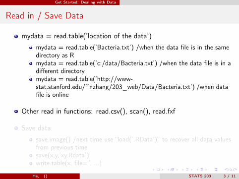
mydata = read.table(’location of the data’)
mydata = read.table(’Bacteria.txt’) /when the data file is in the samedirectory as Rmydata = read.table(’c:/data/Bacteria.txt’) /when the data file is in adifferent directorymydata = read.table(’http://www-stat.stanford.edu/~nzhang/203_web/Data/Bacteria.txt’) /when datafile is online
Other read in functions: read.csv(), scan(), read.fxf
Save data
save.image() /next time use “load(’.RData’)” to recover all data valuesfrom previous timesave(x,y,’xy.Rdata’)write.table(x, file=”, ...)
He, () STATS 203 3 / 11
Get Started: Dealing with Data
Read in / Save Data
mydata = read.table(’location of the data’)
mydata = read.table(’Bacteria.txt’) /when the data file is in the samedirectory as Rmydata = read.table(’c:/data/Bacteria.txt’) /when the data file is in adifferent directorymydata = read.table(’http://www-stat.stanford.edu/~nzhang/203_web/Data/Bacteria.txt’) /when datafile is online
Other read in functions: read.csv(), scan(), read.fxf
Save data
save.image() /next time use “load(’.RData’)” to recover all data valuesfrom previous timesave(x,y,’xy.Rdata’)write.table(x, file=”, ...)
He, () STATS 203 3 / 11
Get Started: Dealing with Data
“Data Structure”
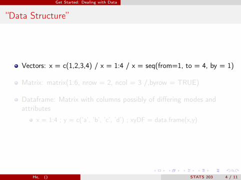
Vectors: x = c(1,2,3,4) / x = 1:4 / x = seq(from=1, to = 4, by = 1)
Matrix: matrix(1:6, nrow = 2, ncol = 3 /,byrow = TRUE)
Dataframe: Matrix with columns possibly of differing modes andattributes
x = 1:4 ; y = c(’a’, ’b’, ’c’, ’d’) ; xyDF = data.frame(x,y)
He, () STATS 203 4 / 11

Get Started: Dealing with Data
“Data Structure”
Vectors: x = c(1,2,3,4) / x = 1:4 / x = seq(from=1, to = 4, by = 1)
Matrix: matrix(1:6, nrow = 2, ncol = 3 /,byrow = TRUE)
Dataframe: Matrix with columns possibly of differing modes andattributes
x = 1:4 ; y = c(’a’, ’b’, ’c’, ’d’) ; xyDF = data.frame(x,y)
He, () STATS 203 4 / 11
Get Started: Dealing with Data
Operations on Data
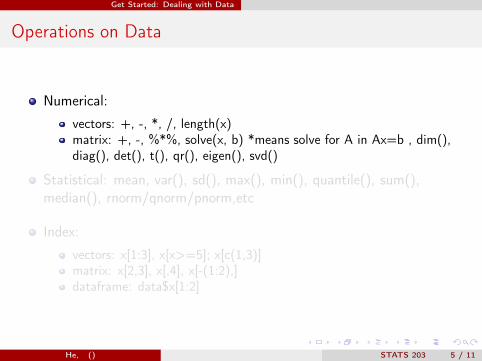
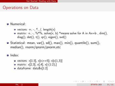
Numerical:
vectors: +, -, *, /, length(x)matrix: +, -, %*%, solve(x, b) *means solve for A in Ax=b , dim(),diag(), det(), t(), qr(), eigen(), svd()
Statistical: mean, var(), sd(), max(), min(), quantile(), sum(),median(), rnorm/qnorm/pnorm,etc
Index:
vectors: x[1:3], x[x>=5]; x[c(1,3)]matrix: x[2,3], x[,4], x[-(1:2),]dataframe: data$x[1:2]
He, () STATS 203 5 / 11

Get Started: Dealing with Data
Operations on Data
Numerical:
vectors: +, -, *, /, length(x)matrix: +, -, %*%, solve(x, b) *means solve for A in Ax=b , dim(),diag(), det(), t(), qr(), eigen(), svd()
Statistical: mean, var(), sd(), max(), min(), quantile(), sum(),median(), rnorm/qnorm/pnorm,etc
Index:
vectors: x[1:3], x[x>=5]; x[c(1,3)]matrix: x[2,3], x[,4], x[-(1:2),]dataframe: data$x[1:2]
He, () STATS 203 5 / 11
Higher Level
Control Structure
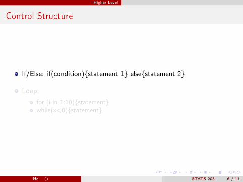
If/Else: if(condition){statement 1} else{statement 2}
Loop:
for (i in 1:10){statement}while(x<0){statement}
He, () STATS 203 6 / 11
Higher Level
Control Structure
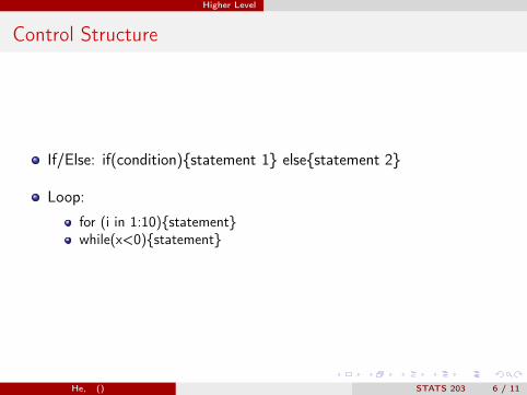
If/Else: if(condition){statement 1} else{statement 2}
Loop:
for (i in 1:10){statement}while(x<0){statement}
He, () STATS 203 6 / 11
Higher Level
Function
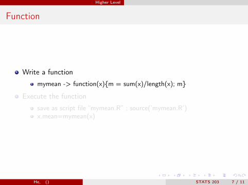
Write a function
mymean -> function(x){m = sum(x)/length(x); m}
Execute the function
save as script file “mymean.R” ; source(’mymean.R’)x.mean=mymean(x)
He, () STATS 203 7 / 11

Higher Level
Function
Write a function
mymean -> function(x){m = sum(x)/length(x); m}
Execute the function
save as script file “mymean.R” ; source(’mymean.R’)x.mean=mymean(x)
He, () STATS 203 7 / 11

Higher Level
Graphics
Ploting functions
plot(x), plot(x,y), boxplot(x), hist(x), qqplot(x,y), image (x,y,z)points(x,y), lines(x,y), abline(a,b), title()parameters: type, xlim/ylim, xlab/ylab, main, etc
He, () STATS 203 8 / 11
Higher Level
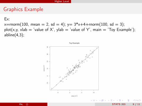
Graphics Example
Ex:x=rnorm(100, mean = 2, sd = 4); y= 3*x+4+rnorm(100, sd = 3);plot(x,y, xlab = ’value of X’, ylab = ’value of Y’, main = ’Toy Example’);abline(4,3);
He, () STATS 203 9 / 11

Higher Level
Statistical Analysis
Regression:
tmp = lm(y~x1+x2) model:y = β0 + β1x1 + β2x2 + εsummary(tmp); tmp$coefficients, tmp$residuals, tmp$fitted.values
Regression formulae
remove the constant term: tmp1 = lm(y~x-1) model: y = ax + εinteraction term: tmp = lm(y~x1:x2) model: y = βx1x2 + εfull model: tmp = lm(y~x1*x2) model:y = β0 + β1x1 + β2x2 + β3x1x2 + ε
He, () STATS 203 10 / 11

Reference
Reference
R tutorial by Yuehwen Liao last year
http://cran.r-project.org/
Have a problem?
google R and Function Name?(function name)?.search(function name)
He, () STATS 203 11 / 11