r tutorial 2013-08-20 - uga stratigraphy labstrata.uga.edu/software/pdf/rtutorial.pdf · a short r...

A SHORT R TUTORIAL

Steven M. HollandDepartment of Geology, University of Georgia, Athens, GA 30602-2501

�

13 September 2017

Installing RR is open-source and is freely available for macOS, Linux, and Windows. You can download compiled versions of R (called binaries, or precompiled binary distributions) by going to the home page for R (http://www.r-project.org), and following the link to CRAN (the Compre-hensive R Archive Network). You will be asked to select a mirror; pick one that is geographi-cally nearby. On the CRAN site, each operating system has a FAQ page and there is also a more general FAQ. Both are worth reading.

To download R, macOS users should follow the macOS link from the CRAN page and select the file corresponding to the most recent version of R. This will download a disk image with a file, which you should double-click to install R. R can be run from the apps R and RStudio, from the command line in Terminal.app, or from the command line in X11.

Linux users should follow the links for their distribution and version of Linux and download the most recent version of R. There is a read-me file that explains the download and installa-tion process.

Windows users should follow the link for Windows and then the link for the base package. A read-me file contains the installation instructions.

For more details, follow the Manuals link on the left side of the R home page. R Installation and Administration gives detailed instructions for installation on all operating systems.

Although most users will not want to do this, if you have special needs and want to compile the R source code yourself, you can also download it from the CRAN site.

In addition to R, you should install a good text editor. For macOS, BBEdit and TextWrangler are excellent text editors; both are available from Bare Bones Software. For Windows, Notepad++ is highly recommended, and it is free. I do not recommend using a word processor (like Word) instead of a good text editor.

Learning RThere are an enormous number of books on R. Several I’ve read are listed below, from the more basic to the more advanced. The R Book is my favorite, and The Art of R Pro-gramming is essential if you have a programming background or get serious about pro-gramming in R.

Statistics : An Introduction using R, by Michael J. Crawley, 2014. John Wiley & Sons, 360 p. ISBN-13: 978-1118941096. Amazon Price: $31.06

Using R for Introductory Statistics, by John Verzani, 2014. Chapman & Hall/CRC, 518 p. ISBN-13: 978-1466590731. Amazon Price: $40.14

The R Book, by Michael J. Crawley, 2012. Wiley, 1076 p. ISBN-13: 978-0470973929. Amazon Price: $70.13

A Short R Tutorial �1

An R and S-Plus® Companion to Multivariate Analysis, by Brian S. Everitt, 2007. Springer, 221 p. ISBN-13: 978-1852338824. Amazon Price: $62.52

Data Analysis and Graphics Using R, by John Maindonald, 2010. Cambridge Univer-sity Press, 549 p. ISBN-13: 978-0521762939. Amazon Price: $84.63

Ecological Models and Data in R, by Benjamin M. Bolker , 2008. Princeton Universi-ty Press, 408 p. ISBN-13: 978-0691125220. Amazon Price: $51.31

The Art of R Programming: A Tour of Statistical Software Design, by Norman Matloff, 2011. No Starch Press, 400 p. ISBN-13: 978-1593273842. Amazon Price: $24.56

The manuals link on the R home page has links to three important guides. The Introduction to R is highly recommended as a basic source of information on R. R Data Import/Export is useful for understanding the many ways in which data may be imported into or exported from R. The R Reference Index is a gigantic pdf (3500 pages!) that comprehensively lists all help files in a standard R installation. These help files also freely accessible in every installation of R.

Everyone likely has their favorite web sites for R, and these three are mine.

R -bloggers (http://www.r-bloggers.com) is a good news and tutorial site that aggregates from over 750 contributors. Following its RSS feed is a good way to stay on top of what’s new and to discover new tips and analyses.

Cookbook for R (http://www.cookbook-r.com) has recipes for analyzing your data.

Stack Overflow (http://stackoverflow.com/questions/tagged/r) is a question and answer site for programmers. Users post questions, other users post answers, and these get voted up or down, so you can see what the community regards as the right answer. Stack Overflow is great for many languages, and the R community that uses it is growing.

Finally, remember when you run into a problem that Google is your friend.

Objects and FunctionsWhen you launch R, you will be greeted with a prompt (>) and a blinking cursor:

>

For every command in this tutorial, I will show the prompt, but you should not type it.

R works with objects, and there are many types. Objects store data, and they have commands that can operate on them, which depend the type and structure of data that is stored. A single number or string of text is the simplest object and is known as a scalar. [Note that a scalar in R is simply a vector of length one; there is no distinct object type for a scalar, although that is not critical for what follows.]


To give a value to an object use one of the two assignment operators. Although the equals sign may be more familiar, the arrow (less-than sign, followed by a dash: <-) is more common, and you should use it.

> x = 3 > x <- 3

To display the value of any object, type its name at the prompt.

> x

Arithmetic operators follow standard symbols for addition, subtraction, multiplication, divi-sion, and exponents:

> x <- 3 + 4 > x <- 2 - 9 > x <- 12 * 8 > x <- 16 / 4 > x <- 2 ^ 3

Comments are always preceded by a pound sign (#), and what follows the pound sign on that line will not be executed.

> # x <- 2 * 5; everything on this line is a comment > x <- 2 * 5 # comments can be placed after a statement

Spaces are generally ignored, but include them to make code easier to read. Both of these lines produce the same result.

> x<-3+7/14 > x <- 3 + 7 / 14

Capitalization generally matters, as R is case-sensitive. This is especially important when call-ing functions, discussed below.

> x <- 3 > x # correctly displays 3 > X # produces an error, as X doesn’t exist, but x does

Because capitalization matters, you should avoid giving objects names that differ only in their capitalization, and you should use capitalization consistently. One common pattern is camel-case, in which the first letter is lower case, but subsequent words are capitalized (for example, pacificOceanData). Another common pattern is to separate words in an object’s name with a period (pacific.ocean.data). More rarely, some separate words in an object’s name with an underscore (pacific_ocean_data). Pick one and be consistent.

You can use the up and down arrows to reuse old commands without retyping them. The up arrow lets you access progressively older previously typed commands. If you go too far, use the down arrow to return to more recent commands. These commands can be edited, so the up and down arrows are good time-savers, even if you don’t need to use exactly the same command as before.


FunctionsR has a rich set of functions, which are called with any arguments in parentheses and which generally return a value. Functions are also objects. The maximum of two values is calculated with the max() function:

> max(9, 5) > max(x, 4) # objects can be arguments to functions

Some functions need no arguments, but the parentheses must still be included, otherwise R will interpret what you type as the name of a non-function object, like a vector or matrix. For example, the function objects(), which is used to display all R objects you have created, does not require any arguments and is called like this:

> objects() # correct > objects # error

Neglecting the parentheses means that you are asking R to display the value of an object called objects, which likely doesn’t exist.

Functions usually return a value. If the function is called without an assignment, then the re-turned value will be displayed on the screen. If an assignment is made, the value will be as-signed to that object, but not displayed on the screen.

> max(9, 5) # displays 9 > myMax <- max(9, 5) # stores 9 in myMax

Multiple functions can be called in a single line, and functions can be nested, so that the re-sult of one function can be used as an argument for another function. Nesting functions too deeply can make the command long, confusing, and hard to debug if something should go wrong.

> y <- (log(x) + exp(x * cos(x))) / sqrt(cos(x) / exp(x))

To get help with any function, use the help() function or the ? operator, along with the name of the function.

> help(max) > ?max > ? max

The help pages show useful options for a function, plus background on how the function works, references to the primary literature, and examples that illustrate how the function could be used. Use the help pages.

In time, you will write your own functions because they allow you to invoke multiple com-mands with a single command. To illustrate how a simple function is created and used, con-sider the pow() function shown below, which raises a base to an exponent. In parentheses after the word function is a list of parameters to the function, that is, values that must be input into the function. When you call a function, you supply arguments (values) for these pa-


rameters. The commands the function performs are enclosed in curly braces. Indenting these statements is not required, but it makes the function easier to read.

> pow <- function(base, exponent) { result <- base^exponent result }

Arguments can be assigned to a function’s parameters in two ways, by name and by position. When you assign arguments by name, they can be listed in any order and the function will give the same result:

> pow(base=3, exponent=2) # returns 9 > pow(exponent=2, base=3) # also returns 9

Assigning arguments by position saves typing by omitting the parameter names, but the ar-guments must in the correct order.

> pow(3, 2) # returns 3^2, or 9 > pow(2, 3) # returns 2^3, or 8

For pow(), the first position is assumed to hold the first parameter in the function definition (base) and the second position is assumed to hold the second parameter (exponent).

Some functions have default values for some parameters. For example, pow() could be writ-ten as

> pow <- function(base, exponent=2) { result <- base^exponent result }

which makes the default exponent equal to 2. If you write pow(2), you’ll get 4 in return (2 to the second power). If you want a different exponent, specify the exponent argument, such as pow(2, 5), which would produce 32 (2 to the fifth power). Refer to a function’s help page to see which function parameters have default assignments.

Several functions are useful for manipulating objects in R. To show all current objects, use objects() and ls().

> objects() > ls() # either works

To remove objects, use remove(). Removing an object is permanent; it cannot be undone.

> remove(someObject)

You can also remove all objects, but since this cannot be undone, be sure that this is what you want to do. Even if you remove all objects, your command history is preserved, so you could reconstruct your objects, although this might be laborious. There is no single command for


removing all objects. To do this, you must combine two commands, the ls() function and the remove() function.

> remove(list=ls())

VectorsA vector is a series of values, which may be numeric or text, where all values have the same type, such as integers, decimal numbers, complex numbers, characters (strings), and logical (Boolean). Vectors are common data structures, and you will use them frequently. Vectors are created most easily with the c() function (c as in concatenate). Short vectors are easily entered this way, but long ones are more easily imported (see below).

> x <- c(3, 7, -8, 10, 15, -9, 8, 2, -5, 7, 8, 9, -2, -4, -1)

An element of a vector can be retrieved by using an index, which describes its position in the vector, starting with 1 for the first element. To see the first element of x, type:

> x[1] # returns 3

Multiple consecutive indices can be specified with a colon. For example, to retrieve elements 3 through 10, type

> x[3:10] # returns -8, 10, 15, -9, 8, 2, -5, 7

To retrieve non-consecutive elements, use the c() function. Failing to use c()will cause an error.

> x[c(1, 3, 5, 7)] # returns 3, -8, 15, 8

These two approaches can be combined in more complex ways. For example, if you wanted elements 3 through 7, followed by elements 5 through 9, you would type:

> x[c(3:7, 5:9)] # returns a vector with -8, 10, 15, -9, 8, 15, -9, 8, 2, -5

You can use conditional logic to select elements meeting certain criteria. The logical state-ment inside the bracket produces a vector of boolean values (TRUE and FALSE), which tell whether a particular vector element should be returned.

> x[x>0] # all positive values in x > x[x<=2] # values less than or equal to 2 > x[x==2] # all values equal to 2 > x[x!=2] # all values not equal to 2 > x[x>0 & x<3] # values greater than 0 and less than 3 > x[x>5 | x<1] # values greater than 1 or less than 1

Any Boolean vector can be negated with the ! operator, but this is often overlooked when reading code, and it is often better to use other operators that are more direct, such as !=.


Vectors can be sorted with the sort() function. Ascending order is the default.

> sort(x)

Sorting can be done in descending order by specifying decreasing = TRUE or by revers-ing the sorted vector with rev(). The first way is preferred.

> sort(x, decreasing=TRUE) > rev(sort(x))

R speeds calculations by using what is called vectorized math. For example, suppose you wanted to multiply all values in a vector by a constant. If you have programmed before, you might think of doing this with a loop, in which you step through each value in a vector and multiply it by a constant. Avoid doing this in R, as loops are slow, so much so that they won’t be presented until near the end of this tutorial). Instead, simply multiply the vector by the constant in one line. This example multiplies all of the values in a vector by 2.

> x <- c(1, 3, 5, 7, 9) > y <- 2 * x

Likewise, you can use vector arithmetic on two vectors. For example, given two vectors of the same length, it is easy to add the first element of the one vector to the second element of the second vector and so on, producing a third vector of the same length with all of the sums.

> x <- c(1, 3, 5, 7, 9) > y <- c(2, 2, 2, 4, 4) > z <- x + y

FactorsFactors are similar to vectors, but they have a fixed number of levels and are ideal for express-ing categorical variables. For example, if had a series of sites, each representing a habitat type, store them as a factor rather than as a vector:

> x <- factor('marsh', 'grassland', 'forest', 'tundra', 'grassland', 'tundra', 'forest', 'marsh', 'grassland')

Inspecting the objects shows that it is stored differently than a vector.

> x [1] marsh grassland forest tundra grassland tundra [7] forest marsh grassland Levels: forest grassland marsh tundra

We can use the str() function to display its internal structure:

> str(x) Factor w/ 4 levels "forest","grassland",..: 3 2 1 4 2 4 1 3 2


Although the names are displayed when we show the object, the data are actually saved as values 1–4, with each value corresponding to a named factor. For example, the first element is saved as a 3, that is, the third level of the factor (marsh). The second element is saved as a 2, the second level of the factor (grassland), and so on. This is not only a more compact way of saving the data, it also allows efficient ways to use these categories, such as using tapply()and by() to perform calculations on each category, split() to separate the data by category, and table() to create tables of the data by category.

If needed, a factor can always be converted to a vector:

> y <- as.vector(x)

ListsLists are another type of data structure, one closely related to vectors. Lists hold a series of values, like vectors, but the values in a list can be of different types, unlike a vector. For exam-ple, the first element of a list might be a string giving the name of a locality ('Hueston Woods'), the second element might be an integer expressing the number of beetle species found (42), and the third element might be a boolean value stating whether the locality is old-growth forest (TRUE). Lists are made with the list() function:

> x <- list('Hueston Woods', 42, TRUE)

Lists are commonly produced by statistical functions, such as regressions or ordinations.

To access an element of a list, use double brackets instead of single brackets.

> x[[1]] # returns 'Hueston Woods'

Elements in a list are often labelled, and when they are, they can be accessed by their name. For example, when you perform a linear regression, a linear regression lm object is returned, and it is a list that contains twelve items, including the slope, the intercept, confidence limits, p-values, residuals, etc. If you ran a regression and assigned the result to forestRegres-sion, you could find the names of all the elements in the forestRegression list with the names() function.

> names(forestRegression)

One of the elements of the list is called residuals, and you can use dollar-sign notation to ac-cess it by name:

> forestRegression$residuals

Because residuals is the second element in the list, you could also access it by position with the double-brackets notation:

> forestRegression[[2]]


Because these residuals are a vector, you can access individual elements of the vector by adding brackets. For example, you could get the residual for the third data point in two ways:

> forestRegression$residuals[3] # method 1 > regressionResults[[2]][3] # method 2

MatricesAnother type of R data structure is a matrix, which has multiple rows and columns of values, all of the same type, like a vector. You can think of a matrix as a collection of vectors, all of the same type.

Small matrices can be entered easily with the matrix() function, in which you specify the data as a vector and the number of rows or columns.

> x <- matrix(c(3, 1, 4, 2, 5, 8), nrow=3)

This will generate a matrix of 3 rows and therefore 2 columns, since there are six elements in the matrix. By default, the matrix is filled by columns, such that column 1 is filled first from top to bottom, then column 2, etc. Thus, the x matrix would be:

3 2 1 5 4 8

The matrix can be filled by rows instead, with row 1 filled first, from left to right, then row 2, etc., by including the argument byrow=TRUE:

> x <- matrix(c(3,1,4,2,5,8), nrow=3, byrow=TRUE)

This gives

3 1 4 2 5 8

Large matrices can also be entered this way, but importing them is easier (see Importing Larger Data Sets below).

Matrices also use vectorized math, greatly speeding computation.

Data FramesA data frame is like a matrix, but the columns can be of different types. For example, one col-umn might be locality names (strings), several others might be counts of different species of beetles (integers), and others might be Boolean values that describe properties of the locali-ties, such as whether it is old-growth forest. In this way vectors are to lists as matrices are to data frames.


Nearly always, columns of a matrix or data frame should be the measured variables, and the rows should be cases (localities, samples, etc.). If you have a dataset in which these are re-versed, you can swap columns for rows and vice versa (transpose the matrix), with the t() function:

> y <- t(x)

Retrieving elements of a matrix and data frame follows a similar approach, in which square brackets surround two or more indices corresponding to the dimensions of the matrix. For a two-dimensional matrix or data frame, the square brackets would contain two indices, sepa-rated by a comma. The first index is the row number, and the second is the column.

> y[3, 5] # third row, fifth column

Like lists, columns (variables) in data frames can have names. To find the names of the col-umns, use the colnames() function.

> colnames(y)

Column names can also be assigned:

> colnames(y) <- c('locality', ‘beetle1', 'beetle2', 'beetle3', ‘beetle4', ‘oldGrowth')

Individual columns can be accessed with the $ operator. For example, this will return the col-umn named beetle1 from the y data frame.

> y$beetle1

Dollar-sign notation will not work for selecting multiple columns. To select multiple columns, use their column number; leaving the row position empty will select all the rows for the col-umn. The following returns all the rows for columns 2 through 5 of the y data frame.

> y[ ,2:5]

To access individual elements (cases) of such a data vector, add brackets with indices. Both of the following return the first four values (rows) of beetle1, which is in column 2 of the y data frame.

> y$beetle1[1:4] > y[1:4, 2]

If the name of the data frame is long, $ notation can become cumbersome. To avoid repeated-ly typing the name of the data frame, you can use the attach() function, which creates copies of all the variables (columns) in the data frame that can be directly accessed. The de-tach() function deletes these copies.

> attach(y) > Fe # Fe can be accessed without $ notation > detach(y) > Fe # returns an error - detach() destroyed the copy


Because attach() creates copies, changes made to the attached data are not be saved in the original data frame.

The attach() and detach() commands also work on lists.

A danger in using attach() is that it may mask existing variables with the same name, mak-ing it unclear which version is being used. attach() is best used when you are working with a single data frame. If you must use it in more complicated situations, be alert for warnings about masked variables, and call detach()as soon as possible. There are alternatives to at-tach(), including the data parameter in some functions (such as regressions) that lets you access variables of data frame directly, as well as the with() function, another safe alterna-tive that can be used in many situations.

Sorting a matrix or data frame is more complicated than sorting a vector. It is often best to store the sorted matrix or data frame in another object in case something is typed wrong. The following sorts the data frame A by the values in column 3 and stores the result in data frame B.

> B <- A[order(A[ ,3]), ]

To understand how this complex command or any complex command works, take it apart, starting at the innermost set of parentheses and brackets, and work outwards. Starting at the inside, A[ ,3] returns all rows of column 3 from matrix A. Stepping out one level, order(A[ ,3]) returns the order number of the elements in that column as if they were sorted in ascending order. In other words, the smallest value in column 3 would have a value of 1, the next smallest would have a value of 2, and so on. Finally, these values specify the de-sired order of the rows in the A matrix, and A[order(A[ ,3]), ] returns all the columns with the rows in that order.

This technique of taking apart a complex function call is known as unpacking. You should do this whenever a complex function call returns unexpected results or when you need to under-stand a complex function call works.

Finally, your data may be in a matrix, but R may require it to be in a data frame for some func-tion (or vice versa). You can try to coerce it into the correct type with the functions as.da-ta.frame() and as.matrix().

ydf <- as.data.frame(y) z <- as.matrix(ydf)

If you need to find the type of an object, use the class() function.

> class(y) # returns "matrix" > class(ydf) # returns "data.frame" > class(z) # returns "matrix"


Importing Larger Data SetsFor larger data sets, it is generally easier to enter the data in a spreadsheet (like Excel), check it for errors, and then export the file into a format you can read into R. The most widely used file formats are comma-delimited and tab-delimited text. In Excel, choose Save As..., then select “Comma-separated values (.csv)” or “Tab-delimited text (.txt)”. Both are text-only for-mats that can be read by almost any application.

To preserve the readability of your data for many years, always save a copy of your data in a text-only format. Binary file formats for programs like Excel do change over time, and the result is that you may someday not be able to read your old files. This will not happen with plain text files.

To read or write files in R, you need to know the current working directory for R, which can be found with the getwd()function:

> getwd()

It is easiest to work with R by using a single working directory for any given session, and you can set this with the setwd() function. This directory will hold most or all of the files you will need to read, such as data or source code, and it will be where files are saved to by default. R will stay in this working directory unless you specify a different path to a file.

Because the UNIX (macOS, Linux) file systems differ from that of Windows, paths are speci-fied differently. This is one of the few areas in which R works differently on the two plat-forms. Bear in mind that if you share code across platforms, any command that accesses the file system will produce an error, so it is best to set any directory in a single, obvious place in your code, such as in the first line of your file of commands.

Use the setwd() function to set the working directory of R, with the path as an argument. Because the path is a string, you must wrap it in quotes, and this is true for any string in R. Single-quotes and double-quotes both work; just be consistent. Single quotes are preferred because they are faster to type. Inside the path, use single forward slashes for UNIX systems, but remember to use double back-slashes for Windows.

> setwd('/Users/myUserName/Documents/Rdata') # UNIX (macOS and Linux)

> setwd('C:\\Documents and Settings\\myUserName\\Desktop') # Windows

Once you’ve set your working directory, you can read a vector into R with the scan() func-tion. Remember to put your file name in quotes, and include the suffix.

> myData <- scan(file='myDataFile.txt')

If you want to access a file that is not in your current directory, include the path with the file name:


> myData <- scan(file='/Users/myUserName/Documents/myDataFile.txt') # UNIX systems (Linux, macOS)

> myData <- (file='C:\\SomeDirectory\\myDataFile.txt') # Windows

Note that embedding paths like this is likely to cause an error if others use your code, so it is best to avoid it, unless you have taken precautions to ensure that the path always exists.

To read a table of values into R and save it as a data frame, use the read.table() function. This function assumes that your data are in the correct format, with columns corresponding to variables and rows corresponding to samples. All cells should contain a value; don’t leave any empty. If a value is missing, enter NA in that cell. Variable names can be as long as you need them to be. Variable names do not need to be single words, but any blank spaces will be replaced with a period when you import the data into R.

Of the many options for read.table(), you will primarily pay close attention to three things, which you can determine by examining the data file in a text editor. First, check to see if there are column names for the variables, that is, whether a header is present. Second, check to see if there are row names and what column they are in (conventionally the first column). Third, check to see what separates the columns; tabs or commas are the most common separa-tors, also called delimiters.

For example, suppose that your data table has the names of its variables in its first row (a header), that your samples names are in the first column of the table, and that your values are separated by commas. Given this, you would import your data as follows:

> myData <- read.table(file='myDataFile.txt', header=TRUE, row.names=1, sep=',')

If there is no header, leave out the argument for the header parameter, because the default is that a header will be absent. Likewise, if there are no row names, leave out the argument for the row.names parameter. If the values are separated by tabs, use sep=‘\t’. There are other commands like read.csv(), but you should become comfortable opening any table file with read.table(); it is the Swiss-army knife of file openers.

When you read in a data file, it is wise to verify that it was read correctly. Although the im-pulse is to type the name of the object under which it is save, this can produce an unnecessar-ily voluminous output. It is better to use the head() and tail() functions to examine the first few lines of data and the last few lines.

> head(myData) > tail(myData)


Generating NumbersWriting long, regular sequences of numbers is tedious and error-prone. R can generate these quickly with the seq() function. If the increment (by) isn’t set, it defaults to 1.

> seq(from=1, to=100) # integers from 1 to 100 > seq(from=1, to=100, by=2) # odd numbers from 1 to 100 > seq(from=0, to=100, by=5) # counting by fives

R can easily generate random numbers from many statistical distributions. A few common examples include runif() for uniform or flat distributions, rnorm() for normal distribu-tions, and rexp() for exponential distributions. For each, specify the number of random numbers (n) and one or more parameters that describe the distribution. For example, this generates 10 random numbers from a uniform distribution that starts at 1 and ends at 6:

> runif(n=10, min=1, max=6)

This creates ten random numbers from a normal distribution with a mean of 5.2 and a stan-dard deviation of 0.7:

> rnorm(n=10, mean=5.2, sd=0.7)

This produces ten random numbers from an exponential distribution with a rate parameter of 7:

> rexp(n=10, rate=7)

Basic StatisticsR has functions for calculating simple descriptive statistics from a vector of data, such as:

> mean(x) # arithmetic mean > median(x) # middle value > length(x) # number of elements in x (sample size) > range(x) # largest and smallest value > sd(x) # standard deviation > var(x) # variance

Many statistical tests are built-in. Some of the most common include:

> t.test(x, y) # t-test for equality of means > var.test(x, y) # F-test for equality of variance > cor(x, y) # correlation coefficient > lm(y~x) # least squares regression > anova(lm(x~y)) # ANOVA (analysis of variance) > wilcox.test (x, mu=183) # Mann-Whitney U test > kruskal.test(x~y) # Non-parametric ANOVA > ks.test(x, y) # Kolmogorov-Smirnov test


In addition to generating random numbers, the built-in statistical distributions of R can be used to find probabilities or p-values, find critical values, or draw probability density func-tions. These commands are set up consistently, although their parameters may differ. For ex-ample, these can be performed with the normal distribution through the pnorm(), qnorm(), and dnorm() functions.

The pnorm() function will find the area under a standard normal curve, starting from the left tail, and in the example below, going to a value of 1.96. Note that 1 minus this value would correspond to the p-value for a Z-test, where Z=1.96:

> pnorm(q=1.96)

The qnorm() function can find the critical value for a given probability. For example, in a two-tailed test at a significance level of 0.05, the following gives the critical value on the right tail.

> qnorm(p=0.975)

Last, the dnorm() function gives the density or height of the distribution at a particular val-ue (at 1.5 below). By doing this over all values, you could plot the shape of the distribution.

> dnorm(x=1.5)

Other distributions, such as the uniform, exponential, and binomial distributions follow a similar syntax.

> rbinom(n=10, size=15, prob=0.1) # binomial distribution > pexp(q=7.2) # exponential distribution > qunif(p=0.95) # uniform distribution

One of the great strengths of R is the incredibly large number of available statistical analyses. Many are built into the base package of R, but an ever-growing number of them are freely available in user-contributed packages. There’s a good chance that if you need to do an analy-sis, it is already available in R.

Efficient computationR has vectorized math, which eliminates the need for looping through vectors and matrices to perform many calculations. Such vectorized calculations are commonly orders of magnitude faster than using loops.

Another set of tools for efficient computation are the apply() family set of functions. The most basic of these is apply(), which is useful when you want to perform a function on every row or every column of a matrix or data frame and get the results as a vector. For exam-ple, the following calculates the median for every column of the matrix and returns a vector with those medians.

medians <- apply(x, MARGIN=2, FUN=median)


Set MARGIN to 1 to calculate the median for every row instead. The argument to FUN is the name of the function to be applied, and it could be a function that you create.

The functions sapply() and lapply() are similar, but it when a function needs to be ap-plied to all elements of a vector or a list. lapply() returns a list, but sapply() can return the results as a vector or matrix. One possible use of both would be to have a series of similar data sets stored as elements of a list, then call lapply() or sapply() once to perform a function on each of the data sets. This would be simpler than looping through the list and performing the calculations separately on each data set, and far superior to storing the data sets as separate objects and performing the calculations separately on each object. By creating your own function as a wrapper around other functions, you could perform a complex series of analyses, including making and saving plots for each data set, all in one command.

PlotsAnother strength of R is the quality of its plotting routines. Many types of plots are available, and complex plots can be produced. R’s plots are far superior to those made in spreadsheets like Excel.

When calling an R plotting function, the plot will automatically be generated in the active plotting window, if one already exists. If no plot window exists, a new one will be created with the default settings. Use dev.new() to create a new plot window, as this command will work on any platform. Avoid using the platform-specific ways of creating new plot windows, such as quartz()for macOS, X11() for Linux, and windows() for Windows, because these will generate errors if your code is run on a different platform. Always write your code in a way that will make it portable.

The height and width in inches of a plot window can be specified, or they can be left off for the default window.

> dev.new(height=7, width=12) # custom size, in inches > dev.new() # default size

H I S T O G R A M S

Histograms or frequency distributions are generated with the hist() function, which can be controlled in various ways. Calling hist() with no additional arguments generates a default histogram.

> hist(x)

Histograms can be customized by changing the number of bars or divisions with the breaks parameter. Oddly for R, this is only a suggestion that may not be honored.

> hist(x, breaks=20)

The divisions in the histogram can be forced by specifying their locations as a vector.


> divisions <- c(-2.5, -2, -1, 0, 1, 1.5, 2, 2.5) > hist(x, breaks=divisions)

S C A T T E R P L O T S

Scatterplots (x-y plots) are generated with the plot() function. The first argument corre-sponds to the horizontal axis, and the second is shown on the vertical axis.

> plot(x, y)

Labels for the x and y axes can be set with the xlab and ylab parameters, and the plot title can be set with the main parameter. Remember to put strings in quotes.

> plot(x, y, main='Iron contamination at mine site', xlab='pH', ylab='Fe content')

The pch parameter can be set in plot() to specify a particular type of symbol. The value of 16 is a filled circle, an easily visible symbol that you should use.

> plot(x, y, pch=16)

Twenty-five plotting symbols are available in pch:

By changing the argument to the type parameter, you can control whether lines or points are plotted.

> plot(x, y, type='p') # points only > plot(x, y, type='l') # connecting lines only, no points > plot(x, y, type='b') # both points and lines > plot(x, y, type='n') # no points, only axes and labels

Symbol colors can be set with the col parameter. To see the full list of 657 named colors in R, use the colors() function. Colors can also be specified by RGB (red-green-blue) value, if you are familiar with creating colors for web pages.

> plot(x, y, pch=16, col='green') # small green filled circles > colors() # lists all named colors > plot(x, y, col='#00CCFF') # 00CCFF is pale blue

Equations and special symbols can be used in figure labels and as text added to figures. See the help page for plotmath() for more details. The function text() is used for placing


additional text onto a figure, expression() creates an object of type “expression”, and paste() is used to concatenate items. The help pages for these functions are useful for see-ing the basic ways for combining these useful functions. The first example puts the square root of x as the y-axis label, and the second example shows the standard symbol for the oxy-gen isotope ratio on the y-axis.

> plot(x, y, ylab=expression(paste(sqrt(x)))) > plot(x, y, ylab=expression(paste(delta^18, 'O')))

A D D I N G T O P L O T S

Text annotations can be added with the text() function, where the x and y arguments de-scribe the position of the annotation, and labels specifies what text will be added. The x and y coordinates are identical to those used for placing points on the plot.

> text(x=10, y=2, labels=expression(sqrt(x)))

Lines can be added to a plot with the abline() function. You can make horizontal and ver-tical lines, as well as lines with a specified slope and intercept.

> abline(h=5) # horizontal line at a y=5 > abline(v=10) # vertical line at a x=10 > abline(a=intercept, b=slope) # line with slope and intercept > abline(lm(y~x)) # line fitted by a regression

Shapes can also be added to the plot, and these can be customized with particular line types (dashed, dotted, etc.), colors of lines, and colors of fills. See lty in par() for customizing line types. Study the help page for par(), because it describes the many ways that plots can be customized.

The rect() function draws a box with the coordinates of the left, bottom, right, and top edges.

> rect(xleft=2, ybottom=5, xright=3, ytop=7)

The arrows() function draws an arrow, with the first two parameters specifying the x and y coordinate of the origin of the line, and the third and fourth parameters specifying the coor-dinates of the arrowhead tip.

> arrows(x0=1, y0=1, x1=3, y1=4)

The segments() function is identical to the arrows() function, except that no arrow-head is drawn.

> segments(x0=1, y0=1, x1=3, y1=4)

Similarly, lines connecting data points can be added with lines(), and polygons can be added with and polygon(). A box can be drawn around the entire plot with box().


B U I L D I N G A C O M P L E X P L O T

Complex plots are typically built in stages, with groups of points added sequentially, and with custom axes, text, and graphic annotations added separately. To build a plot in stages, set type='n' to prevent data points from being plotted, and set axes=FALSE to prevent the axes from being drawn. Specify the values to be plotted along the x and y axes as the first two arguments.

> plot(x, y, type='n', axes=FALSE)

Points can be added to the current plot with the points() function. Only those points that are visible within the current limits of the axes will be shown. The limits of the axes are based on the values used in the data supplied to the plot() function.

> points(x, y)

Axes can be added individually with the axis() function.

> axis(1, at=seq(-1.0, 2.0, by=0.5), labels=c('-1.0', '-0.5', '0.0', '0.5', '1.0', '1.5', '2.0'))

The initial argument specifies the axis to be drawn, with 1 indicating the x axis and 2 indicat-ing the y-axis. The at parameter specifies where the tick marks should be drawn, and the labels parameter specifies the label to be displayed next to each tick mark. Note that the values given to labels are in quotes, as they are strings.

Here is an example of building a complex plot in parts. The commands that are shown were preceded by a good bit of experimentation (not shown) with different parts of the plot to de-termine the order in which these commands would be given. The data are read in, and at-tach() is used to make the variables accessible without dollar-sign notation.

> waves <- read.table(file='waves2.txt', header=TRUE, sep=',') > attach(waves)

Plotting begins by making a window with an aspect ratio appropriate for the data being plot-ted. This is a time series, so we would like the plot to be relatively wide to emphasize the changes over time.

> dev.new(height=4, width=10)

Because this is a scatterplot, the basic plot is built with the plot() command, specifying the x and y data as the first two arguments, the titles, the axis labels, and the limits of the y data range (ylim). The type is set to n, because the data will be added subsequently.

> plot(juliandate, SwH, main='Station 46042 - Monterey - 27 NM West of Monterey Bay, California', xlab='', ylab='Significant Wave Height (m)', axes=FALSE, type='n', ylim=c(0,6))


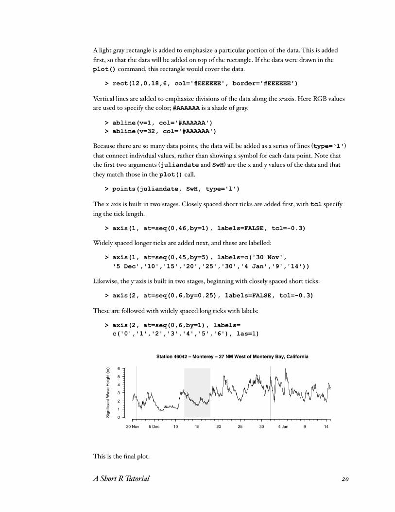
A light gray rectangle is added to emphasize a particular portion of the data. This is added first, so that the data will be added on top of the rectangle. If the data were drawn in the plot() command, this rectangle would cover the data.

> rect(12,0,18,6, col='#EEEEEE', border='#EEEEEE')

Vertical lines are added to emphasize divisions of the data along the x-axis. Here RGB values are used to specify the color; #AAAAAA is a shade of gray.

> abline(v=1, col='#AAAAAA') > abline(v=32, col='#AAAAAA')

Because there are so many data points, the data will be added as a series of lines (type=‘l') that connect individual values, rather than showing a symbol for each data point. Note that the first two arguments (juliandate and SwH) are the x and y values of the data and that they match those in the plot() call.

> points(juliandate, SwH, type='l')

The x-axis is built in two stages. Closely spaced short ticks are added first, with tcl specify-ing the tick length.

> axis(1, at=seq(0,46,by=1), labels=FALSE, tcl=-0.3)

Widely spaced longer ticks are added next, and these are labelled:

> axis(1, at=seq(0,45,by=5), labels=c('30 Nov', '5 Dec','10','15','20','25','30','4 Jan','9','14'))

Likewise, the y-axis is built in two stages, beginning with closely spaced short ticks:

> axis(2, at=seq(0,6,by=0.25), labels=FALSE, tcl=-0.3)

These are followed with widely spaced long ticks with labels:

> axis(2, at=seq(0,6,by=1), labels= c('0','1','2','3','4','5','6'), las=1)

This is the final plot.


Station 46042 − Monterey − 27 NM West of Monterey Bay, California

Sign

ifica

nt W

ave

Hei

ght (

m)

30 Nov 5 Dec 10 15 20 25 30 4 Jan 9 14

0

1

2

3

4

5

6

M U L T I P L E P L O T S O N A P A G E

Multiple plots can be drawn on the same page by using the par() function and setting the argument to mfrow. Each successive call to plot() will fill the panel from left to right, or from the top to the bottom, starting in the upper left corner.

> par(mfrow=(c(3, 2)))

This example will produce a page with areas for six plots in 3 rows and 2 columns. Each plot is added subsequently. Note that once one plot is finished and another plot is started, the first plot can no longer be modified.

Saving and Exporting Results

C O M M A N D S

From the R console window, you can copy and paste the entire R session into a text file. This will save a record of the commands you issued and the results that were displayed. This is an easy and simple way to save your work. Making a habit of this allows you to replicate your work, to build on it subsequently, and to apply your analyses to other data sets.

You can edit this text file so that it consists of just the commands you need. First, delete all the commands and their output that produced results you don’t want to keep. Next, delete all lines of results, leaving only lines of commands. Last, delete the > prompts at the beginning of each line, and any + marks at the beginnings of lines. If you copy and paste this code into a new R session, it should run without errors or warnings. If you get errors or warnings, edit the code and repeat this process until it runs clean. Save this file for a permanent record of your analysis.

P L O T S

On macOS, graphics produced in R can be saved as pdf files by selecting the window contain-ing the plot, and choosing Save or Save As from R's File menu. In Windows, graphics can be saved this way to metafile, postscript, pdf, png, bmp, and jpeg formats. I recommend saving plot files as pdfs because they can be edited in Adobe Illustrator. Other formats, particularly png, bmp, and jpeg should be avoided as they cannot be edited and because they often suffer from compression artifacts that can make them look fuzzy.

Graphics can also be built and saved to a file from the command line. Use the pdf() func-tion to open a pdf file, just as you would open a plotting window with dev.new(). Run all of your plotting commands, followed by dev.off() to close the pdf file. Note that your plot will not be displayed while you do this, although it is being written to a file.


> pdf(file='myPlot.pdf', height=7, width=7) > plot(x, y) # plus any other plotting commands > dev.off()

A typical strategy is to first develop a plot onscreen to refine the order of the plot commands. Once these are established, then open a pdf file with pdf(), rerun all of the plotting com-mands, and close the pdf file with dev.off().

O B J E C T S

Any objects generated in R, such as functions, vectors, lists, matrices, data frames, etc. can be saved to a file by using the command save.image(). Although this will not save any graph-ics, nor the command history, it is useful for saving the results of a series of analyses so they will not have to be regenerated in future R sessions. I recommend deleting unnecessary ob-jects before saving the image, particularly temporary or test objects generated when you were experimenting with code. If your work involves long-running computations to build an ob-ject, use save.image() so that it you don’t have to re-run those analyses the next time you work.

> save.image(file = 'myResults.RData')

When you resume your work, reload your objects with load(), allowing you to continue your analyses where you left off.

> load(file = 'myResults.RData')

Programming in RIf you have previous programming experience, get a copy of The Art of R Programming; it will save you much time. The most important programming advice I can give is to avoid loops, especially nested loops, which can dramatically slow your calculations.

Even so, some problems require loops.

R’s for loop is a generalized loop like the for loop in C or the do loop in FORTRAN. If you have programmed before, the syntax is intuitive and this will likely be the most common loop that you use. Note the use of curly braces if there is more than one statement inside the loop. There are various styles as to where the curly braces may be placed to help readability of the code, and they do not alter the execution. Indenting the code inside the loop helps to make the contents of the loop more apparent. Although indenting isn’t required, it is good form to do it.

Here is an example of calculating variance as you might in C or Fortran, that is, with loops

> x <- rnorm(10000000)

> sum <- 0 > for (i in 1:length(x)) sum <- sum + x[i]


> mean <- sum/length(x) # would be faster to use mean() > sumsquares <- 0 > for (i in 1:length(x)) { sumsquares <- sumsquares + (x[i]-mean)^2 } > variance <- sumsquares / (length(x)-1)

On a test computer, this ran in 16.3 seconds. If calculated variance with vectorized math,

> variance <- sum((x-mean)^2)/(length(x)-1)

it ran in a mere 0.23 seconds, a dramatic improvement. Using the built-in var() function, which has additional optimizations, it took only 0.082 seconds. If you test these times, you’ll likely get different numbers, but a similar improvement in speed by using vectorized math.

R has other typical flow-control statements, including if and if-else branching, while, repeat, and for loops, break statements, and so on.

The if test will let you run one or more statements if some condition is true. If there are multiple statements, enclose them in curly braces.

> if (x < 3) y <- a + b

There is if-else test can let you act on a variety of conditions. Enclose the code for each condition in curly braces.

> if (x < 3) { y <- a + b z <- sqrt(x) } else { y <- a - b z <- log(a + b) }

The while loop will execute as long as the condition is true.

> while(x >= 0) {some expressions}

Note that if this condition never becomes false, this will generate an infinite loop.

T I M I N G Y O U R C O D E

Critical to optimizing your code is timing it. To time your code, add this line before the code you wish to measure

startTime <- Sys.time()

and add these two lines after it

endTime <- Sys.time() endTime - startTime


Copy all of the timing code plus your code, and paste it at the R prompt in one step. When your code executes, it will report how long it took.

Always measure your code before you optimize it to understand the effects of your optimiza-tions. In some cases, code that seems like it ought to be faster might not be, and I have found cases (rarely) where a loop was faster than the alternative.

Customizing R

P A C K A G E S

A great advantage to the open-source nature of R is that users have contributed an astonish-ing number of packages for solving a vast array of data analysis problems. For example, there are packages specifically directed to non-parametric statistics, signal processing, and ecologi-cal analyses. Using these packages requires two steps.

First, they must be installed on your system, and this is a one-time step. Most packages can be installed from the R site: http://CRAN.R-project.org/. In macOS, packages can be installed through the package installer under the Packages & Data menu. To check which packages have been installed and are available to be loaded, use the library() function.

> library()

Second, once a package is installed, it must be loaded by calling the library() function with the name of the library as an argument. The library is an object, not a string, so do not enclose its name in quotes. For example, this is how you would load the vegan package, a use-ful package for ecological analyses.

> library(vegan)

A library must be loaded before any R session in which you would like to use its functions.

F U N C T I O N F I L E S

As you become familiar with R, you will write your own functions. To have easy access to these, save your functions to a text file. These can be loaded into an R session with the source() function.

> source('myfunctions.r')

I usually create one of the source files for each of my projects, and source() lets me easily load all of the functions I need for a project.

If you find yourself commonly typing the same commands at the beginning or the end of every R session, you can set R up to automatically execute those commands whenever it starts or quits by editing your .First() and .Last() functions. Common commands to place in your .First() function include loading any commonly used libraries or data sets, setting


the working directory, setting preferred graphics arguments, and loading any files of R func-tions. Here is an example of a .First() function:

.First <- function() { library(utils) library(grDevices) library(graphics) library(stats) library(vegan) library(MASS) library(cluster) setwd('/Users/myUserName/Documents/Rdata') source('myfunctions.r') }

This function loads a series of libraries that one might need for analyses, then sets the work-ing directory, then loads a set of functions written by the user. By putting all of this into the .First() function, you can save yourself typing this every time you start R.

On macOS and other UNIX/LINUX systems, the .First() and .Last() functions are stored in a file called .Rprofile, which is an invisible file located at the root level of a user's home directory (for example, /Users/username/). On Windows, these functions are stored in Rprofile.site, which is kept in the C:\Program Files\R\R-n.n.n\etc directory. If the .Rprofile or Rprofile.site file doesn’t exist on your system, you will need to create one as a plain text file using a text editor. On macOS, Linux, and other UNIX-based systems, be sure to include the period at the beginning of the file name.
