1 

 

R Supplement for Categorical Data Analyis

Bernard S. Gorman, PhD SUNY/Nassau Community College and Hofstra University

ASA Refresher Workshop New York

March 28, 2011

2 

 

R Programs for Cateogrical Analysis # Use Rcmdr for entering and editing data Rcmdr> library(foreign, pos=4) Rcmdr> class56 <- read.spss("C:/classdat/class5a.sav", use.value.labels=TRUE, Rcmdr+ max.value.labels=Inf, to.data.frame=TRUE) RcmdrMsg: [3] NOTE: The dataset class56 has 200 rows and 4 columns. Rcmdr> library(foreign, pos=4) Rcmdr> class56 <- read.spss("C:/classdat/class5a.sav", use.value.labels=TRUE, Rcmdr+ max.value.labels=Inf, to.data.frame=TRUE) RcmdrMsg: [3] NOTE: The dataset class56 has 200 rows and 4 columns. # Simple Frequency Distributions from Rcmdr Rcmdr> summary(class56) id age gender tv Min. : 1.00 Younger:100 Male :100 Sports :100 1st Qu.: 50.75 Older :100 Female:100 Romance:100 Median :100.50 Mean :100.50 3rd Qu.:150.25 Max. :200.00 Rcmdr> class56$id <- NULL RcmdrMsg: [4] NOTE: The dataset class56 has 200 rows and 3 columns. Rcmdr> library(abind, pos=4) # Contingency table from Rcmdr Rcmdr> .Table <- xtabs(~gender+tv, data=class56) Rcmdr> .Table tv gender Sports Romance Male 70 30 Female 30 70 Rcmdr> .Test <- chisq.test(.Table, correct=FALSE) Rcmdr> .Test Pearson's Chi-squared test data: .Table X-squared = 32, df = 1, p-value = 1.542e-08

3 

 

Rcmdr> .Test$expected # Expected Counts tv gender Sports Romance Male 50 50 Female 50 50 Rcmdr> round(.Test$residuals^2, 2) # Chi-square Components tv gender Sports Romance Male 8 8 Female 8 8 Rcmdr> remove(.Test) Rcmdr> fisher.test(.Table) Fisher's Exact Test for Count Data data: .Table p-value = 2.310e-08 alternative hypothesis: true odds ratio is not equal to 1 95 percent confidence interval: 2.851947 10.440153 sample estimates: odds ratio 5.392849

4 

 

# SPSS-like Table Using gmodels package > library(gmodels) > attach(class56) > CrossTable(gender,tv,chisq=TRUE,sresid=TRUE,asresid=TRUE,format="SPSS") Cell Contents |-------------------------| | Count | | Chi-square contribution | | Row Percent | | Column Percent | | Total Percent | | Std Residual | | Adj Std Resid | |-------------------------| Total Observations in Table: 200 | tv gender | Sports | Romance | Row Total | -------------|-----------|-----------|-----------| Male | 70 | 30 | 100 | | 8.000 | 8.000 | | | 70.000% | 30.000% | 50.000% | | 70.000% | 30.000% | | | 35.000% | 15.000% | | | 2.828 | -2.828 | | | 5.657 | -5.657 | | -------------|-----------|-----------|-----------| Female | 30 | 70 | 100 | | 8.000 | 8.000 | | | 30.000% | 70.000% | 50.000% | | 30.000% | 70.000% | | | 15.000% | 35.000% | | | -2.828 | 2.828 | | | -5.657 | 5.657 | | -------------|-----------|-----------|-----------| Column Total | 100 | 100 | 200 | | 50.000% | 50.000% | | -------------|-----------|-----------|-----------| Statistics for All Table Factors Pearson's Chi-squared test ------------------------------------------------------------ Chi^2 = 32 d.f. = 1 p = 1.541726e-08 Pearson's Chi-squared test with Yates' continuity correction ------------------------------------------------------------ Chi^2 = 30.42 d.f. = 1 p = 3.479225e-08 Minimum expected frequency: 50

5 

 

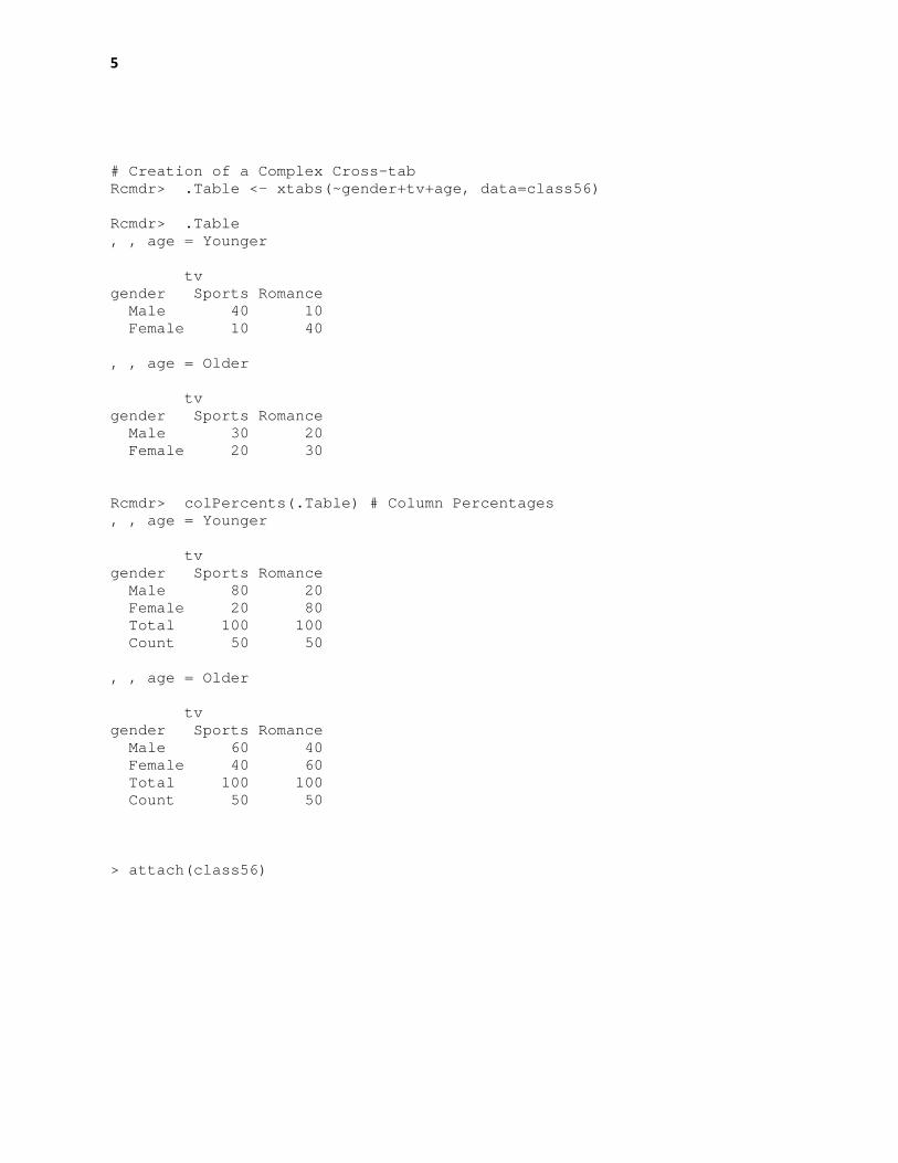
# Creation of a Complex Cross-tab Rcmdr> .Table <- xtabs(~gender+tv+age, data=class56) Rcmdr> .Table , , age = Younger tv gender Sports Romance Male 40 10 Female 10 40 , , age = Older tv gender Sports Romance Male 30 20 Female 20 30 Rcmdr> colPercents(.Table) # Column Percentages , , age = Younger tv gender Sports Romance Male 80 20 Female 20 80 Total 100 100 Count 50 50 , , age = Older tv gender Sports Romance Male 60 40 Female 40 60 Total 100 100 Count 50 50 > attach(class56)

6 

 

# Creation of A Simple Cross-tab

> table(gender,tv) tv gender Sports Romance Male 70 30 Female 30 70 > gt<-table(gender,tv) > gt tv gender Sports Romance Male 70 30 Female 30 70

7 

 

# Run logistic regression as a generalized linear model # Main effects model Rcmdr> GLM.2 <- glm(tv ~ age +gender, family=binomial(logit), data=class56) Rcmdr> summary(GLM.2) Call: glm(formula = tv ~ age + gender, family = binomial(logit), data = class56) Deviance Residuals: Min 1Q Median 3Q Max -1.5518 -0.8446 0.0000 0.8446 1.5518 Coefficients: Estimate Std. Error z value Pr(>|z|) (Intercept) -8.473e-01 2.673e-01 -3.170 0.00152 ** age[T.Older] -9.752e-17 3.086e-01 -3.16e-16 1.00000 gender[T.Female] 1.695e+00 3.086e-01 5.491 3.99e-08 *** --- Signif. codes: 0 '***' 0.001 '**' 0.01 '*' 0.05 '.' 0.1 ' ' 1 (Dispersion parameter for binomial family taken to be 1) Null deviance: 277.26 on 199 degrees of freedom Residual deviance: 244.35 on 197 degrees of freedom AIC: 250.35 # Generalized Linear Model with Interactions Rcmdr> GLM.2 <- glm(tv ~ age +gender + age*gender, family=binomial(logit), data=class56) Rcmdr> summary(GLM.2) Call: glm(formula = tv ~ age + gender + age * gender, family = binomial(logit), data = class56) Deviance Residuals: Min 1Q Median 3Q Max -1.794 -1.011 0.000 1.011 1.794 Coefficients: Estimate Std. Error z value Pr(>|z|) (Intercept) -1.3863 0.3536 -3.921 8.82e-05 *** age[T.Older] 0.9808 0.4564 2.149 0.03164 * gender[T.Female] 2.7726 0.5000 5.545 2.94e-08 *** age[T.Older]:gender[T.Female] -1.9617 0.6455 -3.039 0.00237 ** --- Signif. codes: 0 '***' 0.001 '**' 0.01 '*' 0.05 '.' 0.1 ' ' 1 (Dispersion parameter for binomial family taken to be 1) Null deviance: 277.26 on 199 degrees of freedom Residual deviance: 234.68 on 196 degrees of freedom AIC: 242.68

8 

 

# Multinomial Logistic Rcmdr> MLM.1 <- multinom(tv ~ age* gender, data=class56, trace=FALSE) Rcmdr> summary(MLM.1, cor=FALSE, Wald=TRUE) Call: multinom(formula = tv ~ age * gender, data = class56, trace = FALSE) Coefficients: Values Std. Err. Value/SE (Intercept) -1.386285 0.3535524 -3.921017 age[T.Older] 0.980823 0.4564346 2.148879 gender[T.Female] 2.772569 0.4999985 5.545154 age[T.Older]:gender[T.Female] -1.961645 0.6454960 -3.038974 Residual Deviance: 234.6828 AIC: 242.6828

9 

 

# Configural Frequency Analysis (VonEye and Others) > cfa(class56[,-1]) *** Analysis of configuration frequencies (CFA) *** label n expected Q chisq p.chisq sig.chisq z p.z sig.z 1 Younger Female Romance 40 25 0.08571429 9 0.002699796 TRUE 3.1002304 0.0009668508 TRUE 2 Younger Male Romance 10 25 0.08571429 9 0.002699796 TRUE -3.3140394 0.9995402073 TRUE 3 Younger Female Sports 10 25 0.08571429 9 0.002699796 TRUE -3.3140394 0.9995402073 TRUE 4 Younger Male Sports 40 25 0.08571429 9 0.002699796 TRUE 3.1002304 0.0009668508 TRUE 5 Older Female Romance 30 25 0.02857143 1 0.317310508 FALSE 0.9621405 0.1679895235 FALSE 6 Older Male Romance 20 25 0.02857143 1 0.317310508 FALSE -1.1759495 0.8801924645 FALSE 7 Older Female Sports 20 25 0.02857143 1 0.317310508 FALSE -1.1759495 0.8801924645 FALSE 8 Older Male Sports 30 25 0.02857143 1 0.317310508 FALSE 0.9621405 0.1679895235 FALSE Summary statistics: Total Chi squared = 40 Total degrees of freedom = 4 p = 2.539629e-10 Sum of counts = 200

10 

 

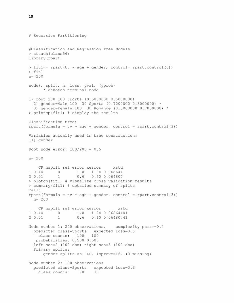
# Recursive Partitioning

#Classification and Regression Tree Models > attach(class56) library(rpart) > fit1<- rpart(tv ~ age + gender, control= rpart.control(3)) > fit1 n= 200 node), split, n, loss, yval, (yprob) * denotes terminal node 1) root 200 100 Sports (0.5000000 0.5000000) 2) gender=Male 100 30 Sports (0.7000000 0.3000000) * 3) gender=Female 100 30 Romance (0.3000000 0.7000000) * > printcp(fit1) # display the results Classification tree: rpart(formula = tv ~ age + gender, control = rpart.control(3)) Variables actually used in tree construction: [1] gender Root node error: 100/200 = 0.5 n= 200 CP nsplit rel error xerror xstd 1 0.40 0 1.0 1.24 0.068644 2 0.01 1 0.6 0.60 0.064807 > plotcp(fit1) # visualize cross-validation results > summary(fit1) # detailed summary of splits Call: rpart(formula = tv ~ age + gender, control = rpart.control(3)) n= 200 CP nsplit rel error xerror xstd 1 0.40 0 1.0 1.24 0.06864401 2 0.01 1 0.6 0.60 0.06480741 Node number 1: 200 observations, complexity param=0.4 predicted class=Sports expected loss=0.5 class counts: 100 100 probabilities: 0.500 0.500 left son=2 (100 obs) right son=3 (100 obs) Primary splits: gender splits as LR, improve=16, (0 missing) Node number 2: 100 observations predicted class=Sports expected loss=0.3 class counts: 70 30

11 

 

probabilities: 0.700 0.300 Node number 3: 100 observations predicted class=Romance expected loss=0.3 class counts: 30 70 probabilities: 0.300 0.700 # Partitioning with the party Package library(party) > fit3 <- ctree(tv ~ age + gender) > plot(fit3, main="Conditional Inference Tree for TV") Conditional inference tree with 2 terminal nodes Response: tv Inputs: age, gender Number of observations: 200 1) gender == {Male}; criterion = 1, statistic = 31.84 2)* weights = 100 1) gender == {Female} 3)* weights = 100 > # Partitioning via Random Forests Package > library(randomForest) > fit4 <- randomForest(tv ~ age + gender) > print(fit4) # view results Call: randomForest(formula = tv ~ age + gender) Type of random forest: classification Number of trees: 500 No. of variables tried at each split: 1 OOB estimate of error rate: 30% Confusion matrix: Sports Romance class.error Sports 70 30 0.3 Romance 30 70 0.3 > importance(fit4) # importance of each predictor MeanDecreaseGini age 1.418742 gender 12.862993 > plot(fit4)

12 

 

# Correspondence Analyis of a Simple Table

# Descriptions of categories Rcmdr> results=catdes(class56[,c("tv", "id", "age", "gender")] ,num.var=1,proba=0.05) RcmdrMsg: [8] ERROR: unexpected symbol in "Description by" Rcmdr> results$test.chi p.value df gender 1.541726e-08 1 RcmdrMsg: [9] ERROR: unexpected symbol in "Descrition by" Rcmdr> results$quanti $Sports v.test Mean in category Overall mean sd in category Overall sd p.value id -4.886778 80.5 100.5 56.86167 57.7343 1.024997e-06 $Romance v.test Mean in category Overall mean sd in category Overall sd p.value id 4.886778 120.5 100.5 51.3152 57.7343 1.024997e-06 RcmdrMsg: [10] ERROR: unexpected symbol in "Description by" Rcmdr> results$category $Sports Cla/Mod Mod/Cla Global p.value v.test gender=Male 70 70 50 2.310326e-08 5.586995 gender=Female 30 30 50 2.310326e-08 -5.586995 $Romance Cla/Mod Mod/Cla Global p.value v.test gender=Female 70 70 50 2.310326e-08 5.586995 gender=Male 30 30 50 2.310326e-08 -5.586995 coran1 <- anacor(class56[,-1], scaling = c("standard", "centroid")) > tabulate(age,gender) [1] 100 > ?tabulate > table(gender,tv) tv gender Sports Romance Male 70 30 Female 30 70 > gtab<-table(gender,tv)

13 

 

> anacor(gtab,ndim=1) CA fit: Sum of eigenvalues: 0.16 Benzecri RMSE rows: 0 Benzecri RMSE columns: 0 Total chi-square value: 32 Chi-Square decomposition: Chisq Proportion Cumulative Proportion Component 1 32 1 1 > ca(gtab,nd=2) Principal inertias (eigenvalues): 1 Value 0.16 Percentage 100% Rows: Male Female Mass 0.50 0.50 ChiDist 0.40 0.40 Inertia 0.08 0.08 Dim. 1 -1.00 1.00 Columns: Sports Romance Mass 0.50 0.50 ChiDist 0.40 0.40 Inertia 0.08 0.08 Dim. 1 -1.00 1.00 > coran3<-ca(gtab,nd=2) > coran3 Principal inertias (eigenvalues): 1 Value 0.16 Percentage 100% Rows: Male Female Mass 0.50 0.50 ChiDist 0.40 0.40 Inertia 0.08 0.08 Dim. 1 -1.00 1.00

14 

 

Columns: Sports Romance Mass 0.50 0.50 ChiDist 0.40 0.40 Inertia 0.08 0.08 Dim. 1 -1.00 1.00 > summary(coran3) Principal inertias (eigenvalues): dim value % cum% scree plot 1 0.160000 21.0 100.0 ************************* -------- ----- Total: 0.160000 100.0 Rows: name mass qlt inr k=1 cor ctr 1 | Male | 500 1000 500 | -400 1000 500 | 2 | Feml | 500 1000 500 | 400 1000 500 | Columns: name mass qlt inr k=1 cor ctr 1 | Sprt | 500 1000 500 | -400 1000 500 | 2 | Rmnc | 500 1000 500 | 400 1000 500 |

15 

 

# Multiple Correspondence Analysis Using Rcmdr Rcmdr> class56.MCA<-class56[, c("age", "gender", "tv")] RcmdrMsg: [4] NOTE: The dataset class56.MCA has 200 rows and 3 columns. Rcmdr> res<-MCA(class56.MCA, ncp=5, graph = FALSE) Rcmdr> plot.MCA(res, axes=c(1, 2), habillage="none", col.ind="black", Rcmdr+ col.ind.sup="blue", col.quali.sup="magenta", label=c("ind.sup", "quali.sup", Rcmdr+ "var", "quanti.sup"), invisible=c("quanti.sup","ind"), title="MCA")) Rcmdr> res$eig eigenvalue percentage of variance cumulative percentage of variance dim 1 0.4666667 46.66667 46.66667 dim 2 0.3333333 33.33333 80.00000 dim 3 0.2000000 20.00000 100.00000 Rcmdr> res$var $coord Dim 1 Dim 2 Dim 3 Dim 4 Dim 5 Younger 1.703959e-15 -1.000000e+00 -6.884856e-19 2.325331e-16 1.064425e-17 Older 1.678712e-15 1.000000e+00 -5.882747e-19 2.325331e-16 1.064425e-17 Male -8.366600e-01 -7.543967e-18 5.477226e-01 -1.251793e-17 8.448765e-18 Female 8.366600e-01 7.543967e-18 -5.477226e-01 -1.251793e-17 8.448765e-18 Sports -8.366600e-01 -7.543967e-18 -5.477226e-01 -1.870558e-17 1.266670e-16 Romance 8.366600e-01 7.543967e-18 5.477226e-01 -1.870558e-17 1.266670e-16 $contrib Dim 1 Dim 2 Dim 3 Dim 4 Dim 5 Younger 1.036956e-28 5.000000e+01 3.950103e-35 49.5358979 0.3490623 Older 1.006456e-28 5.000000e+01 2.883893e-35 49.5358979 0.3490623 Male 2.500000e+01 2.845572e-33 2.500000e+01 0.1435542 0.2199173 Female 2.500000e+01 2.845572e-33 2.500000e+01 0.1435542 0.2199173 Sports 2.500000e+01 2.845572e-33 2.500000e+01 0.3205479 49.4310204 Romance 2.500000e+01 2.845572e-33 2.500000e+01 0.3205479 49.4310204 $cos2 Dim 1 Dim 2 Dim 3 Dim 4 Dim 5 Younger 2.903478e-30 1.000000e+00 4.740124e-37 5.407162e-32 1.133000e-34 Older 2.818075e-30 1.000000e+00 3.460671e-37 5.407162e-32 1.133000e-34 Male 7.000000e-01 5.691144e-35 3.000000e-01 1.566986e-34 7.138164e-35 Female 7.000000e-01 5.691144e-35 3.000000e-01 1.566986e-34 7.138164e-35 Sports 7.000000e-01 5.691144e-35 3.000000e-01 3.498986e-34 1.604452e-32 Romance 7.000000e-01 5.691144e-35 3.000000e-01 3.498986e-34 1.604452e-32

16 

 

$v.test

Dim 1 Dim 2 Dim 3 Dim 4 Dim 5 Younger 2.403730e-14 -1.410674e+01 -9.712284e-18 3.280282e-15 1.501556e-16 Older 2.368115e-14 1.410674e+01 -8.298636e-18 3.280282e-15 1.501556e-16 Male -1.180254e+01 -1.064208e-16 7.726578e+00 -1.765872e-16 1.191845e-16 Female 1.180254e+01 1.064208e-16 -7.726578e+00 -1.765872e-16 1.191845e-16 Sports -1.180254e+01 -1.064208e-16 -7.726578e+00 -2.638746e-16 1.786857e-15 Romance 1.180254e+01 1.064208e-16 7.726578e+00 -2.638746e-16 1.786857e-15 $eta2 Dim 1 Dim 2 Dim 3 Dim 4 Dim 5 age 6.215505e-34 1.000000e+00 2.559879e-34 1.785866e-31 2.932898e-34 gender 7.000000e-01 5.596074e-34 3.000000e-01 5.909984e-32 7.106369e-34 tv 7.000000e-01 5.596074e-34 3.000000e-01 5.909984e-32 6.005247e-33 # MCA Dimension description Rcmdr> dimdesc(res, axes=c(1, 2)) $`Dim 1` $`Dim 1`$quali R2 p.value gender 0.7 1.160349e-53 tv 0.7 1.160349e-53 $`Dim 1`$category Estimate p.value Romance 0.5715476 1.160349e-53 Female 0.5715476 1.160349e-53 Sports -0.5715476 1.160349e-53 Male -0.5715476 1.160349e-53 $`Dim 2` $`Dim 2`$quali R2 p.value age 1 0 $`Dim 2`$category Estimate p.value Older 0.5773503 0 Younger -0.5773503 0

17 

 

# Mutliple Correspondewnce Analysis MCA Using homals > library(homals) Call: homals(data = class56, ndim = 2) Loss: 0.001 Eigenvalues: D1 D2 0.0778 0.0556 Variable Loadings: D1 D2 age -0.004928463 -0.577329214 gender -0.483028361 0.004042007 tv -0.483028222 0.004204889 > plot(homclas) > homclas<-homals(class56,ndim=2,sets=list(1:2,3)) > homclas Call: homals(data = class56, ndim = 2, sets = list(1:2, 3)) Loss: 0.0006666667 Eigenvalues: D1 D2 0.175 0.125 Variable Loadings: D1 D2 age -0.004311584 -0.707093628 gender -0.591597017 0.003547484 tv -0.591596944 0.003667175 > summary(homclas) Number of dimensions: 2 Number of iterations: 17 Variable: age Loadings: D1 D2 1 -0.0043 -0.7071 Category centroids: D1 D2 Older 3e-04 0.05 Younger -3e-04 -0.05 Category quantifications (scores): D1 D2 Older 3e-04 0.05 Younger -3e-04 -0.05

18 

 

Lower rank quantifications (rank = 1): 1 Older -0.0707 Younger 0.0707 --------- Variable: gender Loadings: D1 D2 1 -0.5916 0.0035 Category centroids: D1 D2 Female 0.0418 -3e-04 Male -0.0418 3e-04 Category quantifications (scores): D1 D2 Female 0.0418 -3e-04 Male -0.0418 3e-04 Lower rank quantifications (rank = 1): 1 Female -0.0707 Male 0.0707 --------- Variable: tv Loadings: D1 D2 1 -0.5916 0.0037 Category centroids: D1 D2 Romance 0.0418 -3e-04 Sports -0.0418 3e-04 Category quantifications (scores): D1 D2 Romance 0.0418 -3e-04 Sports -0.0418 3e-04 Lower rank quantifications (rank = 1): 1 Romance -0.0707 Sports 0.0707

19 

 

# Multiple Joint Correspondence Analysis

> mjca(class56[,-1]) > mjcoran<-mjca(class56[,-1],lambda="Burt") > summary(mjcoran) Principal inertias (eigenvalues): dim value % cum% scree plot 1 0.217778 59.0 59.0 ************************* 2 0.111111 30.1 89.2 ********** 3 0.040000 10.8 100.0 -------- ----- Total: 0.368889 100.0 Columns: name mass qlt inr k=1 cor ctr k=2 cor ctr 1 | ageYounger | 167 1000 151 | 0 0 0 | 577 1000 167 | 2 | ageOlder | 167 1000 151 | 0 0 0 | -577 1000 167 | 3 | genderMale | 167 845 175 | 572 845 117 | 0 0 0 | 4 | genderFemale | 167 845 175 | -572 845 117 | 0 0 0 | 5 | tvSports | 167 845 175 | 572 845 117 | 0 0 0 | 6 | tvRomance | 167 845 175 | -572 845 117 | 0 0 0 | > plot(mjcoran) > plot(mjcoran,cex=.5) > plot(mjcoran,cex=2.5) > plot(mjcoran,cex=0.3)

20 

 

#Latent Class Analysis # Latent Class using polCA > library(poLCA) > M0<-poLCA(formu,class56[,-1],nclass=2) Conditional item response (column) probabilities, by outcome variable, for each class (row) $gender Pr(1) Pr(2) class 1: 1.0 0.0 class 2: 0.3 0.7 $tv Pr(1) Pr(2) class 1: 1.0 0.0 class 2: 0.3 0.7 $age Pr(1) Pr(2) class 1: 0.5962 0.4038 class 2: 0.4615 0.5385 Estimated class population shares 0.2857 0.7143 Predicted class memberships (by modal posterior prob.) 0.35 0.65 ========================================================= Fit for 2 latent classes: ========================================================= number of observations: 200 number of estimated parameters: 7 residual degrees of freedom: 0 maximum log-likelihood: -398.33 AIC(2): 810.66 BIC(2): 833.7482 G^2(2): 7.459441 (Likelihood ratio/deviance statistic) X^2(2): 7.369615 (Chi-square goodness of fit) > > formu<-cbind(gender,tv,age)~1 > M3<-poLCA(formu,class56[,-1],nclass=4) Conditional item response (column) probabilities, by outcome variable, for each class (row)

21 

 

$gender Pr(1) Pr(2) class 1: 0.9367 0.0633 class 2: 0.6849 0.3151 class 3: 0.2712 0.7288 class 4: 0.0893 0.9107 $tv Pr(1) Pr(2) class 1: 0.9600 0.0400 class 2: 0.5566 0.4434 class 3: 0.4468 0.5532 class 4: 0.0558 0.9442 $age Pr(1) Pr(2) class 1: 0.7939 0.2061 class 2: 0.2097 0.7903 class 3: 0.2487 0.7513 class 4: 0.7687 0.2313 Estimated class population shares 0.2376 0.283 0.224 0.2553 Predicted class memberships (by modal posterior prob.) 0.2 0.3 0.3 0.2 ========================================================= Fit for 4 latent classes: ========================================================= number of observations: 200 number of estimated parameters: 15 residual degrees of freedom: -8 maximum log-likelihood: -394.6003 AIC(4): 819.2006 BIC(4): 868.6753 G^2(4): 3.486525e-10 (Likelihood ratio/deviance statistic) X^2(4): 3.485955e-10 (Chi-square goodness of fit) ALERT: negative degrees of freedom; respecify model > formu<-cbind(gender,tv,age)~1 > M4<-poLCA(formu,class56[,-1],nclass=3) Conditional item response (column) probabilities, by outcome variable, for each class (row) $gender Pr(1) Pr(2) class 1: 0.0735 0.9265 class 2: 0.5003 0.4997 class 3: 0.8490 0.1510

22 

 

$tv Pr(1) Pr(2) class 1: 0.0357 0.9643 class 2: 0.5003 0.4997 class 3: 0.8799 0.1201 $age Pr(1) Pr(2) class 1: 0.7498 0.2502 class 2: 0.0971 0.9029 class 3: 0.7503 0.2497 Estimated class population shares 0.2778 0.383 0.3392 Predicted class memberships (by modal posterior prob.) 0.2 0.5 0.3 ========================================================= Fit for 3 latent classes: ========================================================= number of observations: 200 number of estimated parameters: 11 residual degrees of freedom: -4 maximum log-likelihood: -394.6003 AIC(3): 811.2006 BIC(3): 847.482 G^2(3): 9.215952e-10 (Likelihood ratio/deviance statistic) X^2(3): 9.222167e-10 (Chi-square goodness of fit) ALERT: negative degrees of freedom; respecify model > plot(M0) > M0$predcell gender tv age observed expected 1 1 1 1 40 40.000 2 1 1 2 30 30.000 3 1 2 1 10 13.846 4 1 2 2 20 16.154 5 2 1 1 10 13.846 6 2 1 2 20 16.154 7 2 2 1 40 32.308 8 2 2 2 30 37.692 > M0$p NULL > M0$y gender tv age 1 1 1 1 2 1 1 1 3 1 1 1 4 1 1 1 5 1 1 1

23 

 

# Item Response Theory Fit # Notice that these are numeric values Rcmdr> summary(class7) id age gender tv Min. : 1.00 Min. :1.0 Min. :1.0 Min. :1.0 1st Qu.: 50.75 1st Qu.:1.0 1st Qu.:1.0 1st Qu.:1.0 Median :100.50 Median :1.5 Median :1.5 Median :1.5 Mean :100.50 Mean :1.5 Mean :1.5 Mean :1.5 3rd Qu.:150.25 3rd Qu.:2.0 3rd Qu.:2.0 3rd Qu.:2.0 Max. :200.00 Max. :2.0 Max. :2.0 Max. :2.0 > class7a<-as.matrix(class7) > ltm(class7a ~ L1) Error in eval(expr, envir, enclos) : object 'L1' not found > ltm(class7a ~ z1) Error in ltm(class7a ~ z1) : 'data' contain more that 2 distinct values for item(s): 1 # Dropt the id column > class7b<-class7a[,-1] # Postulate One latent dimension > ltm(class7b ~ z1) Call: ltm(formula = class7b ~ z1) Coefficients: Dffclt Dscrmn age 0 0.000 gender 0 -2.032 tv 0 -2.032 Log.Lik: -399.432 > irtdem<-ltm(class7b ~ z1) > irtdem Call: ltm(formula = class7b ~ z1) Coefficients: Dffclt Dscrmn age 0 0.000 gender 0 -2.032 tv 0 -2.032 Log.Lik: -399.432

24 

 

> summary(irtdem) Call: ltm(formula = class7b ~ z1) Model Summary: log.Lik AIC BIC -399.4317 810.8635 830.6534 Coefficients: value std.err z.vals Dffclt.age 0.0001 1.095250e+10 0.0000 Dffclt.gender 0.0000 1.160000e-01 0.0000 Dffclt.tv 0.0000 1.160000e-01 0.0000 Dscrmn.age 0.0000 1.942000e-01 0.0000 Dscrmn.gender -2.0320 5.834211e+02 -0.0035 Dscrmn.tv -2.0320 5.834211e+02 -0.0035 Integration: method: Gauss-Hermite quadrature points: 21 Optimization: Convergence: 0 max(|grad|): <1e-06 quasi-Newton: BFGS > coef(irtdem) Dffclt Dscrmn age 5.686497e-05 1.291224e-11 gender 2.886472e-11 -2.031994e+00 tv 2.886472e-11 -2.031994e+00