R Code for Data

Manipulation

Avjinder Singh Kaler

Table Content

1. Creating, Recoding and Renaming variables

2. Operators

3. Built-in Functions

4. Sorting, Merging and Aggregating Data

5. Reshaping Data

6. Sub-setting Data

Introduction

Data manipulation in R includes creating new

(including recoding and renaming existing variables

variables), sorting and merging datasets, aggregating

data, reshaping data, and subsetting datasets

(including selecting observations that meet criteria,

randomly sampling observeration, and dropping or

keeping variables).

Suppose you have a dataset (mydata) with three variables

x1, x2 and x3.

Old

Variables

New

Variables

Sorting and Merge

Aggregating

Recode and Reshaping

Transform

Subsetting

Data

Frame

1. Creating, Recoding and Renaming variables

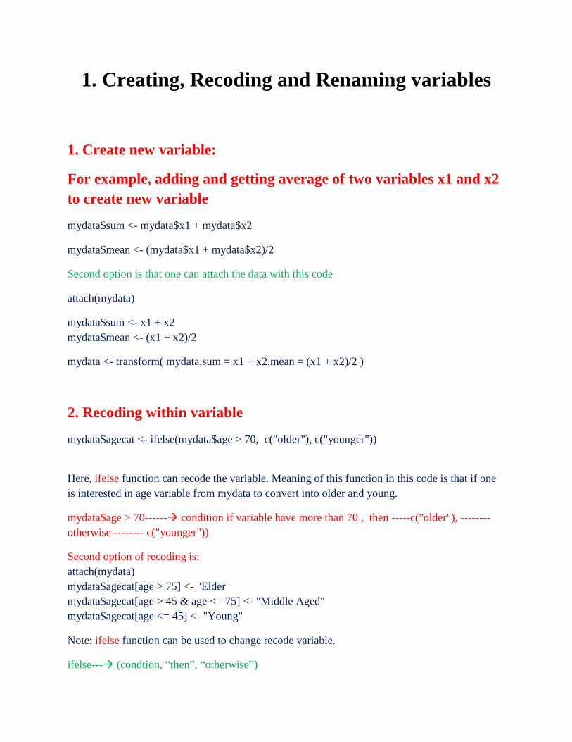
1. Create new variable:

For example, adding and getting average of two variables x1 and x2

to create new variable

mydata$sum <- mydata$x1 + mydata$x2

mydata$mean <- (mydata$x1 + mydata$x2)/2

Second option is that one can attach the data with this code

attach(mydata)

mydata$sum <- x1 + x2

mydata$mean <- (x1 + x2)/2

mydata <- transform( mydata,sum = x1 + x2,mean = (x1 + x2)/2 )

2. Recoding within variable

mydata$agecat <- ifelse(mydata$age > 70, c("older"), c("younger"))

Here, ifelse function can recode the variable. Meaning of this function in this code is that if one

is interested in age variable from mydata to convert into older and young.

mydata$age > 70------ condition if variable have more than 70 , then -----c("older"), --------

otherwise -------- c("younger"))

Second option of recoding is:

attach(mydata)

mydata$agecat[age > 75] <- "Elder"

mydata$agecat[age > 45 & age <= 75] <- "Middle Aged"

mydata$agecat[age <= 45] <- "Young"

Note: ifelse function can be used to change recode variable.

ifelse--- (condtion, “then”, “otherwise”)

3. Renaming the variables

Two ways to rename variables, interactively and programmatically

# rename interactively

fix(mydata) # results are saved on close

# rename programmatically

library(reshape)

mydata <- rename(mydata, c(oldname="newname"))

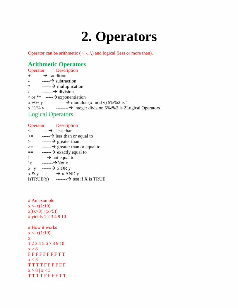
2. Operators Operator can be arithmetic (+, -, /,) and logical (less or more than).

Arithmetic Operators Operator Description

+ ----- addition

- ----- subtraction

* ------ multiplication

/ ------- division

^ or ** -----exponentiation

x %% y ------ modulus (x mod y) 5%%2 is 1

x %/% y -------- integer division 5%/%2 is 2Logical Operators

Logical Operators

Operator Description

< ---- less than

<= ----- less than or equal to

> ------ greater than

>= ------ greater than or equal to

== ------ exactly equal to

!= --- not equal to

!x -------Not x

x | y ------ x OR y

x & y --------- x AND y

isTRUE(x) ------- test if X is TRUE

# An example

x <- c(1:10)

x[(x>8) | (x<5)]

# yields 1 2 3 4 9 10

# How it works

x <- c(1:10)

x

1 2 3 4 5 6 7 8 9 10

x > 8

F F F F F F F F T T

x < 5

T T T T F F F F F F

x > 8 | x < 5

T T T T F F F F T T

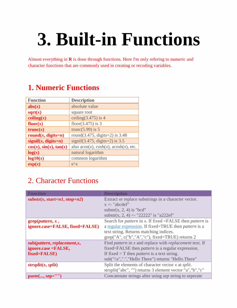
3. Built-in Functions Almost everything in R is done through functions. Here I'm only refering to numeric and

character functions that are commonly used in creating or recoding variables.

1. Numeric Functions

Function Description

abs(x) absolute value

sqrt(x) square root

ceiling(x) ceiling(3.475) is 4

floor(x) floor(3.475) is 3

trunc(x) trunc(5.99) is 5

round(x, digits=n) round(3.475, digits=2) is 3.48

signif(x, digits=n) signif(3.475, digits=2) is 3.5

cos(x), sin(x), tan(x) also acos(x), cosh(x), acosh(x), etc.

log(x) natural logarithm

log10(x) common logarithm

exp(x) e^x

2. Character Functions

Function Description

substr(x, start=n1, stop=n2) Extract or replace substrings in a character vector.

x <- "abcdef"

substr(x, 2, 4) is "bcd"

substr(x, 2, 4) <- "22222" is "a222ef"

grep(pattern, x ,

ignore.case=FALSE, fixed=FALSE)

Search for pattern in x. If fixed =FALSE then pattern is

a regular expression. If fixed=TRUE then pattern is a

text string. Returns matching indices.

grep("A", c("b","A","c"), fixed=TRUE) returns 2

sub(pattern, replacement,x,

ignore.case =FALSE,

fixed=FALSE)

Find pattern in x and replace with replacement text. If

fixed=FALSE then pattern is a regular expression.

If fixed = T then pattern is a text string.

sub("\\s",".","Hello There") returns "Hello.There"

strsplit(x, split) Split the elements of character vector x at split.

strsplit("abc", "") returns 3 element vector "a","b","c"

paste(..., sep="") Concatenate strings after using sep string to seperate

them.

paste("x",1:3,sep="") returns c("x1","x2" "x3")

paste("x",1:3,sep="M") returns c("xM1","xM2" "xM3")

paste("Today is", date())

toupper(x) Uppercase

tolower(x) Lowercase

3. Statistical Probability Functions

Function Description

dnorm(x) normal density function (by default m=0 sd=1)

# plot standard normal curve

x <- pretty(c(-3,3), 30)

y <- dnorm(x)

plot(x, y, type='l', xlab="Normal Deviate", ylab="Density", yaxs="i")

pnorm(q) cumulative normal probability for q

(area under the normal curve to the left of q)

pnorm(1.96) is 0.975

qnorm(p) normal quantile.

value at the p percentile of normal distribution

qnorm(.9) is 1.28 # 90th percentile

rnorm(n, m=0,sd=1) n random normal deviates with mean m

and standard deviation sd.

#50 random normal variates with mean=50, sd=10

x <- rnorm(50, m=50, sd=10)

dbinom(x, size, prob)

pbinom(q, size, prob)

qbinom(p, size, prob)

rbinom(n, size, prob)

binomial distribution where size is the sample size

and prob is the probability of a heads (pi)

# prob of 0 to 5 heads of fair coin out of 10 flips

dbinom(0:5, 10, .5)

# prob of 5 or less heads of fair coin out of 10 flips

pbinom(5, 10, .5)

dpois(x, lamda)

ppois(q, lamda)

qpois(p, lamda)

rpois(n, lamda)

poisson distribution with m=std=lamda

#probability of 0,1, or 2 events with lamda=4

dpois(0:2, 4)

# probability of at least 3 events with lamda=4

1- ppois(2,4)

dunif(x, min=0, max=1)

punif(q, min=0, max=1)

qunif(p, min=0, max=1)

runif(n, min=0, max=1)

uniform distribution, follows the same pattern

as the normal distribution above.

#10 uniform random variates

x <- runif(10)

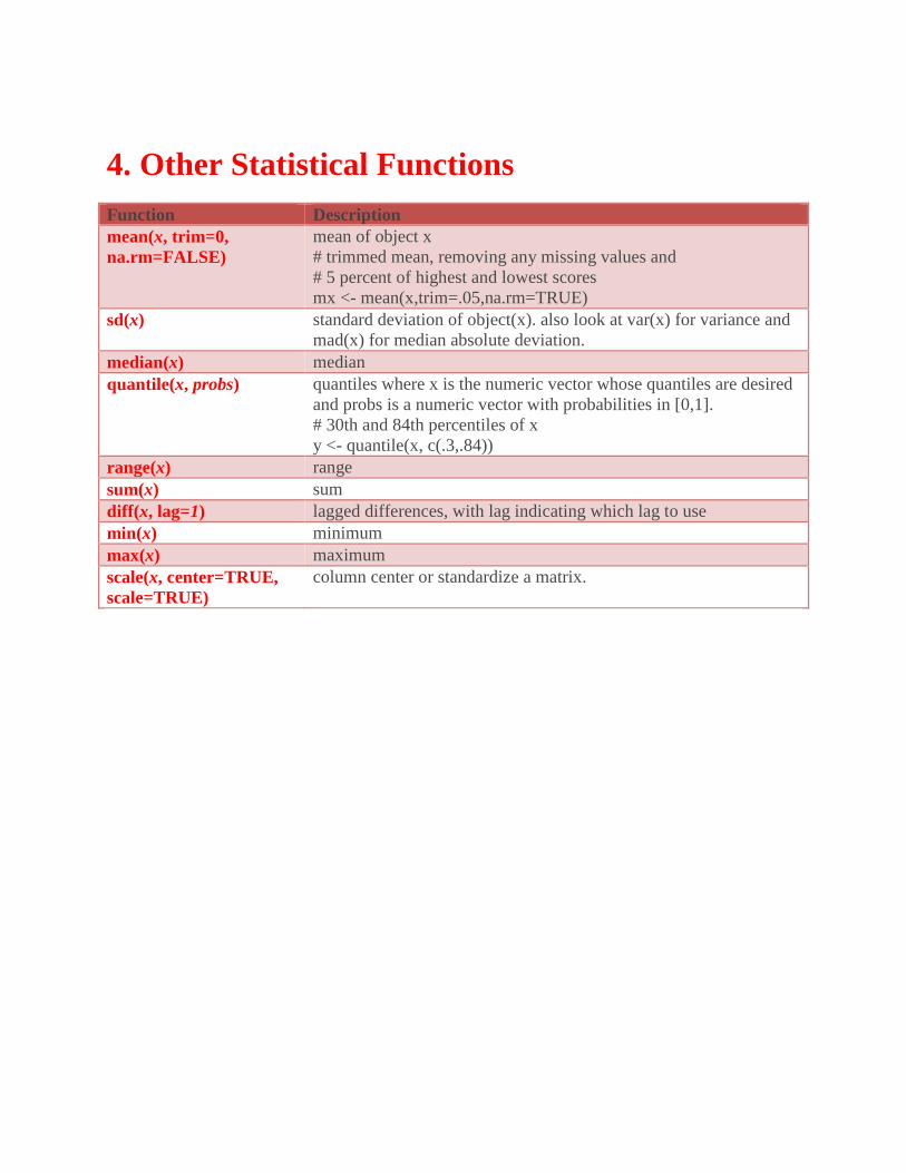
4. Other Statistical Functions

Function Description

mean(x, trim=0,

na.rm=FALSE)

mean of object x

# trimmed mean, removing any missing values and

# 5 percent of highest and lowest scores

mx <- mean(x,trim=.05,na.rm=TRUE)

sd(x) standard deviation of object(x). also look at var(x) for variance and

mad(x) for median absolute deviation.

median(x) median

quantile(x, probs) quantiles where x is the numeric vector whose quantiles are desired

and probs is a numeric vector with probabilities in [0,1].

# 30th and 84th percentiles of x

y <- quantile(x, c(.3,.84))

range(x) range

sum(x) sum

diff(x, lag=1) lagged differences, with lag indicating which lag to use

min(x) minimum

max(x) maximum

scale(x, center=TRUE,

scale=TRUE)

column center or standardize a matrix.

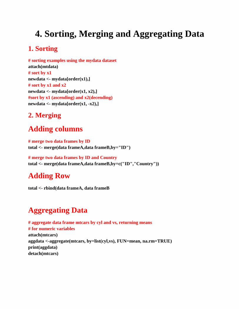
4. Sorting, Merging and Aggregating Data

1. Sorting

# sorting examples using the mydata dataset

attach(mtdata)

# sort by x1

newdata <- mydata[order(x1),]

# sort by x1 and x2

newdata <- mydata[order(x1, x2),]

#sort by x1 (ascending) and x2(decending)

newdata <- mydata[order(x1, -x2),]

2. Merging

Adding columns

# merge two data frames by ID

total <- merge(data frameA,data frameB,by="ID")

# merge two data frames by ID and Country

total <- merge(data frameA,data frameB,by=c("ID","Country"))

Adding Row

total <- rbind(data frameA, data frameB

Aggregating Data

# aggregate data frame mtcars by cyl and vs, returning means

# for numeric variables

attach(mtcars)

aggdata <-aggregate(mtcars, by=list(cyl,vs), FUN=mean, na.rm=TRUE)

print(aggdata)

detach(mtcars)

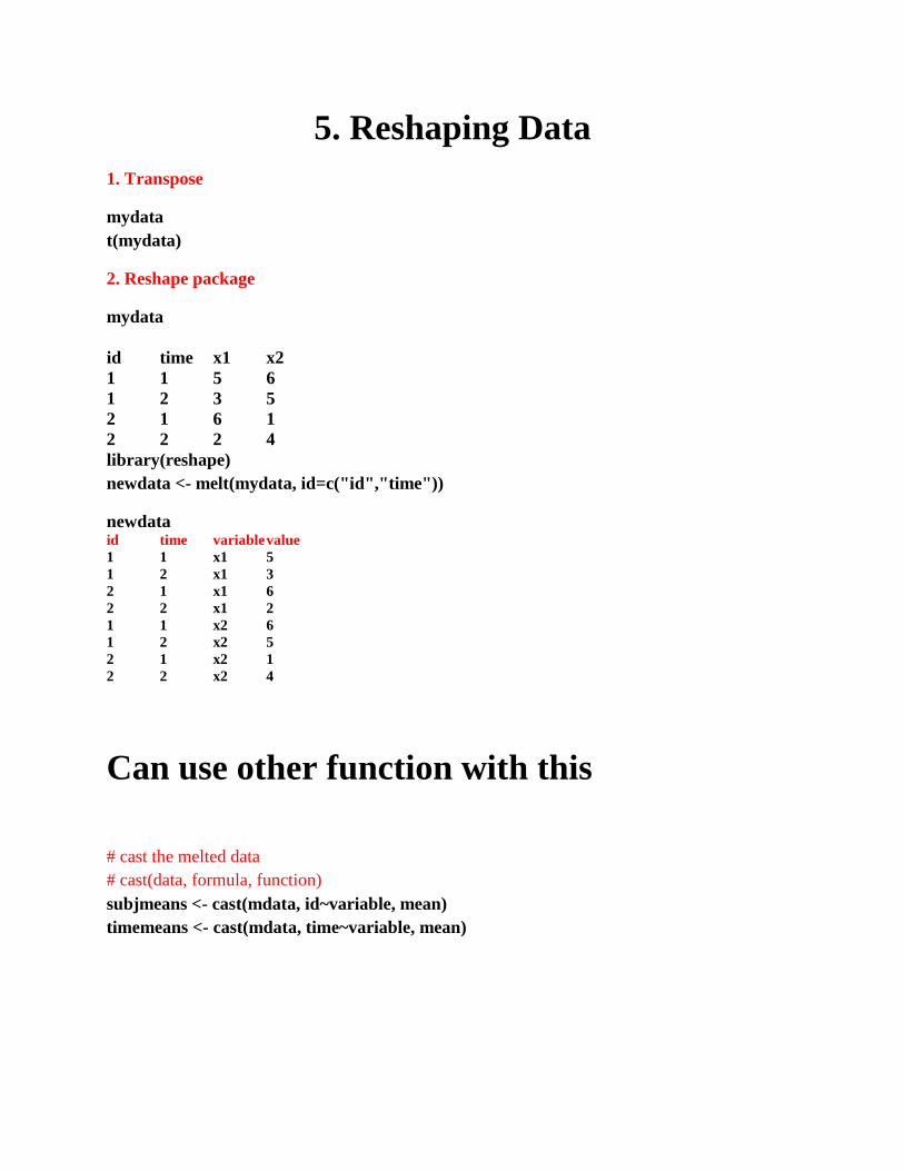
5. Reshaping Data

1. Transpose

mydata

t(mydata)

2. Reshape package

mydata

id time x1 x2

1 1 5 6

1 2 3 5

2 1 6 1

2 2 2 4

library(reshape)

newdata <- melt(mydata, id=c("id","time"))

newdata

id time variable value

1 1 x1 5

1 2 x1 3

2 1 x1 6

2 2 x1 2

1 1 x2 6

1 2 x2 5

2 1 x2 1

2 2 x2 4

Can use other function with this

# cast the melted data

# cast(data, formula, function)

subjmeans <- cast(mdata, id~variable, mean)

timemeans <- cast(mdata, time~variable, mean)

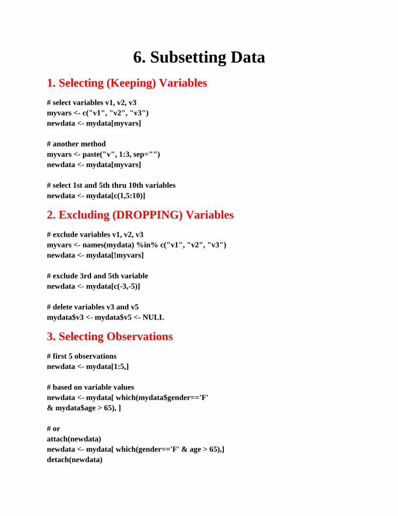
6. Subsetting Data

1. Selecting (Keeping) Variables

# select variables v1, v2, v3

myvars <- c("v1", "v2", "v3")

newdata <- mydata[myvars]

# another method

myvars <- paste("v", 1:3, sep="")

newdata <- mydata[myvars]

# select 1st and 5th thru 10th variables

newdata <- mydata[c(1,5:10)]

2. Excluding (DROPPING) Variables

# exclude variables v1, v2, v3

myvars <- names(mydata) %in% c("v1", "v2", "v3")

newdata <- mydata[!myvars]

# exclude 3rd and 5th variable

newdata <- mydata[c(-3,-5)]

# delete variables v3 and v5

mydata$v3 <- mydata$v5 <- NULL

3. Selecting Observations

# first 5 observations

newdata <- mydata[1:5,]

# based on variable values

newdata <- mydata[ which(mydata$gender=='F'

& mydata$age > 65), ]

# or

attach(newdata)

newdata <- mydata[ which(gender=='F' & age > 65),]

detach(newdata)

4. Selection using the Subset Function

# using subset function

newdata <- subset(mydata, age >= 20 | age < 10,

select=c(ID, Weight))

# using subset function (part 2)

newdata <- subset(mydata, sex=="m" & age > 25,

select=weight:income)