Quill: Efficient, Transferable, and Rich Analytics at Scale

Badrish Chandramouli†, Raul Castro Fernandez‡∗, Jonathan Goldstein†,Ahmed Eldawy]∗, Abdul Quamar◦∗

†Microsoft Research ‡MIT ]Univ. of Minnesota ◦Univ. of Marylandbadrishc@microsoft.com, raulcf@csail.mit.edu, jongold@microsoft.com, eldawy@cs.umn.edu, abdul@cs.umd.edu

ABSTRACTThis paper introduces Quill (stands for a quadrillion tuples per day),a library and distributed platform for relational and temporal analyt-ics over large datasets in the cloud. Quill exposes a new abstractionfor parallel datasets and computation, called ShardedStreamable.This abstraction provides the ability to express efficient distributedphysical query plans that are transferable, i.e., movable from offlineto real-time and vice versa. ShardedStreamable decouples incremen-tal query logic specification, a small but rich set of data movementoperations, and keying; this allows Quill to express a broad spaceof plans with complex querying functionality, while leveraging ex-isting temporal libraries such as Trill. Quill’s layered architectureprovides a careful separation of responsibilities with independentlyuseful components, while retaining high performance. We builtQuill for the cloud, with a master-less design where a language-integrated client library directly communicates and coordinates withcloud workers using off-the-shelf distributed cloud componentssuch as queues. Experiments on up to 400 cloud machines, and ondatasets up to 1TB, find Quill to incur low overheads and outper-form SparkSQL by up to orders-of-magnitude for temporal and 6×for relational queries, while supporting a rich space of transferable,programmable, and expressive distributed physical query plans.

1. INTRODUCTIONWith the growth in data volumes acquired by businesses today,

there is a need to deploy rich analytic workflows over the data, thatcan operate on both historical (bounded) and real-time (unbounded)datasets. Queries in such workflows usually take the form of:1. Ad-hoc queries, one-time queries over the data that often come

with the expectation of results at interactive latencies.2. Recurring queries, queries that are carefully authored and de-

ployed to recur periodically, such as daily or hourly reports.3. Continuous queries, queries that execute and incrementally com-

pute results over data as it is received in real-time, and may beback-tested over historical data as well.

Queries are typically issued using a declarative front-end such asSQL (or its temporal dialect), sometimes with integration into the

*Work performed during internships at Microsoft Research. AhmedEldawy is currently at the University of California, Riverside. AbdulQuamar is currently at IBM Research, Almaden.

This work is licensed under the Creative Commons Attribution-NonCommercial-NoDerivatives 4.0 International License. To view a copyof this license, visit http://creativecommons.org/licenses/by-nc-nd/4.0/. Forany use beyond those covered by this license, obtain permission by emailinginfo@vldb.org.Proceedings of the VLDB Endowment, Vol. 9, No. 14Copyright 2016 VLDB Endowment 2150-8097/16/10.

high-level language (HLL) of the application (e.g., SparkSQL [8]).Queries eventually get deployed as distributed physical plans thatexecute on a multi-node cluster. While ad-hoc queries are well-supported by such a traditional DBMS workflow, our experiencewith production large-scale uses of Trill [15], a temporal analyticslibrary used across Microsoft, indicates that customers who authorlarge-scale continuous queries (on real-time data and offline datafor back-testing) or recurring queries (on offline data) have a uniquecombination of new requirements. Consider an example scenario:

Example (Ad Platform). Consider an advertising (ad) platformthat tracks user activity such as ads shown and clicks on the ads.

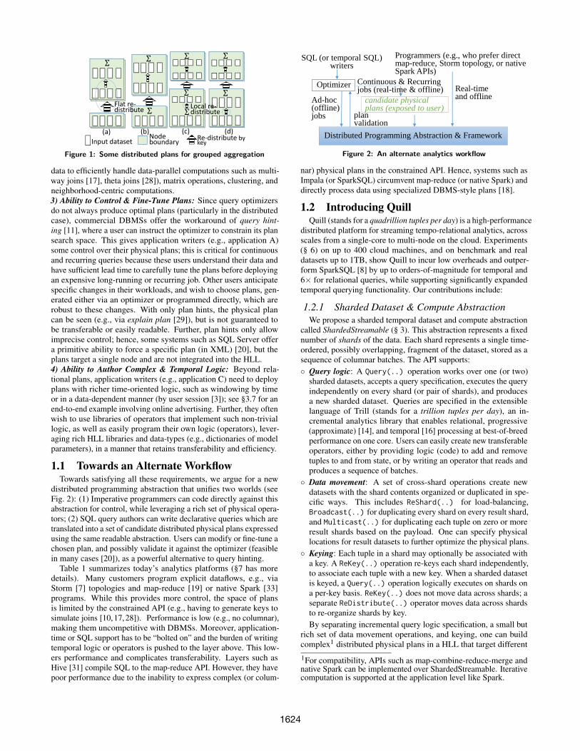
(1) Application A may wish to compute an hourly report of theper-ad count of user activity over a historical dataset, in a cluster ofmulti-core machines holding fragments of the dataset (one per core),using a combination of per-core and per-machine aggregation andshuffling data by key. Fig. 1 shows some strategies; in Fig. 1(a),we globally shuffle the dataset so that each core in the system hasa partition (by AdId) of the dataset, and then perform a per-coreaggregation. This can be appropriate if aggregation is very expen-sive. On the other hand, if we have very few groups (AdId values),Fig. 1(b) first computes an independent partial aggregate per-core,and then shuffles the aggregated results across the cluster (the otherstrategies, and more complex examples are covered in §3).

(2) Application B may want the same per-ad count query to in-stead produce an incrementally maintained dashboard of top ads inthe last 5 minutes, updated every minute. Developers may also needto back-test the query on varying amounts of offline logs at differentscales to tune the window size or other (e.g., spam) threshold.

(3) Application C may compute a per-ad recommender model [13]based on user-session-based activities, leveraging machine learninglibraries over varying windows, on either offline or real-time data.

Writers of such applications have several unique requirements:

1) Ability to Create Transferable Plans and Logic: Applicationwriters (e.g., application B) need the ability to transfer or opera-tionalize their offline logic to execute directly over real-time data(or vice versa), with carefully tuned distributed physical plans. Theywish to avoid maintaining multiple workflows and systems [25] withan ability to create plans that are transferable, i.e., the plans can bemoved from offline to real-time deployments and vice versa.2) Ability to Execute a Rich Space of Plans: Application writers(e.g., application A) expect high performance with a rich spaceof plans that exploit intra- and inter-node parallelism, as well ascolumnar [15] execution for performance. Beyond shuffle- orbroadcast-based relational plans such as the per-ad count exam-ple, one may wish to deploy diverse distributed plans that replicatedata in specific ways across machines, such as partial duplication of

1623

Σ

⋈

Node boundary

Re-distribute bykey

Σ

Σ

Σ

Σ

⋈

Σ

Σ

(a) (b) (c) (d)

Σ

Local re-distribute

Flat re-distribute

Input dataset

Figure 1: Some distributed plans for grouped aggregation

data to efficiently handle data-parallel computations such as multi-way joins [17], theta joins [28]), matrix operations, clustering, andneighborhood-centric computations.3) Ability to Control & Fine-Tune Plans: Since query optimizersdo not always produce optimal plans (particularly in the distributedcase), commercial DBMSs offer the workaround of query hint-ing [11], where a user can instruct the optimizer to constrain its plansearch space. This gives application writers (e.g., application A)some control over their physical plans; this is critical for continuousand recurring queries because these users understand their data andhave sufficient lead time to carefully tune the plans before deployingan expensive long-running or recurring job. Other users anticipatespecific changes in their workloads, and wish to choose plans, gen-erated either via an optimizer or programmed directly, which arerobust to these changes. With only plan hints, the physical plancan be seen (e.g., via explain plan [29]), but is not guaranteed tobe transferable or easily readable. Further, plan hints only allowimprecise control; hence, some systems such as SQL Server offera primitive ability to force a specific plan (in XML) [20], but theplans target a single node and are not integrated into the HLL.4) Ability to Author Complex & Temporal Logic: Beyond rela-tional plans, application writers (e.g., application C) need to deployplans with richer time-oriented logic, such as windowing by timeor in a data-dependent manner (by user session [3]); see §3.7 for anend-to-end example involving online advertising. Further, they oftenwish to use libraries of operators that implement such non-triviallogic, as well as easily program their own logic (operators), lever-aging rich HLL libraries and data-types (e.g., dictionaries of modelparameters), in a manner that retains transferability and efficiency.

1.1 Towards an Alternate WorkflowTowards satisfying all these requirements, we argue for a new

distributed programming abstraction that unifies two worlds (seeFig. 2): (1) Imperative programmers can code directly against thisabstraction for control, while leveraging a rich set of physical opera-tors; (2) SQL query authors can write declarative queries which aretranslated into a set of candidate distributed physical plans expressedusing the same readable abstraction. Users can modify or fine-tune achosen plan, and possibly validate it against the optimizer (feasiblein many cases [20]), as a powerful alternative to query hinting.

Table 1 summarizes today’s analytics platforms (§7 has moredetails). Many customers program explicit dataflows, e.g., viaStorm [7] topologies and map-reduce [19] or native Spark [33]programs. While this provides more control, the space of plansis limited by the constrained API (e.g., having to generate keys tosimulate joins [10,17,28]). Performance is low (e.g., no columnar),making them uncompetitive with DBMSs. Moreover, application-time or SQL support has to be “bolted on” and the burden of writingtemporal logic or operators is pushed to the layer above. This low-ers performance and complicates transferability. Layers such asHive [31] compile SQL to the map-reduce API. However, they havepoor performance due to the inability to express complex (or colum-

plan validation

Continuous & Recurring jobs (real-time & offline) Real-time

and offline

Distributed Programming Abstraction & Framework

Ad-hoc(offline)jobs

Optimizer

SQL (or temporal SQL)writers

Programmers (e.g., who prefer direct map-reduce, Storm topology, or native Spark APIs)

candidate physicalplans (exposed to user)

Figure 2: An alternate analytics workflow

nar) physical plans in the constrained API. Hence, systems such asImpala (or SparkSQL) circumvent map-reduce (or native Spark) anddirectly process data using specialized DBMS-style plans [18].

1.2 Introducing QuillQuill (stands for a quadrillion tuples per day) is a high-performance

distributed platform for streaming tempo-relational analytics, acrossscales from a single-core to multi-node on the cloud. Experiments(§ 6) on up to 400 cloud machines, and on benchmark and realdatasets up to 1TB, show Quill to incur low overheads and outper-form SparkSQL [8] by up to orders-of-magnitude for temporal and6× for relational queries, while supporting significantly expandedtemporal querying functionality. Our contributions include:

1.2.1 Sharded Dataset & Compute AbstractionWe propose a sharded temporal dataset and compute abstraction

called ShardedStreamable (§ 3). This abstraction represents a fixednumber of shards of the data. Each shard represents a single time-ordered, possibly overlapping, fragment of the dataset, stored as asequence of columnar batches. The API supports:◦ Query logic: A Query(..) operation works over one (or two)

sharded datasets, accepts a query specification, executes the queryindependently on every shard (or pair of shards), and producesa new sharded dataset. Queries are specified in the extensiblelanguage of Trill (stands for a trillion tuples per day), an in-cremental analytics library that enables relational, progressive(approximate) [14], and temporal [16] processing at best-of-breedperformance on one core. Users can easily create new transferableoperators, either by providing logic (code) to add and removetuples to and from state, or by writing an operator that reads andproduces a sequence of batches.◦ Data movement: A set of cross-shard operations create new

datasets with the shard contents organized or duplicated in spe-cific ways. This includes ReShard(..) for load-balancing,Broadcast(..) for duplicating every shard on every result shard,and Multicast(..) for duplicating each tuple on zero or moreresult shards based on the payload. One can specify physicallocations for result datasets to further optimize the physical plans.◦ Keying: Each tuple in a shard may optionally be associated with

a key. A ReKey(..) operation re-keys each shard independently,to associate each tuple with a new key. When a sharded datasetis keyed, a Query(..) operation logically executes on shards ona per-key basis. ReKey(..) does not move data across shards; aseparate ReDistribute(..) operator moves data across shardsto re-organize shards by key.By separating incremental query logic specification, a small but

rich set of data movement operations, and keying, one can buildcomplex1 distributed physical plans in a HLL that target different

1For compatibility, APIs such as map-combine-reduce-merge andnative Spark can be implemented over ShardedStreamable. Iterativecomputation is supported at the application level like Spark.

1624

Table 1: Sample of today’s solutions for distributed analytics

Requirement Map-reduce Hive

Trad.DB,Impala

SparkSQL

NativeSpark

Data-flow,Flink

Storm Quill

Rich Temporal Support No No No No No Yes No YesIncremental No No No No Yes Yes Yes Yes

HLL Integration Yes No No Yes Yes Yes Yes Yes

Throughput Low Low High High Mid Low Low HighColumnar Execution No No Yes Yes No No No Yes

Rich Physical Plans No No Some Some Some Some No YesProgrammable Plans Yes No No No Yes Yes Yes Yes

Transferable Plans Dep-ends No No No Dep-

ends Yes Yes Yes

scales, including physical plans of modern scan-based columnardatabases, continuous queries (e.g., hybrid symmetric hash andbroadcast joins), and distributed settings (e.g., selective data replica-tion for multi-way or theta joins and matrix operations). Critically,Quill’s physical plans are transferable by construction, between real-time and offline deployments. As a brief preview, the distributedphysical plans of Fig. 1(a) and (b) are written in Quill as:

(a): s.ReKey(e => e.AdId).ReDistribute ().Query(q => q.Count());

(b): s.ReKey(e => e.AdId).Query(q => q.Count()).ReDistribute ().Query(q => q.Sum());

1.2.2 Layered System ArchitectureQuill uses a loosely-coupled layered architecture (see Fig. 3) that

provides a careful separation of responsibilities, while retaining highperformance, and maximizes component reusability:Single- and Multi-Core Support: The Query operation is an incre-mental scan of (optionally keyed) batched columnar shards, thatcan leverage the extensible Trill library (§ 2) for single-threadedtemporal logic execution. On top of this functionality, we add aconcrete implementation (§4) of ShardedStreamable for multi-corethat provides cross-core data movement operations.Cloud Support: We implement ShardedStreamable for the multi-node cloud setting (§ 5) as a HLL-integrated client library. Unliketraditional systems that use a special master node for coordination,and can become a single point of failure, Quill uses master-lesscoordination of cloud workers using decentralized and replicatedresources available in cloud platforms (e.g., tables and queues).This design is a good fit for the pay-as-you-go cloud as it decouplesclients, metadata, and workers, and simplifies management. Wemeasure overheads (§6.2) and find this design to be feasible. Weleverage the multi-core ShardedStreamable for query execution anddata movement. In addition, the client library provides functionalityto manipulate clusters using a virtual cluster abstraction, and workwith shared datasets in memory or on storage.Component Reuse: This layered architecture enables componentreuse: each layer is an independently useful artifact. For example,we earlier reported the Trill library’s independent use in diverse en-vironments across Microsoft [15]. ShardedStreamable can similarlybe used independently (1) on single- and multi-core, for scaling upor partitioning computation on either a stand-alone machine or anode that is part of an existing distributed dataflow system; and (2)as part of the Quill multi-node cloud platform described in §5.

While the abstractions we propose in this paper are agnostic toreal-time vs. offline, our current implementation of the Quill cloudplatform is optimized for offline logs and, like Spark, recovers fromfailure via lineage tracking and re-execution (§5.4).

2. BACKGROUND: THE TRILL LIBRARYQuill’s inner layer (Fig. 3) leverages a library responsible for

single-threaded processing. While Quill is in principle agnostic to

Cloud library Multi-core library Single-core library

Streamable<>

ShardedStreamable<>

VirtualCluster

…

…

API

Dataset

Setting

Figure 3: Quill overview

the library, we nail down the data format by reusing and extendingTrill’s data model, and add new operators for keying and cross-sharddata movement. This section summarizes the unmodified design ofTrill; our enhancements to it for Quill are covered in Section 4. Trillis written in the high-level-language (HLL) of C#, and thus supportsHLL data-types and logic. By default, libraries do not own threads;they perform computation on the thread that feeds data to them.

2.1 The Trill Data ModelA source of data with payload type TP is represented as an instance

of a class called Streamable<TP>. Continuing our advertising ex-ample, we may use a C# payload type for click logs:

struct AdInfo { long Time; long UserId; long AdId; }

This data source is of type Streamable<AdInfo>. Physically, astream consists of a sequence of columnar batches. A batch holds aset of columns (arrays) to hold a timestamp and window description(as a time interval), a pre-computed grouping key of type TK, a 32-bithash of the key, and each payload field as an individual column (wegenerate the batch class using dynamic code generation). The keyfor ungrouped streams is a special empty struct called Empty witha hash of 0. An absentee bitvector identifies inactive rows in thebatch. For example, the generated batch for AdInfo looks like:

class ColumnarBatchForAdInfo <TK> {long[] SyncTime; long[] OtherTime; // timestamp & windowTK[] Key; int[] Hash; // key and hashlong[] BitVector; // bitvectorlong[] Time; long[] UserId; long[] AdId; // payload

}

Trill uses memory pools to recycle and share arrays betweenoperators. For example, when we receive rows of type AdInfo,we allocate three long arrays (Time, UserId, and AdId) from thepool. During data ingestion, the user can specify that the Time fieldrepresents our application time, using a lambda expression [26] e =>e.Time; an anonymous function to compute application time fromthe payload. The expression tree is available at query compile-time,so we can recognize that SyncTime can point to the same array asTime, with an added reference count. Operators return arrays to thepool when done, and use copy-on-write to update shared arrays.

2.2 The Extensible Trill-LINQ LanguageTrill’s language is Trill-LINQ [15], which is exposed as meth-

ods on an instance of Streamable<TP>. Each method representsa physical operator (e.g., Where for filtering) and returns a newStreamable instance, allowing users to chain a physical plan. Forinstance, with a data source s0 of type Streamable<AdInfo>, wecan filter a 5% sample of users using the Where operator:

var s1 = s0.Where(e => e.UserId % 100 < 5);

The lambda expression in parentheses is from the type AdInfo toa boolean value specifying for each row (event) e in the stream thatit is to be kept in the output stream, s1, if e.UserId % 100 < 5.

An operator accepts and produces a sequence of columnar batches.An operator is dynamically generated C# code that inlines lambdas(such as the Where predicate) in tight per-batch loops to operate

1625

⋈ ⋈⋈

Broad-cast

(a) (b) (c)

Node boundaryLeft input Re-distributeby key

Global broadcast

Flatbroadcast

Flat re-distribute

Local re-distribute

No datamovement

No datamovement

Right input

Figure 4: Some distributed plans for join

directly over columns for high performance. Trill provides a richset of built-in relational operators (e.g., join) as well as new tem-poral operators for defining windows and sessions. Trill-LINQ isextensible in several ways. First, users can express user-definedaggregation logic by providing lambdas for accumulating and de-accumulating events to and from state. Such logic is executed overcolumnar batches using an automatically generated snapshot oper-ator that maintains per-group state and inlines these lambdas in atight loop [15]. Second, advanced users can write new operatorsthat accept and produce a sequence of (grouped) columnar batches.Note that Trill operators understand grouping; e.g., a Count opera-tor (also implemented using our user-defined snapshot framework)outputs a batched stream of per-key counts. Further, every operatoris transferable between real-time and offline by construction.

Trill supports a GroupApply operation that executes a groupedsub-query (GSQ) on each sub-stream corresponding to a distinctgrouping key. For example, we can compute a per-ad count as:

var s2 = s1.GroupApply(e => e.AdId , q => q.Count());

Here, the first lambda specifies the grouping key (AdId) andthe second lambda specifies the GSQ. Unmodified Trill exposesgrouped computation to query writers only within the context ofa GSQ. GroupApply is implemented internally by preceding theGSQ by an operator that updates batches to have the user-specifiedgrouping key (nested with the previous grouping key), and followingthe GSQ with an operator that un-nests the grouping key.

3. THE SHARDED STREAMABLE APIWe wish to create a HLL-integrated abstraction that enables high-

performance columnar execution, leverages the extensible languageof Trill-LINQ, and supports the creation of a rich set of distributedphysical plans that are transferable between real-time and offline. InSection 1, we illustrated some physical plans for grouped aggrega-tion. For multi-input operations, the space of distribution strategiesis even richer. For instance, Fig. 4 considers some physical plansfor the join operation. Fig. 4(a) is a distributed symmetric hash join,Fig. 4(b) broadcasts the smaller side globally, while Fig. 4(c) uses ahybrid strategy of broadcast across machines and hashing within amachine. The choice of plan itself is orthogonal and may be based,for example, on intra- and inter-node data transfer bandwidths.

3.1 The ShardedStreamable AbstractionAs introduced in Section 1.2.1, the immutable ShardedStreamable

abstraction represents a distributed dataset as a set of shards. Eachtuple in a shard is a payload of type TP, and may optionally beassociated with a key of type TK. Even when payloads are associatedwith keys, sharding is orthogonal: there is no constraint on whichshards may contain which keys. Physically, a shard is organized asa sequence of columnar batches, as described in Section 2.1.

As a warm up, consider the case where tuples are not associ-ated with any key. Such a ShardedStreamble, for payload typeTP, is of type ShardedStreamable<TP>. We may initially create

a ShardedStreamable in several ways, e.g., by pointing to a di-rectory in storage. In our running example, we can construct aShardedStreamable<AdInfo> named ss0 using a HDFS path tothe dataset as follows:

var ss0 = createDataset <AdInfo >("/data/hdfs/adinfo");

We classify operations over ShardedStreamable as transforma-tions and actions, similar to Spark [33]; see Table 2. Transforma-tions do not perform computation, but return new ShardedStreambleinstances of the appropriate type to allow type-safe composition.For example, createDataset is a transformation because it doesnot actually load the data in main memory, it simply associates thespecified path to a ShardedStreamable instance. Actions, on theother hand, trigger the immediate computation of all the transfor-mations issued until that point, and block until the computation isdone. The result is a new dataset, since all datasets are immutable.For now, we assume that all operations return new datasets with thesame number of shards as the input (we revisit this in Section 3.5).

3.2 Basic Transformations

3.2.1 Query (over a single input)The Query transformation on a ShardedStreamble accepts a lambda

expression that represents an unmodified query in the single-core en-gine’s extensible language (e.g., Trill-LINQ) that we wish to executeindependently on every shard. When triggered, the query executesover each shard independently in columnar fashion, and there is nodata movement across shards. For example, suppose we wish toselect a 5% sample of users, and select only two payload columns(UserId and AdId) into a new type UserAd:var ss1 = ss0.Query(q => q.Where(e => e.UserId % 100 < 5)

.Select(e => new UserAd { e.UserId , e.AdId }));

Here, ss1 is of a new type ShardedStreamable<UserAd>. It isimportant to note that all transformations are strongly typed andfully type-safe; query writers get auto-completion and type-checkingsupport during query authoring, and are prevented from making com-mon mistakes during query authoring. They are free to seamlesslyuse HLL libraries and methods in all operations as well.

3.2.2 Query (over multiple inputs)We support multi-input queries by exposing a two-input version

of the Query transformation, which operates over two Sharded-Streamable instances, and accepts a two-input lambda expression asparameter that represents an unmodified two-input query (e.g., join)in the single-core engine’s language, that we wish to execute overpairs of shards from the two input datasets (compile-time propertiesenforce inputs to have the same number of shards). The operationproduces a single sharded dataset as output. We provide an exampleof this operation in the context of Broadcast, described next.

3.2.3 ReShard, Multicast, BroadcastWe now present cross-shard data movement operations that create

new datasets with the shard contents organized or duplicated inspecific ways. ReShard does a blind round-robin “spray” of everyinput shard’s content across a set of result shards, and is used tospread data evenly across shards. Multicast is a powerful operationthat sends each tuple in each input shard to zero or more result shards,based on a user-provided lambda expression over the payload. UsingMulticast, one can selectively replicate tuples to result shards toimplement theta-joins [28], parallel multi-way joins [17], and matrixoperations. Finally, Broadcast sends all the data in each inputshard to every result shard. All data movement operations retainthe timestamp order of shards during transformations. For example,suppose we have a sharded dataset ss1 of payload UserAd, that

1626

we wish to join to a reference dataset rr0, of type AdData, thatcontains per-AdId information such as bids and keywords. If thereference dataset is small, we can keep the larger dataset ss1 inplace and execute a broadcast join by broadcasting AdData to allshards, followed by the equi-join as a two-input Query, as follows:

var rr1 = rr0.Broadcast ();var ss2 = ss1.Query(rr1 ,

(left , right) => left.Join(right , e => e.AdId , ...));

Here, we use the two-input Trill-LINQ Join operator that takesthe equi-join key (e => e.AdId) as a lambda parameter.

3.3 Key-Based TransformationsAbstractions such as map-reduce expose an explicit key per tuple

in order to enable partitioned execution. For logical queries, keyingthe data also allows us to execute queries in a grouped manner. To en-able both functions, we support keys as a first-class citizen in Shard-edStreamable. Each tuple may be associated with a key of type TK,and such a dataset is represented by type ShardedStreamable<TK,TP>, where TK is the key type and TP is the payload type. Everyrow in the dataset has a payload of type TP, and a key of type TK.This simply means that the Query operation on a shard is aware ofkeying and logically executes as a group-by-key query2. The outputis a dataset with keys unchanged. Both the key and its hash valuefor every tuple are computed and materialized as columns in thedataset. We separate the notions of keying the data (ReKey) andre-distributing the data across shards based on key (ReDistribute):

3.3.1 ReKeyThe ReKey transformation accepts a lambda to select a new key of

type TK2 from the payload, and creates a ShardedStreamable<TK2,TP> with the new key. When executed, ReKey does not movedata across shards; rather, it just modifies each tuple in the resultshards to have a different key. ReKey is very efficient as it operatesindependently per shard and often only involves a per-key hashpre-computation (Section 4 has details). In our example, we mayReKey the dataset ss1 by AdId as follows:

var ss3 = ss1.ReKey(e => e.AdId);

3.3.2 ReDistributeReDistribute reorganizes data across shards, and outputs a

dataset with the same key and payload type as its input. Whenexecuted, ReDistribute re-distributes data across shards so thatall rows with the same key reside in the same shard. By default,ReDistribute uses hash partitioning on the key (using hash valuescomputed during ReKey) to move the data. Re-distributed datasetshave the property that different shards contain non-overlapping keys.

In our running example, since we have already re-keyed thedataset by AdId (ss3), we can re-distribute it across the shards byAdId, and then compute a per-AdId count, as follows:

var ss4 = ss3.ReDistribute ();var ss5 = ss4.Query(q => q.Count());

As a minor variation, we could perform local-global aggregationtrivially with this API:

var ss6 = ss3.Query(q => q.Count()).ReDistribute ().Query(q => q.Sum());

Here, we first compute per-key counts independently in everylocal shard, and then re-distribute the counts across shards by AdId,before computing the global per-AdId sums. Apart from ease ofspecification, this example hints at how the separation of ReKey and

2For efficiency, operators in the library implementing Query need tobe aware of grouping; we cover implementation details in Section 4

Table 2: ShardedStreamable operations

Operation Description

Trans-form-ations

Query Applies an unmodified query over eachkeyed shard.

ReShard Round-robin movement of shard con-tents to achieve equal shard sizes.

Broadcast Duplicate each shard’s content on all theshards.

Multicast Move tuples from each shard to zero ormore specific result shards.

ReKey Changes the key/hash associated witheach row in each shard.

ReDistribute Moves data across shards so that samekey resides in same shard.

Actions

ToMemory Materialize transformation results intomain memory.

ToStorage Materialize results to specified path.ToBinaryStream Materialize results to IO-streams.Subscribe Materialize and apply the provided

lambda expression to each result row.

ReDistribute can provide efficiency (see Section 4 for implemen-tation details): the key and hash are computed and materializedexactly once (at ReKey), and are used to: (1) compute the local per-key count; (2) partition data by hash across shards; and (3) computethe global per-key sum in bulk. In contrast, with map-reduce: (1)Map emits fine-grained 〈key, 1〉 pairs; (2) Combine computes keyhashes and builds a hash-table (by key) of raw value lists, to periodi-cally aggregate local per-key counts; (3) the shuffle re-hashes keysto partition the data to reducers; and (4) on the reduce side, datais re-grouped by key, using either a sort or hash, before invokingReduce repeatedly (per-key) to compute counts. Performance islimited because of expensive fine-grained intermediate data creation,hash computation, and per-row method invocation.

As another example, suppose we wish to join (on AdId) ouroriginal AdInfo dataset ss0 to the reference dataset rr0, but wish touse the familiar distributed hash-join. We re-key both sides to AdId,re-distribute both sides, and execute the join as follows:

var ss7 = ss0.ReKey(e => e.AdId).ReDistribute ();var rr2 = rr0.ReKey(e => e.AdId).ReDistribute ();var ss8 = ss7.Query(rr2 , (l, r) => l.Join(r));

The first two lines re-key and re-distribute the input datasets byAdId. Next, the Query transformation runs over ss7 and rr2, andapplies a join query in Trill-LINQ (represented by the two-inputlambda expression) to produce a new sharded dataset ss8.

3.4 ActionsActions are used to materialize query results. ToMemory stores the

result of the computation in a (potentially distributed) in-memorydataset, whereas ToStorage stores the result in a persistent store.Both are useful for sharing datasets and transferring to other work-flows. ToBinaryStream takes an array of IO-streams (a standardabstraction for input and output devices such as network or disk) asparameter and outputs each shard in an efficient binary format to thecorresponding IO-stream in the array. Subscribe accepts a lambdaexpression that is invoked for every tuple in the materialized result,and is useful for clients to operate directly on results as part of theirapplication (see [12] for examples of actions).

3.5 Location-Aware Data MovementWe have until now assumed that data movement occurs from and

to the same set of fixed shard locations. We relax this organizationby letting data movement operations accept an optional locationdescriptor argument that identifies where the data moves to. Forexample, in multi-core, we may re-distribute 16 input shards to4 output shards to utilize one socket. In multi-node, we may re-distribute a reduced dataset to a new virtual cluster with fewermachines. Further, locations can be optionally viewed as a layered

1627

organization: a set of global shards, each of which consists of a setof local shards. Thus, all data movement operations take an optional”scope” argument, which can be either local or global. If unspecified,data movement assumes a flat movement across all shards.

This layering allows us to express complex inter- and intra-node data movement. Fig. 1(a) and (b) were covered in Section 1.Fig. 1(c) aggregates per-core, re-distributes across shards within amachine and re-aggregates before a global re-distribute for the finalaggregation. This strategy makes sense if keys are duplicated acrossthe shards within a machine. Fig. 1(d) is similar, except it does notperform per-core aggregation, which may be superior for a largenumber of groups, where the memory cost of building a large hashtable per core (if we aggregated before re-distributing by key) wouldbe high. These plans are expressed over the keyed dataset ss3 as:(c): ss3.Query(q => q.Count()).ReDistribute(Local)

.Query(q => q.Sum()).ReDistribute ()

.Query(q => q.Sum());(d): ss3.ReDistribute(Local).Query(q => q.Count())

.ReDistribute ().Query(q => q.Sum());

Other examples, such as the joins in Fig. 4, are covered in [12].

3.6 Revisiting TransferabilityWe illustrate how the Quill API provides plan transferability.

Users read from a real-time data source instead of offline files orcaches, by using a variant of the loadDataset call that takes areal-time stream constructor as parameter:

createDataset <AdInfo >(p => new KafkaToShardedStr(p));

This example reads real-time data from Kafka [6] (a messagingservice). The lambda takes a partition id as argument and constructsa ShardedStreamable that is capable of delivering a sequence ofcolumnar batches from that partition. All ShardedStreamable op-erations are incremental by construction, including Query becauseit leverages Trill’s physical operators and extensibility frameworkwhich are transferable by construction [15]. Thus, a user’s offlineQuill logic can work over real-time and vice versa.

3.7 End-to-End Complex Temporal QueryAs a more complex temporal query, consider the problem of sani-

tizing our advertising dataset ss0 (bounded or unbounded) to elimi-nate bots, and computing a per-ad count of sanitized users over eachZ second period. A bot is a spurious (often automated) user who hasclicked on more than X ads in a short timeframe (say, last Y secs).We first ReKey and ReDistribute to perform bot detection on aper-user basis (this example ignores optimizations discussed earlier,such as pre-aggregation, for simplicity), and express the temporallogic using Query. We then use the temporal WhereNotExists [15]Trill operator with Quill’s two-input Query, to produce a sanitizedinput log. Finally, we ReKey and ReDistribute by AdId to com-pute our desired hopping window result. The entire query planexecutes in a pipelined manner because we do not have an actionuntil the final ToStorage.

var w0 = ss0.ReKey(e => e.UserId).ReDistribute ();var w1 = w0.Query(s => s.SlidingWindow(Y)

.Count().Where(c => c > X));var w2 = w0.Query(w1, (l, r) => l.WhereNotExists(y));var w3 = w2.ReKey(e => e.AdId).ReDistribute ()

.Query(s => s.HoppingWindow(Z).Count())

.ToStorage (...);

4. SINGLE-NODE ARCHITECTUREIn this section, we describe how ShardedStreamable is architected

by leveraging and extending the Trill query library. We first describehow we extend the Streamable<TP> class exposed by Trill withkeying and new runtime operators, and then cover our implementa-tion of ShardedStreamable operations using these operators.

[ReKey]

[ReDist]

Union

[ReKey]

[ReDist]

Union

KeyedStreamables

Query Query

Query QueryToMemory ToMemory

Materialized ShardedStreamable

ShardedStreamable

(a) (b) (c)

Figure 5: Constructing single-node physical plans

4.1 From Streamable to KeyedStreamableWe represent a single shard of a dataset by an instance of type

KeyedStreamable<TK, TP>, where TK is the key type and TP isthe payload type. An unkeyed shard uses the special key of Empty(cf. Section 2.1). Thus, ShardedStreamable<TK, TP> on a singlemachine is simply an array of KeyedStreamable instances.

KeyedStreamable is an unpartitioned dataset with grouping keyset to TK, and requires a concrete implementation (i.e., query engine)to support the underlying query language. KeyedStreamable isin principle agnostic to the actual query engine that implementsthis abstraction. We extended Trill’s notion of Streamable<TP> toimplement KeyedStreamable. A query on KeyedStreamable<TK,TP> receives batches of keyed tuples, and logically executes as agrouped query, on a single thread. This modification was trivialbecause the concept of grouped computation already exists internallyin the Trill library (e.g., inside a GroupApply), as described earlier.

Actions such as ToMemory already exist in Streamable<>. How-ever, several new physical operators, denoted with [...], are neededin KeyedStreamable<TK, TP1> to support ShardedStreamable:◦ [ReKey] takes a grouping key selector as parameter and produces

a new KeyedStreamable with the updated grouping key. For ex-ample, when [ReKey] with key selector e => e.AdId is appliedon the Trill stream s0 of type Streamable<AdInfo>, the resultis a stream of type KeyedStreamable<long, AdInfo>, wherelong is the type of the AdId (key) field. [ReKey] first executesa few constant-time operations (per input batch) in this exam-ple: setting the Key array to point to the AdId array, and settingall other arrays to point to corresponding input arrays. This isfollowed by the computation of the Hash array in the result batch.◦ [ReDistribute] accepts a count M as parameter, and outputs

an array of M KeyedStreamable instances, one per destinationshard. [Multicast] operates similarly, but leverages the user-provided lambda to determine destination shards for each tuple.[ReShard] and [Broadcast] similarly output an array of MKeyedStreamable instances. Their implementation details overcolumnar batches are covered in our technical report [12].

4.2 Physical Plan Construction and ExecutionConsider a ShardedStreamable with N shards. Query takes the

query specification as a lambda from KeyedStreamable<TK, TP1>to KeyedStreamable<TK, TP2>, applies the query lambda on eachof the N KeyedStreamable instances, and packages the results into anew ShardedStreamable instance, as shown in Fig. 5(a). ReKey isapplied similarly. The two-input Query operation works similarly,but it constructs N pairs of KeyedStreamable instances, which arecombined using the two-input query lambda, and finally packagedinto a new ShardedStreamable instance, as shown in Fig. 5(b).

ReDistribute, ReShard, Multicast, and Broadcast take a lo-cation descriptor that represents the number of new shards, sayM (the default keeps the sharding unchanged, e.g., M = N). Wefirst invoke the corresponding operations on each KeyedStreamable,

1628

W1

.

.

.MetadataTable

LineageTable

ClientW2

Wn

Cluster Queue

Relay

Key/Value Store

Figure 6: Overview of Quill’s cloud architecture

specifying M as location, resulting in N arrays, each of which isan array of M KeyedStreamable instances. We then use temporalunion operator to merge these into M shards in timestamp order;these shards are packaged into the result ShardedStreamable. Tem-poral union optimizes for the case where timestamps across streamsoverlap only across batch boundaries, and can perform the unionby simply swinging pointers to batches, instead of a memory copyof the contents. Fig. 5(c) shows a shuffle operation, that consists ofre-key followed by re-distribute and union. Finally, actions are exe-cuted using the corresponding methods on KeyedStreamable [12].

5. QUILL FOR THE CLOUDThe next layer of Quill is our distributed platform that targets

execution on a public pay-as-you-go cloud vendor (we use MicrosoftAzure [27]). Quill exposes a HLL-integrated client library to usersto manage and query sharded datasets in the cloud. The librarycommunicates with cloud worker instances to provide a seamlessprogrammatic querying functionality to users.

5.1 System OverviewWe designed Quill for the cloud as a fully decentralized system

that communicates directly with the client. Unlike traditional bigdata systems that use a special master node for coordination (andcan become a single point of failure), all control flow communi-cation happens through decentralized and replicated resources inQuill. In particular, we leverage: (1) tables (that implement a key-value store); (2) queues (that expose a FIFO message abstraction);and (3) relays (that implement the publish/subscribe paradigm oftopic-based message broadcast). These distributed and replicatedresources are commonplace in all major cloud vendors today, andincur very little overhead, particularly since they are used only inthe less performance-sensitive control flow paths.

Our overall design is shown in Fig. 6. There are two major enti-ties in the picture: a client that runs the client library and N workersthat execute the cloud backend library. The client library supportsthe ability to create clusters, create and share datasets, and imple-ments the ShardedStreamable abstraction as well. It implementscomponents necessary to communicate with the workers in the cloudvia the decentralized resources, receive feedback on progress anderrors, and communicate these back to the user. Workers use a cloudbackend library that communicates with the client via the sameresources, handles inter-node network communication via TCP, andenables query processing using multi-core ShardedStreamable.

5.2 The Client LibraryThe functions exposed by the client library can be divided into

different groups: (i) those that are used to manipulate clusters, i.e.provision, scale up/down, and decommission clusters on-demand;

// Application 1var cluster1 = Quill.createCluster(new Nodes [10] { .. });var adInfo = Quill.createDataset <AdInfo >

("/data/hdfs/adinfo", cluster1).ToMemory ();var counts = adInfo.ReKey(e => e.AdId).ReDistribute ().

Query(e => e.Count());var cluster2 = Quill.createCluster(new Nodes [2] { .. });counts.ReDistribute(cluster2).ToMemory("adcounts");Quill.removeDataset(adInfo);Quill.tearDown(cluster1);

// Application 2var counts = Quill.searchDataset("adcounts");counts.Subscribe(e => Console.WriteLine(e));

Figure 7: Two hypothetical applications using Quill

(ii) functions used to work with datasets, such as search, createor delete; and (iii) the ShardedStreamable API. We describe theseoperations using two hypothetical applications, shown in Fig. 7.Virtual Clusters. The first step for an application or user is tocreate and provision a cluster of cloud machines (called workers)for analytics. We organize workers into virtual clusters (VCs) thatrepresent groups of machines that operate as a single unit. EachVC has a name, and is associated with a broadcast topic in thepub/sub relay. All workers in the virtual cluster are subscribed to thetopic. The client library exposes functions to create and tear-downVCs on demand (see Table 3). Re-sizing is done by creating a newVC, moving datasets if needed using ReDistribute or ReShard,and tearing down the old VC. Information on VCs is stored in acloud table called the MetadataTable. In our example, application 1creates a VC with 10 machines. Virtual clusters can also serve asa location descriptor for data movement operations. For example,application 1, after the analytics, re-distributes the result to a smallerVC with 2 machines and tears down the larger VC.Datasets. We support two types of datasets, both of which im-plement the ShardedStreamable API. A disk dataset (DiskDataset)points to storage, whereas an in-memory dataset (InMemDataset) rep-resents a dataset that is persisted in distributed main memory. Meta-data about these datasets is stored in the MetadataTable. Clients canuse several available functions to load the required datasets. Forexample, it is possible to search the metadata for available shareddatasets, add new datasets that can be analyzed later or left for otherusers that may be interested. We also allow users to delete olddatasets and reclaim memory. For example, application 1 creates aDiskDataset, loads it into the 10 machine VC as an InMemDataset,and subsequently deletes it. The result dataset, named “adcounts”,is later retrieved and used by application 2.ShardedStreamable. Users write analysis queries using the Shard-edStreamable API. Query execution is triggered when a user writesan action such as ToMemory or ToStorage, which creates an in-stance of an InMemDataset or DiskDataset respectively. Subscribecan be used to bring the raw results back to the client (cf. Sec-tion 3.4). For example, application 1 writes “adcounts” to memory,and application 2 retrieves results to display on the client console.

5.3 Implementing ShardedStreamableWhen an action is triggered, Quill extracts the dataflow graph

(DAG) of transformations expressed by the query, and groups theminto tasks to construct the distributed physical plan. A task in Quillis a unit of work that is sent from the client to the workers via therelay, and conveys an intra-node physical sub-plan (again, expressedusing ShardedStreamable). Transformations are pipelined and sentas a single task. A data movement operation such as ReDistributebreaks the pipeline into two special tasks: one for the sender andanother for the receiver (which could be in a different VC).

1629

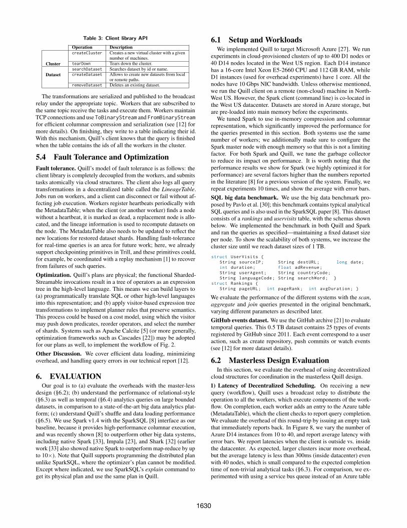
Table 3: Client library API

Operation Description

Cluster

createCluster Creates a new virtual cluster with a givennumber of machines.

tearDown Tears down the cluster.

DatasetsearchDataset Searches dataset by id or name.createDataset Allows to create new datasets from local

or remote paths.removeDataset Deletes an existing dataset.

The transformations are serialized and published to the broadcastrelay under the appropriate topic. Workers that are subscribed tothe same topic receive the tasks and execute them. Workers maintainTCP connections and use ToBinaryStream and FromBinaryStreamfor efficient columnar compression and serialization (see [12] formore details). On finishing, they write to a table indicating their id.With this mechanism, Quill’s client knows that the query is finishedwhen the table contains the ids of all the workers in the cluster.

5.4 Fault Tolerance and OptimizationFault tolerance. Quill’s model of fault tolerance is as follows: theclient library is completely decoupled from the workers, and submitstasks atomically via cloud structures. The client also logs all querytransformations in a decentralized table called the LineageTable.Jobs run on workers, and a client can disconnect or fail without af-fecting job execution. Workers register heartbeats periodically withthe MetadataTable; when the client (or another worker) finds a nodewithout a heartbeat, it is marked as dead, a replacement node is allo-cated, and the lineage information is used to recompute datasets onthe node. The MetadataTable also needs to be updated to reflect thenew locations for restored dataset shards. Handling fault-tolerancefor real-time queries is an area for future work; here, we alreadysupport checkpointing primitives in Trill, and these primitives could,for example, be coordinated with a replay mechanism [1] to recoverfrom failures of such queries.Optimization. Quill’s plans are physical; the functional Sharded-Streamable invocations result in a tree of operators as an expressiontree in the high-level language. This means we can build layers to(a) programmatically translate SQL or other high-level languagesinto this representation; and (b) apply visitor-based expression treetransformations to implement planner rules that preserve semantics.This process could be based on a cost model, using which the visitormay push down predicates, reorder operators, and select the numberof shards. Systems such as Apache Calcite [5] (or more generally,optimization frameworks such as Cascades [22]) may be adoptedfor our plans as well, to implement the workflow of Fig. 2.Other Discussion. We cover efficient data loading, minimizingoverhead, and handling query errors in our technical report [12].

6. EVALUATIONOur goal is to (a) evaluate the overheads with the master-less

design (§6.2); (b) understand the performance of relational-style(§6.3) as well as temporal (§6.4) analytics queries on large boundeddatasets, in comparison to a state-of-the-art big data analytics plat-form; (c) understand Quill’s shuffle and data loading performance(§6.5). We use Spark v1.4 with the SparkSQL [8] interface as ourbaseline, because it provides high-performance columnar execution,and was recently shown [8] to outperform other big data systems,including native Spark [33], Impala [23], and Shark [32] (earlierwork [33] also showed native Spark to outperform map-reduce by upto 10×). Note that Quill supports programming the distributed planunlike SparkSQL, where the optimizer’s plan cannot be modified.Except where indicated, we use SparkSQL’s explain command toget its physical plan and use the same plan in Quill.

6.1 Setup and WorkloadsWe implemented Quill to target Microsoft Azure [27]. We run

experiments in cloud-provisioned clusters of up to 400 D1 nodes or40 D14 nodes located in the West US region. Each D14 instancehas a 16-core Intel Xeon E5-2660 CPU and 112 GB RAM, whileD1 instances (used for overhead experiments) have 1 core. All thenodes have 10 Gbps NIC bandwidth. Unless otherwise mentioned,we run the Quill client on a remote (non-cloud) machine in North-West US. However, the Spark client (command line) is co-located inthe West US datacenter. Datasets are stored in Azure storage, butare pre-loaded into main memory before the experiments.

We tuned Spark to use in-memory compression and columnarrepresentation, which significantly improved the performance forthe queries presented in this section. Both systems use the samenumber of workers; we additionally made sure to configure theSpark master node with enough memory so that this is not a limitingfactor. For both Spark and Quill, we tune the garbage collectorto reduce its impact on performance. It is worth noting that theperformance results we show for Spark (we highly optimized it forperformance) are several factors higher than the numbers reportedin the literature [8] for a previous version of the system. Finally, werepeat experiments 10 times, and show the average with error bars.SQL big data benchmark. We use the big data benchmark pro-posed by Pavlo et al. [30]; this benchmark contains typical analyticalSQL queries and is also used in the SparkSQL paper [8]. This datasetconsists of a rankings and uservisits table, with the schemas shownbelow. We implemented the benchmark in both Quill and Sparkand ran the queries as specified—maintaining a fixed dataset sizeper node. To show the scalability of both systems, we increase thecluster size until we reach dataset sizes of 1 TB.

struct UserVisits {String sourceIP; String destURL; long date;int duration; float adRevenue;String userAgent; String countryCode;String languageCode; String searchWord; }

struct Rankings {String pageURL; int pageRank; int avgDuration; }

We evaluate the performance of the different systems with the scan,aggregate and join queries presented in the original benchmark,varying different parameters as described later.GitHub events dataset. We use the GitHub archive [21] to evaluatetemporal queries. This 0.5 TB dataset contains 25 types of eventsregistered by GitHub since 2011. Each event correspond to a useraction, such as create repository, push commits or watch events(see [12] for more dataset details).

6.2 Masterless Design EvaluationIn this section, we evaluate the overhead of using decentralized

cloud structures for coordination in the masterless Quill design.1) Latency of Decentralized Scheduling. On receiving a newquery (workflow), Quill uses a broadcast relay to distribute theoperation to all the workers, which execute components of the work-flow. On completion, each worker adds an entry to the Azure table(MetadataTable), which the client checks to report query completion.We evaluate the overhead of this round-trip by issuing an empty taskthat immediately reports back. In Figure 8, we vary the number ofAzure D14 instances from 10 to 40, and report average latency witherror bars. We report latencies when the client is outside vs. insidethe datacenter. As expected, larger clusters incur more overhead,but the average latency is less than 300ms (inside datacenter) evenwith 40 nodes, which is small compared to the expected completiontime of non-trivial analytical tasks (§6.3). For comparison, we ex-perimented with using a service bus queue instead of an Azure table

1630

0

100

200

300

400

500

10 20 30 40

Late

ncy

(m

s)

Number of instances

Latency (inside datacenter)

Latency (outside datacenter)

Figure 8: Scheduling overhead;target cluster sizes.

0

0.2

0.4

0.6

0.8

1

0 200 400 600 800 1000

Frac

tio

n w

ith

late

ncy

< L

Latency L (ms)

10 nodes (inside)

10 nodes (outside)

40 nodes (inside)

40 nodes (outside)

Figure 9: Scheduling overhead;inside vs. outside datacenter.

0

200

400

600

800

1000

1200

100 200 300 400

Late

ncy

(m

s)

Number of instances

Figure 10: Scheduling overhead;larger cluster sizes.

0

5000

10000

15000

20000

1 2 3 4 5

Thro

ugh

pu

t (m

sg/s

ec)

Number of Accounts

BroadcastrelayAzure queue

Figure 11: Throughput of cloudstructures.

0

200

400

600

800

1000

1200

1400

10/10GB 20/20GB 30/30GB 40/40GB

Thro

ugh

pu

t (M

illio

n

tup

les/

seco

nd

)

#Nodes/Dataset size

Quill Spark

Figure 12: Scan query with aselectivity of 5%

0

200

400

600

800

1000

1200

1400

10/10GB 20/20GB 30/30GB 40/40GB

Thro

ugh

pu

t (M

illio

n

tup

les/

seco

nd

)

#Nodes/Dataset size

Quill Spark

Figure 13: Scan query with aselectivity of 50%

0

200

400

600

800

1000

1200

1400

10/10GB 20/20GB 30/30GB 40/40GB

Thro

ugh

pu

t (M

illio

n

tup

les/

seco

nd

)

#Nodes/Dataset size

Quill Spark

Figure 14: Scan query with aselectivity of 95%

0

200

400

600

800

1000

1200

1400

1 25 100 200

Exec

uti

on

Tim

e (m

s)

Dataset Replication Factor

scheduling

scan only

Figure 15: Scan latency split-up,varying dataset size

for reporting completion as well, and found the average latency for10 instances to be 340ms within the datacenter (slightly higher thanusing tables). Further, we observe that running the client outside thedatacenter increases latencies by around 70 ms, due to the additionallatency incurred by the distance.2) Effect of Client Location. Figure 8 includes latencies when theclient runs outside the datacenter; we see that average latencies arearound 70ms higher, but are less than 350ms even for 40 nodes. Wenext show the detailed overhead effect when running the user clientoutside vs. inside the datacenter. We use a cluster size of 10 and40 machines, and report the CDF of latencies for inside and outsidedatacenter in Fig. 9. For instance, we note that with 10 (40 resp.)nodes, 85% of latencies are less than 200ms (400ms resp.) whenthe client is inside the datacenter.3) Latency with Larger Cluster Sizes. While we target clusterswith less than 100 machines, we next verify scalability for evenlarger deployments of up to 400 workers. Given a limit on the totalnumber of cores available to us, we use Azure D1 instances with 1core, and vary the number of workers from 100 to 400. Figure 10shows the results from inside the datacenter. We see that latencyoverhead is less than 1 second even with 400 workers, which wouldprovide 44TB of memory if we used D14 instances.4) Throughput of Decentralized Structures. We next measurethe throughput, in terms of number of messages sent and receivedper second, using our cloud structures (Azure queues and broadcastrelay). We use a single client machine with multiple threads tosend and receives messages up to 64 bytes long. Figure 11 showsthroughput as we increase the number of structures to get more par-allelism). We see that even with one structure, we achieve more than1000 messages per second, which is sufficient for our infrequentcoarse-grained control flow messages.

Cloud structures have low latency overhead and high through-put, and can serve as a masterless control flow mechanism.

6.3 Relational Analytical QueriesTo understand the performance and scalability of Quill, we run

the three queries defined in the SQL Big Data Benchmark changingthe selectivity in each case. The dataset size is fixed on a per

node basis to conform the benchmark description. This meansthat we keep around 25 GB (152M rows) of the uservisits dataand 1 GB (18M rows) of the rankings data per node. With thisconfiguration we run the queries in 4 different cluster sizes of 10, 20,30 and 40 nodes, which translates into datasets of 250, 500, 750 and1000 GB respectively. We also run queries with larger data sizesthat, although not specified in the benchmark, helps to understandbetter the performance characteristics of the systems.

6.3.1 Scan Queries1) Scan performance. The first query defined by the benchmark isthe scan shown below, with selectivities of 5%, 50% and 95%.

SELECT pageURL , pageRank FROM RankingsWHERE pageRank > X;

Both systems are columnar and scan only the query predicate col-umn – around 72MB of pageRank data per machine (18M rows ×4 bytes per row). Fig. 12,13, and 14 show the results for Quill andSpark. The throughput in both systems is limited by overheads.

In Quill, with 10 nodes, over 93% of the time is spent on schedul-ing; the total time using a client outside the datacenter is 300ms,while the actual scan takes just 19ms. The overhead is slightly higherthan for an empty query due to additional costs such as client planconstruction, task and metadata serialization, and lineage tracking.The bandwidth of the scan alone (ignoring scheduling overheads)is also low (around 3.8GB/sec) because of the small dataset size.Since scheduling overheads in Quill increase slowly with number ofnodes (see §6.2), scan throughput increases as the cluster grows. Incase of Spark, the overhead is higher, and grows faster with clustersize, preventing its scalability (at 40 nodes, Quill is ∼ 6× faster).2) Scans on larger data. To evaluate performance with non-trivialcompute, we ran additional scan queries with a bigger dataset pernode. We first micro-benchmark Quill by varying the replicationfactor RF of the rankings dataset (each tuple is repeated RF timesto give a rankings dataset size of RF GB per worker. The queryscans RF × 72MB of pageRank data. Figure 15 shows total timeand overhead for 10 workers running the scan, as we vary RF .With RF = 200, we scan 14.4GB of data in 982ms for the scanalone and 1.2secs total including scheduling . As expected, the

1631

0

5

10

15

20

1 25 100 200

Sca

n B

an

dw

idth

(GB

/se

c)

Dataset Replication Factor

scan-only mem. b/w

effective mem. b/w

Figure 16: Scan bandwidth,varying dataset size

0

500

1000

1500

2000

Q1 Q2 Q3

Th

rou

gh

pu

t (M

illi

on

tup

les/

seco

nd

)

Quill Spark

Figure 17: Complex scan queries;varying predicate complexity

0200400600800

10001200140016001800

10/240GB 20/480GB 30/720GB 40/960GB

Th

rou

gh

pu

t (M

illi

on

tup

les/

seco

nd

)

#Nodes/Dataset size

Quill Spark

Figure 18: Aggregate query with2K groups

0200400600800

10001200140016001800

10/240GB20/480GB30/720GB40/960GB

Th

rou

gh

pu

t (M

illi

on

tup

les/

seco

nd

)

#Nodes/Dataset size

Quill Spark

Figure 19: Aggregate query with67K groups

020406080

100120140160180200

10/240GB 20/480GB 30/720GB 40/960GB

Th

rou

gh

pu

t (M

illi

on

tup

les/

seco

nd

)

#Nodes/Dataset size

Quill Spark

Figure 20: Aggregate query with40 million groups

020406080

100120140160180200

10/240GB 20/480GB 30/720GB 40/960GB

Th

rou

gh

pu

t (M

illi

on

tup

les/

seco

nd

)

#Nodes/Dataset size

Quill Spark

Figure 21: Aggregate query with140 million groups

0

100

200

300

400

500

600

10/250GB 20/500GB 30/750GB 40/1TB

Th

rou

gh

pu

t (M

illi

on

tup

les/

seco

nd

)

#Nodes/Dataset size

Quill (shuffle-shuffle)SparkQuill (broadcast-broadcast)Quill (broadcast-shuffle)

Figure 22: Comparison ofdifferent joins; 140M groups

0

100

200

300

400

500

600

10/250GB 20/500GB 30/750GB 40/1TB

Th

rou

gh

pu

t (M

illi

on

tup

les/

seco

nd

)

#Nodes/Dataset size

Quill (shuffle-shuffle)SparkQuill (broadcast-brodcast)Quill (broadcast-shuffle)

Figure 23: Comparison ofdifferent joins; 67K groups

scheduling overhead does not change by much; thus, overhead is alower fraction of total runtime as we increase RF . Figure 16 showsscan bandwidth; as the dataset size increases, overhead is lowerand the scan reaches 15.6GB/sec per worker (11.9GB/sec if weinclude scheduling) for RF = 200. This is respectable because thetheoretical maximum memory bandwidth of 50GB/sec for thesemachines is just around 3.2× our measured scan bandwidth.3) Complex scans. Fig. 17 compares Quill and Spark for three com-plex scans using the uservisits table with 10 workers. Q1 containsan expensive LIKE predicate, where Quill benefits from columnarRegEx matching [15] and achieves throughput 8× higher than Spark.Q2 and Q3 contain 2 and 4 predicates (comparisons and a LIKEpredicate) respectively; Quill is around 4× faster for these queries.

For small data, both systems are dominated by overheads,with Quill scaling better with lower overheads. For larger data,Quill’s scan runs at 15.6GB/sec (11.9GB/sec including schedul-ing). Quill performs better for more complex scans as well.

6.3.2 Grouped Aggregate Queries1) Aggregate performance. The second query of the benchmark isan aggregate query (see below). The query compute the total rev-enue originated per sourceIP. We want to control the complexity ofthe query by modifying the number of groups. To do so, we modifythe length of the sourceIP prefix as suggested in the benchmark. Werun the query with 2K, 67K, 40M and 140M groups.SELECT SUBSTR(sourceIP , 1, 7), SUM(adRevenue)FROM UserVisits GROUP BY SUBSTR(sourceIP , 1, 7);

Executing this query involves a local pre-aggregation, a shuffleacross the network to partition by (sourceIP), and a final aggrega-tion. Thus, the data needed to be communicated across machinesdepends on the number of groups. Interestingly, we found that fora small number of groups (2K and 67K), the best strategy involvesaggregating per-core before re-keying and re-distributing for theglobal shuffle. On the other hand, for larger number of groups,the best strategy ended up being first re-keying and re-distributingacross cores, aggregating, and then shuffling globally. These strate-gies correspond to the query plans of Fig. 1(b) and (d), which areeasily expressed using the ShardedStreamable API (§3). SparkSQLuses the Catalyst optimizer that chooses plans automatically, anddoes not provide users the ability to control or fine-tune the plan asneeded to optimally execute this experiment.

Fig. 18, 19, 20 and 21 show the results for the query for 2K, 67K,40M and 140M respectively. The immediate difference with respectto the scan query is that these graphs show how both Quill and

Spark scale with the cluster size. The reason is that overheads donot dominate the query execution time, and thus more resourceslead to a reduced query completion time.

When the number of groups is small, the amount of data that isrequired to shuffle is small, query time is dominated by the executionof the aggregate function, such as in Fig. 18 and Fig. 19. Quilloutperforms Spark by a factor of 2×, due to the optimized physicalplan, lower scheduling overheads, and higher operator efficiency.As the number of groups increases, shuffling time increases, whichexplains the lower performance in both systems. With a highernumber of groups, the efficiency gains of Quill over Spark broaden,showing an improvement of around 3.5× (see Fig. 20 and Fig. 21).2) Aggregate execution time split-up in Quill. With smaller groupsizes (2K and 67K), execution is CPU-bound by the per-core pre-aggregation because the dataset is highly reduced after that point.For the larger group size (40M groups), different phases of the queryhad different bottlenecks; a run in Quill that took 26secs overallspent 38% on per-core aggregation (CPU-bound), 34.6% on intra-machine shuffle and re-aggregation (memory-bound), 22.6% oninter-machine shuffle (network and serialization-bound), and 4.8%on the final aggregation (CPU-bound).

With efficient group-aggregation over columnar batches, fastnetwork communication, low scheduling overheads, the abilityto fine-tune the physical plan and avoid extra hash computa-tions, Quill can run aggregate queries at high performance.

6.3.3 Join QueriesThe last query of the benchmark is the join query shown below.

The purpose of the query is to calculate the sourceIP and associatedpageRank that gave rise to the highest revenue for a given period oftime, e.g. 1 week. We vary the complexity of this query by changingthe total number of groups according to the sourceIP attribute, as inthe case of the aggregate query.SELECT INTO Temp sourceIP , AVG(pageRank) as avgPageRank ,

SUM(adRevenue) as totalRevenueFROM Rankings AS R, UserVisits AS UVWHERE R.pageURL = UV.destURLAND UV.visitDate BETWEEN Date(’2000 -01 -15’)

AND Date(’2000 -01 -22’)GROUP BY UV.sourceIP;SELECT sourceIP , totalRevenue , avgPageRank FROM TempORDER BY totalRevenue DESC LIMIT 1;

We implement the query using SparkSQL’s physical plan. Thisplan first applies the time-range filter to reduce the UserVisits dataset,after which both datasets are shuffled on the join key, which is inthis case pageURL and destURL. After the shuffle and join, the data

1632

0

5

10

15

20

25

30

Bcast - Bcast Bcast - Shuffle Shuffle - Shuffle

Tim

e (

seco

nd

s)T1 T2 T3 T4 T5

Figure 24: Effect of modifying physical planfor different join strategies

0

200

400

600

800

1 day 1 hour 1 min 1 sec

Th

rou

gh

pu

t (M

illi

on

tup

les/

seco

nd

)

Window size

Quill Spark

Figure 25: Performance of tumbling windowquery for different window sizes

0

200

400

600

800

Th

rou

gh

pu

t (M

illi

on

tup

les/

seco

nd

)

Quill Spark

Figure 26: Performance of hopping windowquery for different window slide/size values

is shuffled again, this time on sourceIP, before running the finalaggregate and top-K. We call this plan shuffle-shuffle to denote thata shuffle occurs across machines and across cores in each machinebefore the join (Fig. 4(a) shows this join strategy).

Fig. 22 and Fig. 23 show the results for the join query when runwith both 140M and 67K groups. For shuffle-shuffle, the perfor-mance of both Quill and Spark is mostly influenced by the timeit takes to transmit the datasets through the network. The slightlybetter throughput of Quill in this case is likely due to more efficientquery processing and data movement.

We then implemented two additional plans for JOIN, that aremore efficient than the one chosen by the Spark query optimizer.We run a strategy called Broadcast-Broadcast, depicted in Fig. 4(b),that does not shuffle the Rankings dataset. Instead, it broadcasts thefiltered UserVisits dataset to all machines in the cluster, and thento each core on each machine. Fig. 22 and Fig. 23 show how thisstrategy is faster than naively shuffling both datasets. However, theperformance of broadcast-broadcast suffers when the dataset sizegrows beyond 750 GB. The reason is that in this strategy, each coreneeds to build a hash table over the entire dataset, which growslinearly with the number of nodes. A better strategy is thereforebroadcast-shuffle, whose plan is depicted in Fig. 4(c). In this case,we perform a broadcast across machines to avoid the expensive shuf-fle of Rankings, but then we perform shuffle both datasets locally,which partitions the hash table across cores, bringing additionalperformance benefits, as shown in Fig. 22 and Fig. 23.

Fig. 24 shows how time is spent in the case of the three join strate-gies. T1 and T2 are the time spent in applying the filter, rekeyingand redistributing the Rankings and UserVisits tables respectively.This clearly shows how shuffling Rankings table is more expensivethan broadcasting UserVisits. T3 is the time spent performing thejoin operation, while T4 is the time spent aggregating page rankand ad revenue per source IP. We see that the broadcast-broadcaststrategy is more expensive due to the higher cost of maintaining ahash table per core. Finally T5 is the time spent on Top-K.

By expressing a large physical plan space, Quill can run joinqueries on large datasets with high performance.

6.4 Temporal Analytical QueriesWe next evaluate temporal queries that compute various grouped

aggregates over tumbling and hopping (sliding) windows, on a clus-ter with 10 machines. We vary the window size, and the slide in caseof hopping windows. We also run the queries on SparkSQL, sincetime is a column in the GitHub schema, to compare performance.1) Tumbling window query. Tumbling windows are easy to expressin SparkSQL, by grouping by the (coarsened) time field. The resultsare shown in Fig. 25. Quill has a performance 3×-4× higher thanSpark. Both systems show a similar behavior for 1 day, 1 hourand 1 min windows. Performance reduces severely in the case of 1second windows for both systems. Quill becomes 2× slower, whileSpark performance drops by a factor of 8. The reasons for this

decrease in performance, however, differ between systems. Quill’sperformance reduces due to the higher amount of data generated, i.e.the bottleneck is not query processing, but data delivery. Since Sparkgroups by time, query processing suffers from a higher number ofgroups created due to the smaller window size.2) Hopping window query. The hopping window query is moredemanding for SparkSQL; while it can leverage the panes trick [24]to implement hopping windows, the number of groups necessary tomaintain grows. We could only run the first three configurations ofthe query, window slide/size of 1 day/1 week, 1 day/1 month, and 1hour/1 week. Other configurations took too long or did not complete,and we do not include them. The results of Fig. 26 show that the costfor Quill does not change—computing a hopping window is similarto a tumbling window, due to native temporal support. Quill’sthroughput is up to 120× higher than Spark (for queries that wewere able to complete on Spark). As before, throughput reduces fora window slide of 1 second due to the cost of delivering results.

By carefully layering a temporal library and adding efficientReKey, ReDistribute, and time-ordered merge operations, Quillcan process temporal queries very efficiently.

6.5 Shuffle and Data Loading PerformanceWe often need to process raw data in timestamp order by key, for

example, to detect sequential patterns in the data. Such queries maynot benefit from pre-aggregation, resulting in the need to shuffle theraw data. We generate a synthetic dataset with two random longfields, and execute a Broadcast and a shuffle (ReKey+ReDistribute)query (across all machines). For broadcast, we found the actualshuffle throughput (incoming plus outgoing) to reach 9.79 Gbpsper node on a 40-machine cluster, which is close to the 10 GbpsNIC bandwidth limit. Shuffle additionally involves computing hashvalues and moving data by hash bucket before sending it on the wire;we achieve an effective throughput of 8.35 Gbps per node. Notethat users could also materialize datasets after a ReKey to leveragepre-computed keys and hash values.

Next, we measure the performance of loading a 762GB comma-separated text dataset with 16 fields, stored across 8 Azure storageaccounts. With 40 cloud workers, we load the data is 85secs, withan average read throughput of around 9 Gbps per storage account,close to the enforced limit of 10 Gbps per storage account.

7. RELATED WORKIn Section 1.1 and Table 1, we covered today’s analytics platforms

in terms of satisfying our target requirements; more details follow.Databases & big data systems. DBMSs compile SQL queries intoplans with high performance, but the plans cannot be modified,programmed, or transferred to real-time. They lack temporal opera-tor support or deep integration into the HLL type-system. Beyondbroadcast and exchange operators, commercial DBMSs do not of-fer more complex data-dependent duplication strategies for datamovement. As Fig. 2 shows, Quill offers an alternative to query

1633

hinting that allows users to control and validate their plans, or pro-gram them directly in a HLL. By making it easy for optimizersto express and execute plans, we expect to see the growth of HLLoptimizer libraries that target specific verticals or scenarios as well.Systems such as map-reduce [19] and Spark RDDs [33] expose akeyed computation model to exploit data-parallelism, but are unableto express and optimize for the rich space of distributed executionstrategies we target. These systems also expose SQL front-endssuch as Hive [31] that have limitations as discussed in Section 1. Incontrast, Quill separates query logic, data movement, and logicalkeying to allow the expression of a rich space of physical plans thatimplement complex temporal logic and are transferable to real-timeas well. Moreover, existing systems implement a master-workerarchitecture unlike Quill, which uses decentralized cloud structuresfor client-driven coordination.Streams & Physical Algebras. Single-node streaming systems [9,15] have rich query models but are inadequate to meet high datavolumes and scale. Streaming systems such as Storm [7], Flink [4],MillWheel [2], and Google Cloud Dataflow [3] expose a fine-grainedAPI using which users can process and produce 〈key, value〉 pairs,with richer temporal APIs on top. As discussed in §3.3.2, the fine-grained API results in several inefficiencies at the data plane. Incontrast, Quill provides functional transformations such as ReKey,ReDistribute, and Multicast that are executed at the data plane inbatched columnar form by exploiting white-box lambda expressionparameters and code generation. Dryad’s physical algebra is anarbitrary graph which cannot be programmed, unlike Quill whichexposes a small, readable, and powerful set of functional transforma-tions to specify physical plans. DryadLINQ and SparkSQL operateat the logical specification level like databases, and users cannottweak physical plans. Quill’s physical algebra explicitly separatesdata movement from keying, and adds new data movement func-tions beyond ReDistribute that expand query expressiveness withoutgiving up on performance. Further, existing systems do not supportprimitives to optimize inter-node vs. intra-node plans. Finally, theseparation of Query as a layer allows temporal logic specification(leveraging Trill) independent from dataflow specification, guar-anteeing transferability without loss of performance, by exposingbatching and grouping to the innermost loop.

8. CONCLUSIONSQuill is a library and distributed platform for analytics over large

datasets. We propose a new abstraction called ShardedStreamable,that can express efficient distributed physical query plans that aretransferable between real-time and offline deployments Sharded-Streamable decouples incremental query logic specification, datamovement, and keying; this allows Quill to express a broad spaceof plans with complex querying functionality, while leveraging tem-poral libraries such as Trill. Quill’s layered architecture provides aseparation of responsibilities with independently useful components,while retaining high performance. We built Quill for the cloud, witha master-less design that leverages off-the-shelf distributed compo-nents found in cloud providers. Experiments on up to 400 cloudmachines, on benchmark and real datasets up to 1TB, find Quillto incur low overhead and outperform SparkSQL by up to orders-of-magnitude for temporal and 6× for relational queries, whilesupporting significantly expanded temporal querying functionality.Acknowledgments. We would like to thank Mike Barnett, TysonCondie, Ravi Ramamurthy, James F. Terwilliger, Markus Weimer,and the anonymous reviewers for their comments, help, and support.

9. REFERENCES[1] D. J. Abadi et al. The Design of the Borealis Stream

Processing Engine. In CIDR, 2005.[2] T. Akidau et al. MillWheel: Fault-Tolerant Stream Processing

at Internet Scale. In VLDB, 2013.[3] T. Akidau et al. The Dataflow Model: A Practical Approach to

Balancing Correctness, Latency, and Cost in Massive-Scale,Unbounded, Out-of-Order Data Processing. In VLDB, 2015.

[4] A. Alexandrov et al. The Stratosphere Platform for Big DataAnalytics. The VLDB Journal, 23(6):939–964, Dec. 2014.

[5] Apache. Calcite. http://calcite.apache.org.[6] Apache Kafka. http://kafka.apache.org/.[7] Apache Storm. http://storm.apache.org/.[8] M. Armbrust et al. Spark SQL: Relational Data Processing in

Spark. In SIGMOD, 2015.[9] B. Babcock, S. Babu, M. Datar, R. Motwani, and J. Widom.

Models and issues in data stream systems. PODS, 2002.[10] S. Blanas et al. A comparison of join algorithms for log

processing in mapreduce. In SIGMOD, 2010.[11] N. Bruno, S. Chaudhuri, and R. Ramamurthy. Power hints for

query optimization. In ICDE, 2009.[12] B. Chandramouli et al. The Quill Distributed Analytics

Library and Platform. Technical report, Microsoft Research(MSR-TR-2016-25). http://aka.ms/quill-tr.

[13] B. Chandramouli et al. StreamRec: A Real-TimeRecommender System. 2011.

[14] B. Chandramouli et al. Scalable Progressive Analytics on BigData in the Cloud. In VLDB, 2014.

[15] B. Chandramouli et al. Trill: A High-performanceIncremental Query Processor for Diverse Analytics. Proc.VLDB Endow., 8(4):401–412, Dec. 2014.

[16] B. Chandramouli, J. Goldstein, and S. Duan. TemporalAnalytics on Big Data for Web Advertising. In ICDE, 2012.

[17] S. Chu et al. From Theory to Practice: Efficient Join QueryEvaluation in a Parallel Database System. In SIGMOD, 2015.

[18] Cloudera Engineering Blog. Cloudera Impala: Real-TimeQueries in Apache Hadoop, For Real.http://tinyurl.com/bsrhcf7.

[19] J. Dean and S. Ghemawat. MapReduce: Simplified DataProcessing on Large Clusters. In CACM, 2008.

[20] Forcing Query Plans in SQL Server. http://aka.ms/etgyp4.[21] GitHub Archive. https://www.githubarchive.org/.[22] G. Graefe. The Cascades Framework for Query Optimization.

Data Engineering Bulletin, 18, 1995.[23] M. Kornacker et al. Impala: A modern, open-source SQL

engine for Hadoop. In CIDR, 2015.[24] J. Li et al. No Pane, No Gain: Efficient Evaluation of

Sliding-window Aggregates over Data Streams. SIGMODRec., 2005.

[25] N. Marz. How to beat the CAP theorem.http://tinyurl.com/3lqwebc.

[26] Expression Trees in .NET.https://msdn.microsoft.com/en-us/library/bb397951.aspx.

[27] Microsoft Azure. https://azure.microsoft.com/en-us/.[28] A. Okcan and M. Riedewald. Processing Theta-Joins using

MapReduce. In SIGMOD, 2011.[29] Oracle9i Database Performance Tuning Guide and Reference.

Using Explain Plan. http://tinyurl.com/hkh7zx6.[30] A. Pavlo et al. A comparison of approaches to large-scale data

analysis. In SIGMOD, 2009.[31] A. Thusoo et al. Hive - A Warehousing Solution Over a

Map-Reduce Framework. VLDB, 2009.[32] R. S. Xin, J. Rosen, et al. Shark: SQL and Rich Analytics at

Scale. In SIGMOD, 2013.[33] M. Zaharia et al. Resilient Distributed Datasets: A

Fault-Tolerant Abstraction for In-Memory Cluster Computing.In NSDI, 2012.

1634