queueing theory with applications and … theory with applications and special consideration to...

QUEUEING THEORY WITH APPLICATIONS AND SPECIAL

CONSIDERATION TO EMERGENCY CARE

JAMES KEESLING

1. Introduction

Much that is essential in modern life would not be possible without queueing theory. All com-munication systems depend on the theory including the Internet. In fact, the theory was developedat the time that telephone systems were growing and requiring more and more sophistication tomanage their complexity. Much of the theory was developed by Agner Krarup Erlang (1878-1929).He worked for Copenhagen Telephone Company. His contributions are widely seen today as funda-mental for how the theory is understood and applied. Those responsible for the early developmentof what has become the Internet relied on the work of Erlang and others to guide them in designingthis new system. Leonard Kleinrock was awarded the National Medal of Honor for his pioneer-ing work leading to the Internet. His book [7] reworked Queueing Theory to apply to this newdeveloping technology.

These notes are being compiled from a seminar in the Department of Mathematics at the Uni-versity of Florida on Queueing Theory Applied to Emergency Care. The seminar meets weekly andthe material is updated based on the presentations and discussion in the seminar. In the notes anattempt is made to introduce the theory starting from first principles. We assume some degree offamiliarity with probability and density functions. However, the main distributions and conceptsare identified and discussed in the notes along with some derivations. We will try to develop intu-ition as well. Often the intuition is gained by reworking a formula in a way that the new versionbrings insight into how the system is affected by the various parameters.

If one makes complete rigor the principal goal in Mathematics, then the subject can becomeextremely dry. We will be content to be sure that the results are correct and any argumentselucidating. We will focus on the insights that might be relevant to the various applications thatwe have in mind.

We will first introduce Poisson processes. This forms the basic underpinning of elementaryqueueing theory. Next we will introduce the simple queue. This is a queueing system with asingle server with Poisson arrivals and exponential service times. We then discuss more complexqueueing systems. As we introduce new ideas we will try to give applications and hint how the ideaswill apply to emergency care. The general applications will range from telephone communicationsto stochastic modeling of population dynamics and other biological systems. The most complexqueueing systems are frequently beyond mathematical analysis. This is likely the case for a realisticmodel of emergency care. Such cases will be studied by simulation. The tools of simulation willbe gradually developed through the notes. One of the major accomplishments of the seminar is arealistic model of the flow of patients in the emergency room.

1

2 JAMES KEESLING

There are several texts that we recommend on the subject of queueing theory. The book byDonald Gross, John Shortle, James Thompson, and Carl Harris, Fundamentals of Queueing The-ory [5] is recommended for those involved in this project. Some others that may be consulted areProbability, Markov Chains, Queues, and Simulation: the Mathematical Basis of Performance Mod-eling by William Stewart [9], An Introduction to Queueing Theory and Matrix-Analytic Methodsby Lothar Breuer and Dieter Baum [2], Queueing Theory and Telecommunications: Networks andApplications by Giovanni Giambene [4], Optimal Design of Queueing Systems by Shaler Sticham,Jr. [6], and Elements of Queueing Theory, Palm Martingale Calculus and Stochastic Recurrencesby Francois Baccelli and Pierre Bremaud [1]. Efficiency and reduced waiting times are only part ofthe management concerns of emergency care. A valuable general guide to operational improvementfor emergency departments is given in [3].

As mentioned, this material is compiled from a seminar that meets regularly to study the subjectof Queueing Theory Applied to Emergency Care. Here is a picture of the participants at our meetingon October 25, 2012.

Figure 1. Emergency Care/Queueing Seminar: (Left to Right) Jed Keesling,Trent Register, Joshua Hurwitz, Jean Larson, James Maissen, Hayriye Gulbu-dak, Evan Milliken, Jo Ann Lee, David Zhou, Scott McKinley, Lou Block, AdrianTyndall (Head of Emergency Services at Shands)

2. Poisson Processes

Randomness is hard to recognize. If points are thought to be random on a line or in the plane,then we would be suspicious if the points were regular distances apart. On the other hand, if thepoints are truly random and independent, then there will appear to be clustering. We will see whythis is so when we cover exponential waiting times in the next section. Arrivals in queueing theoryare assumed to be random and independent, but at some given rate. This is a Poisson process. Wefirst give the axioms for a Poisson process which intuitively describe a process in which the eventsare random and independent. In the following let α > 0 be a real constant.

Definition 2.1. A Poisson process is a random sequence of events such that the following threeaxioms hold.

(1) The probability of an event occurring in a small interval of time ∆t is given by

Pr = α ·∆t+ o(∆t).

QUEUEING THEORY WITH APPLICATIONS AND SPECIAL CONSIDERATION TO EMERGENCY CARE 3

(2) If I and J are disjoint intervals, then the events occurring in them are independent.

(3) The probability of more than one event occurring in an interval ∆t is o(∆t2

).

From these axioms one can derive properties of the distribution of events. The first formula wewill derive is the probability of exactly k events occurring in an interval of length t. To derive theformula we divide the interval into n equal subintervals each of length t

n . For large enough n, the

probability of an event in each of these intervals is approximately αtn . The probability that an event

will not occur in a particular subinterval is 1− αtn . Thus, the binomial probability for k occurrences

is given by

B(n, k) =

(nk

)(αt

n

)k·(

1− αt

n

)n−k.

Using the fact that limn→∞(1 + a

n

)n= ea one can easily calculate the limit of the above.

limn→∞

B(n, k) =(αt)k

k!exp(−αt)

This calculation tells us the probability of k occurrences in an interval of length t. The proba-bilities for k = 0, 1, 2, . . . give a Poisson distribution. The average number in the interval is k = αtand the variance is σ2 = αt. For large αt this is approximately a normal distribution. Below is agraph of the Poisson distribution for αt = 5, 10, and 20.

Ê

Ê

Ê

Ê

Ê Ê

Ê

Ê

Ê

Ê

ÊÊÊ Ê Ê Ê Ê Ê Ê Ê Ê Ê Ê Ê Ê Ê Ê Ê Ê Ê Ê‡ ‡ ‡

‡

‡

‡

‡

‡

‡

‡ ‡

‡

‡

‡

‡

‡

‡‡‡ ‡ ‡ ‡ ‡ ‡ ‡ ‡ ‡ ‡ ‡ ‡ ‡Ï Ï Ï Ï Ï Ï Ï Ï Ï Ï

Ï ÏÏÏÏÏÏÏÏ Ï Ï Ï

ÏÏÏÏÏÏÏÏ Ï

5 10 15 20 25 30

0.05

0.10

0.15

Figure 2. Poisson Distributions

3. Exponential Waiting Times

A Poisson process is equivalent to points being placed on a line by a stochastic process suchthat the distribution of distances between the points are independent from the density functionα exp(−αt). If we think of the line as being time and the events as occurring at certain times, thedensity function is called the exponential waiting time with rate α or average waiting time 1

α . The

average waiting time for this density function is 1α and the variance is 1

α2 .Suppose that we have a Poisson process as described in §2. Suppose that we want to know the

density function for the time to the next event. What is the probability that the next event willoccur between t and t + ∆t? For the time T to the next event to lie between t and t + ∆t, there

4 JAMES KEESLING

must not be an event in the interval [0, t]. This is the probability of 0 events in the interval of

length t which is (αt)0

0! exp(−αt) = exp(−αt). In addition, there must be an event in the interval[t, t+∆t]. The probability of this is approximately α∆t. So, by the independence of events in thesetwo intervals, the probability that both would occur is approximately α∆t · exp(−αt). Dividing by∆t and taking the limit leads us to the density function, α exp(−αt). So, a Poisson process hasexponential waiting times. It is easy to show that these are independent since events in disjointintervals are independent.

On the other hand, it can also be shown that if we have independent exponential waiting timesbetween events, it will be a Poisson process. It is a good test of your understanding to prove this.

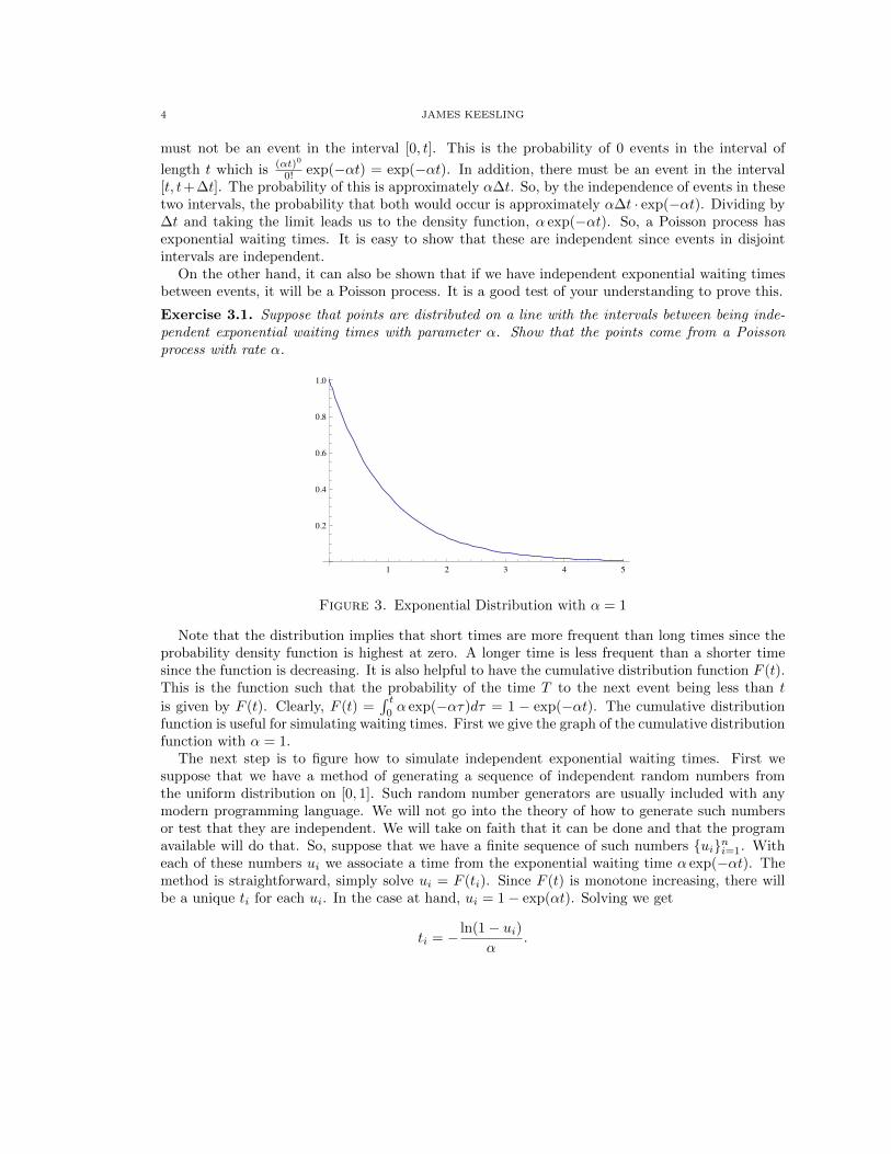
Exercise 3.1. Suppose that points are distributed on a line with the intervals between being inde-pendent exponential waiting times with parameter α. Show that the points come from a Poissonprocess with rate α.

1 2 3 4 5

0.2

0.4

0.6

0.8

1.0

Figure 3. Exponential Distribution with α = 1

Note that the distribution implies that short times are more frequent than long times since theprobability density function is highest at zero. A longer time is less frequent than a shorter timesince the function is decreasing. It is also helpful to have the cumulative distribution function F (t).This is the function such that the probability of the time T to the next event being less than t

is given by F (t). Clearly, F (t) =∫ t0α exp(−ατ)dτ = 1 − exp(−αt). The cumulative distribution

function is useful for simulating waiting times. First we give the graph of the cumulative distributionfunction with α = 1.

The next step is to figure how to simulate independent exponential waiting times. First wesuppose that we have a method of generating a sequence of independent random numbers fromthe uniform distribution on [0, 1]. Such random number generators are usually included with anymodern programming language. We will not go into the theory of how to generate such numbersor test that they are independent. We will take on faith that it can be done and that the programavailable will do that. So, suppose that we have a finite sequence of such numbers {ui}ni=1. Witheach of these numbers ui we associate a time from the exponential waiting time α exp(−αt). Themethod is straightforward, simply solve ui = F (ti). Since F (t) is monotone increasing, there willbe a unique ti for each ui. In the case at hand, ui = 1− exp(αt). Solving we get

ti = − ln(1− ui)α

.


1 2 3 4 5

0.2

0.4

0.6

0.8

1.0

Figure 4. Cumulative Distribution of the Exponential Distribution with α = 1

Since 1−ui also comes from a uniform distribution on [0, 1], we could replace 1−ui by ui in the

formula. Doing so would reduce the computation by one floating point operation: ti = − ln(ui)α .

Figure 5 gives a randomly generated list of twenty random numbers ui followed by the associatedexponential waiting times with α = 1.

Figure 5. Twenty Independent Exponential Waiting Times with α = 1

6 JAMES KEESLING

Figure 6. Twenty Independent Samples from 1π ·

11+x2


Figure 7. Mathematica Program for Poisson Simulation

8 JAMES KEESLING

4. Independent Numbers from an Arbitrary Distribution

In the derivation and simulation in the last section, the distribution that we were using wasthe exponential distribution with probability density function p(t) = α exp(αt) and cumulativedistribution function F (t) = 1 − exp(αt). However, if we wanted to generate a set of independentrandom numbers from an arbitrary probability density function, p(t), we would go through thesame process using its cumulative distribution function F (t). We would use a set of independentrandom numbers from the uniform distribution on [0, 1], {ui}Ni=1, and then solve for {xi}Ni=1 usingthe equation ui = F (xi).

For example, suppose that our probability density function is p(x) = 1π ·

11+x2 . Then the cumula-

tive distribution is F (x) = 1π · arctan(x). As before we generate twenty independent numbers from

this distribution using random numbers from [0, 1]. Figure 5 gives a list numbers generated fromthis distribution.

In the next few sections, we will assume exponential exponential waiting times. The reason isto be able to make certain calculations. When we derive the Kolmogorov-Chapman differentialequations, we need the processes to only depend on the most recent state. This is called the Markovproperty for a stochastic process. If the waiting time to leave a given state is exponential, then theMarkov property will be satisfied. When this assumption is not appropriate, we may have to resortto simulation. So, the ability to generate independent values from a general distribution will bevaluable tool.

Figure 6 is a program in Mathematica that simulates a Poisson process. The plot is n(t) thenumber of events that have occurred in the interval [0, t]. In the simulation, we generate a table ofindependent exponential waiting times. We use these times as the times between successive eventsin the Poisson process. The output of the various computations in the simulation are shown tomake the program more transparent. In Mathematica one could have hidden this output. Later inthis document we will be simulating much more complex examples. In the program one can changethe number of events n and the rate α.

What are examples of Poisson processes? Radioactive decay is one example. If you take thetransformation of one of the atoms in the radioactive sample as an event, then the sequence ofthese decays will be a Poisson process. In telephone networks one generally assumes that a customertrying to make a call is an event. It is assumed that this is a Poisson process and this assumptionis supported in practice. Of course, the rate α will change with the time of day and day of theweek. We will be assuming that α is constant, but it is not hard to analyze the case that α is timedependent. The arrival of information packets at a given node in the Internet is assumed to bePoisson. The distances between successive cars in a lane on a highway are sometimes assumed tobe independent and exponential.

We can also derive a theory of Poisson processes for events in the plane or space. How wouldyou modify the axioms in these cases? How would the properties that we derived change in thesesettings? Can you think of a way of simulating a Poisson process in a region of the plane? In threespace? In Rn?

An example of a Poisson process in the plane would be the location of a species of plant whoseseeds disperse widely from the parent plant. The location of stars in a star chart down to a givenmagnitude will be Poisson. The three dimensional location of stars is Poisson. However, the densityα varies through space.


Figure 8. The von Koch Curve

Figure 9. The Sierpinski Carpet

Figure 10. The Menger Sponge

10 JAMES KEESLING

One can also define Poisson processes on fractal sets or other spaces having a regular measure.What do you think would be a good definition? How could you simulate such a Poisson process onthe von Koch curve, the Sierpinski carpet, or the Menger sponge? Figures 8, 9, and 10 give picturesof these objects if you are not familiar with them.

5. A Simple Queue

In this section we explain a simple queue. This will illustrate the fundamentals of the theory.There are a number of good references for queueing theory. We recommend Fundamentals ofQueueing Theory by Donald Gross, John Shortle, James Thompson, and Carl Harris [5].

A simple queue has a single server that can serve one customer at a time. The service time isan exponential waiting time with parameter σ. The service times are assumed to be independentand independent of arrivals. The arrival rate is Poisson with rate α. If a customer arrives and theserver is occupied, that customer goes to the end of the waiting line. Customers are served in orderof arrival.

There is a notation that has become common in the field that communicates the assumptionsbeing made about a given queueing system. The case described above is denoted M/M/1/FIFO.The first M indicates the assumption about arrivals. In this case they are Markovian (Poisson).The second M indicates the assumption about the service times, that they are exponential waitingtimes. The third indicator gives the number of servers. The last indicates the queueing discipline,that is in what order the waiting customers are served. FIFO indicates that they are served in theorder “first in first out”.

There are also some helpful diagrams that are used to describe this queue. In the one thatfollows, the clients are denoted by circles and the service facility by a box. The circle in the boxdenotes the client that is being served by that server.

!

! !!

Figure 11. Diagram of a Simple Queue

We will let the states of the system at a given time to be the number of customers that havearrived and not completed service. The state n will be in the set {0, 1, 2, . . . }. If the state is n > 0,then one customer is being served and n− 1 are waiting in line. We can also represent the systemin the following way.

We can also represent this type of queue with the following diagram.

0α−→←−σ

1α−→←−σ

3α−→←−σ

· · ·nα−→←−σ

n+ 1 · · ·

Let pn(t) denote the probability that the system is in state n at time t. We will be assuming a setof initial probabilities {pn(0)}∞n=0. We will now describe a set of differential equations that governthe system, the Kolmogorov-Chapman equations. Suppose that we have the following probabilitiesat time t, {pn(t)}∞n=0. How can these change in a small interval of time ∆t? Consider the casen = 0.

p0(t+ ∆t) ≈ σ∆t · p1(t) + (1− α∆t) · p0(t)


This leads to the differential equation.

dp0(t)

dt= σp1(t)− αp0(t)

Similarly we can derive a differential equation for each n > 0.

dpn(t)

dt= σpn+1 + αpn−1(t)− (α+ σ)pn(t)

The system of differential equations determines the behavior of the probabilities through timeafter a time t that the values {pn(t)}∞n=0 are known.

If σ > α, we can expect that these probabilities will have a limiting value. We call the set ofthese limiting values the steady-state for the system. We can solve for the steady-state by settingthe derivatives equal to zero in the Kolmogorov-Chapman equations. In the case of a simple queuewith σ > α, this leads to the following probabilities.

pn =(ασ

)n·(

1− α

σ

)The average number in the system E(n) = n can be calculated.

n =ασ

1− ασ

Consider a simple example. Suppose that α = 9. This could be nine customer arrivals per hourif the unit of time is an hour. Suppose that σ = 10. At first glance it would seem that this queueingsystem should run smoothly. In an hour we would expect nine arrivals. The server could handleten in the hour. So, he should be able to finish the work and have time for a rest before the nexthour. However, this naıve analysis does not take proper account of the randomness of the process.The formula for n above shows that the average number in the system is

n =910

1− 910

= 9.

This is much more congested than one would have imagined. A customer arriving at a timewhen the system is in steady-state would fine nine customers already in the system and would haveto wait on average ten times as long as one service time 1

σ = 110 , that is, the average wait would be

one hour rather than just six minutes.Let us imagine that this is an approximate of emergency care and a typical time of treatment is

one hour. Then σ = 1 and α = 910 . We have changed the time scale, but this does not change the

ratio between α and σ which is still 910 . So, n = 9 and the average time that the patient will be in

the emergency care facility is a total of ten hours, ten times as long as the treatment period of onehour.

What this demonstrates is that it is important to have an accurate model of how randomness isaffecting the system. If we have not properly taken it into account, the congestion that arises dueto randomness will be unexpected and may be overwhelming. In what follows we will be showingthat the congestion that is due to randomness can be lowered to a manageable level by a modestadditional investment of resources.

12 JAMES KEESLING

6. A. K. Erlang

Historically, Agner Krarup Erlang (1878 - 1929) developed queueing theory to analyze telephonesystems. He worked for Copenhagen Telephone Company during the period that telephone systemswere growing in complexity. Obviously, randomness is an integral part such a system. WhenARPANET was being considered, the pioneers of this precursor of the Internet used the queueingtheory advanced by Erlang and others to show that the system was feasible. One of those involvedin those early days was Leonard Kleinrock [7]. Figure 13 shows him receiving the National Medalof Honor for his pioneering work leading to the Internet. Queueing theory continues to play a vitalrole in analyzing the functioning of the Internet. Figure 12 is a picture of Erlang available fromWikimedia Commons.

Figure 12. Agner Krarup Erlang


Figure 13. Leonard Kleinrock Receiving the National Medal of Honor

7. Queue with an Infinite Number of Servers

In practice we will have a finite number of servers. However, in order to determine how manyservers will be adequate, it makes sense to assume an infinite number of servers and see if this mightbe helpful in determining what finite number of servers might be adequate. Since every arrival willhave a server available, there will be no waiting line for this system. We will continue to assumePoisson arrivals at a rate α and exponential waiting times with parameter σ. The system can bedescribed in our queueing shorthand as M/M/∞. Below is a diagram of this type of queueingsystem.

The states of the system are {n = 0, 1, 2, . . . }. However, now the rates are different as representedby the following diagram.

0α−→←−σ

1α−→←−2·σ· · ·

α−→←−

(n−1)·σn− 1

α−→←−n·σ

nα−→←−

(n+1)·σn+ 1 · · ·

The steady-state probability of being in each state n is given by the following formula.

pn =

(ασ

)nn!· e−ασ

So, we see the Poisson distribution again, this time in the context of a queueing system with aninfinite number of servers.

In applications to communication systems and the Internet, ασ will be large. In that case, the

Poisson distribution will be approximately normal with mean µ = ασ and variance σ2 = α

σ . In

14 JAMES KEESLING

!!

α !

σ !

σ !

σ !

σ !

σ !

σ !

σ !

σ !

!

Figure 14. Diagram of Queue with an Infinite Number of Servers

practice n will have to be finite. If we choose n to be several, say k, standard deviations beyondthe mean α

σ , then it will be rare that there are more clients than servers.

n =α

σ+ k ·

√α

σ

Exercise 7.1. Suppose that in a certain town there are 200, 000 land-line telephones. Suppose thatthese are used on average seven times per day and each use is equally likely at any time of the day.Assume that the average time of use each time is five minutes and that this is given by an exponentialwaiting time. Assume that it is unacceptable for there to be greater than 1

1,000,000,000 proportion of

the time that a telephone connection cannot be made. If you were designing the system, what shouldbe the capacity for the number of connections in the system?

Exercise 7.2. The number of erythrocytes in the human body is approximately 2− 3× 1013. Theerythrocytes do not reproduce in the human body and have a life-span of approximately 100-120days. These cells are produced in bone marrow through a process known as erythropoiesis and thenreleased into the bloodstream. How many erythrocytes are made each day? How long could a personsurvive if the erythropoietic system were to shut down completely. Assume that a person could barelysurvive with 10% of the normal level of erythrocytes.

8. Queues with a Finite Number of Servers

Now suppose that there are a finite number of servers. Perhaps that finite number was chosen bythe method in the last paragraph of the last section, but we can derive the Kolmogorov-Chapmanequations and the steady-state probabilities without knowing just how the number was determined.Let us suppose the there are m servers and that any time the system has more than n > m clients,


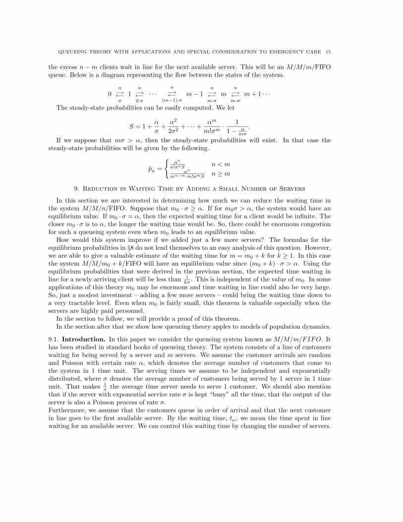
the excess n−m clients wait in line for the next available server. This will be an M/M/m/FIFOqueue. Below is a diagram representing the flow between the states of the system.

0α−→←−σ

1α−→←−2·σ· · ·

α−→←−

(m−1)·σm− 1

α−→←−m·σ

mα−→←−m·σ

m+ 1 · · ·

The steady-state probabilities can be easily computed. We let

S = 1 +α

σ+

α2

2σ2+ · · ·+ αm

m!σm· 1

1− αmσ

.

If we suppose that mσ > α, then the steady-state probabilities will exist. In that case thesteady-state probabilities will be given by the following.

pn =

{αn

n!σnS n < mαn

mn−m·m!σmS n ≥ m

9. Reduction in Waiting Time by Adding a Small Number of Servers

In this section we are interested in determining how much we can reduce the waiting time inthe system M/M/n/FIFO. Suppose that m0 · σ ≥ α. If for m0σ > α, the system would have anequilibrium value. If m0 · σ = α, then the expected waiting time for a client would be infinite. Thecloser m0 · σ is to α, the longer the waiting time would be. So, there could be enormous congestionfor such a queueing system even when m0 leads to an equilibrium value.

How would this system improve if we added just a few more servers? The formulas for theequilibrium probabilities in §8 do not lend themselves to an easy analysis of this question. However,we are able to give a valuable estimate of the waiting time for m = m0 + k for k ≥ 1. In this casethe system M/M/m0 + k/FIFO will have an equilibrium value since (m0 + k) · σ > α. Using theequilibrium probabilities that were derived in the previous section, the expected time waiting inline for a newly arriving client will be less than 1

kσ . This is independent of the value of m0. In someapplications of this theory m0 may be enormous and time waiting in line could also be very large.So, just a modest investment – adding a few more servers – could bring the waiting time down toa very tractable level. Even when m0 is fairly small, this theorem is valuable especially when theservers are highly paid personnel.

In the section to follow, we will provide a proof of this theorem.In the section after that we show how queueing theory apples to models of population dynamics.

9.1. Introduction. In this paper we consider the queueing system known as M/M/m/FIFO. Ithas been studied in standard books of queueing theory. The system consists of a line of customerswaiting for being served by a server and m servers. We assume the customer arrivals are randomand Poisson with certain rate α, which denotes the average number of customers that come tothe system in 1 time unit. The serving times we assume to be independent and exponentiallydistributed, where σ denotes the average number of customers being served by 1 server in 1 timeunit. That makes 1

σ the average time server needs to serve 1 customer. We should also mentionthat if the server with exponential service rate σ is kept “busy” all the time, that the output of theserver is also a Poisson process of rate σ.Furthermore, we assume that the customers queue in order of arrival and that the next customerin line goes to the first available server. By the waiting time, tω, we mean the time spent in linewaiting for an available server. We can control this waiting time by changing the number of servers.

16 JAMES KEESLING

9.2. Estimated waiting time formula. The estimated waiting time formula is reached by usingPoisson probabilities and can be found in the standard books of queueing theory, as [?], but we willderive it here again, to make everything clear and the future proofs more understandable.

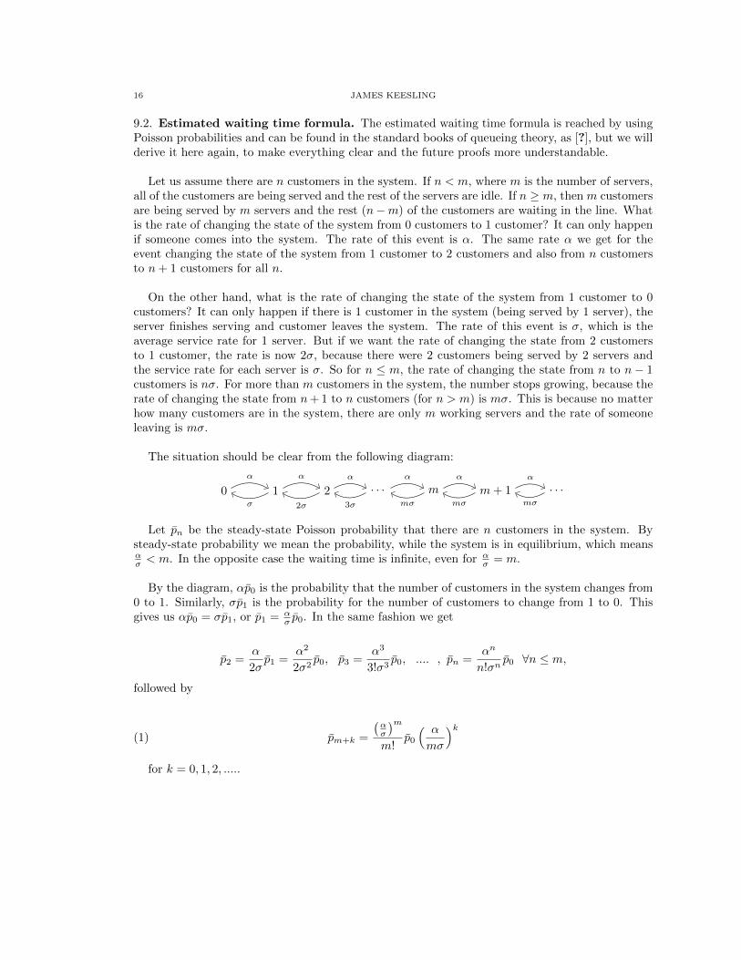
Let us assume there are n customers in the system. If n < m, where m is the number of servers,all of the customers are being served and the rest of the servers are idle. If n ≥ m, then m customersare being served by m servers and the rest (n−m) of the customers are waiting in the line. Whatis the rate of changing the state of the system from 0 customers to 1 customer? It can only happenif someone comes into the system. The rate of this event is α. The same rate α we get for theevent changing the state of the system from 1 customer to 2 customers and also from n customersto n+ 1 customers for all n.

On the other hand, what is the rate of changing the state of the system from 1 customer to 0customers? It can only happen if there is 1 customer in the system (being served by 1 server), theserver finishes serving and customer leaves the system. The rate of this event is σ, which is theaverage service rate for 1 server. But if we want the rate of changing the state from 2 customersto 1 customer, the rate is now 2σ, because there were 2 customers being served by 2 servers andthe service rate for each server is σ. So for n ≤ m, the rate of changing the state from n to n − 1customers is nσ. For more than m customers in the system, the number stops growing, because therate of changing the state from n+ 1 to n customers (for n > m) is mσ. This is because no matterhow many customers are in the system, there are only m working servers and the rate of someoneleaving is mσ.

The situation should be clear from the following diagram:

0 1 2 · · · m m+ 1 · · ·α

σ

α

2σ

α

3σ

α

mσ

α

mσ

α

mσ

Let pn be the steady-state Poisson probability that there are n customers in the system. Bysteady-state probability we mean the probability, while the system is in equilibrium, which meansασ < m. In the opposite case the waiting time is infinite, even for α

σ = m.

By the diagram, αp0 is the probability that the number of customers in the system changes from0 to 1. Similarly, σp1 is the probability for the number of customers to change from 1 to 0. Thisgives us αp0 = σp1, or p1 = α

σ p0. In the same fashion we get

p2 =α

2σp1 =

α2

2σ2p0, p3 =

α3

3!σ3p0, .... , pn =

αn

n!σnp0 ∀n ≤ m,

followed by

(1) pm+k =

(ασ

)mm!

p0

( α

mσ

)kfor k = 0, 1, 2, .....


The sum of all possible probabilities must be equal to 1, which gives us equality

1 =

∞∑k=0

pk = p0

(1 +

α

σ+

α2

2σ2+ ....+

(ασ

)mm!

(1 +

α

mσ+( α

mσ

)2+ ....

)).

The expression in the last bracket is a geometrical series, so we can write

(2) p0 =1

S, where S = 1 +

α

σ+

α2

2σ2+ ....+

(ασ

)mm!

(1

1− αmσ

).

Until all the servers are taken, customers coming to the system do not wait at all. It means thatfor 1 to m − 1 customers in the system, the waiting time for the upcoming customer is 0. For mcustomers in the system, the waiting time for the next customer is 1

mσ , since it is the rate thatsomeone of the m customers is served and 1 server becomes available. In general, the estimatedwaiting time for m+ k customers in the system is k+1

mσ . This makes the average waiting time

E(tw) = (m− 1) · 0 +1

mσ

∞∑k=0

(k + 1) pm+k.

By (1) and (2),

E(tw) =1

Smσ

(ασ

)mm!

∞∑k=0

(k + 1)( α

mσ

)k.

The last sum can be converted to(1− α

mσ

)−2, which gives us the average waiting time

(3) E(tω) =1mσ

1m!

(ασ

)mS(1− α

mσ

)2 ,where

(4) S =

m−1∑n=0

1

n!

(ασ

)n+

1

m!

(ασ

)m( 1

1− αmσ

).

We recall that this formula only holds for E(tω) provided ασ < m, otherwise the waiting time is

infinite.

9.3. The Main Theorems. The main estimate that we give for the waiting time is given by thefirst theorem. It is not a precise estimate, although in a certain sense it is best possible.

Theorem 9.1. Let m0 = ασ be the least integer not less than α

σ . Let m = m0+k. Then E(tω) < 1kσ .

Furthermore, this estimate is best possible in the sense that for a fixed k and σ and any ε > 0, thereis an α, such that α

σ is an integer and for that value of α and m = ασ +k = m0 +k, E(tω) > 1

kσ − ε.

Corollary 9.2. Let m0 = ασ . Then for m = m0 + 1, the average waiting time is less than the

average serving time.

18 JAMES KEESLING

Proof of Theorem 9.1:

By the formula for the estimated waiting time we have

(5) E(tw) =1mσ

1m!

(ασ

)m(1− α

mσ

)2 · S ,

where

(6) S =

m−1∑n=0

1

n!

(ασ

)n+

1

m!

(ασ

)m( 1

1− αmσ

).

Without loss of generality, we can rescale the time axis by putting σ = 1. Thus, α = m0,m =m0 + k, where m0 is the minimal number of servers to ensure the equilibrium of the system.

The formula (5, 6) will change into

(7) E(tw) =

1m0+k

1(m0+k)!

mm0+k0(

1− m0

m0+k

)2·(∑m0+k−1

n=01n! m

n0 + 1

(m0+k)!mm0+k

0

(1

1− m0m0+k

))and we want to show that E(t) < 1

k . The form can be simplified as follows

E(tw) =

1m0+k

1(m0+k)!

mm0+k0

k2

(m0+k)2·(∑m0+k−1

n=01n! m

n0 + 1

(m0+k)!mm0+k

0m0+kk

) =

(8) =

1(m0+k−1)! m

m0+k0

k2 ·(∑m0+k−1

n=01n! m

n0 + 1

(m0+k−1)! mm0+k0

1k

) .By multiplying E(tw) with k and inversing it, the inequality we want to prove changes to

k E(tw) =

1(m0+k−1)! m

m0+k0

k∑m0+k−1n=0

1n! m

n0 + 1

(m0+k−1)! mm0+k0

< 1,

followed by

(9)1

k E(tw)=k∑m0+k−1n=0

1n! m

n0

1(m0+k−1)! m

m0+k0

+

1(m0+k−1)! m

m0+k0

1(m0+k−1)! m

m0+k0︸︷︷︸

=1

> 1.

The first part of the theorem is proved by (9). To show that the given estimate is best possible itremains to prove

(10) limm0→∞

k (m0 + k − 1)!∑m0+k−1n=0

1n! m

n0

mm0+k0

= 0.

By restrictionm0+k−1∑n=0

1

n!mn

0 ≤ em0 ∀m0,


and by using Stirling formula

(m0 + k − 1)! ∼√

2π (m0 + k − 1)m0+k− 12 e−m0−k+1,

we can restrict the limit as follows

limm0→∞

k (m0 + k − 1)!∑m0+k−1n=0

1n! m

n0

mm0+k0

≤ limm0→∞

k√

2π (m0 + k − 1)m0+k− 12 e−m0−k+1 em0

mm0+k0

.

Finally, by processing the limit we get

k√

2π e1−k limm0→∞

(m0 + k − 1

m0

)m0+k

(m0 + k − 1)−12 = k

√2π · 0 = 0

as desired.

�

10. Birth-Death Models

Queueing theory is a natural tool for producing models for population dynamics or epidemiology.These models are useful when the randomness of system is an important consideration. First letus consider a model where the system is a simple birth-death process. Think of n ∈ {0, 1, 2, . . . } asthe size of the population being considered. Think of λn as being the rate at which the populationgoes from n to n+ 1 for n ≥ 0. Think of µn as being the rate that the population goes from staten to n− 1 for n ≥ 1. The following diagram represents the system so described.

0λ0

−→←−µ1

1λ1

−→←−µ2

· · ·λn−1

−→←−µn

nλn−→←−µn+1

n+ 1λn+1

−→←−µn+2

n+ 2 · · ·

The steady-state probabilities of this system can be computed easily provided the conditions aremet for them to exist. The first condition is that the following sum be finite.

S = 1 +

∞∑n=1

n−1∏k=0

λkµk+1

If S <∞, then the steady-state probabilities are given by the following.

p0 =1

S

pn =

∏n−1k=0

λkµk+1

Sfor n ≥ 1

There is another condition required for the steady-state probabilities to exist in addition toS <∞. The probability of an infinite number of transitions to occur in a finite period of time mustbe zero. We will not go into this requirement in detail. It will not occur for a realistic model of thetype considered in these notes.

For many populations λn = n · λ where λ is the birth rate for an individual in the population.Similarly, we often have µn = n · µ where µ is the death rate for an individual. On the otherhand, the individual birth and death rates could vary with population size. So, there is goodreason to present the model in this generality. The queueing systems we have already discussed are

20 JAMES KEESLING

birth-death processes. So, the applications of birth-death processes are much more general than topopulations of organisms.

In the next section we discussion applications to Island Biogeography as developed by MacArthurand Wilson in 1967 [8].

11. MacArthur-Wilson Model for Island Biogeography

The simplest model for a population on an island is called immigration with death. This wouldbe a setting where immigration to the island occurs at a rate α. Once individuals of the populationhave immigrated to the island, they do not reproduce but die at an individual rate µ. This couldhappen if the conditions on the island were not conducive for the species to reproduce. If thespecies were a plant that required some special condition to produce seeds and this condition wasnot satisfied on the island, then we would have this setting.

Let us calculate the steady-state probabilities for this model using the approach of the lastsection. The diagram for this system is given below.

0α−→←−µ

1α−→←−2·µ· · ·

α−→←−n·µ

nα−→←−

(n+1)·µn+ 1

α−→←−

(n+2)·µn+ 2 · · ·

It is simple enough to make the calculations required in this setting.

S =

∞∑n=0

αn

n! · µn= exp

(α

µ

)

pn =1

n!·(α

µ

)n· exp

(−αµ

)for n ≥ 0

You may recognize this from §7. The calculations are the same as M/M/∞ and in fact we canthink of the server as death in this case. Of course, in this case there are enough servers to serveeach client no matter how many there may be.

A quantitative theory of island biogeography was developed by Robert MacArthur and EdwardWilson [8] to try to explain the quantity and diversity of species found on an island. They didnot consider the simple immigration with death model. However, they did consider the followingsimple model that we now describe.

Suppose that an invasive species arrives at an island at a rate α. Suppose that once the specieshas migrated to the island it has an individual birth rate of λ and individual death rate of µ.Suppose that the carrying capacity for the species on the island is K. The carrying capacity is themaximum level that the population can attain on the island. Then we can model the populationon the island in the following way. Let S be the following sum.

S = 1 +α

µ+α · λ2 · µ2

+α · 2 · λ2

3 · 2 · µ3· · · α · (K − 1)! · λK−1

K! · µK

= 1 + α ·K−1∑n=0

λn

(n+ 1)µn+1

Then the steady-state probabilities for the population being in state n is given by the following.

p0 =1

S


pn =α · λn

(n+ 1)Sµn+1for 1 ≤ n ≤ K

The formulas assume that the immigration rate α is negligible once the population is present onthe island.

The graph in this section gives the population model for α = .01, λ = 2, µ = 1, and K = 1000.For these parameters, the

992 994 996 998 1000

0.1

0.2

0.3

0.4

0.5

Figure 15. Graph of the MacArthur-Wilson Island Population Modelα = .01, λ=2, µ = 1, K=1000

For these parameters, p0 ≈ 9.32 · 10−297 ≈ 0. Note from the graph that pK ≈ .5. Note also thatthe graph is only for 990 to 1000. The other values of pn are so close to zero as to be negligible.This seems very realistic and probably shows that the model is lacking some essential feature. Itis probably not the case that the individual birth and death rates are constant for all 1 ≤ n ≤ K.Likely the birth rate diminishes with the size of the population and the death rate increases withthe size of the population. Note also that pK−1 ≈

µλ . In fact, a good approximation for pn is given

by

pK−n1− p0

≈(µλ

)n1

1−µλ

In the above case this would give pK=1000 ≈ 12 and pK−1=999 ≈ 1

4 .There are other questions that might be asked about this model to elucidate its behavior. How

long will the population be expected to persist on the island? That is, how long until it dies out?

22 JAMES KEESLING

After extinction, there is an average waiting time of 1α before the next arrival. Let us denote T as

the average time to extinction. From the Ergodic Theorem we have that

p0 =1α

1α + T

However, we have a value for p0, namely, p0 = 1S . From that we can calculate T .

T =S − 1

α=

K−1∑n=0

λn

(n+ 1)µn+1

In this form, the result may not be very useful. However, here is an approximation that givesvaluable intuition to the time to extinction.

T ≈

(λµ

)K+1

K · (λ− µ)

This estimate is valid when K is large and µλ is small. Note that if the carrying capacity K is

increased by one, then the average time to extinction is increased approximately by a factor of λµ .

From the analysis in the next section, the probability of a short extinction time is approximately µλ .

This is when the population stays small and never reaches the carrying capacity. The probabilityof a long extinction time is approximately 1− µ

λ . In this case the population reaches the carryingcapacity. Let us denote the long extinction times by T ′. The long times are approximately givenby:

T ′ ≈λ ·(λµ

)K+1

K · (λ− µ)2

Exercise 11.1. Suppose that λ = 1.2 birth per year and µ = 1 death per year for a species.Suppose that the carrying capacity for the species on a given island is K = 1, 000. What is theaverage time to extinction? What is the average long extinction time? What are these values ifK = 1, 000, 000?

12. Logistic Modification of the MacArthur-Wilson Model

The MacArthur-Wilson model of the previous section seems rather naıve. It hardly seems likelythat the birth (λ) and death (µ) rates would stay constant until the carrying capacity (K) is reachedand then a sudden precipitous change takes place. It is more likely that there is a steady declineof the birth rate or increase in the death rate up to the carrying capacity. We describe an exampleone such model. In the model we let the carrying capacity of the island be K and let λn = λ · K−nK .We let µ be constant. We think of λ as the intrinsic birth rate. As the population increases andcompetition for resources becomes more intense, the birth rate declines.

Here are the limiting probabilities for this model.


S = 1 +α

µ+α · λ · (K − 1)

2 · µ2+α · λ2 · (K − 1) · (K − 2)

3!µ3+ · · ·

= 1 +α

µ+

K∑n=2

α · λn−1 ·∏ni=2(K − i+ 1))

n! · µn

p0 =1

S

p1 =

(αµ

)S

pn =

(α·λ(n−1)·

∏ni=2(K−i+1))

n!·µn

)S

n ≥ 2

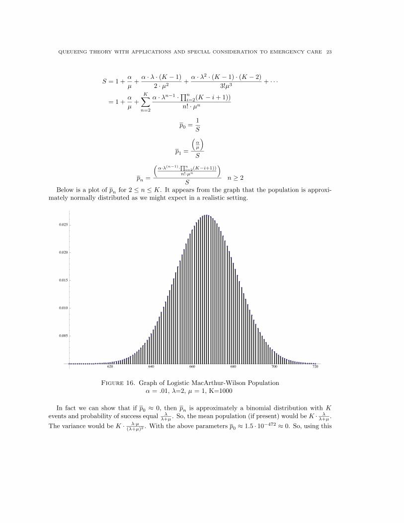
Below is a plot of pn for 2 ≤ n ≤ K. It appears from the graph that the population is approxi-mately normally distributed as we might expect in a realistic setting.

620 640 660 680 700 720

0.005

0.010

0.015

0.020

0.025

Figure 16. Graph of Logistic MacArthur-Wilson Populationα = .01, λ=2, µ = 1, K=1000

In fact we can show that if p0 ≈ 0, then pn is approximately a binomial distribution with Kevents and probability of success equal λ

λ+µ . So, the mean population (if present) would be K · λλ+µ .

The variance would be K · λ·µ(λ+µ)2 . With the above parameters p0 ≈ 1.5 · 10−472 ≈ 0. So, using this

24 JAMES KEESLING

binomial approximation just mentioned, we have a mean population of approximately 667 with astandard deviation of 14.9. This seems a good fit for the graph.

Even if p0 6≈ 0, we can still approximate the conditional probabilities pn1−p0

for n ≥ 1.

pn1− p0

≈(K

n

)·(

λ

λ+ µ

)n·(

µ

λ+ µ

)K−n13. Probability of Extinction

An island population has to contend with limited resources. This is due to the limiting sizeof the island. This is what produces the limited carrying capacity. Due to this limited carryingcapacity, the population will become extinct with probability one. However, we can study theprocess by imagining that there are other immigrations after the extinction. For a population withlarge resources available, there is little loss in assuming that the population could grow withoutbound. In this case there is a positive probability that the population will never become extinct.In this section we give an indication why this is the case.

Suppose that we have a population that could grow without bound. The states would then beS = {0, 1, 2, . . . }. Suppose that the individual birth and death rates are λ and µ, respectively.Then this system can be represented by the following diagram.

0←−µ 1

λ−→←−2·µ· · ·

(n−1)·λ−→←−n·µ

nn·λ−→←−

(n+1)·µn+ 1 · · ·

In this case there will be long-term probabilities associated with the system. However, the sumof the pn will not be one. Assume that λ > µ. Let us follow the system until either the populationbecomes extinct, that is, n = 0, or until the population reaches some prescribed level, say n = N .This system can be modeled as a discrete Markov chain with states S = {0, 1, 2, . . . , N} and withthe following transition probabilities. Assuming 0 < n < N , the probability of going from n ton+ 1 is

pn,n+1 =nλ

nλ+ n mu=

λ

λ+ µ.

The probability of going from n to n− 1 is similarly given by

pn,n−1 =µ

λ+ µ.

The states n = 0 and n = N are absorbing states in this analysis. From finite Markov chaintheory we can determine the probability of ending in state 0 or N starting in state n. Let us useun to denote the probability of ending in state 0 starting in state n. The 1 − un will denote theprobability of ending in state N starting in state n. These probabilities are given below.

un =

(µλ

)n1−

(µλ

)N1− un =

1−(µλ

)n1−

(µλ

)NWe have approached the problem this way so that we can use the theory of finite Markov chains

to see what the probabilities are for reaching either of these two absorbing states. However, in the


case we started with N =∞. Taking in the limit in the formulas above we get that the probabilityof a population at level n going extinct is given below.

un =(µλ

)nThe probability of never going extinct is given by the following.

1− un = 1−(µλ

)nSo, for a population not limited by resources and starting in state n, we get that the steady-state

probabilities are given by the following.

p0 =(µλ

)npn = 0 for n > 0

So, the sum of these steady-state probabilities is not one. It is also the case that if the populationdoes not become extinct, then for any N , the probability is one that the population at some timet will exceed N and never be N or less for all time greater than t.

14. Acuity Analysis for Emergency Care

In this section we analyze a simple queueing system that illustrates a serious problem encounteredin emergency care. The problem is that those patients who arrive and are assigned a high acuitylevel on arrival are given first priority in being treated. The lower acuity level patients have lowpriority and must wait until all of the high acuity patients have been treated before their treatmentbegins.

There are give acuity levels in emergency care. These are standardized by the Emergency SeverityIndex or ESI number. The details of the ESI classification system can be found at the followinglink maintained by the Agency for Healthcare Research and Quality.

Our mathematical model is a simplified version of this system. We assume just two levels ofacuity. The first level has priority. Even if a patient from the second level of acuity is beingtreated and a first level patient arrives, the treatment is interrupted and the first priority patientimmediately begins treatment. We assume that there is just one server to begin with. Later wewill develop a more refined model. The purpose of the model is to show how congestion can occurby the introduction of a priority treatment system.

The parameters for this system is the following α1 = α · p1, the arrival rate of high prioritypatients. We denote the arrival rate of the low priority patients by α2 = α · p2. We assume thatthese are independent Poisson systems. The service rate for a high priority patient is σ1. Theservice rate for a low priority patient is σ2. There are two lines, one for the priority one patientsand one for the priority two patients. The only time that priority two patients are treated is whenthere are no priority one patients in the system. We visualize the system in the following way.

The patients in the first queue can be treated as an M/M/1/FIFO system. To those patientsand the facility, the other patients are virtually invisible. It is when only the system consisting ofthe first priority patients is in state zero that the patients in the second level of priority can betreated.

We have already analyzed the M/M/1/FIFO system. With the parameters that we have forthat system we have the following results for the first priority patients.

http://www.ahrq.gov/research/esi/esi1.htm

26 JAMES KEESLING

α1

α 2

σ 1

σ 2

Figure 17. Priority Queue with Two Levels of Priority

pn =

(α1

σ1

)n·(

1− α1

σ1

)

n = E(n) =α1

σ1(1− α1

σ1

)From this information we can determine the average time that it takes from the instant that the

priority one system goes from empty to non-empty to when it returns to empty once again. Let uscall this time T . The Ergodic Theorem gives us the formula.

p0 =

(1− α1

σ1

)=

1α1

1α1

+ T

This gives us the following value for T .

T =1

σ1 − α1

We can now determine the average time for the priority patient to complete his/her treatment.Let us label this time τ .

τ =σ2

σ2 + α1

( ∞∑n=0

(n+ 1) · 1

σ2 + α1

(α1

σ2 + α1

)n+ T

∞∑n=1

n ·(

α1

σ2 + α1

)n)This simplifies to the following.

(11) τ =σ1

(σ1 − α1) · σ2We are now in a position to at least give the average times that patients will spend in the system

given the number of patients already present. The priority one patients will spend an average of(n+ 1) · 1

σ1time in the system. From the above formula for n for the priority one patients, we get

the following average time.

(n+ 1) · 1

σ1=

1

σ1 − α1

Now suppose that a patient comes into the system with n1 priority one patients in line and n2priority two patients in line. Let us call the time to complete service for an arriving priority onepatient T1(n1, n2) and the time to complete service for the second priority patient T2(n1, n2). Ifthe patient is priority one, then the time waiting is the following.


T1(n1, n2) = (n1 + 1) · 1

σ1The n2 priority two patients play no role in how long it will take this patient to finish treatment.How long will it take for a priority two patient to finish treatment coming to a system with n1

priority one patients and n2 priority two patients? First, the system must be cleared of all priorityone patients. This will include the n1 patients already there plus any others that might arriveduring the time that these n1 are being treated. The time for the priority one system to get to zerofrom n1 is just n1

σ1. On the other hand, once the priority one system is in state zero, then the time

for the n2 priority two patients to complete treatment is just n2 · τ where τ was computed above.Thus, the total time for the priority two patient to complete treatment will be the following.

T2(n1, n2) =n1σ1

+ (n2 + 1) · τ =n1σ1

+(n2 + 1) · σ1

(σ1 − α1) · σ2It would be good to know the average waiting time for patients who are assigned priority two.

To do this we would need to compute the long-term probabilities p(n1,n2) of being in each state

(n1, n2). We do not have simple formulas for these at the present time. However, we still havediscovered formulas for the total time waiting and being served.

15. Acuity Analysis of Emergency Care - Continued

Consider the two level priority queue that was discussed in the last section. Assume that theparameters α1, σ1, α2 and σ2 represent that arrival rate and service rate for the priority one andtwo level patients, respectively. We now derive the service time τ in (11) in a simpler way. Theservice time, τ , for a priority two patient can be thought of as a sum of the basic service time, 1

σ2,

together with an interruption time, S, due to the arrival of priority one patients..

τ =1

σ2+ S

The interruption time can be seen to be given by the following equation.

S = α1 ·(

1

σ2+ S

)· 1

σ1We can solve for S and substitute into the equation for τ to get the formula that we got by a

more complicated process in the previous section.

τ =σ1

(σ1 − α1) · σ2However, let us write τ in a different way.

(12) τ =1σ2(

1−(α1

σ1

))In the form of (12) we can see that τ is the average service time without interruption 1

σ2divided

by the probability that the priority one system is in the zero state 1 − α1

σ1. This tells us precisely

how the service time is being increased by the interruptions of priority one patients and how toadjust.

28 JAMES KEESLING

Consider an example. Suppose that the priority one system has α1 = 9 and σ1 = 10. Thenthe traffic intensity is α1

σ1= 9

10 . In this case, we get a dramatic change in the service time for thepriority two patients.

τ = 10 · 1

σ2The actual service time is ten times what it would normally be without interruptions. This is

true for every priority two patient in front of this patient. If there are five patients in front of thispatient, then the total time in the system will be sixty times the time it would normally take forthat patient finally complete treatment. This makes more clear how assigning priority can makethe system extremely congested.

Note also that if we had α1 = 9, α2 = 12 , σ1 = 10, and σ2 = 10, then if there were no distinctions

between priority one and two patients, we would have a M/M/1/FIFO queueing system withα = 9.5 and σ = 10. The system would be in equilibrium even though there might be longer lines

than would be desirable. The actual average n =9.510

1− 9.510

= 19. Let is compare this with the two

priority system. The service rate for priority two patients must be adjusted. The new rate is notσ2 but

σ2 =1

τ= σ2 ·

(1− α1

σ1

)In the case we have been considering, σ2 = σ2

10 . The system is also at equilibrium since α2 = 12 <

σ2 = 1. However, the average time being served for a priority two patient is ten times the servicetime. So, if there are three priority patients in line before that patient arrived, then the total timebeing served would be forty times the service time.

We will have a clearer picture when we can compute the steady-state probabilities. However, themodel is giving a sense of the congestion and inconvenience that arises through the priority system.

Of course, in emergency care, there are compelling reasons that priority one patients are treatedfirst. They are facing life-threatening circumstances. However, the overcrowding and gridlock thatsome emergency rooms are now facing make it clear that something must be done to bring relief tothose enduring the long waiting times getting treatment. The average median time for emergencycare from registration to discharge is more than four hours. This is several times the median timethat the care itself would require.

16. Higher Levels of Acuity

Now consider the case that we have several levels of acuity: priority 1, priority 2, . . . , priorityn. Each level takes priority over those levels below in the same fashion as the case above. Below isa diagram that illustrates this situation.

In this case we can also derive the modified service time for those in priority n.

τn =1σn

1−∑n−1i=1

αiσi

Of course, for each level of priority we also have a modified service time, namely:

τm =1σm

1−∑m−1i=1

αiσi

.


Figure 18. Priority Queue with Multiple Levels of Priority

For an equilibrium to exist, it is clear that σi > αi must hold for all for all 1 ≤ n. We can nowsee also that

n−1∑i=1

αiσi

< 1

must hold.There is also modified rate of service for each i, namely:

σi = σi ·

1−i−1∑j=1

αjσj

.

For each of these modified rates of service, σi > αi must hold for an equilibrium to exist. So,there are more criteria that must hold for equilibrium than first meets the eye.

Note that there is an easy fix for this situation. Instead of one server with all the interruptionscaused by multiple priorities, simply have a separate server for each priority or at least for thosewith the highest α

σ ratio. For example, consider a two priority system with α1

σ1= α2

σ2= 1

2 . Then the

priority system is not stable since 1 − α1

σ1− α2

σ2= 0. However, separating the two priority clients

and treating them with separate facilities would yield two M/M/1/FIFO queues each of which hasασ = 1

2 < 1. So, both are stable and will have reasonable waiting times. The cost is the additionof a server. However, the server for priority two patients would likely be less expensive than theserver for priority one patients.

In real life many factors must be taken into account. However, the mathematical models consid-ered in the last three sections give insights that are not likely to be seen otherwise. If it is necessaryto take other factors into account, more sophisticated models can be constructed and simulationsperformed to see the effect of those factors.

In the next section we will develop a method for determining the steady-state probabilities forpriority queues.

17. Simulation of Priority Queues with Preemption

Here we discuss a realistic model of Emergency Care developed by our research group. It is asimulation program written in R. The program was produced by Joshua Hurwitz on collaboration

30 JAMES KEESLING

with Jo Ann Lee. It was a project in a class taught by Professor Scott McKinley who was alsoinvolved in the project. The program simulates the number of patients in each of the five ESI levelsof priority through a period of several days. For the parameters that fit the arrival rates and staffingat the Shands ED, we get a good fit. The simulation model linked below allows one to adjust theparameters and observe the results of the simulation.

The program assumes that each priority class preempts those of lower priority classes. Thepreemption includes interruption of treatment of a lower priority patient so that treatment timesare longer than would be anticipated. Experimenting with the program shows how easily congestionarises. Examination of the graphs produced by the program shows that one should be able toanticipate the congestion and perhaps take measures to bring on additional personnel to avoid theextreme waiting times. We hope that these simulations will allow hospital management to recognizecriteria that indicate when congestion is likely to occur. If we can recognize when congestion islikely to occur, then staffing could be arranged to prevent it.

The paper describing the simulation program was published as, ”A comprehensive simulationplatform to quantify and manage site-specific emergency department crowding” Biomed CentralMedical Informatics and Decision Making, http://www.biomedcentral.com/1472-6947/14/50

(online publication: Joshua Hurwitz, Jo Ann Lee, Kenneth Lopiano, Scott McKinley, JamesKeesling, Joseph Tyndall). There is a software website demonstrating the simulation platformhttp://spark.rstudio.com/klopiano/EDsimulation/.

References

[1] Francois Baccelli and Pierre Bremaud. Elements of Queueing Theory. Springer-Verlag, Berlin, second edition,2010.

[2] Lothar Breuer and Dieter Baum. An Introduction to Queueing Theory and Matrix-Analytic Methods. Springer,

Dordrecht, Netherlands, 2005.[3] Jody Crane and Chuck Noon. The Definitive Guide to Emergency Department Operational Improvement. CRC,

Boca Raton, Florida, 2011.

[4] Giovanni Giambene. Queueing Theory and Telecommunications. Springer, New York, 2005.[5] Donald Gross, John F. Shortle, James M. Thompson, and Carl M. Harris. Fundamentals of Queueing Theory.

John Wiley, Hoboken, New Jersey, 2008.

[6] Shaler Sticham Jr. Optimal Design of Queueing Sytems. CRC, Boca Raton, Florida, 2009.[7] Leonard Kleinrock. Queueing Systems. John Wiley, Hoboken, New Jersey, 1975.

[8] Robert H. MacArthur and Edward O. Wilson. The Theory of Island Biogeography. Princeton University Press,Princeton, 1967.

[9] William Stewart. Probability, Markov Chains, Queues, and Simulation: the Mathematical Basis of Performance

Modeling. Princeton Press, Princeton, New Jersey, 2009.

http://www.biomedcentral.com/1472-6947/14/50

http://spark.rstudio.com/klopiano/EDsimulation/

queueing theory with applications and … theory with applications and special consideration to...

Documents