Queue-based Multi-processing Lisp

Richard P. GabrielJohn McCarthy

Stanford University

1. Introduction

As the need for high-speed computers increases, the need for multi-processors will bebecome more apparent. One of the major stumbling blocks to the development of usefulmulti-processors has been the lack of a good multi-processing language—one which is bothpowerful and understandable to programmers.

Among the most compute-intensive programs are artificial intelligence (AI) programs,and researchers hope that the potential degree of parallelism in AI programs is higher thanin many other applications. In this paper we propose multi-processing extensions to Lisp.Unlike other proposed multi-processing Lisps, this one provides only a few very powerfuland intuitive primitives rather than a number of parallel variants of familiar constructs.

Support for this research was provided by the Defense Advanced Research Projects Agency under

Contract DARPA/N00039-82-C-0250

1

§ 2 Design Goals

2. Design Goals

1. Because Lisp manipulates pointers, this Lisp dialect will run in a shared-memory architec-ture;

2. Because any real multi-processor will have only a finite number of CPU’s, and becausethe cost of maintaining a process along with its communications channels will not be zero,there must be a means to limit the degree of multi-processing at runtime;

3. Only minimal extensions to Lisp should be made to help programmers use the new con-structs;

4. Ordinary Lisp constructs should take on new meanings in the multi-processing setting,where appropriate, rather than proliferating new constructs.

5. The constructs should all work in a uni-processing setting (for example, it should bepossible to set the degree of multi-processing to 1 as outlined in point 2); and

3. This Paper

This paper presents the added and re-interpreted Lisp constructs, and examples ofhow to use them are shown. A simulator for the language has been written and usedto obtain performance estimates on sample problems. This simulator and some of theproblems are be briefly presented.

4. QLET

The obvious choice for a multi-processing primitive for Lisp is one which evaluatesarguments to a lambda-form in parallel. QLET serves this purpose. Its form is:

(QLET pred ((x1arg1)...

(xn argn)). body)

Pred is a predicate that is evaluated before any other action regarding this form istaken; it is assumed to evaluate to one of: (), EAGER, or something else.

If pred evaluates to (), then the QLET acts exactly as a LET. That is, the argumentsarg1 . . . argn are evaluated as usual and their values bound to x1 . . . xn, respectively.

2

§ 4 QLET

If pred evaluates to non-(), then the QLET will cause some multi-processing to hap-pen. Assume pred returns something other than () or EAGER. Then processes arespawned, one for each argi. The process evaluating the QLET goes into a wait state:When all of the values arg1 . . . argn are available, their values are bound to x1 . . . xn, re-spectively, and each form in the list of forms, body, is evaluated.

Assume pred returns EAGER. Then QLET acts exactly as above, except that theprocess evaluating the QLET does not wait: It proceeds to evaluate the forms in body.But if in evaluating the forms in body the value of one of the arguments is required, argi,the process evaluating the QLET waits. If that value has been supplied already, it issimply used.

To implement EAGER binding, the value of the EAGER variables could be set toan ‘empty’ value, which could either be an empty memory location, like that supportedby the Denelcor HEP [Smith 1978], or a Lisp object with a tag field indicating an emptyor pending object. At worst, every use of a value would have to check for a full pointer.

We will refer to this style of parallelism as QLET application.

4.1 Queue-based

The Lisp is described as ‘queue-based’ because the model of computation is thatwhenever a process is spawned, it is placed on a global queue of processes. A schedulerthen assigns that process to some processor. Each processor is assumed to be able to runany number of processes, much as a timesharing system does, so that regardless of thenumber of processes spawned, progress will be made. We will call a process running on aprocessor a job.

The ideal situation is that the number of processes active at any one time will beroughly equal to the number of physical processors available.1

The idea behind pred, then, is that at runtime it is desirable to control the numberof processes spawned. Simulations show a marked dropoff in total performance as the

1 Strictly speaking this isn’t true. Simulations show that the ideal situation depends on the length

of time it takes to create a process and the amount of waiting the average process needs to do. If the

creation time is short, but realistic, and if there is a lot of waiting for values, then it is better to use some

of the waiting time creating active processes, so that no processor will be idle. The ideal situation has no

physical processor idle.

3

§ 4 QLET

number of processes running on each processor increases, assuming that process creationtime is non-zero.

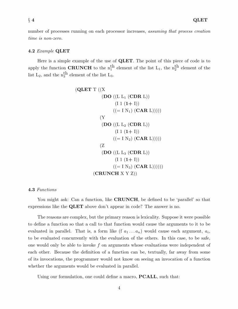
4.2 Example QLET

Here is a simple example of the use of QLET. The point of this piece of code is toapply the function CRUNCH to the nth

1 element of the list L1, the nth2 element of the

list L2, and the nth3 element of the list L3.

(QLET T ((X(DO ((L L1 (CDR L))

(I 1 (1+ I))((= I N1) (CAR L)))))

(Y(DO ((L L2 (CDR L))

(I 1 (1+ I))((= I N2) (CAR L)))))

(Z(DO ((L L3 (CDR L))

(I 1 (1+ I))((= I N3) (CAR L))))))

(CRUNCH X Y Z))

4.3 Functions

You might ask: Can a function, like CRUNCH, be defined to be ‘parallel’ so thatexpressions like the QLET above don’t appear in code? The answer is no.

The reasons are complex, but the primary reason is lexicality. Suppose it were possibleto define a function so that a call to that function would cause the arguments to it to beevaluated in parallel. That is, a form like (f a1 . . . an) would cause each argument, ai,to be evaluated concurrently with the evaluation of the others. In this case, to be safe,one would only be able to invoke f on arguments whose evaluations were independent ofeach other. Because the definition of a function can be, textually, far away from someof its invocations, the programmer would not know on seeing an invocation of a functionwhether the arguments would be evaluated in parallel.

Using our formulation, one could define a macro, PCALL, such that:

4

§ 4 QLET

(PCALL f a1 . . . an)

would accomplish parallel argument evaluation. Of course, this is just a macro for a QLET

application.

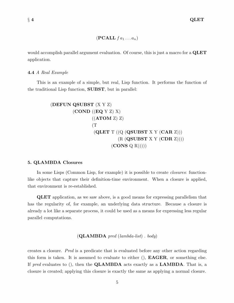
4.4 A Real Example

This is an example of a simple, but real, Lisp function. It performs the function ofthe traditional Lisp function, SUBST, but in parallel:

(DEFUN QSUBST (X Y Z)(COND ((EQ Y Z) X)

((ATOM Z) Z)(T(QLET T ((Q (QSUBST X Y (CAR Z)))

(R (QSUBST X Y (CDR Z))))(CONS Q R)))))

5. QLAMBDA Closures

In some Lisps (Common Lisp, for example) it is possible to create closures: function-like objects that capture their definition-time environment. When a closure is applied,that environment is re-established.

QLET application, as we saw above, is a good means for expressing parallelism thathas the regularity of, for example, an underlying data structure. Because a closure isalready a lot like a separate process, it could be used as a means for expressing less regularparallel computations.

(QLAMBDA pred (lambda-list) . body)

creates a closure. Pred is a predicate that is evaluated before any other action regardingthis form is taken. It is assumed to evaluate to either (), EAGER, or something else.If pred evaluates to (), then the QLAMBDA acts exactly as a LAMBDA. That is, aclosure is created; applying this closure is exactly the same as applying a normal closure.

5

§ 5 QLAMBDA Closures

If pred evaluates to something other than EAGER, the QLAMBDA creates a closurethat, when applied, is run as a separate process. Creating the closure by evaluating theQLAMBDA expression is called spawning; the process that evaluates the QLAMBDA

is called the spawning process; and the process that is created by the QLAMBDA is calledthe spawned process. When a closure running as a separate process is applied, the separateprocess is started, the arguments are evaluated by the spawning process, and a messageis sent to the spawned process containing the evaluated arguments and a return address.The spawned process does the appropriate lambda-binding, evaluates its body, and finallyreturns the results to the spawning process. We call a closure that will run or is runningin its own process a process closure. In short, the expression (QLAMBDA non-() . . .)returns a process closure as its value.

If pred evaluates to EAGER, then a closure is created which is immediately spawned.It lambda-binds empty binding cells as described earlier, and evaluation of its body startsimmediately. When an argument is needed, the process either has had it supplied or itblocks. Similarly, if the process completes before the return address has been supplied, theprocess blocks.

This curious method of evaluation will be used surprisingly to write a parallel Y

function!

5.1 Value-Requiring Situations

Suppose there are no further rules for the timing of evaluations than those given, alongwith their obvious implications; have we defined a useful set of primitives?

No. Consider the situation:

(PROGN (F X) (G Y))

If F happens to be bound to a process closure, then the process evaluating the PROGN

will spawn off the process to evaluate (F X), wait for the result, and then move on toevaluate (G Y), throwing away the value F returned. If this is the case, it is plain thatthere is not much of a reason to have process closures.

Therefore we make the following behavioral requirement: If a process closure is calledin a value-requiring context, the calling process waits; and if a process closure is called in

6

§ 5 QLAMBDA Closures

a value-ignoring situation, the caller does not wait for the result, and the callee is given avoid return address.

For example, given the following code:

(LET ((F (QLAMBDA T (Y)(PRINT (∗ Y Y)))))(F 7)(PRINT (∗ 6 6)))

there is no a priori way to know whether you will see 49 printed before or after 36.2

To increase the readability of code we introduce two forms, which could be defined asmacros, to guarantee a form will appear in a value-requiring or in a value-ignoring position.

(WAIT form)

will evaluate form and wait for the result;

(NO-WAIT form)

will evaluate form and not wait for the result.

For example,

(PROGN

(WAIT form1)form2)

will wait for form1 to complete.

2 We can assume that there is a single print routine that guarantees that when something is printed,

no other print request interferes with it. Thus, we will not see 43 and then 96 printed in this example.

7

§ 5 QLAMBDA Closures

5.2 Applying a Process Closure

Process closures can be passed as arguments and returned as values. Therefore, aprocess closure can be in the middle of evaluating its body given a set of arguments whenit is applied by another process. Similarly, a process can apply a process closure in a value-ignoring position and then immediately apply the same process closure with a different setof arguments.

Each process closure has a queue for arguments and return addresses. When a processclosure is applied, the new set of arguments and the return address is placed on this queue.The body of the process closure is evaluated to completion before the set of arguments atthe head of the queue is processed.

We will call this property integrity, because a process closure is not copied or disruptedfrom evaluating its body with a set of arguments: Multiple applications of the same processclosure will not create multiple copies of it.

6. CATCH and QCATCH

So far we have discussed methods for spawning processes and communicating results.Are there any ways to kill processes? Yes, there is one basic method, and it is based onan intuitively similar, already-existing mechanism in many Lisps.

CATCH and THROW are a way to do non-local, dynamic exits within Lisp. Theidea is that if a computation is surrounded by a CATCH, then a THROW will forcereturn from that CATCH with a specified value, terminating any intermediate computa-tions.

(CATCH tag form)

will evaluate form. If form returns with a value, the value of the CATCH expression isthe value of the form. If the evaluation of form causes the form

(THROW tag value)

to be evaluated, then CATCH is exited immediately with the value value. THROW

causes all special bindings done between the CATCH and the THROW to revert. If

8

§ 6 CATCH and QCATCH

there are several CATCH’s, the THROW returns from the CATCH dynamically closestwith a tag EQ to the THROW tag.

6.1 CATCH

In a multi-processing setting, when a CATCH returns a value, all processes that werespawned as part of the evaluation of the CATCH are killed at that time.

Consider:

(CATCH ’QUIT(QLET T ((X

(DO ((L L1 (CDR L)))((NULL L) ’NEITHER)(COND ((P (CAR L))

(THROW ’QUIT L1)))))(Y(DO ((L L2 (CDR L)))

((NULL L) ’NEITHER)(COND ((P (CAR L))(THROW ’QUIT L2))))))

X))

This piece of code will scan down L1 and L2 looking for an element that satisfies P. Whensuch an element is found, the list that contains that element is returned, and the otherprocess is killed, because the THROW causes the CATCH to exit with a value. If bothlists terminate without such an element being found, the atom NEITHER is returned.

Note that if L1 and L2 are both circular lists, but one of them is guaranteed to containan element satisfying P, the entire process terminates.

If a process closure was spawned beneath a CATCH and if that CATCH returnswhile that process closure is running, that process closure will be killed when the CATCH

returns.

6.2 QCATCH

(QCATCH tag form)

9

§ 6 CATCH and QCATCH

QCATCH is similar to CATCH, but if the form returns with a value (no THROW

occurs) and there are other processes still active, QCATCH will wait until they all finish.The value of the QCATCH is the value of form. For there to be any processes activewhen form returns, each one had to have been applied in a value-ignoring setting, andtherefore all of the values of the outstanding processes will be duly ignored.

If a THROW causes the QCATCH to exit with a value, the QCATCH kills allprocesses spawned beneath it.

We will define another macro to simplify code. Suppose we want to spawn the evalu-ation of some form as a separate process. Here is one way to do that:

((LAMBDA (F)(F) T)

(QLAMBDA T () form))

A second way is:

(FUNCALL (QLAMBDA T () form))

We will chose the latter as the definition of:

(SPAWN form)

Notice that SPAWN combines spawning and application.

Here are a pair of functions which work together to define a parallel EQUAL functionon binary trees:

(DEFUN EQUAL (X Y)(QCATCH ’EQUAL

(EQUAL-1 X Y)))

EQUAL uses an auxiliary function, EQUAL-1:

10

§ 6 CATCH and QCATCH

(DEFUN EQUAL-1 (X Y)(COND ((EQ X Y))

((OR (ATOM X)(ATOM Y))

(THROW ’EQUAL ()))(T(SPAWN (EQUAL-1 (CAR X)(CAR Y)))(SPAWN (EQUAL-1 (CDR X)(CDR Y)))T)))

The idea is to spawn off processes that examine parts of the trees independently. Ifthe trees are not equal, a THROW will return a () and kill the computation. If the treesare equal, no THROW will ever occur. In this case, the main process will return T to theQCATCH in EQUAL. This QCATCH will then wait until all of the other processesdie off; finally it will return this T.

6.3 THROW

THROW will throw a value to the CATCH above it, and processes will be killedwhere applicable. The question is, when a THROW is seen, exactly which CATCH isthrown to and exactly which processes will be killed?

The processes that will be killed are precisely those processes spawned beneath theCATCH that receives the THROW and those spawned by processes spawned beneaththose, and so on.

The question boils down to which CATCH is thrown to. To determine that CATCH,find the process in which the THROW is evaluated and look up the process-creation chainto find the first matching tag.

If you see a code fragment like:

(QLAMBDA T () (THROW tag value))

the THROW is evaluated within the QLAMBDA process closure, so look at the processin which the QLAMBDA is created to start searching for the proper CATCH. Thus,if you apply a process closure with a THROW in it, the THROW will be to the first

11

§ 6 CATCH and QCATCH

CATCH with a matching tag in the process chain that the QLAMBDA was created in,not in the current process chain.

Thus we say that THROW throws dynamically by creation.

7. UNWIND-PROTECT

When THROW is used to terminate a computation, there may be other actions thatneed to be performed before the context is destroyed. For instance, suppose that some fileshave been opened and their streams lambda-bound. If the bindings are lost, the files willremain open until the next garbage collection. There must be a way to gracefully closethese files when a THROW occurs. The construct to do that is UNWIND-PROTECT.

(UNWIND-PROTECT form cleanup)

will evaluate form. When form returns, cleanup is evaluated. If form causes a THROW

to be evaluated, cleanup will be performed anyway. Here is a typical use:

(LET ((F (OPEN “FOO.BAR”)))(UNWIND-PROTECT (READ-SOME-STUFF) (CLOSE F)))

In a multi-processing setting, when a cleanup form needs to be evaluated because aTHROW occurred, the process that contains the UNWIND-PROTECT is retained toevaluate all of the cleanup forms for that process before it is killed. The process is placedin an un-killable state, and if a further THROW occurs, it has no effect until the currentcleanup forms have been completed,.

Thus, if control ever enters an UNWIND-PROTECT, it is guaranteed that thecleanup form will be evaluated. Dynamically nested UNWIND-PROTECT’s will havetheir cleanup forms evaluated from the inside-out, even if a THROW has occurred.

To be more explicit, recall that the CATCH that receives the value thrown by aTHROW performs the kill operations. The UNWIND-PROTECT cleanup forms areevaluated in un-killable states by the appropriate CATCH before any kill operations areperformed. This means that the process structure below that CATCH is left in tact untilthe UNWIND-PROTECT cleanup forms have completed.

12

§ 7 UNWIND-PROTECT

7.1 Other Primitives

One pair of primitives is useful for controlling the operation of the processes as theyare running; they are SUSPEND-PROCESS and RESUME-PROCESS. The formertakes a process closure and puts it in a wait state. This state cannot be interrupted,except by a RESUME-PROCESS, which will resume this process. This is useful ifsome controlling process wishes to pause some processes in order to favor some processmore likely to succeed than these.

A use for SUSPEND-PROCESS is to implement a general locking mechanism,which will be described later.

7.2 An Unacceptable Alternative

There is another approach that could have been taken to the semantics of:

(QLAMBDA pred (lambda-list) . body)

Namely, we could have stated that the arguments to a process closure could trickle in,some from one source and some from another. Because a process closure could then needto wait for arguments from several sources, we could use this behavior as a means to achievethe effects of SUSPEND-PROCESS. That is, we could apply a process closure whichrequires one argument to no arguments; the process closure would then need to wait foran argument to be supplied. Because we would not supply that argument until we wantedthe process to continue, supplying the argument would achieve RESUME-PROCESS.

This would be quite elegant, but for the fact that process closures would then beable to get arguments from anywhere chaotically. We would have to abandon the abilityto know the order of variable-value pairing in the lambda-binding that occurs in processclosures. For instance, if we had a process closure that took two arguments, one a numberand the other a list, and if one argument were to be supplied by one process and thesecond by another, there would be no way to cause one argument to arrive at the processclosure before the other, and hence one would not be sure that the number paired withthe variable that was intended to have a numeric value.

One could use keyword arguments [Steele 1984] in this case, but that would not solveall the problems with this scheme. How could &REST arguments be handled? Therewould be no way to know when all of the arguments to the process closure had been

13

§ 7 UNWIND-PROTECT

supplied. Suppose that a process wanted to send 5 values to a process closure that neededexactly 5 arguments; if some other process had sent 2 to that process closure already, howcould one require that the first 3 of the 5 sent would not be bundled with the 2 alreadysent to supply the process closure with random arguments?

In short, this alternative is unacceptable.

8. The Rest of the Paper

This completes the definition of the extensions to Lisp. Although these primitives forma complete set—any concurrent algorithm can be programmed with only these primitivesalong with the underlying Lisp—a real implementation of these extensions would supplyfurther convenient functions, such as an efficient locking mechanism.

The remainder of this paper will describe some of the tricky things that can be done inthis language, and it will present some performance studies done with a simple simulator.

9. Resource Management

We’ve mentioned that we assume a shared-memory Lisp, which implies that manyprocesses can be accessing and updating a single data structure at the same time. Inthis section we show how to protect these data structures with critical sections to allowconsistent updates and accesses.

The key is closures. We spawn a process closure which is to be used as the solemanager of a given resource, and we conduct all transactions through that closure. Weillustrate the method with an example.

Suppose we have an application where we will need to know for very many n whether∃ i s.t. n = Fib(i), where Fib is the Fibonacci function. We will call this predicate Fib-p.Suppose further that we want to keep a global table of all of the Fibonacci argument/valuepairs known, so that Fib-p will be a table lookup whenever possible. We can use a variable,∗V∗, which has a pair—a cons cell—as its value with the CAR being i and the CDR

being n, and n = Fib(i), such that this is the largest i in the table. We imagine filling upthis table as needed, using it as a cache, but the variable ∗V∗ is used in a quick test todecide whether to use the table rather than Fibonacci function to decide Fib-p.

We will ignore the details of the table manipulation and discuss only the variable ∗V∗.When a process wants to find out the highest Fibonacci number in the table, it simply will

14

§ 9 Resource Management

do (CDR ∗V∗). If a process wants to find out the pair (i . Fib(i)), it had better do thisindivisibly because some other processes might updating ∗V∗ concurrently.

We assume that we do not want to CONS another pair to update ∗V∗—we willdestructively update the pair. Thus, we do not want to say:

. . .

(SETQ ∗V∗ (CONS arg val)). . .

Here is some code to set up the ∗V∗ handler:

(SETQ ∗V-HANDLER∗ (QLAMBDA T (CODE) (CODE *V*)))

The idea is to pass this process closure a second closure which will perform the desiredoperations on its lone argument; the ∗V∗ handler passes ∗V∗ to the supplied closure.

Here is a code fragment to set up two variables, I and J, which will receive the valuesof the components of ∗V∗, along with the code to get those values:

(LET ((I ())(J ()))(∗V-HANDLER∗ (LAMBDA (V)

(SETQ I (CAR V))(SETQ J (CDR V))))

. . .)

Because the process closure will evaluate its body without creating any other copiesof itself, and because all updates to ∗V∗ will go through ∗V-HANDLER∗, I and J willbe such that J = Fib(I).

The code to update the value of ∗V∗ would be:

. . .

(∗V-HANDLER∗ (LAMBDA (V)(SETF (CAR V) arg)(SETF (CDR V) val)))

. . .

15

§ 9 Resource Management

If the process updating ∗V∗ does not need to wait for the update, this call can be putin a value-ignoring position.

9.1 Fine Points

If the process closure that controls a resource is created outside of any CATCH orQCATCH that might be used to terminate subordinate process closures, then once theprocess closure has been invoked, it will be completed. If this process closure is busy whenit is invoked by some process, then even if the invoking process is killed, the invocationwill proceed. Thus requests on a resource controlled by this process closure are alwayscompleted. Another way to guarantee that a request happens is to put it inside of anUNWIND-PROTECT.

10. Locks

When we discussed SUSPEND-PROCESS and RESUME-PROCESS we men-tioned that a general locking mechanism could be implemented using SUSPEND-PRO-

CESS. Here is the code for this example:

(DEFMACRO GET-LOCK ()’(CATCH ’FOO

(PROGN

(LOCK(QLAMBDA T (RES)(THROW ’FOO RES)))

(SUSPEND-PROCESS))))

When SUSPEND-PROCESS is called with no arguments, it puts the currently runningjob (itself) into a wait state.

1 (LET ((LOCK2 (QLAMBDA T (RETURNER)3 (CATCH LOCKTAG4 (LET ((RES (QLAMBDA T () (THROW ’LOCKTAG T))))5 (RETURNER RES)6 (SUSPEND-PROCESS))))))

16

§ 10 Locks

7 (QLET T ((X8 (LET ((OWNED-LOCK (GET-LOCK)))9 (DO ((I 10 (1− I)))

10 ((= I 0)11 (OWNED-LOCK) 7))))12 (Y13 (LET ((OWNED-LOCK (GET-LOCK)))14 (DO ((I 10 (1− I)))15 ((= I 0)16 (OWNED-LOCK) 8))))))17 (LIST X Y))

The idea is to evaluate a GET-LOCK form, which in this case is a macro, that willreturn when the lock is available; at that point, the process that called the GET-LOCKform will have control of the lock and, hence, the resource in question. GET-LOCK returnsa function that is invoked to release the lock.

Lines 7–17 are the test of the locking mechanism: The QLET on line 7 spawns twoprocesses; the first is the LET on lines 8–11; the second is the LET on lines 13–16. Eachprocess will attempt to grab the lock, and when a process has that lock, it will count downfrom 10, release the lock, and return a number—either 7 or 8. The two numbers are putinto a list that is the return value for the test program.

As we mentioned earlier, when a process closure is evaluating its body given a set ofarguments, it cannot be disrupted—no other call to that process closure can occur untilthe previous calls are complete. To implement a lock, then, we must produce a processclosure that will return an unlocking function, but which will not actually return!

GET-LOCK sets up a CATCH and calls the LOCK function with a process closurethat will return from this CATCH. The value that the process closure throws will be thefunction we use to return the lock. We call LOCK in a value-ignoring position so that whenthe lock is finally released, LOCK will not try to return a value to the process evaluatingthe GET-LOCK form. The SUSPEND-PROCESS application will cause the processevaluating the GET-LOCK form to wait for the THROW that will happen when LOCKsends back the unlocking function.

LOCK takes a function, the RETURNER function, that will return the unlocking

17

§ 10 Locks

function. LOCK binds RES to a process closure that throws to the CATCH on line 3.This process closure is the function that we will apply to return the lock. The RE-TURNER function is applied to RES, which throws RES to the catch frame with tagFOO. Because (RETURNER RES) appears in a value-ignoring position, this process clo-sure is applied with no intent to return a value. Evaluation in LOCK proceeds with thecall to SUSPEND-PROCESS.

The effect is that the process closure that will throw to LOCKTAG—and which willeventually cause LOCK to complete—is thrown back to the caller of GET-LOCK, butLOCK does not complete. No other call to LOCK will begin to execute until the THROW

to LOCKTAG occurs—that is, when the function, OWNED-LOCK, is applied.

Hence, exactly one process at a time will execute with this lock.

The key to understanding this code is to see that when a THROW occurs, it searchesup the process-creation chain that reflects dynamically scoped CATCH’s. Because wespawned the process closure in GET-LOCK beneath the CATCH there, the THROW

in the process closure bound to RETURNER will throw to that CATCH, ignoring theone in LOCK. Similarly, the THROW that RES performs was created underneath theCATCH in LOCK, and so the process closure that throws to LOCKTAG returns fromthe CATCH in LOCK.

10.1 Reality.

As mentioned earlier, a real implementation of this language would supply an efficientlocking mechanism. We have tried to keep the number of primitives down to see whatwould constitute a minimum language.

11. Killing Processes

We’ve seen that a process can commit suicide, but is there any way to kill anotherprocess? Yes; the idea is to force a process to commit suicide. Naturally, everything mustbe set up correctly.

We’ll show a simple example of this ‘bomb’ technique.

Here is the entire code for this example:

1 (DEFUN TEST ()2 (LET ((BOMBS ()))

18

§ 11 Killing Processes

3 (LET ((BOMB-HANDLER4 (QLAMBDA T (TYPE ID MESSAGE)5 (COND ((EQ TYPE ’BOMB)6 (PRINT ‘(BOMB FOR ,ID))7 (PUSH ‘(,ID . ,MESSAGE) BOMBS))8 ((EQ TYPE ’KILL)9 (PRINT ‘(KILL FOR ,ID))

10 (FUNCALL

11 (CDR (ASSQ ID BOMBS)))12 T)))))13 (QLET ’EAGER ((X14 (CATCH ’QUIT (TESTER BOMB-HANDLER ’A)))15 (Y16 (CATCH ’QUIT (TESTER BOMB-HANDLER ’B))))17 (SPAWN

18 (PROGN (DO ((I 10. (1− I)))19 ((= I 0)20 (PRINT ‘(KILLING A))21 (BOMB-HANDLER ’KILL ’A ()))22 (PRINT ‘(COUNTDOWN A ,I)))23 (DO ((I 10. (1− I)))24 ((= I 0)25 (PRINT ‘(KILLING B))26 (BOMB-HANDLER ’KILL ’B ()))27 (PRINT ‘(COUNTDOWN B ,I)))))28 (LIST X Y)))))

29 (DEFUN TESTER (BOMB-HANDLER LETTER)30 (BOMB-HANDLER ’BOMB LETTER31 (QLAMBDA T () (THROW ’QUIT LETTER)))32 (DO ()(()) (PRINT LETTER)))

First we set up a process closure which will collect bombs and explode them. Line 2defines the variable that will hold the bombs. A bomb is an ID and a piece of code.Lines 3–12 define the bomb handler. It is a piece of code that takes a message type, an

19

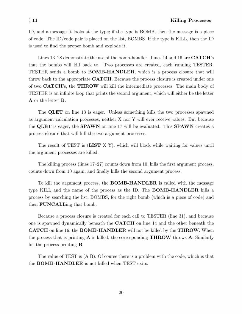
§ 11 Killing Processes

ID, and a message It looks at the type; if the type is BOMB, then the message is a pieceof code. The ID/code pair is placed on the list, BOMBS. If the type is KILL, then the IDis used to find the proper bomb and explode it.

Lines 13–28 demonstrate the use of the bomb-handler. Lines 14 and 16 are CATCH’sthat the bombs will kill back to. Two processes are created, each running TESTER.TESTER sends a bomb to BOMB-HANDLER, which is a process closure that willthrow back to the appropriate CATCH. Because the process closure is created under oneof two CATCH’s, the THROW will kill the intermediate processes. The main body ofTESTER is an infinite loop that prints the second argument, which will either be the letterA or the letter B.

The QLET on line 13 is eager. Unless something kills the two processes spawnedas argument calculation processes, neither X nor Y will ever receive values. But becausethe QLET is eager, the SPAWN on line 17 will be evaluated. This SPAWN creates aprocess closure that will kill the two argument processes.

The result of TEST is (LIST X Y), which will block while waiting for values untilthe argument processes are killed.

The killing process (lines 17–27) counts down from 10, kills the first argument process,counts down from 10 again, and finally kills the second argument process.

To kill the argument process, the BOMB-HANDLER is called with the messagetype KILL and the name of the process as the ID. The BOMB-HANDLER kills aprocess by searching the list, BOMBS, for the right bomb (which is a piece of code) andthen FUNCALLing that bomb.

Because a process closure is created for each call to TESTER (line 31), and becauseone is spawned dynamically beneath the CATCH on line 14 and the other beneath theCATCH on line 16, the BOMB-HANDLER will not be killed by the THROW. Whenthe process that is printing A is killed, the corresponding THROW throws A. Similarlyfor the process printing B.

The value of TEST is (A B). Of course there is a problem with the code, which is thatthe BOMB-HANDLER is not killed when TEST exits.

20

§ 12 Eager Process Closures

12. Eager Process Closures

We saw that EAGER is a useful value for the predicate in QLET applications, thatis, in constructions of this form:

(QLET pred ((x1arg1)...

(xn arg2)). body)

But it may not be certain what use it has in the context of a process closure.

When a process closure of the form:

(QLAMBDA ’EAGER (lambda-list) . body)

is spawned, it is immediately run. And if it needs arguments or a return address to besupplied, it waits.

Suppose we have a program with two distinct parts: The first part takes some time tocomplete and the second part takes some large fraction of that time to initialize, at whichpoint it requires the result of the first part. The easiest way to accomplish this is to starta eager process closure, which will immediately start running its initialization. When thefirst part is ready to hand its result to the process closure, it simply applies the processclosure.

Here is an example of this overlapping of a lengthy initialization with a lengthy com-putation of an argument:

(LET ((F (QLAMBDA ’EAGER (X)[Lengthy Initialization](OPERATE-ON X))))

(F [Lengthy computation of X]))

There are other ways to accomplish this effect in this language, but this is the mostflexible technique.

21

§ 12 Eager Process Closures

12.1 A Curious Example.

A curious example of this arises when the Y function is being defined in this language.

The Y function is the applicative version of the Y combinator, which can be used todefine LABELS (see Scheme [Steele 1978], [Sussman 1975]). We will briefly review theproblem that Y solves.

Suppose you write the code:

(LET ((CONS (LAMBDA (X Y) (CONS Y X)))) . . .),

will CONS refer to the CONS being defined or to the built-in CONS? The answer is thatit will refer to the built-in CONS, and this is not a non-terminating definition. It definesa constructor that builds lists in the CAR rather than the traditional CDR direction.

The idea is that the LAMBDA creates a closure that captures the environment atthe time of the closure creation, but this environment does not contain the binding forCONS because the process has not gotten that far yet—it is evaluating the form that willbe the value to place in the binding for CONS that it is about to make.

Suppose, though, that you want to define factorial in this style. You cannot write:

(LET ((FACT(LAMBDA (N)(COND ((ZEROP N) 1)

(T (∗ N (FACT (1− N)))))))). . .)

because the recursive call to FACT refers to some global definition, which presumablydoes not exist. Traditionally there is a LAMBDA-like form, called LABELS which getsaround this by creating a special environment and then re-stuffing the bindings appropri-ately, but there is a way to avoid introducing LABELS, at the expense of speed.

There is a function, called the Y function, that allows one to define a recursive functiongiven an abstraction of the ‘normal’ definition of the recursive function. Here is an exampleof the abstract version of FACT that we would need:

22

§ 12 Eager Process Closures

F = (LAMBDA (G)(LAMBDA (N)(COND ((ZEROP N) 1)

(T (∗ N (G (1- N)))))))

The key property of Y is: ∀f,Y(f) = f(Y(f)).

If we were to pass F the mathematical function fact, then F(fact) = fact in themathematical sense. That is, fact is a fixed point for F. If we define FACT to be Y(F),FACT is also a fixed point for F, using the property given above. Actually, Y producesthe least fixed point of F, but you can read about that in a textbook.

The definition of Y in Lisp is:

(DEFUN Y (F)(LET ((H (LAMBDA (G)

(F (LAMBDA (X)(FUNCALL (G G) X))))))

(LAMBDA (X) (FUNCALL (H H) X))))

We can trace through the operation of Y briefly. Y(F) returns a function that lookslike:

(LAMBDA (X) (FUNCALL (H H) X))

with H that looks like:

(LAMBDA (G)(F (LAMBDA (X)

(FUNCALL (G G) X))))

and F is bound to F above. What does (H H) return? Well, it is F applied to somefunction, so it returns the inner LAMBDA closure—(LAMBDA (N) . . .)—in F above,which will be applied to X: a good sign.

H takes a function—itself in this case—and binds it to the variable G. We can substi-tute H for G throughout to get F being applied to:

23

§ 12 Eager Process Closures

(LAMBDA (X) (FUNCALL (H H) X))

But F simply makes up a closure that binds the variable G to the above closure and returnsit. So if evaluation ever applies G to something, it simply applies the above closure to itsargument. G would be applied to something in the event that a recursive call was to bemade. H is still bound as before, and the F within the H closure is bound to the codefor F. Thus we end up in the same situation as we were at the outset (that is what theproperty ∀f,Y(f) = f(Y(f)) means!).

The machinations of this construction have the effect of providing another approxi-mation to the function fact as it is needed, by carefullly packaging up new closures thatwill present the code for F over and over as needed.

This is pretty expensive in time and space. It turns out that we can define QY asfollows:

(DEFUN QY (F)(LET ((H (LAMBDA (G)

(F (QLAMBDA ’EAGER (X)(FUNCALL (G G) X))))))

(QLAMBDA ’EAGER (X)(CATCH (NCONS ()) (FUNCALL (H H) X)))))

QY is just like Y, except that the major closures are eager process closures, andthere is a CATCH at the toplevel. The eager process closure at the toplevel will rununtil it blocks, which means until it needs the value of X. So (H H) will begin to beevaluated immediately. Likewise, subsequent applications of F will start off some pre-processing. Essentially, QY will start spawning off processes that will be pre-computingthe approximations spontaneously. They block when they need return addresses, but theyare ready to go when the main process, the one calculating factorial, gets around to them.

The CATCH stops the spawning process when we get to the end.

The performance of QY is between that of Y and LABELS, because QY pipelinesthe creation of the approximations.

24

§ 13 Performance

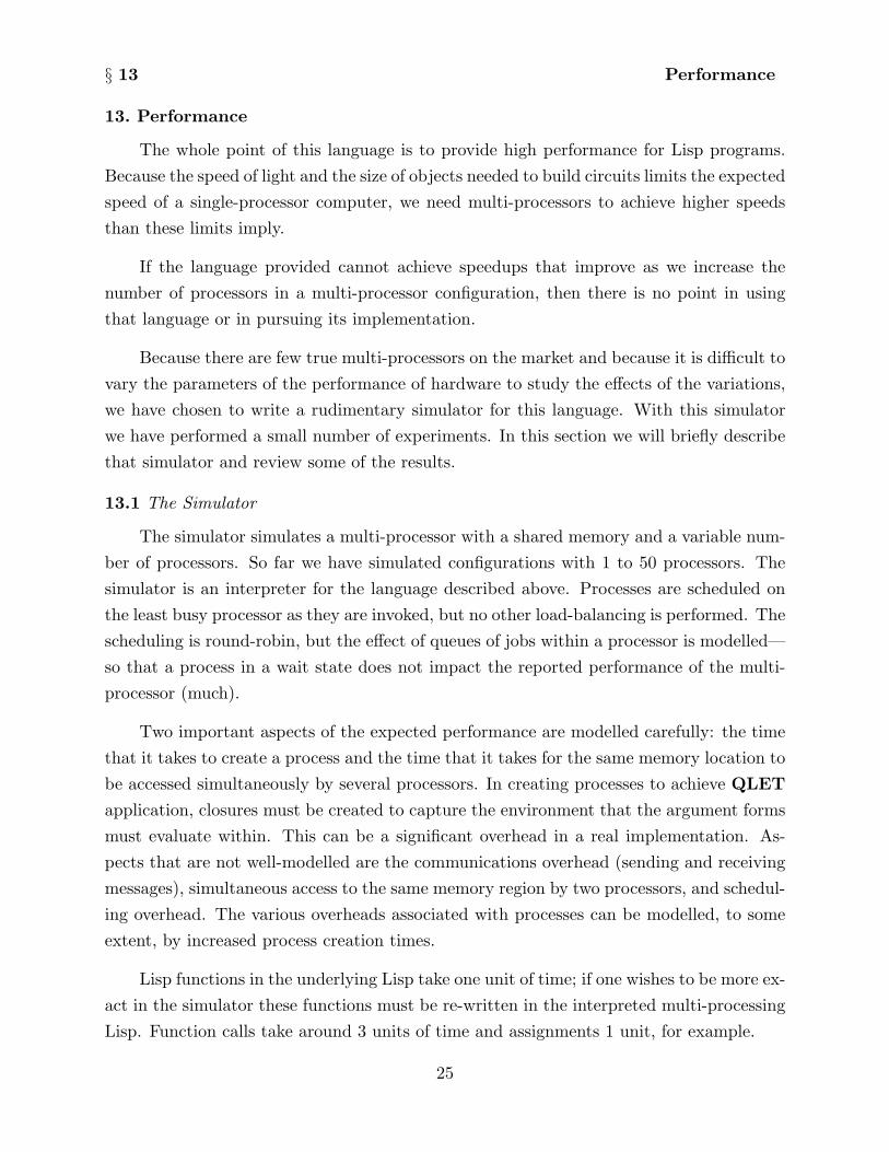
13. Performance

The whole point of this language is to provide high performance for Lisp programs.Because the speed of light and the size of objects needed to build circuits limits the expectedspeed of a single-processor computer, we need multi-processors to achieve higher speedsthan these limits imply.

If the language provided cannot achieve speedups that improve as we increase thenumber of processors in a multi-processor configuration, then there is no point in usingthat language or in pursuing its implementation.

Because there are few true multi-processors on the market and because it is difficult tovary the parameters of the performance of hardware to study the effects of the variations,we have chosen to write a rudimentary simulator for this language. With this simulatorwe have performed a small number of experiments. In this section we will briefly describethat simulator and review some of the results.

13.1 The Simulator

The simulator simulates a multi-processor with a shared memory and a variable num-ber of processors. So far we have simulated configurations with 1 to 50 processors. Thesimulator is an interpreter for the language described above. Processes are scheduled onthe least busy processor as they are invoked, but no other load-balancing is performed. Thescheduling is round-robin, but the effect of queues of jobs within a processor is modelled—so that a process in a wait state does not impact the reported performance of the multi-processor (much).

Two important aspects of the expected performance are modelled carefully: the timethat it takes to create a process and the time that it takes for the same memory location tobe accessed simultaneously by several processors. In creating processes to achieve QLET

application, closures must be created to capture the environment that the argument formsmust evaluate within. This can be a significant overhead in a real implementation. As-pects that are not well-modelled are the communications overhead (sending and receivingmessages), simultaneous access to the same memory region by two processors, and schedul-ing overhead. The various overheads associated with processes can be modelled, to someextent, by increased process creation times.

Lisp functions in the underlying Lisp take one unit of time; if one wishes to be more ex-act in the simulator these functions must be re-written in the interpreted multi-processingLisp. Function calls take around 3 units of time and assignments 1 unit, for example.

25

§ 13 Performance

The simulator comprises 60,000 characters of Lisp code and runs in PDP-10 MacLispand in Symbolics 3600 ZetaLisp.

13.2 Fibonacci

The first simulation is one that shows that in a real multi-processor, with a smallnumber of processors and realistic process creation times, the runtime tuning provided bythe predicates in the QLET’s is important. The Figure 1 shows the performance of theFibonacci function written as a parallel function on a multi-processor with 5 processors.

Here is the code:

(DEFUN FIB (N DEPTH)(COND ((= N 0) 1)

((= N 1) 1)(T(QLET (< DEPTH CUTOFF)

((X(FIB (− N 1) (1+ DEPTH))

(Y(FIB (− N 2) (1+ DEPTH)))))

(+ X Y)))))

Although this is not the best way to write Fibonacci it serves to demonstrate some ofthe performance aspects of a doubly recursive function.

The x-axis is the value of CUTOFF, which varies from 0–20; the y-axis is the runtimein simulator units. The curves are the plots of runs where the process creation time is setto 0, 20, 40, and 100, where 3 such units is the time for a function call.

As can be seen, for nearly all positive process creation times, the program can be tunedto the configuration; and for high process creation times, this is extremely important. Thecurves all flatten out because only 177 processes are required by the problem, and beyond acertain cutoff, which is the depth of the recursion, all of these processes have been spawned.

13.3 Adding Up Leaves

The performance of a parallel algorithm can depend on the structure of the data.Not only can a process be serialized by requiring a single shared resource—such as a data

26

§ 13 Performance

structure—but it can be serialized by the shape of an unshared data structure. Consideradding up the leaves of a tree. We assume that the leaves of a tree—in this case a Lispbinary tree—can either be () or a number. If a leaf is () it is assumed to have value 0.

Here is a simple program to do that:

(DEFUN ADD-UP (L)(COND ((NULL L) 0)

((NUMBERP L) L)(T (QLET T ((N (ADD-UP (CAR L)))

(M (ADD-UP (CDR L))))(+ N M)))))

The curves in Figure 2 show the speedup graphs for this program on a full binary treeand on a CDR tree. A full binary tree is one in which every node is either a leaf or its leftand right subtrees are the same height. A CDR tree is one in which every node is eithera leaf or the left son is a leaf and the right son is a CDR tree.

These ‘speedup’ graphs have the number of processors on the x-axis and the ratio ofthe speed of one processor to the speed of n processors on the y-axis. Theoretically withn processors one cannot perform any task faster than n times faster than with one, so thebest possible curve would be a 45◦ line.

Note that a full binary tree shows good speedup because the two processes sproutedat each node do the same amount of work, so that the load between these processes arebalanced: If one process were to do the entire task, it would have to do the work of oneof the processes and then the work of the other, where the amount of work for each is thesame. With a CDR tree, the process that processes the CAR immediately finds a leafand it terminates. If a single process were to do the entire task, it would only need to doa little extra work to process the CAR over what it did to process the CDR.

From this we see that the structure of the data can serialize a process.

Let’s look at another way to write this program, which will demonstrate the serializa-tion of a shared resource:

27

§ 13 Performance

(DEFUN ADD-UP (L)(LET ((SUM 0))(LET ((ADDER

(QLAMBDA T (X)(SETQ SUM (+ SUM X)))))

(QCATCH ’END(NO-WAIT (SPAWN (ADD-ALL ADDER L))))

SUM)))

(DEFUN ADD-ALL (ADDER X)(COND ((NULL X) T)

((NUMBERP X)(WAIT (ADDER X)))

(T (SPAWN (ADD-ALL ADDER (CAR X)))(ADD-ALL F (CDR X)))))

This program works by creating a process closure (called ADDER in ADD-UP) thatwill perform all of the additions. SUM is the variable that will hold the sum.

ADD-ALL searches the tree for leaves. When it finds one, if the leaf is (), the processreturns and terminates; if the leaf is a number, the number is sent in a message to ADDER.Then the process returns and terminates. We WAIT for ADDER in ADD-ALL so thatSUM cannot be returned from ADD-UP before all additions have been completed.

If the node is an internal node, a process is spawned which explores the CAR part,while the current process goes on to the CDR part. The performance of this program isnot as good as the other because ADDER serializes the additions, which form a significantproportion of the total computation. If the search for the leaves were more complex, thenthis serialization might not make as much difference. The curves in Figure 3 show thespeedup for this program on the same full binary and CDR trees as in Figure 2.

13.4 Data Structures

As we have just seen, the shape of a data structure can influence the achieved degree ofparallelism in an algorithm. Because most modern Lisps support arrays and some support

28

§ 13 Performance

vectors, we recommend using arrays and vectors over lists and even trees—these random-access data structures do not introduce access-time penalties that could adversely affectparallelism. To assign a number of processes to subparts of a vector only requires passinga pointer to the vector and a pair of indices indicating the range within which the processis to operate.

13.5 Traveling Salesman

The performance of an algorithm can depend drastically on the details of the dataand on the distribution of the processes among the processors. A variant of the travelingsalesman illustrates these points.

The variant of the traveling salesman problem is as follows: Given n cities representedas nodes in a graph where the arcs between the nodes are labelled with a cost, find thepath with the lowest total cost that visits each of the cities, starting and ending with agiven city. That is, we want to produce the shortest circuit.

The solution we adopt, for illustrative purposes, is exhaustive search. We will sprouta process that takes as arguments a control process, a node, a path cost so far, and a path.This process will check several things: First it sees whether the path cost so far is less thanthe path cost of the best circuit known. If not, the process dies. Next the process checkswhether the node is the start node. If so, and if the path is a complete circuit—if it visitsevery node—then the control process is sent a progress report which states the path costand the path.

Failing these, the process spawns a process for each outgoing arc from the node,including the arc just traversed to get to this node—it is possible that a node is isolatedwith only one arc connecting it to the remainder of the graph.

The control program simply keeps track of the best path and its cost. It maintainsthese as two separate global variables, and its purpose is to keep them from being updatedinconsistently.

The key is that it may take a long time to find the first circuit—initially the best pathcost is ∞. Once a circuit is found many search processes can be eliminated. If there arerelatively few processors and many active processes, then the load on each processor caninterfere with finding the first circuit, and many processes can be spawned, increasing theload. We have intentionally kept the problem general and not subject to any heuristics

29

§ 13 Performance

that would help find a circuit rapidly, in order to explore the performance of variousmulti-processors on the problem.

Figure 4 shows the speedup graph. Two things are of note. One is that it wildlyfluctuates as the number of processors increases. Drawing a smooth curve through thepoints results in a pleasing performance improvement, but the fluctuations are great, andin particular 21 processors does much better than 31, even though 36 processors is betterthan either of those configurations.

In the round-robin scheduler, the positioning of the process—relative to the otherprocesses—that will find the first complete circuit is critical, especially when those pro-cesses are sprouting other processes at a high rate.

The graph, by the way, is for a problem with only 5 cities.

The second thing to note is that the graph goes above the curve of the theoretically bestperformance—the 45◦ line. This is because the 1 processor case is sprouting processes, andis thrashing very much worse than a non-multi-processed version of the algorithm would.In other words, all such speedup graphs need to be normalized to the highest point ofcurve, not the 1 processor case.

13.6 Browse

Browse is a benchmark used as one of a series of benchmarks for evaluating theperformance of Lisp systems. [Gabriel 1982] It essentially builds a data base of atoms andtheir property lists. Each property list contains some ‘information’ in the form of a list oftree structures. The list of atoms is randomized and a sequence of patterns is matched, oneat a time, against each of the tree structures on the property list of each of the atoms. Inthis pattern matcher EQL objects match, ‘?’ variables match anything, and ‘∗’ variablesmatch a list of 0 or more things. A variable of the form ‘∗-atom’ must match the same listwith each occurrence.

The pattern matcher and the control of the exhaustive matching have been writtenas parallel code. This sort of ‘searching’ and matching in data bases of this form is typicalof many artificial intelligence programs, especially expert systems. The performance ofmulti-processors on this benchmark is remarkable.

Two curves are shown in Figure 5: One shows the speedup with the process creationtime set to 10 (where a function call is 3), and the other is with the process creationtime set to 30. In both cases there is near linear improvement as the number of processors

30

§ 13 Performance

increases. Approximately 1000 processes are sprouted in this benchmark, although at most187 processes are alive at any given time, averaging 117 with a standard deviation of .25.

14. Conclusions

We have presented a new language for multi-processing. A variant of Lisp, this lan-guage features a unique and powerful diction for parallel programs. Parallel constructs areexpressed elegantly, and the language extensions are entirely within the spirit of Lisp.

The problem of runtime tuning of a program is addressed and adequately solved.The performance of programs written in this language as a function of the size of themulti-processor is explored.

Multi-processors that support shared memory among processors is important, andeven some or all of the nodes in a distributed system should be multi-processors of thisstyle. To achieve maximum performance we will need to pull every trick in the book, fromcoarse-grained down to fine-grained parallelism. This language is a step in the direction ofachieving that goal by allowing programmers to easily express parallel algorithms.

15. Acknowledgments

We would like to thank Jeff Ullman whose questions and comments provided precisedirection to some of this work.

References

[Gabriel 1982] Gabriel, R. P., Masinter, L. M. Performance of Lisp Systems, Proceedingsof the 1982 ACM Symposium on Lisp and Functional Programming, August 1982.

[Smith 1978] Smith, Burton J., A Pipelined, Shared Resource MIMD Computer in Pro-

ceedings of the International Conference on Parallel Processors, 1978.

[Steele 1978] Steele, Guy Lewis Jr., and Sussman, Gerald Jay. The Revised Report onSCHEME: A Dialect of LISP, AI Memo 452, Massachusetts Institute of TechnologyArtificial Intelligence Laboratory, Cambridge, Massachusetts, January, 1978.

[Steele 1984] Steele, Guy Lewis Jr. et. al. Common Lisp Reference Manual, DigitalPress, 1984.

31

§

[Sussman 1975] Sussman, Gerald Jay, and Steele, Guy Lewis Jr. SCHEME: An Inter-preter for Extended Lambda Calculus, Technical Report 349, Massachusetts Instituteof Technology Artificial Intelligence Laboratory, Cambridge, Massachusetts, Decem-ber, 1975.

32