Querying Parametric Temporal Logic Propertieson Embedded Systems

Hengyi Yang, Bardh Hoxha, and Georgios Fainekos

School of Computing, Informatics and Decision Systems Engineering,Arizona State University

{hyang67,bhoxha,fainekos}@asu.edu

Abstract. In Model Based Development (MBD) of embedded systems,it is often desirable to not only verify/falsify certain formal system spec-ifications, but also to automatically explore the properties that the sys-tem satisfies. Namely, given a parametric specification, we would liketo automatically infer the ranges of parameters for which the propertyholds/does not hold on the system. In this paper, we consider parametricspecifications in Metric Temporal Logic (MTL). Using robust semanticsfor MTL, the parameter estimation problem can be converted into anoptimization problem which can be solved by utilizing stochastic opti-mization methods. The framework is demonstrated on some examplesfrom the literature.

1 Introduction

Software development for embedded control systems is particularly challenging.The software may be distributed with real time constraints and must interactwith the physical environment in non trivial ways. Multiple incidents and acci-dents of safety critical systems [1, 2] reinforce the need for design, verificationand validation methodologies that provide a certain level of confidence in thesystem correctness and robustness.

Recently, there has been a trend to develop software for safety critical embed-ded control systems using the Model Based Design (MBD) paradigm. Among thebenefits of the MBD approach is that it provides the possibility for automaticcode generation. Based on a level of confidence on the automatic code genera-tion process, some of the system verification and validation can be performedat earlier design stages using only models of the system. Due to the importanceof the problem, there has been a substantial level of research on testing andverification of models of embedded and hybrid systems (see [3] for an overview).

In [4], we investigated a new approach for testing embedded and hybridsystems against formal requirements in Metric Temporal Logic (MTL) [5]. Ourwork was premised on the need to express complex design requirements in aformal logic for both requirements analysis and requirements verification. Basedon the concept of robustness of MTL specifications [6], we were able to pose theproperty falsification/testing problem as an optimization problem. In particular,robust MTL semantics provide the user with an application depended measure

of how far a system behavior is from failing to satisfy a requirement. Therefore,the goal of an automatic test generator is to produce a sequence of tests bygradually reducing that positive measure until a system behavior with a negativerobustness measure is produced. In other words, we are seeking to detect systembehaviors that minimize the specification robustness measure.

Unfortunately, the resulting optimization problem is non-linear and non-convex, in general. Moreover, embedded system models frequently contain blackboxes as subcomponents. Thus, only stochastic optimization techniques can beemployed for solving the optimization problem and, in turn, for solving the ini-tial falsification problem. In our previous research [7, 8, 4], we have explored theapplicability of various stochastic optimization methods to the MTL falsificationproblem with great success.

In this work, we take the MTL falsification method one step further. Namely,not only would we like to detect a falsifying behavior if one exists, but also wewould like to be able to explore and determine system properties. Such a propertyexploration framework can be of great help to the practitioner. In many cases, thesystem requirements are not well formalized or understood at the initial systemdesign stages. Therefore, if the specification can be falsified, then it is naturalto ask for what parameter values the system still falsifies the specification.

In more detail, given an MTL specification with an unknown or uncertainparameter [9], we automatically formulate an optimization problem whose so-lution provides a range of values for the parameter such that the specificationdoes not hold on the system. In order to solve the resulting optimization prob-lem, we utilize our MTL falsification toolbox S-TaLiRo [10], which contains anumber of stochastic optimization methods [7, 8, 4]. Finally, we demonstrate ourframework on a challenge problem from the industry [11] and we present someexperimental results on a small number of benchmark problems.

2 Problem Formulation

In this work, we take a general approach in modeling real-time embedded sys-tems that interact with physical systems that have non-trivial dynamics. In thefollowing, we will be using the term hybrid systems or Cyber-Physical Systems(CPS) for such systems to stress the interconnection between the embeddedsystem and the physical world.

We fix N ⊆ N, where N is the set of natural numbers, to be a finite set ofindexes for the finite representation of a system behavior. In the following, giventwo sets A and B, BA denotes the set of all functions from A to B. That is, forany f ∈ BA we have f : A→ B.

We view a system Σ as a mapping from a compact set of initial operatingconditions X0 and input signals U ⊆ UN to output signals Y N and timing (orsampling) functions T ⊆ RN+ . Here, U is a compact set of possible input valuesat each point in time (input space), Y is the set of output values (output space),R is the set of real numbers and R+ the set of positive reals.

We impose three assumptions / restrictions on the systems that we consider:

2

1. The input signals (if any) must be parameterizable using a finite number ofparameters. That is, there exists a function U such that for any u ∈ U, thereexist two parameter vectors λ = [λ1 . . . λm]T ∈ Λ, where Λ is a compactset, and t = [t1 . . . tm]T ∈ Rm+ such that m << maxN and for all i ∈ N ,u(i) = U(λ, t)(i).

2. The output space Y must be equipped with a generalized metric d whichcontains a subspace Z equipped with a metric d.

3. For a specific initial condition x0 and input signal u, there must exist aunique output signal y defined over the time domain R. That is, the systemΣ is deterministic.

Further details on the necessity and implications of the aforementioned assump-tions can be found in [12].

Under Assumption 3, a system Σ can be viewed as a function ∆Σ : X0×U→Y N ×T which takes as an input an initial condition x0 ∈ X0 and an input signalu ∈ U and it produces as output a signal y : N → Y (also referred to astrajectory) and a timing function τ : N → R+. The only restriction on thetiming function τ is that it must be a monotonic function, i.e., τ(i) < τ(j) fori < j. The pair µ = (y, τ) is usually referred to as a timed state sequence, whichis a widely accepted model for reasoning about real time systems [13]. A timedstate sequence can represent a computer simulated trajectory of a CPS or thesampling process that takes place when we digitally monitor physical systems.We remark that a timed state sequence can represent both the internal stateof the software/hardware (usually through an abstraction) and the state of thephysical system. The set of all timed state sequences of a system Σ will bedenoted by L(Σ). That is,

L(Σ) = {(y, τ) | ∃x0 ∈ X0 .∃u ∈ U . (y, τ) = ∆Σ(x0, u)}.

Our high level goal is to explore and infer properties that the system Σ sat-isfies by observing its response (output signals) to particular input signals andinitial conditions. We assume that the system designer has some partial under-standing about the properties that the system satisfies or does not satisfy andhe/she would like to be able to precisely determine these properties. In partic-ular, we assume that the system developer can formalize the system propertiesin Metric Temporal Logic (MTL) [5], but some parameters are unknown. Suchparameters could be unknown threshold values for the continuous state variablesof the hybrid system or some unknown real time constraints.

Example 1 As a motivating example, we will consider a slightly modified ver-sion of the Automatic Transmission model provided by Mathworks as a Simulinkdemo1. Further details on this example can be found in [14, 15, 12].

The only input u to the system is the throttle schedule, while the break sched-ule is set simply to 0 for the duration of the simulation which is T = 30 sec.The physical system has two continuous-time state variables which are also its

1 Available at: http://www.mathworks.com/products/simulink/demos.html

3

outputs: the speed of the engine ω (RPM) and the speed of the vehicle v, i.e.,Y = R2 and y(t) = [ω(t) v(t)]T for all t ∈ [0, 30]. Initially, the vehicle is at restat time 0, i.e., X0 = {[0 0]T } and x0 = y(0) = [0 0]T . Therefore, the outputtrajectories depend only on the input signal u which models the throttle, i.e.,(y, τ) = ∆Σ(u). The throttle at each point in time can take any value between0 (fully closed) to 100 (fully open). Namely, u(i) ∈ U = [0, 100] for each i ∈ N .The model also contains a Stateflow chart with two concurrently executing FiniteState Machines (FSMs) with 4 and 3 states, respectively. The FSMs model thelogic that controls the switching between the gears in the transmission system.We remark that the system is deterministic, i.e., under the same input u, wewill always observe the same output y.

In our previous work [12, 10, 7], on such models, we demonstrated how tofalsify requirements like: “The vehicle speed v is always under 120km/h or theengine speed ω is always below 4500RPM.” A falsifying system trajectory appearsin Fig. 1. In this work, we provide answers to queries like “What is the fastesttime that ω can exceed 3250 RPM” or “For how long can ω be below 4500 RPM”.

Formally, in this work, we solve the following problem.

Problem 1 (Temporal Logic Parameter Estimation Problem) Given anMTL formula φ[θ] with a single unknown parameter θ ∈ Θ = [θm, θM ] ⊆ R,a hybrid system Σ, and a maximum testing time T , find an optimal rangeΘ∗ = [θ∗m, θ

∗M ] such that for any ζ ∈ Θ∗, φ[ζ] does not hold on Σ, i.e., Σ 6|= φ[ζ].

0 5 10 15 20 25 300

50

100Throttle

0 5 10 15 20 25 300

5000RPM

0 5 10 15 20 25 300

100

200Speed

Fig. 1. Example 1: A piecewise con-stant input signal u parameterized withΛ ∈ [0, 100]6 and t = [0, 5, 10, 15, 20, 25]and the corresponding output signalsthat falsify the specification.

Ideally, by solving Problem 1, wewould also like to have the propertythat for any ζ ∈ Θ−Θ∗, φ[ζ] holds onΣ, i.e., Σ |= φ[ζ]. However, even for agiven ζ, the problem of algorithmicallycomputing whether Σ |= φ[ζ] is noteasy to solve for the classes of hybridsystems that we consider in this work.

An overview of our proposed solu-tion to Problem 1 appears in Fig. 2.The sampler produces a point x0 fromthe set of initial conditions, a parame-ter vector λ that characterizes the con-trol input signal u and a parameter θ.The vectors x0 and λ are passed to thesystem simulator which returns an ex-ecution trace (output trajectory andtiming function). The trace is then analyzed by the MTL robustness analyzerwhich returns a robustness value representing the best estimate for the robust-ness found so far. In turn, the robustness score computed is used by the stochas-tic sampler to decide on a next input to analyze. The process terminates after a

4

System Σ Temporal Logic Robustness

Stochastic Optimization

parameter range

output timed state sequence μ = (y,τ)

robustness ε

initial conditions x0 & input signal u parameter θ

Fig. 2. Overview of the solution to the MTL parameter estimation problem on CPS.

maximum number of tests or when no improvement on the parameter estimateθ has been made after a number of tests.

3 Robustness of Metric Temporal Logic Formulas

Metric Temporal Logic (MTL) was introduced in [5] in order to reason about thequantitative timing properties of boolean signals. In the following, we presentdirectly MTL in Negation Normal Form (NNF) since this is needed for thepresentation of the new results in Section 5. We denote the extended real numberline by R = R ∪ {±∞}.

Definition 1 (Syntax of MTL in NNF) Let R be the set of truth degree con-stants, AP be the set of atomic propositions and I be a non-empty non-singularinterval of R≥0. The set MTL of all well-formed formulas (wff) is inductivelydefined using the following rules:

– Terms: True (>), false (⊥), all constants r ∈ R and propositions p, ¬p forp ∈ AP are terms.

– Formulas: if φ1 and φ2 are terms or formulas, then φ1∨φ2, φ1∧φ2, φ1 UIφ2and φ1RIφ2 are formulas.

The atomic propositions in our case label subsets of the output space Y . Inother words, each atomic proposition is a shorthand for an arithmetic expressionof the form p ≡ g(y) ≤ c, where g : Y → R and c ∈ R. We define an observationmap O : AP → P(Y ) such that for each p ∈ AP the corresponding set isO(p) = {y | g(y) ≤ c} ⊆ Y .

In the above definition, UI is the timed until operator and RI the timedrelease operator. The subscript I imposes timing constraints on the temporaloperators. The interval I can be open, half-open or closed, bounded or un-bounded, but it must be non-empty (I 6= ∅) (and, practically speaking, non-singular (I 6= {t})). In the case where I = [0,+∞), we remove the subscript Ifrom the temporal operators, i.e., we just write U , and R. Also, we can defineeventually (3Iφ ≡ >UIφ) and always (2Iφ ≡ ⊥RIφ).

5

Before proceeding to the actual definition of the robust semantics, we in-troduce some auxiliary notation. A metric space is a pair (X, d) such that thetopology of the set X is induced by a metric d. Using a metric d, we can definethe distance of a point x ∈ X from a set S ⊆ X. Intuitively, this distance is theshortest distance from x to all the points in S. In a similar way, the depth of apoint x in a set S is defined to be the shortest distance of x from the boundaryof S. Both the notions of distance and depth will play a fundamental role in thedefinition of the robustness degree.

Definition 2 (Signed Distance) Let x ∈ X be a point, S ⊆ X be a set and dbe a metric on X. Then, we define the Signed Distance from x to S to be

Distd(x, S) :=

{−distd(x, S) := − inf{d(x, y) | y ∈ S} if x 6∈ Sdepthd(x, S) := distd(x,X\S) if x ∈ S

We remark that we use the extended definition of the supremum and infimum,i.e., sup ∅ := −∞ and inf ∅ := +∞.

MTL formulas are interpreted over timed state sequences µ. In the past [6],we proposed multi-valued semantics for MTL where the valuation function onthe predicates takes values over the totally ordered set R according to a metric doperating on the output space Y . For this purpose, we let the valuation functionbe the depth (or the distance) of the current point of the signal y(i) in a setO(p) labeled by the atomic proposition p. Intuitively, this distance representshow robustly is the point y(i) within a set O(p). If this metric is zero, then eventhe smallest perturbation of the point can drive it inside or outside the set O(p),dramatically affecting membership.

For the purposes of the following discussion, we use the notation [[φ]] todenote the robustness estimate with which the timed state sequence µ satisfiesthe specification φ. Formally, the valuation function for a given formula φ is[[φ]] : (Y N × T) × N → R. In the definition below, we also use the followingnotation : for Q ⊆ R, the preimage of Q under τ is defined as : τ−1(Q) := {i ∈N | τ(i) ∈ Q}.

Definition 3 (Robustness Estimate) Let µ = (y, τ) ∈ L(Σ), r ∈ R andi, j, k ∈ N , then the robustness estimate of any formula MTL φ with respect toµ is recursively defined as follows

[[r]](µ, i) := r [[>]](µ, i) := +∞ [[⊥]](µ, i) := −∞[[p]](µ, i) := Distd(y(i),O(p)) [[¬p]](µ, i) := −Distd(y(i),O(p))

[[φ1 ∨ φ2]](µ, i) := max([[φ1]](µ, i), [[φ2]](µ, i))

[[φ1 ∧ φ2]](µ, i) := min([[φ1]](µ, i), [[φ2]](µ, i))

[[φ1 UIφ2]](µ, i) := supj∈τ−1(τ(i)+I)

(min([[φ2]](µ, j), inf

i≤k<j[[φ1]](µ, k))

)[[φ1RIφ2]](µ, i) := inf

j∈τ−1(τ(i)+I)

(max([[φ2]](µ, j), sup

i≤k<j[[φ1]](µ, k))

)

6

Recall that we use the extended definition of supremum and infimum. Wheni = 0, then we simply write [[φ]](µ).

The robustness of an MTL formula with respect to a timed state sequencecan be computed using several existing algorithms [6, 15, 16].

4 Parametric Metric Temporal Logic over Signals

In many cases, it is important to be able to describe an MTL specification withunknown parameters and, then, infer the parameters that make the specifica-tion true/false. In [9], Asarin et. al. introduce Parametric Signal Temporal Logic(PSTL) and present two algorithms for computing approximations for parame-ters over a given signal. Here, we review some of the results in [9] while adaptingthem in the notation and formalism that we use in this paper.

We will restrict the occurrences of unknown parameters in the specificationto a single parameter that may appear either in the timing constraints of atemporal operator or in the atomic propositions.

Definition 4 (Syntax of Parametric MTL (PMTL)) Let λ be a parame-ter, then the set of all well formed PMTL formulas is the set of all well formedMTL formulas where either λ appears in an arithmetic expression, i.e., p[λ] ≡g(y) ≤ λ, or in the timing constraint of a temporal operator, i.e., I[λ].

We will denote a PMTL formula φ with parameter λ by φ[λ]. Given somevalue θ ∈ Θ, then the formula φ[θ] is an MTL formula.

Since the valuation function of an MTL formula is a composition of mini-mum and maximum operations quantified over time intervals, a formula φ[λ] ismonotonic with respect to λ.

Example 2 Consider the PMTL formula φ[λ] = 2[0,λ]p where p ≡ (ω ≤ 3250).Given a timed state sequence µ = (y, τ) with τ(0) = 0, for θ1 ≤ θ2, wehave: [0, θ1] ⊆ [0, θ2] =⇒ τ−1([0, θ1]) ⊆ τ−1([0, θ2]). Therefore, [[φ[θ1]]](µ)= infi∈τ−1([0,θ1])(−Distd(y(i),O(p))) ≥ infi∈τ−1([0,θ2])(−Distd(y(i),O(p))) =[[φ[θ2]]](µ). That is, the function [[φ[θ]]](µ) is non-increasing with θ. See Fig. 3for an example using an output trajectory from the system in Example 1.

The previous example can be formalized in the following result.

Proposition 1 Consider a PMTL formula φ[λ] such that it contains a sub-formula φ1OpI[λ]φ2 where Op ∈ {U ,R}. Then, given a timed state sequence

µ = (y, τ), for θ1, θ2 ∈ R≥0, such that θ1 ≤ θ2, and for i ∈ N , we have:

1. if (i) Op = U and sup I[λ] = λ or (ii) Op = R and inf I[λ] = λ, then[[φ[θ1]]](µ, i) ≤ [[φ[θ2]]](µ, i), i.e., the function [[φ[λ]]](µ, i) is nondecreasingwith respect to λ, and

2. if (i) Op = R and sup I[λ] = λ or (ii) Op = U and inf I[λ] = λ, then[[φ[θ1]]](µ, i) ≥ [[φ[θ2]]](µ, i), i.e., the function [[φ[λ]]](µ, i) is non-increasingwith respect to λ.

7

0 5 10 15 20 25 301000

1500

2000

2500

3000

3500

t

ω(t

)

0 5 10 15 20 25 30−1000

0

1000

2000

3000

θ

Rob

uste

nss

Fig. 3. Example 2. Left: Engine speed ω(t) for constant throttle u(t) = 50. Right: Therobustness of the specification 2[0,θ](ω ≤ 3250) with respect to θ.

Proof (Sketch). The proof is by induction on the structure of the formula andit is similar to the proofs that appear in [6].

For completeness, we present the case [[φ1 U〈α,λ〉φ2]](µ, i), where 〈∈ {[, (} and〉 ∈ {], )}. The other cases are either similar or they are based on the monotonicityof the operators max and min. Let θ1 ≤ θ2, then:

[[φ1 U〈α,θ1〉φ2]](µ, i) ≤ max(

[[φ1 U〈α,θ1〉φ2]](µ, i), [[φ1 U〈θ1,θ2〉φ2]](µ, i))

= [[φ1 U〈α,θ2〉φ2]](µ, i)

where 〈 ∈ {[, (} such that 〈α, θ1〉∩〈θ1, θ2〉 = ∅ and 〈α, θ1〉∪〈θ1, θ2〉 = 〈α, θ2〉. ut

We can derive similar results when the parameter appears in the numericalexpression of the atomic proposition.

Proposition 2 Consider a PMTL formula φ[λ] such that it contains a paramet-ric atomic proposition p[λ] in a subformula. Then, given a timed state sequenceµ = (y, τ), for θ1, θ2 ∈ R≥0, such that θ1 ≤ θ2, and for i ∈ N , we have:

1. if p[λ] ≡ g(x) ≤ λ, then [[φ[θ1]]](µ, i) ≤ [[φ[θ2]]](µ, i), i.e., the function[[φ[λ]]](µ, i) is nondecreasing with respect to λ, and

2. if p[λ] ≡ g(x) ≥ λ, then [[φ[θ1]]](µ, i) ≥ [[φ[θ2]]](µ, i), i.e., the function[[φ[λ]]](µ, i) is non-increasing with respect to λ.

Proof (Sketch). The proof is by induction on the structure of the formula andit is similar to the proofs that appear in [6].

For completeness, we present the base case [[p[λ]]](µ, i) where p[λ] ≡ g(x) ≤ λ.Since θ1 ≤ θ2, O(p[θ1]) ⊆ O(p[θ2]). We will only present the case for whichy(i) 6∈ O(p[θ2]). We have:

O(p[θ1]) ⊆ O(p[θ2]) =⇒ distd(y(i),O(p[θ1])) ≥ distd(y(i),O(p[θ2])) =⇒Distd(y(i),O(p[θ1])) ≤ Distd(y(i),O(p[θ2])) =⇒ [[p[θ1]]](µ, i) ≤ [[p[θ2]]](µ, i)ut

The results presented in this section can be easily extended to multiple pa-rameters. However, in this work, we will focus on a single parameter in order toderive a more tractable optimization problem.

8

5 Temporal Logic Parameter Bound Computation

The notion of robustness of temporal logics will enable us to pose the parameterestimation problem as an optimization problem. In order to solve the resultingoptimization problem, falsification methods and S-TaLiRo can be utilized inorder to estimate Θ∗ for Problem 1.

As described in the previous section, the parametric robustness functionsthat we are considering are monotonic with respect to the search parameter.Therefore, if we are searching for a parameter over an interval Θ = [θm, θM ], weknow that Θ∗ is going to be either of the form [θm, θ

∗] or [θ∗, θM ]. In other words,depending on the structure of φ[λ], we are either trying to minimize or maximizeθ∗ such that for all θ ∈ Θ∗, we have [[φ[θ]]](Σ) = minµ∈Lτ (Σ)[[φ[θ]]](µ) ≤ 0.

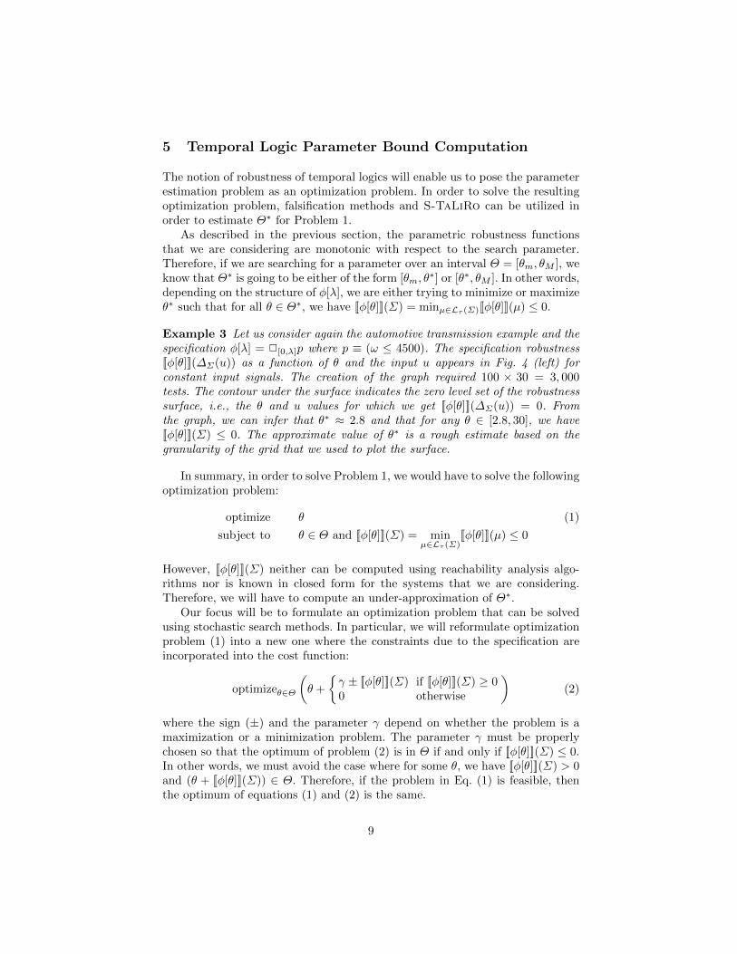
Example 3 Let us consider again the automotive transmission example and thespecification φ[λ] = 2[0,λ]p where p ≡ (ω ≤ 4500). The specification robustness[[φ[θ]]](∆Σ(u)) as a function of θ and the input u appears in Fig. 4 (left) forconstant input signals. The creation of the graph required 100 × 30 = 3, 000tests. The contour under the surface indicates the zero level set of the robustnesssurface, i.e., the θ and u values for which we get [[φ[θ]]](∆Σ(u)) = 0. Fromthe graph, we can infer that θ∗ ≈ 2.8 and that for any θ ∈ [2.8, 30], we have[[φ[θ]]](Σ) ≤ 0. The approximate value of θ∗ is a rough estimate based on thegranularity of the grid that we used to plot the surface.

In summary, in order to solve Problem 1, we would have to solve the followingoptimization problem:

optimize θ (1)

subject to θ ∈ Θ and [[φ[θ]]](Σ) = minµ∈Lτ (Σ)

[[φ[θ]]](µ) ≤ 0

However, [[φ[θ]]](Σ) neither can be computed using reachability analysis algo-rithms nor is known in closed form for the systems that we are considering.Therefore, we will have to compute an under-approximation of Θ∗.

Our focus will be to formulate an optimization problem that can be solvedusing stochastic search methods. In particular, we will reformulate optimizationproblem (1) into a new one where the constraints due to the specification areincorporated into the cost function:

optimizeθ∈Θ

(θ +

{γ ± [[φ[θ]]](Σ) if [[φ[θ]]](Σ) ≥ 00 otherwise

)(2)

where the sign (±) and the parameter γ depend on whether the problem is amaximization or a minimization problem. The parameter γ must be properlychosen so that the optimum of problem (2) is in Θ if and only if [[φ[θ]]](Σ) ≤ 0.In other words, we must avoid the case where for some θ, we have [[φ[θ]]](Σ) > 0and (θ + [[φ[θ]]](Σ)) ∈ Θ. Therefore, if the problem in Eq. (1) is feasible, thenthe optimum of equations (1) and (2) is the same.

9

5.1 Non-increasing Robustness Functions

First, we consider the case of non-increasing robustness functions [[φ[θ]]](Σ) withrespect to the search variable θ. In this case, the optimization problem is aminimization problem.

To see why this is the case, assume that [[φ[θM ]]](Σ) ≤ 0. Since for θ ≤ θM ,we have [[φ[θ]]](Σ) ≥ [[φ[θM ]]](Σ), we need to find the minimum θ such that westill have [[φ[θ]]](Σ) ≤ 0. That θ will be θ∗ since for all θ′ ∈ [θ∗, θM ], we will have[[φ[θ′]]](Σ) ≤ 0.

We will reformulate the problem of Eq. (2) so that we do not have to solvetwo separate optimization problems. From (2), we have:

minθ∈Θ

(θ +

{γ + minµ∈Lτ (Σ)[[φ[θ]]](µ) if minµ∈Lτ (Σ)[[φ[θ]]](µ) ≥ 00 otherwise

)=

= minθ∈Θ

(θ + min

µ∈Lτ (Σ)

{γ + [[φ[θ]]](µ) if [[φ[θ]]](µ) ≥ 00 otherwise

)=

= minθ∈Θ

minµ∈Lτ (Σ)

(θ +

{γ + [[φ[θ]]](µ) if [[φ[θ]]](µ) ≥ 00 otherwise

)(3)

where γ ≥ max(θM , 0).The previous discussion is formalized in the following result.

Proposition 3 Let θ∗ and µ∗ be the parameters returned by an optimizationalgorithm that is applied to the problem in Eq. (3). If [[φ[θ∗]]](µ∗) ≤ 0, then forall θ ∈ Θ∗ = [θ∗, θM ], we have [[φ[θ]]](Σ) ≤ 0.

Proof. If [[φ[θ∗]]](µ∗) ≤ 0, then [[φ[θ∗]]](Σ) ≤ 0. Since [[φ[θ]]](Σ) is non-increasingwith respect to θ, then for all θ ∈ [θ∗, θM ], we also have [[φ[θ]]](Σ) ≤ 0.

Since we are utilizing stochastic optimization methods [7, 10, 8, 4] to solveproblem (3), if [[φ[θ∗]]](µ∗) > 0, then we cannot infer that the system is correctfor all parameter values in Θ.

Example 4 Using Eq. (3) as a cost function, we can now compute the opti-mal parameter for Example 3 using our toolbox S-TaLiRo [10]. In particular,using Simulated Annealing as a stochastic optimization function, S-TaLiRo re-turns θ∗ ≈ 2.45 as optimal parameter for constant input u(t) = 99.8046. Thecorresponding temporal logic robustness for the specification 2[0,2.45](ω ≤ 4500)is −0.0445. The total number of tests performed for this example was 500 and,potentially, the accuracy of estimating θ∗ can be improved if we increase themaximum number of tests. However, we remark that based on several tests thealgorithm converges to a good approximation within 200 tests.

5.2 Non-decreasing Robustness Functions

The case of non-decreasing robustness functions is symmetric to the case ofnon-increasing robustness functions. In particular, the optimization problem is

10

a maximization problem. We will reformulate the problem of Eq. (2) so that wedo not have to solve two separate optimization problems. From (2), we have:

maxθ∈Θ

(θ +

{γ −minµ∈Lτ (Σ)[[φ[θ]]](µ) if minµ∈Lτ (Σ)[[φ[θ]]](µ) ≥ 00 otherwise

)=

= maxθ∈Θ

(θ +

{γ + maxµ∈Lτ (Σ) (−[[φ[θ]]](µ)) if maxµ∈Lτ (Σ) (−[[φ[θ]]](µ)) ≤ 00 otherwise

)=

= maxθ∈Θ

(θ + max

µ∈Lτ (Σ)

{γ − [[φ[θ]]](µ) if − [[φ[θ]]](µ) ≤ 00 otherwise

)=

= maxθ∈Θ

maxµ∈Lτ (Σ)

(θ +

{γ − [[φ[θ]]](µ) if [[φ[θ]]](µ) ≥ 00 otherwise

)(4)

where γ ≤ min(θm, 0).

The previous discussion is formalized in the following result.

Proposition 4 Let θ∗ and µ∗ be the parameters returned by an optimizationalgorithm that is applied to the problem in Eq. (4). If [[φ[θ∗]]](µ∗) ≤ 0, then forall θ ∈ Θ∗ = [θm, θ

∗], we have [[φ[θ]]](Σ) ≤ 0.

Proof. If [[φ[θ∗]]](µ∗) ≤ 0, then [[φ[θ∗]]](Σ) ≤ 0. Since [[φ[θ]]](Σ) is non-decreasingwith respect to θ, then for all θ ∈ [θm, θ

∗], we also have [[φ[θ]]](Σ) ≤ 0.

Again, if [[φ[θ∗]]](µ∗) > 0, then we cannot infer that the system is correct forall parameter values in Θ.

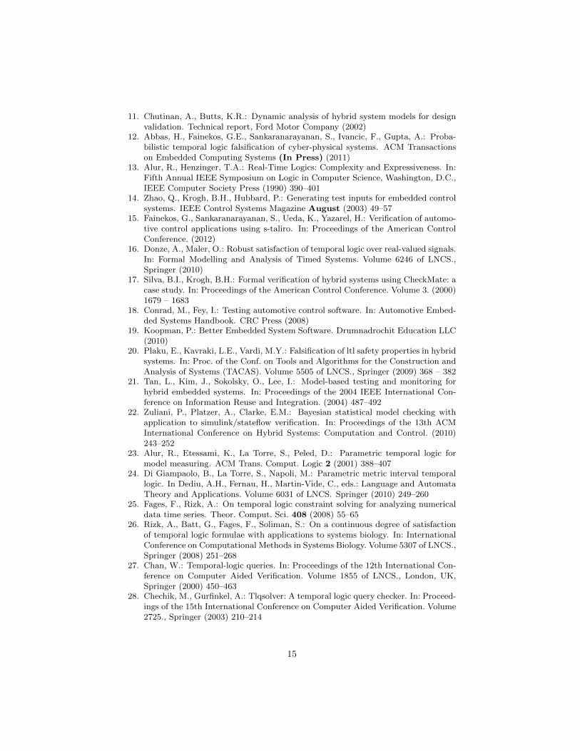
Example 5 Let us consider the specification φ[λ] = 2[λ,30](ω ≤ 4500) on ourrunning example. The specification robustness [[φ[θ]]](∆Σ(u)) as a function of θand the input u appears in Fig. 5 (left) for constant input signals. The creationof the graph required 100 × 30 = 3, 000 tests. The contour under the surfaceindicates the zero level set of the robustness surface, i.e., the θ and u valuesfor which we get [[φ[θ]]](∆Σ(u)) = 0. We remark that the contour is actually anapproximation of the zero level set computed by a linear interpolation using theneighboring points on the grid. From the graph, we could infer that θ∗ ≈ 13.8 andthat for any θ ∈ [0, 13.8], we would have [[φ[θ]]](Σ) ≤ 0. Again, the approximatevalue of θ∗ is a rough estimate based on the granularity of the grid.

Using Eq. (4) as a cost function, we can now compute the optimal parameterfor Example 3 using our toolbox S-TaLiRo [10]. S-TaLiRo returns θ∗ ≈ 12.59as optimal parameter for constant input u(t) = 90.88 within 250 tests. Thetemporal logic robustness for the specification 2[12.59,30](ω ≤ 4500) with respectto the input u appears in Fig. 5 (right). Some observations: (i) The θ∗ ≈ 12.59computed by S-TaLiRo is actually very close to the optimal value since forθ∗ ≈ 12.79 the system does not falsify any more. (ii) The systematic testing thatwas used in order to generate the graph was not able to accurately compute a goodapproximation to the parameter unless even more tests (> 3000) are generated.

11

6 Experiments and a Case Study

The parametric MTL exploration of embedded systems was motivated by a chal-lenge problem published by Ford in 2002 [11]. In particular, the report provideda simple – but still realistic – model of a powertrain system (both the physicalsystem and the embedded control logic) and posed the question whether thereare constant operating conditions that can cause a transition from gear two togear one and then back to gear two. Such a sequence would imply that thetransition was not necessary in the first place.

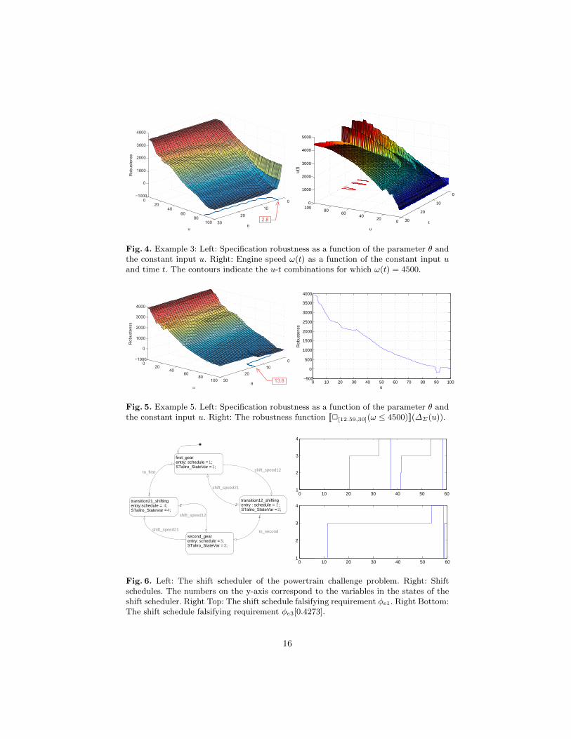
The system is modeled in Checkmate [17]. It has 6 continuous state variablesand 2 Stateflow charts with 4 and 6 states, respectively. The Stateflow chart forthe shift scheduler appears in Fig. 6. The system dynamics and switching condi-tions are linear. However, some switching conditions depend on the inputs to thesystem. The latter makes the application of standard hybrid system verificationtools not a straightforward task.

In [15], we demonstrated that S-TaLiRo [10] can successfully solve the chal-lenge problem (see Fig. 6) by formalizing the requirement as an MTL specifica-tion φe1 = ¬3(g2 ∧3(g1 ∧3g2)) where gi is a proposition that is true when thesystem is in gear i. Stochastic search methods can be applied to solve the result-ing optimization problem where the cost function is the robustness of the specifi-cation. Moreover, inspired by the success of S-TaLiRo on the challenge problem,we tried to ask a more complex question. Namely, does a transition exists fromgear two to gear one and back to gear two in less than 2.5 sec? An MTL specifi-cation that can capture this requirement is φe2 = 2((¬g1 ∧Xg1)→ 2[0,2.5]¬g2).

The natural question that arises is what would be the smallest time for whichsuch a transition can occur? We can formulate a parametric MTL formula toquery the model of the powertrain system: φe3[λ] = 2((¬g1∧Xg1)→ 2[0,λ]¬g2).We have extended S-TaLiRo to be able to handle parametric MTL specifica-tions. The total simulation time of the model was 60 sec and the search intervalwas Θ = [0, 30]. S-TaLiRo returned θ∗ ≈ 0.4273 as the minimum parameterfound (See Fig. 6) using about 300 tests of the system.

In Table 6, we present some experimental results. Since no other techniquecan solve the parameter estimation problem for MTL formulas over hybrid sys-tems, we compare our method with the falsification methods that we have devel-oped in the past [12, 7]. A detailed description of the benchmark problems canbe found in [12, 7] and the benchmarks can be downloaded with the S-TaLiRodistribution2. In order to be able to compare the two methods, when performingparameter estimation, we regard a parameter value less than the constant in theMTL formula as falsification. Notably, for benchmark problems that are easierto falsify, the parameter estimation method incurs additional cost in the sense ofreduced number of falsifications. On the other hand, on hard problem instances,the parameter estimation method provides us with parameter ranges for whichthe system fails the specification. Moreover, on the powertrain challenge prob-lem, the parameter estimation method actually helps in falsifying the system.

2 https://sites.google.com/a/asu.edu/s-taliro/

12

Table 1. Experimental Comparison of Falsification (FA) vs. Parameter Estimation(PE). Each instance was run for 100 times and each run was executed for a maximumof 1000 tests. Legend: #Fals.: the number of runs falsified, Parameter Estimate:〈min, average, max〉 of the parameter value computed, dnf : did not finish.

Benchmark Problem #Fals. Parameter Estimate

Specification Instance FA PE PE

φAT2 [λ] = ¬3(pAT1 ∧3[0,λ]pAT2 ) φAT2 [10] 96 84 〈7.7, 9.56, 16.84〉

φAT3 [λ] = ¬3(pAT1 ∧3[0,λ]pAT3 ) φAT3 [10] 51 0 〈10.00, 10.22, 14.66〉

φAT4 [λ] = ¬3(pAT1 ∧3[0,λ]pAT2 ) φAT4 [7.5] 0 0 〈7.57, 7.7, 8.56〉

φAT5 [λ] = ¬3(pAT1 ∧3[0,λ]pAT2 ) φAT5 [5] 0 0 〈7.56, 7.74, 9.06〉

φe3[2.5] dnf 93 〈1.28, 2.26, 6.82〉

We conjecture that the reason for this improved performance is that the timingrequirements on this problem are more important than the state constraints.

7 Related Work

The topic of testing embedded software and, in particular, embedded controlsoftware is a well studied problem that involves many subtopics well beyondthe scope of this paper. We refer the reader to specialized book chapters andtextbooks for further information [18, 19]. Similarly, a lot of research has beeninvested on testing methods for Model Based Development (MBD) of embeddedsystems [3]. However, the temporal logic testing of embedded and hybrid systemshas not received much attention [20, 21, 4, 22].

Parametric temporal logics were first defined over traces of finite state ma-chines [23]. In parametric temporal logics, some of the timing constraints of thetemporal operators are replaced by parameters. Then, the goal is to developalgorithms that will compute the values of the parameters that make the specifi-cation true under some optimality criteria. That line of work has been extendedto real-time systems and in particular to timed automata [24] and continuous-time signals [9]. The authors in [25, 26] define a parametric temporal logic calledquantifier free LTL over real valued signals. However, they focus on the problemof determining system parameters such that the system satisfies a given propertyrather than on the problem of exploring the properties of a given system.

Another related research topic is the problem of Temporal Logic Queries [27,28]. In detail, given a model of the system and a temporal logic formula φ, asubformula in φ is replaced with a special symbol ?. Then, the problem is todetermine a set of Boolean formulas such that if these formulas are placed intothe placeholder ?, then φ holds on the model.

8 Conclusions

An important stage in Model Based Development (MBD) of embedded controlsoftware is the formalization of system requirements. We advocate that Metric

13

Temporal Logic (MTL) is an excellent candidate for formalizing interesting de-sign requirements. In this paper, we have presented a solution on how we canexplore system properties using Parametric MTL (PMTL) [9]. Based on thenotion of robustness of MTL [6], we have converted the parameter estimationproblem into an optimization problem which we solve using S-TaLiRo [10].Even though this paper presents a method for estimating the range for a singleparameter, the results can be easily extended to multiple parameters as longas the robustness function has the same monotonicity with respect to all theparameters. Finally, we have demonstrated that the our method can provideinteresting insights to the powertrain challenge problem [11].

Acknowledgments This work was partially supported by a grant from the NSFIndustry/University Cooperative Research Center (I/UCRC) on Embedded Sys-tems at Arizona State University and NSF awards CNS-1116136 and CNS-1017074.

References

1. Lions, J.L., Lbeck, L., Fauquembergue, J.L., Kahn, G., Kubbat, W., Levedag, S.,Mazzini, L., Merle, D., O’Halloran, C.: Ariane 5, flight 501 failure, report by theinquiry board. Technical report, CNES (1996)

2. Hoffman, E.J., Ebert, W.L., Femiano, M.D., Freeman, H.R., Gay, C.J., Jones, C.P.,Luers, P.J., Palmer, J.G.: The near rendezvous burn anomaly of december 1998.Technical report, Applied Physics Laboratory, Johns Hopkins University (1999)

3. Tripakis, S., Dang, T.: Modeling, Verification and Testing using Timed and HybridAutomata. In: Model-Based Design for Embedded Systems. CRC Press (2009)383–436

4. Nghiem, T., Sankaranarayanan, S., Fainekos, G.E., Ivancic, F., Gupta, A., Pappas,G.J.: Monte-carlo techniques for falsification of temporal properties of non-linearhybrid systems. In: Proceedings of the 13th ACM International Conference onHybrid Systems: Computation and Control, ACM Press (2010) 211–220

5. Koymans, R.: Specifying real-time properties with metric temporal logic. Real-Time Systems 2 (1990) 255–299

6. Fainekos, G.E., Pappas, G.J.: Robustness of temporal logic specifications forcontinuous-time signals. Theoretical Computer Science 410 (2009) 4262–4291

7. Sankaranarayanan, S., Fainekos, G.: Falsification of temporal properties of hybridsystems using the cross-entropy method. In: ACM International Conference onHybrid Systems: Computation and Control. (2012)

8. Annapureddy, Y.S.R., Fainekos, G.E.: Ant colonies for temporal logic falsifica-tion of hybrid systems. In: Proceedings of the 36th Annual Conference of IEEEIndustrial Electronics. (2010) 91–96

9. Asarin, E., Donze, A., Maler, O., Nickovic, D.: Parametric identification of tempo-ral properties. In: Runtime Verification. Volume 7186 of LNCS., Springer (2012)147–160

10. Annapureddy, Y.S.R., Liu, C., Fainekos, G.E., Sankaranarayanan, S.: S-taliro: Atool for temporal logic falsification for hybrid systems. In: Tools and algorithms forthe construction and analysis of systems. Volume 6605 of LNCS., Springer (2011)254–257

14

11. Chutinan, A., Butts, K.R.: Dynamic analysis of hybrid system models for designvalidation. Technical report, Ford Motor Company (2002)

12. Abbas, H., Fainekos, G.E., Sankaranarayanan, S., Ivancic, F., Gupta, A.: Proba-bilistic temporal logic falsification of cyber-physical systems. ACM Transactionson Embedded Computing Systems (In Press) (2011)

13. Alur, R., Henzinger, T.A.: Real-Time Logics: Complexity and Expressiveness. In:Fifth Annual IEEE Symposium on Logic in Computer Science, Washington, D.C.,IEEE Computer Society Press (1990) 390–401

14. Zhao, Q., Krogh, B.H., Hubbard, P.: Generating test inputs for embedded controlsystems. IEEE Control Systems Magazine August (2003) 49–57

15. Fainekos, G., Sankaranarayanan, S., Ueda, K., Yazarel, H.: Verification of automo-tive control applications using s-taliro. In: Proceedings of the American ControlConference. (2012)

16. Donze, A., Maler, O.: Robust satisfaction of temporal logic over real-valued signals.In: Formal Modelling and Analysis of Timed Systems. Volume 6246 of LNCS.,Springer (2010)

17. Silva, B.I., Krogh, B.H.: Formal verification of hybrid systems using CheckMate: acase study. In: Proceedings of the American Control Conference. Volume 3. (2000)1679 – 1683

18. Conrad, M., Fey, I.: Testing automotive control software. In: Automotive Embed-ded Systems Handbook. CRC Press (2008)

19. Koopman, P.: Better Embedded System Software. Drumnadrochit Education LLC(2010)

20. Plaku, E., Kavraki, L.E., Vardi, M.Y.: Falsification of ltl safety properties in hybridsystems. In: Proc. of the Conf. on Tools and Algorithms for the Construction andAnalysis of Systems (TACAS). Volume 5505 of LNCS., Springer (2009) 368 – 382

21. Tan, L., Kim, J., Sokolsky, O., Lee, I.: Model-based testing and monitoring forhybrid embedded systems. In: Proceedings of the 2004 IEEE International Con-ference on Information Reuse and Integration. (2004) 487–492

22. Zuliani, P., Platzer, A., Clarke, E.M.: Bayesian statistical model checking withapplication to simulink/stateflow verification. In: Proceedings of the 13th ACMInternational Conference on Hybrid Systems: Computation and Control. (2010)243–252

23. Alur, R., Etessami, K., La Torre, S., Peled, D.: Parametric temporal logic formodel measuring. ACM Trans. Comput. Logic 2 (2001) 388–407

24. Di Giampaolo, B., La Torre, S., Napoli, M.: Parametric metric interval temporallogic. In Dediu, A.H., Fernau, H., Martin-Vide, C., eds.: Language and AutomataTheory and Applications. Volume 6031 of LNCS. Springer (2010) 249–260

25. Fages, F., Rizk, A.: On temporal logic constraint solving for analyzing numericaldata time series. Theor. Comput. Sci. 408 (2008) 55–65

26. Rizk, A., Batt, G., Fages, F., Soliman, S.: On a continuous degree of satisfactionof temporal logic formulae with applications to systems biology. In: InternationalConference on Computational Methods in Systems Biology. Volume 5307 of LNCS.,Springer (2008) 251–268

27. Chan, W.: Temporal-logic queries. In: Proceedings of the 12th International Con-ference on Computer Aided Verification. Volume 1855 of LNCS., London, UK,Springer (2000) 450–463

28. Chechik, M., Gurfinkel, A.: Tlqsolver: A temporal logic query checker. In: Proceed-ings of the 15th International Conference on Computer Aided Verification. Volume2725., Springer (2003) 210–214

15

010

20

30

020

4060

80100

−1000

0

1000

2000

3000

4000

θu

Robustenss

2.8 020

4060

80100

0

10

20

30

0

1000

2000

3000

4000

5000

t

u

ω(t

)

Fig. 4. Example 3: Left: Specification robustness as a function of the parameter θ andthe constant input u. Right: Engine speed ω(t) as a function of the constant input uand time t. The contours indicate the u-t combinations for which ω(t) = 4500.

010

2030

020

4060

80100

−1000

0

1000

2000

3000

4000

θu

Robustenss

13.8 0 10 20 30 40 50 60 70 80 90 100−500

0

500

1000

1500

2000

2500

3000

3500

4000

u

Rob

uste

nss

Fig. 5. Example 5. Left: Specification robustness as a function of the parameter θ andthe constant input u. Right: The robustness function [[2[12.59,30](ω ≤ 4500)]](∆Σ(u)).

first_gearentry: schedule =1;STaliro_StateVar = 1;

transition12_shiftingentry : schedule = 2;STaliro_StateVar = 2;

transition21_shiftingentry:schedule = 4;STaliro_StateVar = 4;

second_gearentry: schedule =3;STaliro_StateVar = 3;

to_first

1

shift_speed12

shift_speed21

2

shift_speed12

2

to_second

1

shift_speed21

0 10 20 30 40 50 601

2

3

4

0 10 20 30 40 50 601

2

3

4

Fig. 6. Left: The shift scheduler of the powertrain challenge problem. Right: Shiftschedules. The numbers on the y-axis correspond to the variables in the states of theshift scheduler. Right Top: The shift schedule falsifying requirement φe1. Right Bottom:The shift schedule falsifying requirement φe3[0.4273].

16