QUCEH WORKING PAPER SERIES

http://www.quceh.org.uk/working-papers

RISE AND FALL IN THE THIRD REICH:

SOCIAL MOBILITY AND NAZI MEMBERSHIP

Matthias Blum (Queen’s University Belfast)

Alan de Bromhead (Queen’s University Belfast)

Working Paper 2017-04

QUEEN’S UNIVERSITY CENTRE FOR ECONOMIC HISTORY

Queen’s University Belfast

185 Stranmillis Road

Belfast BT9 5EE

April 2017

Rise and Fall in the Third Reich:

Social Mobility and Nazi Membership

Matthias Blum∗

Alan de Bromhead†

Abstract

This paper explores the relationship between Nazi membership and

social mobility using a unique and highly detailed dataset of military con-

scripts and volunteers during the Third Reich. We find that membership of

a Nazi organisation is positively related to social mobility when measured

by the difference between fathers’ and sons’ occupations. This relationship

is stronger for the more ‘elite’ NS organisations, the NSDAP and the SS.

However, we find that this observed difference in upward mobility is driven

by individuals with different characteristics self-selecting into these organ-

isations, rather than from a direct reward to membership. These results

are confirmed by a series of robustness tests. In addition, we employ our

highly-detailed dataset to explore the determinants of Nazi membership.

We find that NS membership is associated with higher socio-economic

background and human capital levels.

JEL Codes: J62; N24; N44; P16

Keywords: National Socialism; Third Reich; Social Mobility; Nazi

Membership; Second World War; Political Economy; Germany; Eco-

nomic History

∗Queen’s University Belfast and QUCEH, Queen’s Management School, Riddel Hall,185 Stranmillis Road, Belfast, Northern Ireland, BT9 5EE, United Kingdom. (e-mail:matthias.blum@qub.ac.uk)†Queen’s University Belfast and QUCEH, Queen’s Management School, Riddel Hall,

185 Stranmillis Road, Belfast, Northern Ireland, BT9 5EE, United Kingdom. (e-mail:a.debromhead@qub.ac.uk)

1

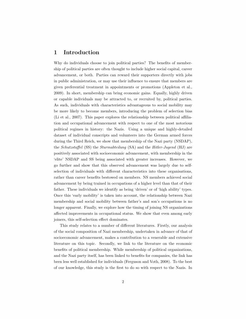
1 Introduction

Why do individuals choose to join political parties? The benefits of member-

ship of political parties are often thought to include higher social capital, career

advancement, or both. Parties can reward their supporters directly with jobs

in public administration, or may use their influence to ensure that members are

given preferential treatment in appointments or promotions (Appleton et al.,

2009). In short, membership can bring economic gains. Equally, highly driven

or capable individuals may be attracted to, or recruited by, political parties.

As such, individuals with characteristics advantageous to social mobility may

be more likely to become members, introducing the problem of selection bias

(Li et al., 2007). This paper explores the relationship between political affilia-

tion and occupational advancement with respect to one of the most notorious

political regimes in history: the Nazis. Using a unique and highly-detailed

dataset of individual conscripts and volunteers into the German armed forces

during the Third Reich, we show that membership of the Nazi party (NSDAP),

the Schutzstaffel (SS) the Sturmabteilung (SA) and the Hitler-Jugend (HJ) are

positively associated with socioeconomic advancement, with membership in the

‘elite’ NSDAP and SS being associated with greater increases. However, we

go further and show that this observed advancement was largely due to self-

selection of individuals with different characteristics into these organisations,

rather than career benefits bestowed on members. NS members achieved social

advancement by being trained in occupations of a higher level than that of their

father. These individuals we identify as being ‘driven’ or of ‘high ability’ types.

Once this ‘early mobility’ is taken into account, the relationship between Nazi

membership and social mobility between father’s and son’s occupations is no

longer apparent. Finally, we explore how the timing of joining NS organizations

affected improvements in occupational status. We show that even among early

joiners, this self-selection effect dominates.

This study relates to a number of different literatures. Firstly, our analysis

of the social composition of Nazi membership, undertaken in advance of that of

socioeconomic advancement, makes a contribution to a venerable and extensive

literature on this topic. Secondly, we link to the literature on the economic

benefits of political membership. While membership of political organizations,

and the Nazi party itself, has been linked to benefits for companies, the link has

been less well established for individuals (Ferguson and Voth, 2008). To the best

of our knowledge, this study is the first to do so with respect to the Nazis. In

2

addition, our work is linked to studies of social mobility more generally, as our

analysis identifies determinants of social mobility beyond political connections.

What are the economic benefits of connections to political organizations? A

number of studies have identified the benefits to companies of political connec-

tions (Fisman (2001); Faccio (2006); Claessens et al. (2008); Acemoglu et al.

(2013)). In the context of Nazi Germany, Ferguson and Voth (2008) estimated

that companies connected to the Nazi party outperformed their unconnected

competitors by 5% to 8% in terms of returns. The benefits to individuals stem-

ming from political connections are perhaps less well explored. Establishing a

causal link running from party membership to economic benefits is also difficult

due to omitted variable bias, as high-ability or ‘driven’ individuals may be more

likely to establish links to a political party. A study by Li et al. (2007) attempts

to overcome this bias by examining the relationship between Communist Party

membership and earnings of twins in China. The authors find, after control-

ling for a twin fixed effect, that the positive relationship between earnings and

membership disappears, leading them to conclude that individuals with superior

abilities joined the party, not that party members benefit from their political

position. Likewise, Gerber (2000) finds that former Communist Party mem-

bers in post-transition Russia had higher earnings, but that this was driven by

the selection of individuals with advantageous, but unobservable, traits (such

as ambition) into the party. Nonetheless, other studies of connections to the

Chinese Communist Party membership by Appleton et al. (2009) and Li et al.

(2012) do not find selectivity to be a serious problem, suggesting a causal effect

of membership on earnings.

In this paper we examine whether Nazi membership was associated with so-

cioeconomic advancement and explore whether membership was directly linked

to advancement, or if individuals with different attributes selected into the party.

This analyis is possible due to the availability of detailed individual level data on

German soldiers during the period 1936-1945. We go further and examine the

relationship for four categories of National Socialist organizations: the NSDAP

(Nazi Party), the Schutzstaffel (SS), the Sturmabteilung (SA) and the Hitler-

Jugend (HJ). In this way we capture a broader picture of Nazi organizations

and the characteristics of membership and explore differnces between memer-

ship of the ‘elite’ NS movements, the NSDAPand the SS, and the mass youth

movement of the Hitler-Jugend. Before looking at the benefits of membership

of these various NS organizations, we first explore the determinants of being

a member of each organization and attempt to address the question of ‘who

3

joined the Nazis?’ Our dataset provides a rare opportunity to examine Nazi

members relative to the rest of the population. Analysis of party member lists

can give you an indication of the social background of Nazi Party members, but

by definition omits those who never joined. The party member lists, such as

those formerly held at the Berlin Data Centre (BDC), also lack detailed infor-

mation on education and family background, important variables to consider

when analysing social class (Muhlberger, 1991, p.25), information that is avail-

able from our sample. In addition, as previously highlighted, we can exploit

these data to examine memberships of different types of NS organisations and

not just the Nazi Party itself (NSDAP).

The analysis will proceed as follows: the next section provides a brief review

of the literature on support for the Nazis andand establishes the hypotheses

to be tested, while the third section describes the data used in the analysis.

Section four analyses the determinants of NS membership before the relationship

between social mobility and membership are explored. Section five tests the

robustness of our findings before the final section concludes.

2 The Nazis and Social Background

Understanding what motivated millions of ordinary Germans to support the

Nazi party has been the goal of historians and political scientists for decades

(inter alia Lipset (1960); Hamilton (1982); Childers (1983); Falter (1991)). The

various explanations proposed generally fall under one of a small number of

broad categories. Firstly, there are the theories that focus on the appeal of the

Nazi party to certain sections of society (King et al., 2008). These ‘group-based’

theories include those that consider the Nazi appeal to have been greatest among

those on the fringes of society, typically non-voters, who felt marginalised within

the Weimar system (Bendix, 1952). This theory has recently been challenged

however by Satyanath et al. (2013), who argue that a vibrant networks of clubs

and associations in Weimar Germany facilitated the rise of the party: high social

capital, not low social capital, paved the way for the Nazis. Other group-theories

emphasise the Nazis’ disproportionate popularity among certain social classes.

The social-class theory is perhaps the most venerable and persistent, beginning

with the work of Seymour Lipset, who identified the typical Nazi voter in 1932

as

“a middle-class self-employed Protestant who lived either on a farm

4

or in a small community, and who had previously voted for a cen-

trist or regionalist political party strongly opposed to the power and

influence of big business and big labor.” (Lipset, 1960, p. 149)

That the Nazis were predominantly a lower middle-class party is also argued

by Michael Kater in his analysis of party membership (Kater, 1983). This

hypothesis is far from being universally accepted however and is opposed by

Hamilton (1982), who argues that disproportionately high support for the Nazis

was an upper-middle and upper-class phenomenon, as well as by Madden (1987),

who highlights the diverse social background of party members. Perhaps the

only group for which there is a near consensus regarding support for the Nazis

is Catholics: consistently, Catholics appear to have been less likely to vote for

the NSDAP or to become members of the party (inter alia Childers (1983);

King et al. (2008); Satyanath et al. (2013)). The other main view of Nazi party

support is that the NSDAP were not just a party which appealed to particular

groups, but were rather a ‘catchall party of protest’ which drew support from all

sections of society (Childers, 1983). The view that the Nazis were a mass-party

with widespread appeal is perhaps most associated with Jurgen Falter, who

argues that class or confession based theories can only go so far in explaining

support for the Nazis and that the Nazis received support from across the social

spectrum must be acknowledged (Falter, 2000). Following this line of reasoning,

King et al. (2008) combine the ‘catch-all’ theory and the ‘group-theory’ in their

analysis of Nazi voting and find that, although there was a general swing towards

the Nazi party across all social groups, the party achieved disproportionately

high support support among the ‘working-poor’: those not directly under threat

of unemployment but nonetheless negatively affected by the recession of the early

1930s.

More recently, in keeping with the mass-support theories, the rational, eco-

nomic self-interest of individuals has been highlighted as an explanation for sup-

porting the Nazis, either electorally or by joining the party itself. According to

Brustein (1998), individuals will support a party if the benefits to supporting the

party outweigh the costs. With respect to the Nazi party membership between

1925 and 1933, Brustein argues that those individuals whose material interests

were aligned with the party’s platform were more likely to become members. In

particular, he highlights the ability of the party to recruit successfully among

the ‘old middle-class’, blue-collar workers in import-orientated industries and

male, married white-collar workers and concludes that these groups’ interests

5

were closely aligned with Nazi party programs. Building on Brustein’s analysis,

Ault (2002) concludes that material reasons for joining the party became pre-

dominant only perhaps from 1930 onward and that non-material interests, or

‘identity politics’ better explains membership in the early years of the party.

3 Data

The dataset employed in the analysis of NS membership and social mobil-

ity was constructed from a sample drawn from non-commissioned officers and

lower ranked soldiers serving in the German armed forces during the Second

World War over the period 1936-1945. In total, a representative sample from 68

companies was constructed, comprising of units of all branches of the German

armed forces, most of which served in the army (Heer). Additionally, informa-

tion about members of the Air Force (Luftwaffe), Waffen-SS, and non-German

soldiers (mostly Eastern Belgians, Austrians, Luxembourger and French from

Alsace-Lorraine) were compiled.1 The sample is drawn from the former military

district VI (Wehrkreis VI) in modern-day North Rhine-Westphalia and Lower

Saxony (Rass (2001); Rass (2003, p.54ff)). The information in this sample

were compiled from the following sources and agencies: the WASt (Wehrmach-

tauskunftstelle fur Kriegsverluste und Kriegsgefangene), the agency responsible

for compiling information on soldiers who were killed or were taken prisoner,

and the BA-ZNS (Bundesarchiv-Zentralnachweisstelle), responsible for adminis-

tering personal information about soldiers. This material was complemented by

information on soldiers provided by the Red Cross’s Tracing Service and a cen-

tral register on repatriated soldiers returning from war captivity (Rass (2001);

Rass (2003, p.61ff)).2 The dataset comprises detailed personal information on

each individual soldier, such as date of medical examination, information about

family history, such as year of death of parents, place and date of birth, and

religion, as well as information about an individual’s socioeconomic background,

as recorded on the date of enlistment. The descriptive statistics for the sample

used in the analysis are given in Table 1.

From the information contained in the sample, we can determine the occupa-

tion an individual is trained for, the occupation actually practiced at the time

1The overwhelming majority of our sample were conscripts, with less than 7% being vol-unteers.

2The authors thank Christoph Rass for valuable information on the data set as well as theLeibniz-Institut fur Sozialwissenschaften (GESIS) for providing the data set.

6

Table 1: DESCRIPTIVE STATISTICS

(1) (2) (3) (4) (5)

VARIABLES N mean sd min max

NSDAP member 13,962 0.0212 0.144 0 1

SS member 13,962 0.0198 0.139 0 1

SA member 13,962 0.0654 0.247 0 1

Hitler Youth member 13,962 0.348 0.476 0 1

Other NS member 13,962 0.0514 0.221 0 1

Roman Catholic 13,962 0.547 0.498 0 1

Year of birth 13,962 1916 7.055 1900 1929

Occupation Father 12,957 2.721 0.780 1 5

Occupation Trained 10,750 2.600 0.831 1 5

Occupation Practiced 10,753 2.633 0.789 1 5

Occupation (Father) - Low 12,957 0.423 0.494 0 1

Occupation (Father) - Middle 12,957 0.428 0.495 0 1

Occupation (Father) - High 12,957 0.149 0.356 0 1

Schooling - None 13,962 0.0163 0.126 0 1

Schooling - Low 13,962 0.572 0.495 0 1

Schooling - Middle 13,962 0.122 0.328 0 1

Schooling - High 13,962 0.0586 0.235 0 1

Schooling - Unknown 13,962 0.231 0.421 0 1

Urban - Pop. up to 2000 13,962 0.466 0.499 0 1

Urban - Pop. up to 10000 13,962 0.128 0.334 0 1

Urban - Pop. up to 50000 13,962 0.170 0.375 0 1

Urban - Pop. over 50000 13,962 0.236 0.425 0 1

Age at Examination 13,962 22.86 6.509 16 45

Volunteer 13,962 0.0657 0.248 0 1

Social Mobility Score 10,000 -0.0194 0.913 -4 4

Social Climb 10,000 0.271 0.445 0 1

Social Fall 10,000 0.263 0.440 0 1

No Social Climb or Fall 10,000 0.466 0.499 0 1

Large Social Climb 10,000 0.0315 0.175 0 1

Large Social Fall 10,000 0.0557 0.229 0 1

Higher Training Mobility 9,994 -0.0582 0.945 -4 3

Higher Job Mobility 9,550 0.0614 0.578 -3 4

7

of medical examination, and the occupation of an individual’s father. These

rich data allow us to investigate the link between socioeconomic background

and the membership of an NS organization, as well as the relationship between

membership and career advancement. Ideally, information on an individual’s

earnings would have been included but unfortunately this was not available.

We use information on socioeconomic background to categorise all individuals

using the Armstrong (1972) taxonomy, using occupational titles to differentiate

between professionals (e.g. doctors), semi-professionals (e.g. teachers), skilled

(e.g. tailors), semi-skilled (e.g. factory worker), and unskilled workers (e.g.

labourers). Each category is rank-ordered; unskilled workers are given a rank

of 1 while professionals are given a rank of 5.3 The dataset also provides infor-

mation regarding an individual’s educational background. The German school

system traditionally distinguished between three different school tracks: basic

school education, a medium degree school track and an advanced school track

which aims at preparing students for an academic education at college or univer-

sity. We use this three-tier scheme and categorise all individuals in the dataset

accordingly. This methodology allows grouping individuals into four categories:

the aforementioned school tracks serve as three broad categories, while one cat-

egory is generated to identify individuals without school-leaving qualifications.4

Variables reflecting additional individual characteristics, such as religion, age,

and place of habitation are also included, as can be seen in Table 1.

This dataset offers a unique set of opportunities that make this study worth-

while: first, our sample of German armed forces during the Second World War

allows us to compare members and non-members of a set of Nazi organiza-

tions and assess their differences with respect to socioeconomic characteristics.

Second, the data contain information about an individual’s education and oc-

cupation in addition to father’s occupation, providing a rare opportunity to

assess the role of education, societal background and intergenerational mobility

in detail. Third, the data allow us to assess membership in the following orga-

nizations separately: Nationalsozialistische Deutsche Arbeiterpartei (NSDAP),

the official political party of the Nazis; Sturmabteilung (SA) and Schutzstaffel

(SS), two major paramilitary organizations of the NSDAP; and the Hitlerjugend

(HJ), initially the youth organization of the NSDAP and after 1933, an amal-

3Farmers are included in category 3 with skilled workers. Excluding farmers from theanalysis does not materially affect the results.

4Individuals that were missing observations were included in a separate educational cate-gory “unknown”.

8

gam of formerly independent youth organizations. In doing so we can uncover

whether membership of ‘elite’ NS organisations, such as the NSDAP and SS,

was different to membership of less selective organisations, such as the SA and

HJ.

It is also important to discuss the issue of potential sample selection and

the implications this may have for the external validity of the results. Firstly,

military samples have been criticised as being unrepresentative of the general

population, and that endogenous selection often occurs (Bodenhorn et al., 2015).

The concern primarily relates to volunteer armies, the decision to enlist can

be related to personal characteristics and labour market potential. As this

labour market potential is likely to be related to cyclical economic conditions, a

selection effect may result in those with the poorest prospects deciding to enlist

while those with better prospects remain in the labour market. As a result,

any sample of volunteers is non-random. As Bodenhorn et al. (2015) suggest,

this selection effect is not apparent in samples of conscript armies, such as that

analysed in this paper 5. Furthermore, the fact that Germany mobilised for

“total war” during the 1940s ensured that many more individuals, of various

ages and backgrounds, were conscripted than would ordinarily be the case in

conscript army. As such some 12.5 million men served in the German armed

forces over the course of the war, relative to a male population aged 15-44 of

around 16.5 million in 1939 (Parrish and Marshall, 1978; Mitchell, 1998).

Inherent in the sample is that NSDAP membership will be underestimated

if higher-ranking party members were less likely to serve as regular soldiers

and more likely to enter the armed forces as officers. However, this is likely

to bias downwards the estimated influence of membership on social mobility if

relatively “less-able” party members are the type that we capture in this sample.

This limits what we are able to say about the higher ranking members of NS

organisations but helps to identify the influence among the “rank and file”.

Finally, it is acknowledged that for most individuals in the sample, we mea-

sure social mobility at the early stage of an individual’s career trajectory and

not total or lifetime mobility. For this reason we concentrate on diffences in

observed, albeit partially realised, intergenrational mobility between members

of NS organisations and non-members.

5Of course some individuals may have been able, or indeed some more able than others, toavoid or delay conscription.

9

4 Analysis

4.1 Membership of NS Organisations

Our analysis is divided into two parts. In a first step we run a set of logistic

regressions to assess correlates of membership in an NS organisation. The data

provide information on an individual’s membership in the following Nazi organ-

isations: NSDAP; SA; SS; and Hitler Youth. This level of detail allows us to

assess the socioeconomic composition of supporters of the NS regime in great

detail. These different groups represented different branches of the NS organisa-

tion. NSDAP membership reflects a direct political dimension while examining

SA and SS memberships allow insights into the factors fostering the likelihood of

joining a paramilitary organisation of the Nazi regime. A membership analysis

of the Hitler Youth allows a view of a different dimension of the Nazi organ-

isational structure: the collectivisation of youth organisations in Germany to

prepare young people to be loyal supporters of the regime. The decision to

join NSDAP, SS and SA was largely voluntary, while the Hitler Youth became

compulsory for all males aged 10-18 in 1939 (Lepage, 2008). We run several

logit regression models explaining each of the aforementioned memberships us-

ing different specifications to limit any biases arising from multicollinearity and

omitted variables, with the results shown in Table 2. We estimate

NSi = α+ βOccupationi + δSchoolingi + λReligioni + γXi + ε (1)

Where NSi reflects whether individual i is a member of an NS organisation.

By default, we control for an individual’s denomination to address the com-

mon finding in the literature that Catholics were less inclined to support NS

organisations.

As we would predict, being a member of the Roman Catholic Church re-

duces the likelihood of being a member of any NS organisation. In order to

capture social background or “class”, the occupation of an individual’s father is

included as an explanatory variable.6 All our models are designed as tests of

differences between a low occupational background and high and medium lev-

els, respectively. Generally, we find that individuals with higher occupational

backgrounds are more likely to be members of the NSDAP, SA, SS and Hitler

Youth. Exponentiating the coefficient in model 1 of Table 2 reveals that the

6As an alternative we included the individual’s practiced occupation. This generated verysimilar results.

10

Table 2: DETERMINANTS OF NS MEMBERSHIP

(1)

(2)

(3)

(4)

(5)

(6)

(7)

(8)

(9)

(10

)(1

1)

(12)

VA

RIA

BL

ES

NS

DA

PN

SD

AP

NS

DA

PS

AS

AS

AS

SS

SS

SH

JH

JH

J

Occ

upa

tio

na

l ba

ckg

round

Hig

h0.6

0***

0.4

1**

0.4

1**

0.3

5***

0.2

6**

0.2

6**

0.7

5***

0.6

7***

0.6

7***

0.5

4***

0.3

3***

0.3

2***

(3.2

0)

(2.0

5)

(2.0

5)

(2.9

9)

(2.1

3)

(2.1

3)

(3.8

0)

(3.2

8)

(3.2

8)

(6.1

3)

(3.5

1)

(3.4

8)

Med

ium

0.2

10.1

60.1

60.3

0***

0.2

8***

0.2

8***

0.5

8***

0.5

5***

0.5

5***

0.1

4**

0.0

80.0

9

(1.3

2)

(1.0

3)

(1.0

3)

(3.4

8)

(3.1

9)

(3.1

9)

(3.5

3)

(3.3

5)

(3.3

5)

(2.2

4)

(1.3

5)

(1.3

8)

Lo

wre

fere

nce

refe

renc

ere

fere

nce

refe

renc

ere

fere

nce

refe

renc

ere

fere

nce

refe

renc

ere

fere

nce

refe

renc

ere

fere

nce

refe

renc

e

Sch

oo

ling

lev

el

Hig

h1.4

71.4

61.6

2**

1.6

3**

0.7

00.7

01.3

2***

1.3

0***

(1.4

1)

(1.4

1)

(2.2

2)

(2.2

2)

(0.9

2)

(0.9

2)

(5.3

9)

(5.2

6)

Med

ium

1.5

31.5

31.5

7**

1.5

7**

0.2

90.2

90.7

7***

0.7

4***

(1.4

8)

(1.4

8)

(2.1

6)

(2.1

6)

(0.3

8)

(0.3

8)

(3.4

5)

(3.3

1)

Lo

w0.9

00.9

01.2

3*

1.2

3*

0.3

00.3

00.3

20.3

0

(0.8

8)

(0.8

8)

(1.7

2)

(1.7

2)

(0.4

1)

(0.4

1)

(1.5

1)

(1.4

3)

Unk

now

n0.2

10.2

01.4

5**

1.4

5**

0.0

90.0

90.4

2*

0.3

9*

(0.2

0)

(0.1

9)

(2.0

1)

(2.0

1)

(0.1

1)

(0.1

2)

(1.8

3)

(1.6

9)

No

nere

fere

nce

refe

renc

ere

fere

nce

refe

renc

ere

fere

nce

refe

renc

ere

fere

nce

refe

renc

e

Relig

ion

Ro

man

Cat

holic

-0.6

6*

**

-0.6

1*

**

-0.6

1*

**

-0.2

6*

**

-0.2

6*

**

-0.2

6*

**

-1.2

1**

*-1

.21*

**

-1.2

1*

**

-0.2

5**

*-0

.24*

**

-0.2

4*

**

(-3

.80)

(-3

.51)

(-3

.50)

(-2

.78)

(-2

.69)

(-2

.69)

(-6

.96)

(-6.9

5)

(-6.9

5)

(-3.6

4)

(-3

.53)

(-3

.42)

Pro

test

ant

refe

renc

ere

fere

nce

refe

renc

ere

fere

nce

refe

renc

ere

fere

nce

refe

renc

ere

fere

nce

refe

renc

ere

fere

nce

refe

renc

ere

fere

nce

Adm

itte

d a

s

Vo

lunt

eer

0.1

2-0

.04

-0.0

40.5

4***

(0.3

0)

(-0

.23)

(-0.1

3)

(4.8

2)

Dra

ftee

refe

renc

ere

fere

nce

refe

renc

ere

fere

nce

Co

ntr

ols

Yea

r o

r b

irth

YE

SY

ES

YE

SY

ES

YE

SY

ES

YE

SY

ES

YE

SY

ES

YE

SY

ES

Age

at m

edic

al e

xam

inat

ionY

ES

YE

SY

ES

YE

SY

ES

YE

SY

ES

YE

SY

ES

YE

SY

ES

YE

S

Urb

anis

atio

nY

ES

YE

SY

ES

YE

SY

ES

YE

SY

ES

YE

SY

ES

YE

SY

ES

YE

S

Dis

tric

t fix

ed e

ffec

tsY

ES

YE

SY

ES

YE

SY

ES

YE

SY

ES

YE

SY

ES

YE

SY

ES

YE

S

Ob

serv

atio

ns10,7

03

10,7

03

10,7

03

11,6

78

11,6

78

11,6

78

10,2

99

10,2

99

10,2

99

12,3

43

12,3

43

12,3

43

z-s

tatis

tics

in p

aren

thes

es,

***

p<

0.0

1,

** p

<0

.05,

* p

<0.1

11

odds of membership of the NSDAP were almost twice as high for those from

a high-status background relative to a low-status one. In addition to social

background, we also include information on the level of schooling to proxy the

educational status of an individual. We find a consistent pattern here. The

coefficients generally indicate that individuals with higher levels of educational

were more likely to be a member of any NS organisation. Whether the individ-

ual joined the German armed forces as a volunteer or was conscripted is also

included in the model. We do not find that those that volunteered for military

service were more likely to have been NSDAP, SA, or SS members. However,

there is a statistically significant difference with respect to the Hitler Youth;

individuals that volunteered for service in the German armed forces are found

to be more likely to have been members of the Hitler Youth compared to those

who did not volunteer. By default, all models control for an individual’s year

of birth and the year of medical examination. These variables constitute im-

portant control variables that capture any variation in membership that solely

reflects different stages on an individual’s educational or career ladder. As for

NSDAP, SA and SS, those individuals born earlier had had more opportunities

to join any of these parties prior to medical examination (cohort effect). Sim-

ilarly, it may be reasonable to assume that for more advanced careers, returns

to membership were higher. On the other hand, the same control variables

capture a different effect with respect to membership in Hitler Youth. Slightly

older individuals, or those who joined the armed forces early might have been

simply too old by the time of medical examination to have been a member of

the Nazis youth organisation. Accordingly, we find that birth year is positively

related to membership of the Hitler Youth, but negatively related to NSDAP,

SA and SS membership in general. Age at medical examination is positively

correlated with NSDAP membership and negatively correlated with SA, SS and

Hitler Youth membership. We do not find consistent results when we control

for the city size: the only noteworthy finding is that individuals from areas with

fewer than 2,000 inhabitants were more likely to join the SA (not reported in

tables).

How do our findings compare to that of the previous Nazi membership liter-

ature? The results indicate that NSDAP members were more highly educated

and held higher occupational status than non-members. Interestingly, higher

levels of education and social standing are also associated with membership of

other NS organisations, even the ‘proletarian’ SA (Stachura, 2014b, p.108). To

visually compare the social background of NS members to non-members in the

12

Figure 1: BACKGROUND OF NS MEMBERS v. NON-MEMBERS

(a) NSDAP0

1020

3040

Per

cent

Low Med HighFather’s Occupation

NSDAP Non−NSDAP

(b) SS

010

2030

4050

Per

cent

Low Med HighFather’s Occupation

SS Non−SS

(c) SA

010

2030

4050

Per

cent

Low Med HighFather’s Occupation

SA Non−SA

(d) Hitler Youth

010

2030

40P

erce

nt

Low Med HighFather’s Occupation

HJ Non−HJ

sample, four histograms are presented for each organisation (figure 1). Fig 1

(a) examines membership of NSDAP. This shows that higher occupations were

over represented in the party while lower occupations were underrepresented,

with a similar picture visible for the SS in fig 1 (b). Fig 1 (c) confirms that

lower occupations were better represented among SA members but were under-

represented nonetheless. Not surprisingly the occupational background of HJ

members most closely matches that of non-members, although even here higher

level occupations are overrepresented (fig 1 (d)). Were the Nazis a ‘catch-all

party’ or an organisation of the elite? Our findings suggest that these defini-

tions are not mutually exclusive. Clearly the party managed to attract support

from all levels of society. However the goal of an organisation that mirrored

German society was not fully achieved: it is clear that higher-level occupations

were overrepresented in all NS organisations, even the in Hitler Youth.

13

4.2 Membership and Intergenerational Mobility

The next part of the analysis examines the relationship between membership of

NS organizations and social mobility. Did individuals benefit from membership

of these organizations? To determine this, we firstly construct a measure of

social mobility by comparing the occupation of an individual’s father to that

practiced by the son at the time of medical examination. Specifically, we take

the Armstrong category of the son’s occupation and subtract the corresponding

value for the father. For example, if an individual is in a category 4 (semi-

professional) occupation and their father had a category 2 occupation (semi-

skilled worker), then they would be assigned a social mobility score of two.7

As such, social mobility scores have a possible range of between -4 and +4. A

histogram of the calculated social mobility scores for the sample can be seen

in figure 2. This shows that 45% of individuals were in the same occupational

category as their fathers and that relatively few individuals experienced extreme

changes in social status from one generation to the next. To examine how

intergenerational occupational mobility in our sample compares to that of other

times and places we construct a simple measure of mobility based on Long

and Ferrie (2013). Firstly, the occupational categories of fathers and sons are

cross-tabulated in Table 3. An simple measure of intergenerational occupational

mobility is given by the proportion of sons in an occupational category that

is different to their father’s, which for our sample is 53.5 per cent. By way

of comparison, Long and Ferrie calculate that the corresponding figures for

Britain and the US in the late nineteenth century were 42.6 and 45.3 per cent

respectively, and in the second half of the twentieth century, 45.3 and 56.7,

respectively. This suggests that intergenerational occupational mobility was

relatively high in Germany during this period.8

Next we examine the determinants of intergenerational mobility. As a first

pass we estimate a model using OLS with our measure of social mobility as the

7Of course, this is a crude measure of occupational mobility, as there are likely to benon-linearities involved. We address this issue in the next section.

8Long and Ferrie (2013) use a classification based on four groups: White collar, Farmer,skilled/semi-skilled and unskilled. The expulsion of women, Jews and ‘non-Aryans’ from manypositions during this period, makes it difficult to compare social mobility to other places andtimes however. As many as 867,000 Jews and ‘non-Aryans’ were affected by the various decreesenacted from 1933 onward to remove ‘non-Aryans’ from the civil service and the professions(Kaplan, 1998, p.25). This, as well as the dislocation of a war-time economy, may also be areason to expect a higher measured level of upward social mobility in our sample.

14

dependent variable. Equation (2) illustrates the testing framework:

SMi = α+ βNSi + γXi + ε (2)

On the right-hand-side we include our variable of interest: whether the indi-

vidual was a member of a particular NS organisation, as well as a number of

important control variables, indicated by X. These include controls for religion,

age, year of medical examination, education and urbanisation. In addition, fa-

ther’s occupation is included in the model. This reflects the fact that the ability

to move up or down the occupational ladder depends on where the father be-

gan. For example, a person whose father held a category 5 occupation cannot

climb any higher on the scale, but can at best maintain that status or move

downwards. Therefore the degree of social mobility of the son is conditional on

the father’s starting point. Finally, all regressions include district (Kreis) fixed

effects. The results of the regressions can be seen in Table 4. Each column

shows the results for the four NS organizations in turn. Column 1 shows the

relationship between membership of the Nazi party (NSDAP) and social mo-

bility. It indicates a positive relationship between Nazi party membership and

upward social mobility. Specifically, being a party member is associated with

0.22 points higher social mobility. A similar relationship between membership of

the SS and mobility can be seen in column 2, while a small positive relationship

is evident for membership of the SA and HJ in columns 3 and 4, indicating a

stronger relationship between upward mobility and membership of the ‘elite’ NS

organisations. Columns 6, 7 and 9 show that these results are robust to control-

ling for education, although a strong, positive relationship between education

level and social mobility can be observed. Likewise, results are similar when

all membership types are included in the same model (columns 5 and 10). To

put the relationship in context, the effect of being a NSDAP member on social

mobility is similar to the difference between having no school leaving qualifica-

tions (reference) and having a medium level of schooling (0.28 v 0.21 in column

10). Clearly, this is a large effect. Finally column 11 shows the results when the

different types of NS memberships are collapsed into one indicator variable. As

expected, where an individual started from, namely their father’s occupation,

is related to social mobility; those starting from a higher occupational category

are less likely to increase their occupational status further. There is also no ev-

idence that Catholics were less likely to experience an increase in occupational

status relative to non-Catholics (essentially Protestants).

15

Figure 2: SOCIAL MOBILITY HISTOGRAM

010

2030

4050

Per

cent

−4 −2 0 2 4Social Mobility

Table 3: SOCIAL MOBILITY TABLE

Son's Occupation (%) Unskilled Semi-skilled Skilled Semi-prof. Professional Row Sum

Unskilled 23.7 10.8 6.5 3.1 1.3 8.3

Semi-skilled 27.9 39.1 22.5 15.4 10.0 28.7

Skilled 46.7 46.4 63.0 56.3 33.1 54.4

Semi-professional 1.4 3.4 6.7 19.5 27.5 6.9

Professional 0.4 0.3 1.3 5.7 28.1 1.7

Column Sum 100 100 100 100 100 100

Father's Occupation (%)

16

Table 4: TOTAL SOCIAL MOBILITY & NS MEMBERSHIP

VA

RIA

BL

ES

(1)

(2)

(3)

(4)

(5)

(6)

(7)

(8)

(9)

(10

)(1

1)

NS

mem

bers

hip

NS

DA

P0.2

2***

0.2

4***

0.1

8***

0.2

1***

(4.0

7)

(4.6

0)

(3.5

0)

(3.9

6)

SS

0.2

6***

0.2

9***

0.2

4***

0.2

7***

(4.2

6)

(4.8

3)

(3.8

4)

(4.2

8)

SA

0.1

0**

0.1

3***

0.0

7*

0.0

9**

(2.5

5)

(3.3

8)

(1.8

0)

(2.5

5)

HJ

0.0

7***

0.0

9***

0.0

6***

0.0

8***

(3.4

6)

(4.3

5)

(2.9

0)

(3.6

7)

Any

NS

mem

ber

ship

0.1

1***

(5.8

8)

Fa

ther'

s o

ccupa

tio

n-0

.72*

**

-0.7

2*

**

-0.7

2*

**

-0.7

2*

**

-0.7

3*

**

-0.7

6*

**

-0.7

6*

**

-0.7

6*

**

-0.7

7*

**

-0.7

7*

**

-0.7

7*

**

(-5

0.4

4)

(-5

0.8

0)

(-5

1.2

2)

(-5

0.6

0)

(-5

0.7

5)

(-5

2.2

1)

(-5

2.3

8)

(-5

2.7

7)

(-5

2.4

4)

(-5

2.3

7)

(-5

2.4

8)

Sch

oo

ling

lev

el

Hig

h0.8

0***

0.8

0***

0.8

0***

0.8

0***

0.7

8***

0.7

9***

(12

.23

)(1

2.0

3)

(12

.15

)(1

2.0

1)

(11

.76

)(1

1.7

8)

Med

ium

0.2

9***

0.2

9***

0.2

9***

0.2

9***

0.2

8***

0.2

8***

(5.2

2)

(5.1

6)

(5.2

1)

(5.1

3)

(5.0

1)

(5.0

0)

Lo

w0.0

80.0

90.0

80.0

80.0

80.0

8(1

.55)

(1.5

5)

(1.5

5)

(1.5

2)

(1.4

7)

(1.4

7)

Unk

now

n0.2

7***

0.2

7***

0.2

6***

0.2

7***

0.2

6***

0.2

6***

(4.5

7)

(4.5

1)

(4.4

8)

(4.4

9)

(4.4

2)

(4.4

1)

Relig

ion

Ro

man

Cat

holic

-0.0

2-0

.01

-0.0

2-0

.02

-0.0

0-0

.01

-0.0

1-0

.01

-0.0

1-0

.00

-0.0

1(-

0.8

3)

(-0

.69)

(-0

.87)

(-0

.82)

(-0

.23)

(-0

.65)

(-0

.50)

(-0

.69)

(-0

.64)

(-0

.12)

(-0

.30)

Co

ntr

ols

Yea

r o

r b

irth

YE

SY

ES

YE

SY

ES

YE

SY

ES

YE

SY

ES

YE

SY

ES

YE

SA

ge a

t m

edic

al e

xam

inat

ion

YE

SY

ES

YE

SY

ES

YE

SY

ES

YE

SY

ES

YE

SY

ES

YE

SU

rban

isat

ion

YE

SY

ES

YE

SY

ES

YE

SY

ES

YE

SY

ES

YE

SY

ES

YE

SD

istr

ict fix

ed e

ffec

tsY

ES

YE

SY

ES

YE

SY

ES

YE

SY

ES

YE

SY

ES

YE

SY

ES

Co

nsta

nt-4

3.7

0*

**

-45

.46

***

-47

.36

***

-31

.94

***

-32

.75

***

-72

.00

***

-73

.36

***

-73

.81

***

-62

.16

***

-62

.54

***

-57

.78

***

(-5

.39)

(-5

.57)

(-5

.83)

(-3

.29)

(-3

.44)

(-7

.37)

(-7

.46)

(-7

.69)

(-5

.94)

(-6

.12)

(-5

.78)

Ob

serv

atio

ns10,0

00

10,0

00

10,0

00

10,0

00

10,0

00

10,0

00

10,0

00

10,0

00

10,0

00

10,0

00

10,0

00

R-s

qua

red

0.3

80.3

80.3

80.3

80.3

90.4

00.4

00.4

00.4

00.4

10.4

1C

lust

er r

ob

ust (k

reis

) t-

stat

istic

s in

par

enth

eses

, *

**

p<

0.0

1,

** p

<0

.05,

* p

<0.1

. A

ll re

fere

nce

cate

gories

are

as

in T

able

2.

17

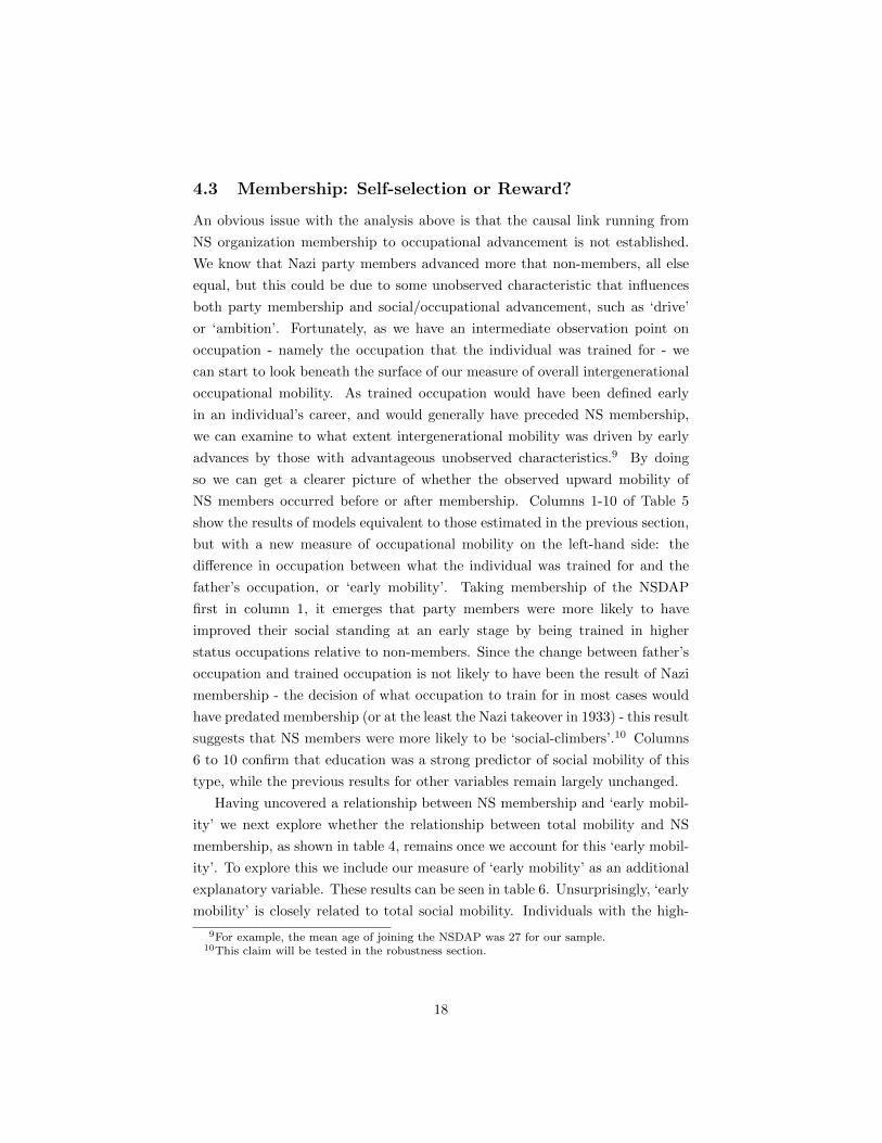
4.3 Membership: Self-selection or Reward?

An obvious issue with the analysis above is that the causal link running from

NS organization membership to occupational advancement is not established.

We know that Nazi party members advanced more that non-members, all else

equal, but this could be due to some unobserved characteristic that influences

both party membership and social/occupational advancement, such as ‘drive’

or ‘ambition’. Fortunately, as we have an intermediate observation point on

occupation - namely the occupation that the individual was trained for - we

can start to look beneath the surface of our measure of overall intergenerational

occupational mobility. As trained occupation would have been defined early

in an individual’s career, and would generally have preceded NS membership,

we can examine to what extent intergenerational mobility was driven by early

advances by those with advantageous unobserved characteristics.9 By doing

so we can get a clearer picture of whether the observed upward mobility of

NS members occurred before or after membership. Columns 1-10 of Table 5

show the results of models equivalent to those estimated in the previous section,

but with a new measure of occupational mobility on the left-hand side: the

difference in occupation between what the individual was trained for and the

father’s occupation, or ‘early mobility’. Taking membership of the NSDAP

first in column 1, it emerges that party members were more likely to have

improved their social standing at an early stage by being trained in higher

status occupations relative to non-members. Since the change between father’s

occupation and trained occupation is not likely to have been the result of Nazi

membership - the decision of what occupation to train for in most cases would

have predated membership (or at the least the Nazi takeover in 1933) - this result

suggests that NS members were more likely to be ‘social-climbers’.10 Columns

6 to 10 confirm that education was a strong predictor of social mobility of this

type, while the previous results for other variables remain largely unchanged.

Having uncovered a relationship between NS membership and ‘early mobil-

ity’ we next explore whether the relationship between total mobility and NS

membership, as shown in table 4, remains once we account for this ‘early mobil-

ity’. To explore this we include our measure of ‘early mobility’ as an additional

explanatory variable. These results can be seen in table 6. Unsurprisingly, ‘early

mobility’ is closely related to total social mobility. Individuals with the high-

9For example, the mean age of joining the NSDAP was 27 for our sample.10This claim will be tested in the robustness section.

18

est level of education appear to climb higher than those with lower education

levels, even after controlling for early movement up the social ladder. However

the most important results in the context of our analysis are those that related

to NS membership. The relationship between NS membership and total social

mobility, after controlling for an individual’s ‘early mobility’ is not robust. The

relatively strong and significant relationship apparent in table 4 becomes a small

and insignificant effect. We interpret this as evidence that NS organisations at-

tracted individuals who climbed the social ladder early on in their careers. We

find little evidence that the apparent relationship between NS membership and

social mobility is driven by party members being able to achieve occupational

status beyond that of their level of training. Put differently, we find that the

‘selection’ effect dominates the ‘reward’ effect.

4.4 Membership: Date of Joining

Another approach to examining the relationship between social advancement

and NS membership is to look at differences between different types of mem-

bers. One particular way that membership can be differentiated is by date of

joining. It is conceivable that those joining the party after the Nazi takeover

in 1933 had different motivations to those members who joined when the party

was still on the political fringe before 1930. The Nazi party itself was con-

cerned enough about opportunistic new members flooding the party to restrict

the admission of new members between June 1933 and 1937 (Unger, 1974). In-

deed within the party, a distinct hierarchy emerged after 1933, with the Alte

Kampfer, or the old guard, displaying resentment towards the Septemberlinge -

those that joined the party in the wake of the September 1930 electoral break-

through. The Marzveilchen, (March Violets) - those who joined the party after

the 1933 seizure of power - were viewed with particular contempt (Grunberger,

2013). To examine whether date of joining the party is related to social mobility,

we divide our NS memberships into three categories: those who joined before

1931, those who joined between 1931 and 1932 and those that joined from 1933

onward. We then run regressions for each of our three measures of occupational

mobility with the results shown in Table 7. Taking membership of the NSDAP

first (column 1), it is evident that both early and late joiners were more likely

to be in a higher status occupation than that of their fathers. However, if we

examine the equivalent coefficients in the regression which includes ‘early mobil-

ity’ as an explanatory variable, we find little evidence of a relationship between

19

Table 5: EARLY MOBILITY & NS MEMBERSHIP

VA

RIA

BL

ES

(1)

(2)

(3)

(4)

(5)

(6)

(7)

(8)

(9)

(10

)

NS

mem

bers

hip

NS

DA

P0.1

4**

0.1

8***

0.1

3**

0.1

6***

(2.3

4)

(2.9

2)

(2.2

1)

(2.7

5)

SS

0.2

5***

0.2

9***

0.2

4***

0.2

8***

(4.3

1)

(5.0

9)

(4.5

1)

(5.1

6)

SA

0.1

1***

0.1

5***

0.0

9**

0.1

2***

(2.6

1)

(3.6

8)

(2.0

9)

(3.1

0)

HJ

0.1

3***

0.1

5***

0.1

1***

0.1

3***

(5.5

0)

(6.2

2)

(4.8

7)

(5.5

1)

Fa

ther'

s o

ccupa

tio

n-0

.71*

**

-0.7

2*

**

-0.7

2*

**

-0.7

2*

**

-0.7

2*

**

-0.7

6*

**

-0.7

6*

**

-0.7

6*

**

-0.7

6*

**

-0.7

6*

**

(-4

9.1

4)

(-4

9.5

7)

(-5

0.1

6)

(-4

9.0

4)

(-4

9.6

4)

(-5

2.9

2)

(-5

3.1

3)

(-5

3.5

3)

(-5

2.8

4)

(-5

3.5

1)

Sch

oo

ling

lev

el

Hig

h0.7

2***

0.7

2***

0.7

1***

0.7

1***

0.7

0***

(8.7

1)

(8.5

5)

(8.7

4)

(8.5

7)

(8.3

3)

Med

ium

0.3

4***

0.3

4***

0.3

4***

0.3

3***

0.3

3***

(4.4

5)

(4.4

0)

(4.4

2)

(4.3

0)

(4.2

1)

Lo

w0.0

90.0

90.0

90.0

90.0

8(1

.17)

(1.1

6)

(1.1

6)

(1.1

4)

(1.0

9)

Unk

now

n0.2

7***

0.2

7***

0.2

6***

0.2

7***

0.2

6***

(3.3

8)

(3.3

5)

(3.3

3)

(3.3

4)

(3.2

7)

Relig

ion

Ro

man

Cat

holic

-0.0

3-0

.03

-0.0

3-0

.03

-0.0

2-0

.03

-0.0

2-0

.02

-0.0

2-0

.01

(-1

.43)

(-1

.26)

(-1

.41)

(-1

.36)

(-0

.77)

(-1

.14)

(-0

.97)

(-1

.14)

(-1

.09)

(-0

.55)

Co

ntr

ols

Yea

r o

r b

irth

YE

SY

ES

YE

SY

ES

YE

SY

ES

YE

SY

ES

YE

SY

ES

Age

at m

edic

al e

xam

inat

ion

YE

SY

ES

YE

SY

ES

YE

SY

ES

YE

SY

ES

YE

SY

ES

Urb

anis

atio

nY

ES

YE

SY

ES

YE

SY

ES

YE

SY

ES

YE

SY

ES

YE

SD

istr

ict fix

ed e

ffec

tsY

ES

YE

SY

ES

YE

SY

ES

YE

SY

ES

YE

SY

ES

YE

S

Co

nsta

nt-3

8.5

1*

**

-40

.29

***

-42

.65

***

-17

.17

*-1

8.6

2*

*-6

5.3

5*

**

-67

.02

***

-67

.82

***

-46

.93

***

-47

.66

***

(-4

.70)

(-4

.98)

(-5

.10)

(-1

.87)

(-1

.99)

(-6

.22)

(-6

.39)

(-6

.49)

(-4

.30)

(-4

.37)

Ob

serv

atio

ns9,9

94

9,9

94

9,9

94

9,9

94

9,9

94

9,9

94

9,9

94

9,9

94

9,9

94

9,9

94

R-s

qua

red

0.3

50.3

50.3

50.3

50.3

60.3

70.3

70.3

70.3

70.3

7C

lust

er r

ob

ust (k

reis

) t-

stat

istic

s in

par

enth

eses

, *

**

p<

0.0

1,

** p

<0

.05,

* p

<0.1

. A

ll re

fere

nce

cate

gories

are

as

in T

able

2.

20

Table 6: TOTAL MOBILITY & NS MEMBERSHIP INC. EARLY MOBILITY

VA

RIA

BL

ES

(1)

(2)

(3)

(4)

(5)

(6)

(7)

(8)

(9)

(10

)

NS

mem

bers

hip

NS

DA

P0.0

80.0

8*

0.0

80.0

8(1

.64)

(1.7

3)

(1.5

5)

(1.6

2)

SS

0.0

70.0

70.0

60.0

7(1

.51)

(1.5

8)

(1.4

1)

(1.4

6)

SA

0.0

20.0

20.0

10.0

2(0

.84)

(0.9

9)

(0.5

3)

(0.6

5)

HJ

-0.0

1-0

.00

-0.0

1-0

.01

(-0

.59)

(-0

.26)

(-0

.73)

(-0

.46)

Fa

ther'

s o

ccupa

tio

n-0

.25*

**

-0.2

5*

**

-0.2

5*

**

-0.2

5*

**

-0.2

5*

**

-0.2

7*

**

-0.2

7*

**

-0.2

7*

**

-0.2

7*

**

-0.2

7*

**

(-2

2.5

1)

(-2

2.3

9)

(-2

2.4

3)

(-2

2.4

5)

(-2

2.1

3)

(-2

2.0

0)

(-2

1.9

1)

(-2

1.9

7)

(-2

1.9

9)

(-2

1.7

0)

Ea

rly

Mo

bilit

y0.6

6***

0.6

6***

0.6

6***

0.6

6***

0.6

6***

0.6

5***

0.6

5***

0.6

5***

0.6

6***

0.6

5***

(54

.40

)(5

4.7

7)

(54

.76

)(5

4.6

5)

(54

.54

)(5

1.1

1)

(51

.52

)(5

1.5

4)

(51

.42

)(5

1.2

5)

Sch

oo

ling

lev

el

Hig

h0.1

2*

0.1

2*

0.1

2*

0.1

2*

0.1

2*

(1.7

5)

(1.7

4)

(1.7

5)

(1.7

6)

(1.7

3)

Med

ium

-0.0

1-0

.01

-0.0

1-0

.01

-0.0

1(-

0.2

9)

(-0

.27)

(-0

.29)

(-0

.27)

(-0

.28)

Lo

w-0

.09*

-0.0

8*

-0.0

9*

-0.0

8*

-0.0

8*

(-1

.86)

(-1

.84)

(-1

.86)

(-1

.85)

(-1

.85)

Unk

now

n-0

.04

-0.0

4-0

.04

-0.0

4-0

.04

(-0

.90)

(-0

.89)

(-0

.92)

(-0

.91)

(-0

.90)

Relig

ion

Ro

man

Cat

holic

-0.0

0-0

.00

-0.0

0-0

.00

-0.0

0-0

.00

-0.0

0-0

.00

-0.0

00.0

0(-

0.2

0)

(-0

.17)

(-0

.26)

(-0

.32)

(-0

.04)

(-0

.13)

(-0

.10)

(-0

.19)

(-0

.24)

(0.0

1)

Co

ntr

ols

Yea

r o

r b

irth

YE

SY

ES

YE

SY

ES

YE

SY

ES

YE

SY

ES

YE

SY

ES

Age

at m

edic

al e

xam

inat

ion

YE

SY

ES

YE

SY

ES

YE

SY

ES

YE

SY

ES

YE

SY

ES

Urb

anis

atio

nY

ES

YE

SY

ES

YE

SY

ES

YE

SY

ES

YE

SY

ES

YE

SD

istr

ict fix

ed e

ffec

tsY

ES

YE

SY

ES

YE

SY

ES

YE

SY

ES

YE

SY

ES

YE

S

Co

nsta

nt-2

4.7

4*

**

-25

.28

***

-25

.61

***

-26

.41

***

-26

.40

***

-30

.21

***

-30

.66

***

-30

.62

***

-32

.03

***

-32

.00

***

(-4

.48)

(-4

.54)

(-4

.57)

(-3

.99)

(-4

.00)

(-4

.29)

(-4

.33)

(-4

.34)

(-4

.10)

(-4

.14)

Ob

serv

atio

ns8,8

84

8,8

84

8,8

84

8,8

84

8,8

84

8,8

84

8,8

84

8,8

84

8,8

84

8,8

84

R-s

qua

red

0.6

90.6

90.6

90.6

90.6

90.7

00.7

00.7

00.7

00.7

0C

lust

er r

ob

ust (k

reis

) t-

stat

istic

s in

par

enth

eses

, *

**

p<

0.0

1,

** p

<0

.05,

* p

<0.1

. A

ll re

fere

nce

cate

gories

are

as

in T

able

2.

21

membership and mobility (column 6). This indicates that, even for members

that joined the party early on, social mobility predated membership and that

’socially mobile’ individuals self-selected into membership. For the SS and SA,

it would appear that the positive relationship between membership and social

mobility observed in tables 4 and 5 is driven mainly by those who joined the

part from 1933 onward.

5 Robustness

The previous section uncovered a link between party membership and occupa-

tional advancement and that this link was mainly driven by individuals who

demonstrated early mobility self-selecting into NS membership. However, there

are a number of checks that must be performed to test the robustness of these

findings. Firstly, there are likely to be non-linearities in the measure of social

mobility employed. To test the robustness of our result, we run a series of

different formulations of the dependent variable. Instead of defining the social

mobility variable as an integer number between -4 and 4, we re-code it as a

binary variable that equals one if there is a positive (negative) change in oc-

cupational status (i.e. change is equal to one (minus one)) and zero otherwise.

We also examine whether big changes in occupational status were associated

with NS memberships, as well as examining the likelihood of retaining the same

occupational status.11 Finally, we implement an ordered probit model, rank-

ing changes in occupational status from greatest fall to greatest increase. Our

conclusions, based on the original analysis, remain unaltered.12

In the analysis of the previous section the assumption is made that NS

membership did not influence the occupation than an individual was trained for.

To test this assumption we exclude individuals that, in all likelihood, would have

had their trained occupation determined after the Nazi seizure of power, namely

individuals that were under eighteen years of age in 1933.13 Reassuringly, the

results of the previous analysis are similar to those using this reduced sample

(appendix Table A1).

11“Big” changes were defined as movements greater than plus or minus 1.12Results reported in the appenix, tables A2-A7.13We also consider cut-offs of twenty-one and sixteen in 1933 (not reported).

22

Tab

le7:

SO

CIA

LM

OB

ILIT

Y&

DA

TE

OF

NS

ME

MB

ER

SH

IP

VA

RIA

BL

ES

(1)

(2)

(3)

(4)

(5)

(6)

(7)

(8)

(9)

(10)

(11)

(12)

(13)

(14)

(15)

NS

mem

bers

hip

NS

DA

P P

RE

1931

0.5

7***

0.5

9***

0.4

3***

0.4

5***

0.1

70.1

7(3

.98)

(4.1

9)

(2.9

8)

(3.1

9)

(1.1

5)

(1.1

8)

NS

DA

P 1

931-1

932

0.1

80.2

10.1

10.1

40.1

00.1

0(1

.38)

(1.5

7)

(0.7

1)

(0.9

1)

(0.9

8)

(1.0

2)

NS

DA

P P

OS

T 1

932

0.1

7***

0.1

9***

0.1

2*

0.1

5**

0.0

80.0

8(2

.88)

(3.2

3)

(1.7

1)

(2.0

7)

(1.3

4)

(1.3

8)

SS

PR

E 1

931

-0.0

4-0

.02

0.2

30.2

5*

-0.1

6-0

.15

(-0.2

1)

(-0.1

1)

(1.5

8)

(1.7

0)

(-1.3

7)

(-1.3

7)

SS

1931-1

932

0.1

70.2

0-0

.05

-0.0

30.1

80.1

8(1

.30)

(1.4

5)

(-0.5

1)

(-0.2

8)

(1.1

2)

(1.1

6)

SS

PO

ST

1932

0.2

7***

0.3

0***

0.3

1***

0.3

5***

0.0

60.0

6(3

.78)

(4.1

6)

(5.1

8)

(5.7

9)

(1.3

4)

(1.3

8)

SA

PR

E 1

931

-0.2

3-0

.21

0.0

80.1

1-0

.27*

-0.2

7*

(-1.3

4)

(-1.2

3)

(0.5

3)

(0.7

1)

(-1.7

4)

(-1.7

2)

SA

1931-1

932

0.0

10.0

30.0

30.0

5-0

.00

0.0

0(0

.11)

(0.2

8)

(0.2

7)

(0.5

3)

(-0.0

4)

(0.0

1)

SA

PO

ST

1932

0.0

9**

0.1

1***

0.0

8**

0.1

2***

0.0

30.0

4(2

.28)

(2.9

7)

(2.0

0)

(2.9

5)

(1.3

4)

(1.4

6)

HJ

PR

E 1

931

-0.0

4-0

.02

-0.0

10.0

0-0

.00

0.0

0(-

0.3

7)

(-0.2

1)

(-0.1

4)

(0.0

4)

(-0.0

5)

(0.0

0)

HJ

1931-1

932

-0.0

8-0

.06

-0.0

8-0

.06

-0.0

8**

-0.0

8*

(-1.5

0)

(-1.1

6)

(-1.2

8)

(-0.9

5)

(-2.0

0)

(-1.8

9)

HJ

PO

ST

1932

0.0

7***

0.0

9***

0.1

3***

0.1

5***

-0.0

1-0

.00

(3.5

4)

(4.2

6)

(5.4

8)

(6.1

5)

(-0.3

7)

(-0.0

5)

Fath

er'

s occ

upati

on

-0.7

7***

-0.7

6***

-0.7

7***

-0.7

7***

-0.7

7***

-0.7

6***

-0.7

6***

-0.7

6***

-0.7

6***

-0.7

6***

-0.2

7***

-0.2

7***

-0.2

7***

-0.2

7***

-0.2

7***

(-52.2

6)

(-52.3

9)

(-52.9

1)

(-52.5

9)

(-52.7

5)

(-52.9

0)

(-53.2

5)

(-53.4

8)

(-53.0

5)

(-53.7

7)

(-21.8

5)

(-21.9

1)

(-21.9

8)

(-22.1

3)

(-21.7

2)

Earl

y M

obilit

y0.6

5***

0.6

5***

0.6

5***

0.6

5***

0.6

5***

(50.9

3)

(51.4

8)

(51.5

1)

(51.5

5)

(51.1

4)

Sch

ooling level

Hig

h0.8

0***

0.8

0***

0.8

0***

0.8

0***

0.7

9***

0.7

2***

0.7

1***

0.7

1***

0.7

2***

0.7

0***

0.1

2*

0.1

2*

0.1

2*

0.1

2*

0.1

2*

(12.1

9)

(12.0

4)

(12.1

4)

(11.9

9)

(11.7

0)

(8.7

2)

(8.4

7)

(8.7

3)

(8.6

4)

(8.3

2)

(1.7

4)

(1.7

8)

(1.7

3)

(1.7

8)

(1.7

5)

Med

ium

0.2

9***

0.2

9***

0.2

9***

0.2

9***

0.2

8***

0.3

4***

0.3

4***

0.3

4***

0.3

4***

0.3

3***

-0.0

2-0

.01

-0.0

1-0

.01

-0.0

1(5

.18)

(5.1

5)

(5.2

2)

(5.1

5)

(4.9

9)

(4.4

3)

(4.3

5)

(4.4

3)

(4.3

3)

(4.1

7)

(-0.3

0)

(-0.2

6)

(-0.2

6)

(-0.2

5)

(-0.2

5)

Low

0.0

80.0

90.0

90.0

90.0

80.0

90.0

90.0

90.0

90.0

9-0

.09*

-0.0

8*

-0.0

8*

-0.0

8*

-0.0

8*

(1.5

4)

(1.5

4)

(1.5

6)

(1.5

6)

(1.5

0)

(1.1

7)

(1.1

4)

(1.1

7)

(1.1

9)

(1.1

2)

(-1.8

7)

(-1.8

2)

(-1.8

5)

(-1.8

2)

(-1.8

1)

Unk

now

n0.2

7***

0.2

7***

0.2

6***

0.2

7***

0.2

6***

0.2

7***

0.2

7***

0.2

6***

0.2

7***

0.2

6***

-0.0

4-0

.04

-0.0

4-0

.04

-0.0

4(4

.55)

(4.5

0)

(4.4

5)

(4.4

7)

(4.3

2)

(3.3

8)

(3.3

2)

(3.3

4)

(3.3

5)

(3.2

5)

(-0.9

0)

(-0.8

8)

(-0.9

5)

(-0.9

0)

(-0.9

1)

Religio

n

Rom

an C

atho

lic-0

.01

-0.0

1-0

.01

-0.0

1-0

.00

-0.0

3-0

.02

-0.0

3-0

.02

-0.0

1-0

.00

-0.0

0-0

.00

-0.0

00.0

0(-

0.6

5)

(-0.5

0)

(-0.7

0)

(-0.6

6)

(-0.1

6)

(-1.1

5)

(-1.0

1)

(-1.1

6)

(-1.1

1)

(-0.6

4)

(-0.1

2)

(-0.0

5)

(-0.1

9)

(-0.2

4)

(0.0

7)

Contr

ols

Yea

r or

birth

YE

SY

ES

YE

SY

ES

YE

SY

ES

YE

SY

ES

YE

SY

ES

YE

SY

ES

YE

SY

ES

YE

SA

ge a

t m

edic

al e

xam

inat

ion

YE

SY

ES

YE

SY

ES

YE

SY

ES

YE

SY

ES

YE

SY

ES

YE

SY

ES

YE

SY

ES

YE

SU

rban

isat

ion

YE

SY

ES

YE

SY

ES

YE

SY

ES

YE

SY

ES

YE

SY

ES

YE

SY

ES

YE

SY

ES

YE

SD

istr

ict fix

ed e

ffec

tsY

ES

YE

SY

ES

YE

SY

ES

YE

SY

ES

YE

SY

ES

YE

SY

ES

YE

SY

ES

YE

SY

ES

Obse

rvat

ions

10,0

00

10,0

00

10,0

00

10,0

00

10,0

00

9,9

94

9,9

94

9,9

94

9,9

94

9,9

94

8,8

84

8,8

84

8,8

84

8,8

84

8,8

84

R-s

qua

red

0.4

00.4

00.4

00.4

00.4

10.3

70.3

70.3

70.3

70.3

80.7

00.7

00.7

00.7

00.7

0C

lust

er r

obus

t (k

reis

) t-

stat

istic

s in

par

enth

eses

, *** p

<0.0

1, ** p

<0.0

5, * p

<0.1

. A

ll re

fere

nce

cate

gories

are

as

in T

able

2. A

ll m

odel

s in

clud

e a

cons

tant

.

Tota

l S

oci

al M

obilit

yE

arl

y M

obilit

yT

ota

l S

oci

al M

obilit

y (

inc.

Earl

y M

obilit

y)

23

6 Conclusion

Do members of political organizations receive economic benefits? Or are more

‘driven’ or ‘high ability’ types more likely to join? Our analysis suggests that,

in the case of the rank and file of NS organisations, the relationship between

between social advancement and political connections is driven primarily by the

latter. In the first part of the paper we examine the determinants of Nazi mem-

bership and add a unique perspective to this substantial literature. We find

that higher-educated individuals and those from higher socioeconomic back-

grounds were more likely to be members of not just the NSDAP, but all NS

organisations. We then undertake something more novel, exploring the rela-

tionship between membership of NS organisations and socioeconomic mobility.

We find a positive relationship between NS membership and intergenerational

occupational advancement. Indeed we find that this relationship is stronger for

the more ‘elite’ NS organisations, the NSDAP and the SS. However, we also un-

cover that NS members were more likely to have achieved social advancement at

an early stage, suggesting that these individuals self-selected into membership.

Although we cannot say whether members benefitted in other ways, such as

through direct financial rewards or non-monetary benefits, our findings suggest

that the observed positive relationship between social mobility and NS mem-

bership was driven mainly by unobserved charateristics. We find little evidence

in our analysis of a direct ‘reward’ effect for members once we control for this

‘early mobility’. Additionally we find that both early and late NSDAP joiners

demonstrated higher ‘early mobility’. Even among early joiners of the party our

analysis uncovers little evidence of direct patronage.

References

Acemoglu, D., S. Johnson, A. Kermani, J. Kwak, and T. Mitton (2013). The

value of connections in turbulent times: Evidence from the united states.

NBER Working Paper 19701.

Appleton, S., J. Knight, L. Song, and Q. Xia (2009). The economics of commu-

nist party membership: The curious case of rising numbers and wage premium

during china’s transition. The Journal of Development Studies 45 (2), 256–

275.

Armstrong, W. (1972). The use of information about occupation. In E. Wrigley

24

(Ed.), Nineteenth-Century Society, Anglica Germanica, pp. 191–311. Cam-

bridge University Press.

Ault, B. (2002). Joining the nazi party before 1930. Social Science His-

tory 26 (02), 273–310.

Bendix, R. (1952, Jun.). Social stratification and political power. The American

Political Science Review 46 (2), 357–375.

Bodenhorn, H., T. W. Guinnane, and T. A. Mroz (2015). Sample-selection

biases and the ”industrialization puzzle”. Technical report, National Bureau

of Economic Research.

Brustein, W. (1998). The Logic of Evil: The Social Origins of the Nazi Party,

1925-1933. Yale University Press. ID: 230; 95047263.

Childers, T. (1976). The social bases of the national socialist vote. Journal of

Contemporary History 11 (4, Special Issue: Theories of Fascism), pp. 17–42.

ID: 88.

Childers, T. (1983). The Nazi voter: the social foundations of fascism in Ger-

many, 1919-1933. Chapel Hill: University of North Carolina Press. ID: 91;

83005924.

Claessens, S., E. Feijen, and L. Laeven (2008). Political connections and pref-

erential access to finance: The role of campaign contributions. Journal of

Financial Economics 88 (3), 554–580.

Faccio, M. (2006). Politically connected firms. The American Economic Re-

view 96 (1), 369–386.

Falter, J. (1991). Hitlers Wahler. C.H. Besck.

Falter, J. (2000). The nsdap: A ’people’s protest party’. In N. Gregor (Ed.),

Nazism, Oxford readers, pp. 92–94. Oxford University Press.

Ferguson, T. and H.-J. Voth (2008). Betting on hitler: the value of political

connections in nazi germany. The Quarterly Journal of Economics, 101–137.

Fisman, R. (2001). Estimating the value of political connections. The American

Economic Review 91 (4), 1095–1102.

25

Gerber, T. P. (2000). Membership benefits or selection effects? why former

communist party members do better in post-soviet russia. Social science

research 29 (1), 25–50.

Grunberger, R. (2013). A social history of the Third Reich. Hachette UK.

Hamilton, R. F. (1982). Who voted for Hitler? Princeton University Press.

Kaplan, M. A. (1998). Between dignity and despair: Jewish life in Nazi Ger-

many. Oxford University Press.

Kater, M. (1985). The Nazi Party: A Social Profile of Members and Leaders

1919-1945. Basil Blackwell.

Kater, M. H. (1983). The Nazi party: A social profile of members and leaders,

1919-1945. Cambridge, Mass.: Harvard University Press.

King, G., O. Rosen, M. Tanner, and A. F. Wagner (2008). Ordinary economic

voting behavior in the extraordinary election of adolf hitler. The Journal of

Economic History 68 (04), 951–996.

Lepage, J. (2008). Hitler Youth, 1922-1945: An Illustrated History. McFarland,

Incorporated Publishers.

Li, H., P. W. Liu, J. Zhang, and N. Ma (2007). Economic returns to commu-

nist party membership: Evidence from urban chinese twins. The Economic

Journal 117 (523), 1504–1520.

Li, H., L. Meng, X. Shi, and B. Wu (2012). Does having a cadre parent pay?

evidence from the first job offers of chinese college graduates. Journal of

Development Economics 99 (2), 513 – 520.

Lipset, S. and R. Bendix (1991). Social Mobility in Industrial Society. A pub-

lication of the Institute of Industrial Relations, University of California. Uni-

versity of California Press.

Lipset, S. M. (1960). Political man: The social bases of politics. Seymour Martin

Lipset.

Long, J. and J. Ferrie (2013). Intergenerational occupational mobility in great

britain and the united states since 1850. The American Economic Re-

view 103 (4), 1109–1137.

26

Madden, P. (1987). The social class origins of nazi party members as determined

by occupations, 1919-1933. Social Science Quarterly , 263–280.

Mitchell, B. (1998). International Historical Statistics: Europe 1750-1993. In-

ternational Historical Statistics. Palgrave Macmillan UK.

MPIDR, C. (2011). Mpidr (max planck institute for demographic research) and

cgg (chair for geodesy and geoinformatics, population history gis collection

(partly based on bundesamt fur kartographie und geodasie 2011) rostock.

Muhlberger, D. (1991). Hitler’s Followers: Studies in the Sociology of the Nazi

Movement. Routledge. 90008455.

Parrish, T. and S. Marshall (1978). The Simon and Schuster encyclopedia of

World War II. Simon and Schuster.

Paterson, L. and C. Iannelli (2006). Religion, social mobility and education in

scotland. The British journal of sociology 57 (3), 353–377.

Rass, C. (2001). Menschenmaterial: Sozialprofil, machtstrukturen und hand-

lungsmuster einer infanteriedivision der wehrmacht im zweiten weltkrieg.

Rass, C. (2003). Menschenmaterial: Deutsche Soldaten an der Ostfront; In-

nenansichten einer Infanteriedivision 1939-1945, Volume 17. Schoningh.

Satyanath, S., N. Voigtlaender, and H.-J. Voth (2013). Bowling for fascism:

social capital and the rise of the nazi party. Technical report, National Bureau

of Economic Research.

Spenkuch, J. and P. Tillmann (2016). Special interests at the ballot box? religion

and the electoral success of the nazis. Technical report, Working Paper.

Stachura, P. (2014a). The Nazi Machtergreifung (RLE Nazi Germany & Holo-

caust). Routledge Library Editions: Nazi Germany and the Holocaust. Taylor

& Francis.

Stachura, P. D. (2014b). The Shaping of the Nazi State (RLE Nazi Germany

and Holocaust). Routledge.

Unger, A. L. (1974). The totalitarian party: party and people in Nazi Germany

and Soviet Russia. Cambridge University Press.

Weber, M. (2005). The Protestant Ethic and the Spirit of Capitalism. Routledge

Classics. Taylor & Francis.

27

Appendix

VA

RIA

BL

ES

(1)

(2)

(3)

(4)

(5)

(6)

(7)

(8)

(9)

(10

)(1

1)

(12

)(1

3)

(14

)(1

5)

NS

mem

bers

hip

NS

DA

P P

RE

19

31

0.5

2*

**

0.5

3*

**

0.2

90

.31

*0

.20

0.2

0(3

.28

)(3

.44

)(1

.62

)(1

.75

)(1

.15

)(1

.17

)N

SD

AP

19

31

-19

32

0.2

00

.23

0.1

20

.15

0.1

30

.14

(1.4

3)

(1.6

3)

(0.7

5)

(0.9

1)

(1.3

4)

(1.4

1)

NS

DA

P P

OS

T 1

93

30

.12

*0

.14

*0

.11

0.1

3*

0.0

70

.08

(1.6

6)

(1.9

5)

(1.4

6)

(1.7

3)

(1.0

6)

(1.1

3)

SS

PR

E 1

93

00

.04

0.0

60

.26

0.2

8-0

.11

-0.1

1(0

.18

)(0

.24

)(1

.18

)(1

.26

)(-

0.7

4)

(-0

.76

)S

S 1

93

0-1

93

30

.21

0.2

2-0

.06

-0.0

40

.19

0.2

0(1

.32

)(1

.42

)(-

0.6

0)

(-0

.41

)(1

.10

)(1

.12

)S

S P

OS

T 1

93

30

.29

**

*0

.32

**

*0

.31

**

*0

.33

**

*0

.08

0.0

9(3

.18

)(3

.34

)(3

.10

)(3

.30

)(1

.10

)(1

.18

)S

A P

RE

19

30

-0.3

4-0

.32

0.0

30

.05

-0.3

2*

-0.3

2*

(-1

.62

)(-

1.5

4)

(0.1

8)

(0.2

7)

(-1

.69

)(-

1.6

6)

SA

19

30

-19

33

0.0

10

.03

0.0

60

.08

-0.0

5-0

.05

(0.1

0)

(0.2

0)

(0.6

4)

(0.8

2)

(-0

.59

)(-

0.5

3)

SA

PO

ST

19

33

0.1

2*

**

0.1

4*

**

0.1

2*

*0

.14

**

0.0

40

.04

(2.6

8)

(3.0

6)

(2.1

8)

(2.4

8)

(1.0

6)

(1.2

4)

HJ

PR

E 1

93

00

.10

0.1

3-0

.00

0.0

30

.08

0.0

9(0

.51

)(0

.62

)(-

0.0

0)

(0.0

8)

(0.8

1)

(0.8

6)

HJ

19

30

-19

33

-0.4

0*

-0.3

8*

0.0

80

.11

-0.4

6*

*-0

.45

**

(-1

.89

)(-

1.7

5)

(0.3

5)

(0.4

4)

(-2

.12

)(-

2.0

8)

HJ

PO

ST

19

33

-0.0

7-0

.04

-0.0

10

.02

-0.0

2-0

.02

(-0

.43

)(-

0.2

5)

(-0

.06

)(0

.13

)(-

0.3

4)

(-0

.24

)F

ath

er'

s o

ccu

pa

tio

n-0

.71

**

*-0

.71

**

*-0

.71

**

*-0

.71

**

*-0

.71

**

*-0

.71

**

*-0

.71

**

*-0

.71

**

*-0

.71

**

*-0

.71

**

*-0

.28

**

*-0

.28

**

*-0

.28

**

*-0

.28

**

*-0

.28

**

*(-

35

.03

)(-

35

.15

)(-

35

.68

)(-

35

.19

)(-

36

.07

)(-

32

.22

)(-

32

.37

)(-

32

.78

)(-

32

.25

)(-

33

.10

)(-

14

.12

)(-

14

.08

)(-

14

.08

)(-

14

.19

)(-

14

.17

)E

arl

y M

ob

ilit

y0

.61

**

*0

.61

**

*0

.61

**

*0

.61

**

*0

.61

**

*(3

4.6

1)

(34

.70

)(3

5.0

2)

(34

.87

)(3

4.4

1)

Sch

oo

lin

g l

ev

el

Hig

h0

.87

**

*0

.87

**

*0

.86

**

*0

.88

**

*0

.84

**

*1

.09

**

*1

.08

**

*1

.08

**

*1

.10

**

*1

.05

**

*0

.01

0.0

20

.01

0.0

20

.02

(5.7

9)

(5.7

8)

(5.8

7)

(5.9

2)

(5.6

8)

(6.9

7)

(6.8

1)

(7.0

7)

(7.0

6)

(6.7

2)

(0.0

7)

(0.1

2)

(0.0

8)

(0.1

1)

(0.0

8)

Med

ium

0.3

5*

*0

.35

**

0.3

5*

*0

.36

**

0.3

4*

*0

.55

**

*0

.55

**

*0

.55

**

*0

.56

**

*0

.53

**

*-0

.09

-0.0

9-0

.09

-0.0

9-0

.09

(2.4

8)

(2.5

1)

(2.5

2)

(2.5

5)

(2.4

0)

(3.2

2)

(3.1

7)

(3.2

1)

(3.2

5)

(3.0

7)

(-0

.54

)(-

0.4

9)

(-0

.50

)(-

0.5

0)

(-0

.49

)L

ow

0.1

00

.11

0.1

10

.11

0.1

00

.22

0.2

20

.22

0.2

20

.20

-0.2

0-0

.19

-0.2

0-0

.20

-0.1

9(0

.81

)(0

.84

)(0

.82

)(0

.86

)(0

.76

)(1

.31

)(1

.28

)(1

.30

)(1

.34

)(1

.21

)(-

1.2

5)

(-1

.19

)(-

1.2

1)

(-1

.21

)(-

1.1

8)

Unk

now

n0

.29

**

0.2

9*

*0

.28

**

0.2

9*

*0

.27

**

0.3

7*

*0

.37

**

0.3

6*

*0

.38

**

0.3

5*

*-0

.12

-0.1

1-0

.12

-0.1

1-0

.12

(2.4

8)

(2.5

1)

(2.4

2)

(2.5

6)

(2.3

6)

(2.1

5)

(2.1

0)

(2.1

1)

(2.1

7)

(2.0

1)

(-0

.78

)(-

0.7

4)

(-0

.78

)(-

0.7

3)

(-0

.74

)R

eli

gio

n

Ro

man

Cat

holic

-0.0

2-0

.01

-0.0

2-0

.02

-0.0

1-0

.03

-0.0

3-0

.03

-0.0

3-0

.02

-0.0

0-0

.00

-0.0

1-0

.01

0.0

0(-

0.5

7)

(-0

.38

)(-

0.6

4)

(-0

.70

)(-

0.2

0)

(-0

.96

)(-

0.8

3)

(-0

.95

)(-

1.0

3)

(-0

.61

)(-

0.1

3)

(-0

.06

)(-

0.2

5)

(-0

.27

)(0

.03

)

Co

ntr

ols

Yea

r o

r b

irth

YE

SY

ES

YE

SY

ES

YE

SY

ES

YE

SY

ES

YE

SY

ES

YE

SY

ES

YE

SY

ES

YE

SA

ge a

t m

edic

al e

xam

inat

ion

YE

SY

ES

YE

SY

ES

YE

SY

ES

YE

SY

ES

YE

SY

ES

YE

SY

ES

YE

SY

ES

YE

SU

rban

isat

ion

YE

SY

ES

YE

SY

ES

YE

SY

ES

YE

SY

ES

YE

SY

ES

YE

SY

ES

YE

SY

ES

YE

SD

istr

ict

fixed

eff

ects

YE

SY

ES

YE

SY

ES

YE

SY

ES

YE

SY

ES

YE

SY

ES

YE

SY

ES

YE

SY

ES

YE

S

Ob

serv

atio

ns4

,18

64

,18

64

,18

64

,18

64

,18

64

,34

44

,34

44

,34

44

,34

44

,34

43

,77

53

,77

53

,77

53

,77

53

,77

5R

-sq

uare

d0

.41

0.4

10

.41

0.4

00

.41

0.3

90

.39

0.3

90

.39

0.3

90

.65

0.6

50

.65

0.6

50

.65

Clu

ster

ro

bus

t (k

reis

) t-

stat

istic

s in

par

enth

eses

, *

**

p<

0.0

1,

**

p<

0.0

5,

* p

<0

.1.

All

refe

renc

e ca

tego

ries

are

as

in T

able

2.

All

mo

del

s in

clud

e a

cons

tant

.

To

tal

So

cia

l M

ob

ilit

yE

arl

y M

ob

ilit

yT

ota

l S

oci

al

Mo

bil

ity

(in

c. E

arl

y M

ob

ilit

y)

Tab

le A

1: S

OC

IAL

MO

BIL

ITY

AN

D D

AT

E O

F N

S M

EM

BE

RS

HIP

- O

NL

Y I

ND

IVID

UA

LS

AG

ED

18

AN

D O

VE

R I

N 1

93

3

28

VARIABLES (1) (2) (3) (4) (5) (6) (7) (8)

NS membership

NSDAP 0.34* 0.12(1.68) (0.46)

SS -0.07 -0.51*(-0.31) (-1.77)

SA 0.11 -0.08(0.93) (-0.54)

HJ 0.35*** 0.22**(4.53) (2.35)

Father's occupation -1.88*** -1.00*** -1.88*** -1.00*** -1.88*** -1.00*** -1.89*** -1.01***(-34.61) (-14.62) (-34.59) (-14.55) (-34.59) (-14.58) (-34.70) (-14.72)

Early Mobility 1.83*** 1.83*** 1.83*** 1.82***(31.83) (31.89) (31.85) (31.71)

Schooling level

High 1.79*** 0.33 1.80*** 0.34 1.80*** 0.33 1.79*** 0.33(6.62) (0.94) (6.67) (0.97) (6.64) (0.96) (6.60) (0.95)

Medium 0.60*** 0.07 0.61*** 0.07 0.61*** 0.07 0.58** 0.06(2.64) (0.25) (2.66) (0.25) (2.65) (0.26) (2.53) (0.21)

Low 0.28 -0.01 0.28 -0.01 0.28 -0.01 0.27 -0.02(1.30) (-0.05) (1.31) (-0.05) (1.30) (-0.05) (1.25) (-0.06)

Unknown 0.57** 0.06 0.57** 0.06 0.57** 0.06 0.57** 0.06(2.52) (0.20) (2.51) (0.19) (2.48) (0.21) (2.49) (0.21)

Religion

Roman Catholic -0.01 0.01 -0.01 -0.00 -0.01 0.00 0.00 0.01(-0.08) (0.08) (-0.14) (-0.02) (-0.10) (0.05) (0.04) (0.15)

Controls

Year or birth YES YES YES YES YES YES YES YESAge at medical examination YES YES YES YES YES YES YES YESUrbanisation YES YES YES YES YES YES YES YESDistrict fixed effects YES YES YES YES YES YES YES YES

Observations 9,430 8,360 9,430 8,360 9,430 8,360 9,430 8,360z-statistics in parentheses, *** p<0.01, ** p<0.05, * p<0.1.

Fixed effects logit model. All reference categories are as in Table 2.

TABLE A2: POSITIVE (+1) SOCIAL MOBILITY AND NS MEMBERSHIP INCLUDING EARLY MOBILITY

29

VARIABLES (1) (2) (3) (4) (5) (6) (7) (8)

NS membership

NSDAP -0.26 -0.14(-1.23) (-0.54)

SS -0.30 -0.15(-1.34) (-0.59)

SA 0.01 0.06(0.13) (0.47)

HJ -0.02 0.10(-0.27) (1.03)

Father's occupation 1.13*** 0.42*** 1.13*** 0.43*** 1.13*** 0.42*** 1.13*** 0.42***(28.35) (8.28) (28.35) (8.28) (28.32) (8.23) (28.32) (8.15)

Early Mobility -1.33*** -1.33*** -1.33*** -1.33***(-28.97) (-28.94) (-28.98) (-28.99)

Schooling level

High -1.04*** 0.03 -1.04*** 0.03 -1.04*** 0.03 -1.04*** 0.03(-4.24) (0.11) (-4.26) (0.11) (-4.28) (0.09) (-4.27) (0.08)

Medium -0.54** -0.03 -0.54*** -0.04 -0.55*** -0.04 -0.54*** -0.04(-2.56) (-0.13) (-2.59) (-0.14) (-2.59) (-0.14) (-2.58) (-0.16)

Low -0.28 -0.02 -0.28 -0.02 -0.28 -0.03 -0.28 -0.03(-1.42) (-0.09) (-1.44) (-0.10) (-1.44) (-0.10) (-1.43) (-0.10)

Unknown -0.49** 0.01 -0.49** 0.01 -0.49** 0.00 -0.49** 0.01(-2.32) (0.03) (-2.33) (0.03) (-2.33) (0.02) (-2.33) (0.03)

Religion

Roman Catholic 0.06 0.05 0.05 0.05 0.06 0.06 0.06 0.06(0.83) (0.64) (0.77) (0.62) (0.87) (0.67) (0.85) (0.70)

Controls

Year or birth YES YES YES YES YES YES YES YESAge at medical examination YES YES YES YES YES YES YES YESUrbanisation YES YES YES YES YES YES YES YESDistrict fixed effects YES YES YES YES YES YES YES YES

Observations 9,446 8,364 9,446 8,364 9,446 8,364 9,446 8,364z-statistics in parentheses, *** p<0.01, ** p<0.05, * p<0.1.

Fixed effects logit model. All reference categories are as in Table 2.

TABLE A3: NEGATIVE (-1) SOCIAL MOBILITY AND NS MEMBERSHIP INCLUDING EARLY MOBILITY

30

VARIABLES (1) (2) (3) (4) (5) (6) (7) (8)

NS membership

NSDAP -0.03 -0.04(-0.19) (-0.23)

SS 0.13 0.14(0.78) (0.79)

SA -0.02 0.02(-0.27) (0.22)

HJ -0.21*** -0.22***(-3.45) (-3.38)

Father's occupation 0.08*** 0.17*** 0.08*** 0.17*** 0.08*** 0.17*** 0.09*** 0.18***(2.84) (4.31) (2.82) (4.27) (2.84) (4.29) (2.98) (4.53)

Early Mobility 0.04 0.04 0.04 0.05(1.40) (1.36) (1.39) (1.58)

Schooling level

High -0.52*** -0.51** -0.52*** -0.51** -0.52*** -0.51** -0.50** -0.51**(-2.58) (-2.33) (-2.60) (-2.34) (-2.58) (-2.34) (-2.52) (-2.30)

Medium -0.03 0.01 -0.03 0.01 -0.03 0.01 -0.01 0.02(-0.16) (0.04) (-0.16) (0.04) (-0.15) (0.04) (-0.07) (0.11)

Low 0.02 0.08 0.02 0.08 0.02 0.08 0.02 0.08(0.12) (0.46) (0.12) (0.46) (0.12) (0.46) (0.14) (0.48)

Unknown -0.01 0.03 -0.01 0.03 -0.01 0.03 -0.01 0.03(-0.09) (0.17) (-0.08) (0.18) (-0.08) (0.17) (-0.08) (0.17)

Religion

Roman Catholic -0.01 0.01 -0.01 0.01 -0.01 0.01 -0.02 0.00(-0.16) (0.18) (-0.11) (0.24) (-0.17) (0.19) (-0.31) (0.05)

Controls

Year or birth YES YES YES YES YES YES YES YESAge at medical examination YES YES YES YES YES YES YES YESUrbanisation YES YES YES YES YES YES YES YESDistrict fixed effects YES YES YES YES YES YES YES YES

Observations 9,542 8,471 9,542 8,471 9,542 8,471 9,542 8,471z-statistics in parentheses, *** p<0.01, ** p<0.05, * p<0.1.

Fixed effects logit model. All reference categories are as in Table 2.

TABLE A4: NO (0) SOCIAL MOBILITY AND NS MEMBERSHIP INCLUDING EARLY MOBILITY

31

VARIABLES (1) (2) (3) (4) (5) (6) (7) (8)

NS membership

NSDAP 0.97*** 0.60(2.66) (1.19)

SS 1.07*** 0.40(2.81) (0.73)

SA 0.39 0.31(1.45) (0.86)

HJ -0.03 -0.44(-0.12) (-1.53)

Father's occupation -2.88*** -1.75*** -2.87*** -1.73*** -2.88*** -1.75*** -2.87*** -1.72***(-20.36) (-8.20) (-20.29) (-8.16) (-20.34) (-8.19) (-20.31) (-8.11)

Early Mobility 2.71*** 2.72*** 2.72*** 2.73***(16.28) (16.31) (16.33) (16.38)

Schooling level

High 3.79*** 1.68** 3.71*** 1.59** 3.76*** 1.60** 3.78*** 1.59**(6.36) (2.09) (6.24) (1.97) (6.31) (1.99) (6.34) (1.99)

Medium 1.01* -0.15 1.01* -0.18 1.01* -0.18 1.03* -0.22(1.80) (-0.21) (1.81) (-0.26) (1.80) (-0.26) (1.83) (-0.32)

Low 0.02 -0.62 0.01 -0.64 0.02 -0.65 0.03 -0.67(0.04) (-0.94) (0.03) (-0.97) (0.04) (-0.98) (0.05) (-1.01)

Unknown 0.77 -0.23 0.73 -0.28 0.73 -0.29 0.75 -0.31(1.38) (-0.33) (1.31) (-0.40) (1.31) (-0.40) (1.33) (-0.44)

Religion

Roman Catholic -0.12 -0.13 -0.11 -0.12 -0.12 -0.12 -0.13 -0.15(-0.71) (-0.57) (-0.62) (-0.55) (-0.70) (-0.56) (-0.76) (-0.69)

Controls

Year or birth YES YES YES YES YES YES YES YESAge at medical examination YES YES YES YES YES YES YES YESUrbanisation YES YES YES YES YES YES YES YESDistrict fixed effects YES YES YES YES YES YES YES YES

Observations 8,751 7,678 8,751 7,678 8,751 7,678 8,751 7,678z-statistics in parentheses, *** p<0.01, ** p<0.05, * p<0.1.

Fixed effects logit model. All reference categories are as in Table 2.

TABLE A5: "BIG" (> +1) POSITIVE SOCIAL MOBILITY AND NS MEMBERSHIP INCLUDING EARLY MOBILITY

32

VARIABLES (1) (2) (3) (4) (5) (6) (7) (8)

NS membership

NSDAP -0.47 -0.22(-1.13) (-0.42)

SS -1.28** -1.20*(-2.32) (-1.86)

SA -0.18 -0.23(-0.85) (-0.85)

HJ -0.08 -0.01(-0.60) (-0.03)

Father's occupation 1.93*** 0.94*** 1.94*** 0.96*** 1.93*** 0.94*** 1.93*** 0.94***(25.57) (8.87) (25.59) (8.97) (25.57) (8.86) (25.54) (8.82)

Early Mobility -2.22*** -2.22*** -2.22*** -2.22***(-22.11) (-22.08) (-22.11) (-22.11)

Schooling level

High -1.70*** -0.10 -1.69*** -0.10 -1.69*** -0.07 -1.70*** -0.10(-3.77) (-0.16) (-3.75) (-0.15) (-3.75) (-0.10) (-3.79) (-0.15)

Medium -0.78* 0.40 -0.78** 0.38 -0.78* 0.41 -0.78* 0.39(-1.95) (0.67) (-1.97) (0.64) (-1.96) (0.68) (-1.96) (0.66)

Low -0.05 0.95* -0.05 0.96* -0.05 0.95* -0.05 0.95*(-0.14) (1.70) (-0.12) (1.72) (-0.14) (1.71) (-0.14) (1.69)

Unknown -0.96** 0.40 -0.96** 0.42 -0.96** 0.41 -0.97** 0.40(-2.41) (0.66) (-2.41) (0.71) (-2.39) (0.69) (-2.42) (0.67)

Religion

Roman Catholic 0.05 -0.06 0.03 -0.09 0.06 -0.05 0.05 -0.05(0.39) (-0.33) (0.24) (-0.49) (0.43) (-0.31) (0.41) (-0.30)

Controls

Year or birth YES YES YES YES YES YES YES YESAge at medical examination YES YES YES YES YES YES YES YESUrbanisation YES YES YES YES YES YES YES YESDistrict fixed effects YES YES YES YES YES YES YES YES

Observations 8,802 7,776 8,802 7,776 8,802 7,776 8,802 7,776z-statistics in parentheses, *** p<0.01, ** p<0.05, * p<0.1.

Fixed effects logit model. All reference categories are as in Table 2.

TABLE A6: "BIG" (<-1) NEGATIVE SOCIAL MOBILITY AND NS MEMBERSHIP INCLUDING EARLY MOBILITY

33

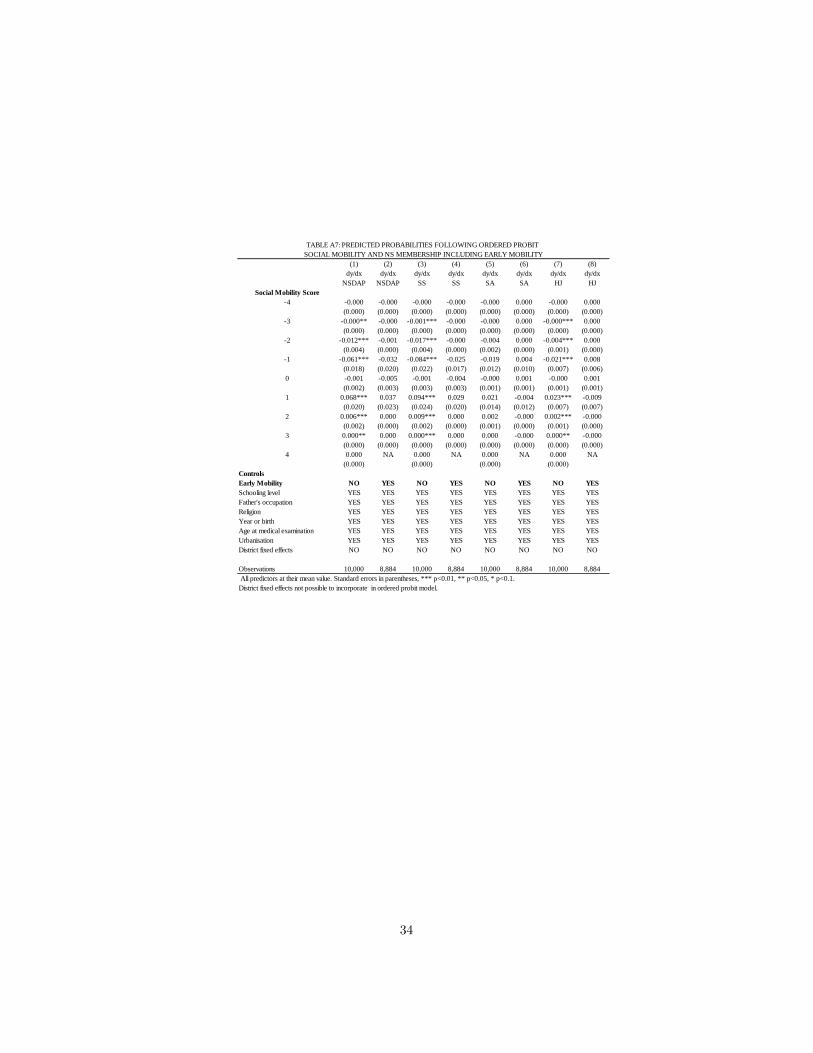
(1) (2) (3) (4) (5) (6) (7) (8)

dy/dx dy/dx dy/dx dy/dx dy/dx dy/dx dy/dx dy/dx

NSDAP NSDAP SS SS SA SA HJ HJ

Social Mobility Score

-4 -0.000 -0.000 -0.000 -0.000 -0.000 0.000 -0.000 0.000

(0.000) (0.000) (0.000) (0.000) (0.000) (0.000) (0.000) (0.000)

-3 -0.000** -0.000 -0.001*** -0.000 -0.000 0.000 -0.000*** 0.000

(0.000) (0.000) (0.000) (0.000) (0.000) (0.000) (0.000) (0.000)

-2 -0.012*** -0.001 -0.017*** -0.000 -0.004 0.000 -0.004*** 0.000

(0.004) (0.000) (0.004) (0.000) (0.002) (0.000) (0.001) (0.000)

-1 -0.061*** -0.032 -0.084*** -0.025 -0.019 0.004 -0.021*** 0.008

(0.018) (0.020) (0.022) (0.017) (0.012) (0.010) (0.007) (0.006)

0 -0.001 -0.005 -0.001 -0.004 -0.000 0.001 -0.000 0.001

(0.002) (0.003) (0.003) (0.003) (0.001) (0.001) (0.001) (0.001)

1 0.068*** 0.037 0.094*** 0.029 0.021 -0.004 0.023*** -0.009

(0.020) (0.023) (0.024) (0.020) (0.014) (0.012) (0.007) (0.007)

2 0.006*** 0.000 0.009*** 0.000 0.002 -0.000 0.002*** -0.000

(0.002) (0.000) (0.002) (0.000) (0.001) (0.000) (0.001) (0.000)

3 0.000** 0.000 0.000*** 0.000 0.000 -0.000 0.000** -0.000

(0.000) (0.000) (0.000) (0.000) (0.000) (0.000) (0.000) (0.000)

4 0.000 NA 0.000 NA 0.000 NA 0.000 NA

(0.000) (0.000) (0.000) (0.000)

Controls

Early Mobility NO YES NO YES NO YES NO YES

Schooling level YES YES YES YES YES YES YES YES

Father's occupation YES YES YES YES YES YES YES YES

Religion YES YES YES YES YES YES YES YES

Year or birth YES YES YES YES YES YES YES YES

Age at medical examination YES YES YES YES YES YES YES YES

Urbanisation YES YES YES YES YES YES YES YES

District fixed effects NO NO NO NO NO NO NO NO

Observations 10,000 8,884 10,000 8,884 10,000 8,884 10,000 8,884

All predictors at their mean value. Standard errors in parentheses, *** p<0.01, ** p<0.05, * p<0.1.

District fixed effects not possible to incorporate in ordered probit model.

TABLE A7: PREDICTED PROBABILITIES FOLLOWING ORDERED PROBIT

SOCIAL MOBILITY AND NS MEMBERSHIP INCLUDING EARLY MOBILITY

34