quasiparticle self-consistent gw method for the · pdf filequasiparticle self-consistent gw...

Top Curr Chem (2014)DOI: 10.1007/128_2013_460# Springer-Verlag Berlin Heidelberg 2014

Quasiparticle Self-Consistent GW Method

for the Spectral Properties of Complex

Materials

Fabien Bruneval and Matteo Gatti

Abstract The GW approximation to the formally exact many-body perturbation

theory has been applied successfully to materials for several decades. Since the

practical calculations are extremely cumbersome, the GW self-energy is most

commonly evaluated using a first-order perturbative approach: This is the

so-called G0W0 scheme. However, the G0W0 approximation depends heavily on

the mean-field theory that is employed as a basis for the perturbation theory.

Recently, a procedure to reach a kind of self-consistency within the GW framework

has been proposed. The quasiparticle self-consistent GW (QSGW) approximation

retains some positive aspects of a self-consistent approach, but circumvents the

intricacies of the complete GW theory, which is inconveniently based on a

non-Hermitian and dynamical self-energy. This new scheme allows one to sur-

mount most of the flaws of the usual G0W0 at a moderate calculation cost and at a

reasonable implementation burden. In particular, the issues of small band gap

semiconductors, of large band gap insulators, and of some transition metal oxides

are then cured. The QSGW method broadens the range of materials for which the

spectral properties can be predicted with confidence.

Keywords Electronic structure � Ab initio calculations � Many-body perturbation

theory � GW approximation

F. Bruneval

CEA, DEN, Service de Recherches de Metallurgie Physique, 91191, Gif-sur-Yvette, France

e-mail: [email protected]

M. Gatti (*)

Laboratoire des Solides Irradies, Ecole Polytechnique, CNRS-CEA/DSM, 91128, Palaiseau,

France

European Theoretical Spectroscopy Facility (ETSF)

Synchrotron SOLEIL, L’Orme des Merisiers, Saint-Aubin, BP 48, 91192,

Gif-sur-Yvette, France

e-mail: [email protected]

mailto:[email protected]

mailto:[email protected]

Contents

1 Photoemission Spectroscopy and Methods for Electronic Structure Calculations

2 Theoretical Survival Kit in GW Environment

2.1 Green’s Function G and Self-Energy Σ2.2 The Screened Coulomb Interaction W2.3 Hedin’s Equations and the GW Approximation

2.4 Practical Calculation of the GW Self-Energy: The G0W0 Approach

3 Beyond G0W0

3.1 Which Starting Point?

3.2 Energy Scales

3.3 Quasiparticle Wavefunctions

4 Quasiparticle Self-Consistent GW4.1 Full Self-Consistent GW4.2 The QSGW Approximation to the GW Self-Energy

4.3 Practical Implementation of the QSGW Method

4.4 Results

5 Relation with Alternative Self-Consistent Schemes

5.1 Energy-Only Self-Consistency

5.2 Alternatives to the QSGW: COHSEX and Others

5.3 Hybrid Functionals and LDA+U

6 Conclusions and Outlook

References

1 Photoemission Spectroscopy and Methods for Electronic

Structure Calculations

Photoemission (PES) is one of the most powerful spectroscopy tools that probe the

electronic properties of materials [1, 2]. Direct photoemission is a photon-in

electron-out technique: the energy of an incoming photon is used to extract an

electron (that is called the photoelectron) from the sample. If N is the initial

number of electrons, the electronic system after the electron removal is left in an

(N � 1)-electron state, which can be the ground state or an excited state. By

measuring the kinetic energy of the photoelectron, one obtains the ionization

energies of the electrons in the system (i.e., the energy required to remove an

electron, or, equivalently, to create a hole). The affinity energies (i.e., the energy

gained to add an electron to the system) can be analogously obtained by means of

inverse photoemission, which is an electron-in photon-out technique. Electron

addition and removal energies together define the electronic structure of a material

(e.g., its band gap). In particular, when the momentum (and possibly the spin) of the

photoelectron is also measured, as in angular-resolved photoemission (ARPES),

one gets access to the band structure of the material.

From the theoretical point of view, an accurate description of photoemission

spectra is still a great challenge today [3–8]. In the sudden approximation one

F. Bruneval and M. Gatti

assumes that the photoelectron is immediately decoupled from the sample. In this

approximation the measured photocurrent Jk(ω), which is the probability per unit

time of emitting an electron with momentum k and kinetic energy Ek when the

sample is irradiated with photons of frequency ω, is given by [5]

Jk ωð Þ ¼Xi

Δkij j2Aii Ek � ωð Þ, ð1Þ

where we have introduced the matrix elements of the spectral function A(ω) (forω < μ, where μ is the Fermi energy), which are weighted by the photoemission

matrix elements Δki that describe the coupling with the photons. Here we have also

assumed that there exists a one-particle basis in which A, rigorously defined as the

imaginary part of the one-particle Green’s function G (see Sect. 2), is diagonal.

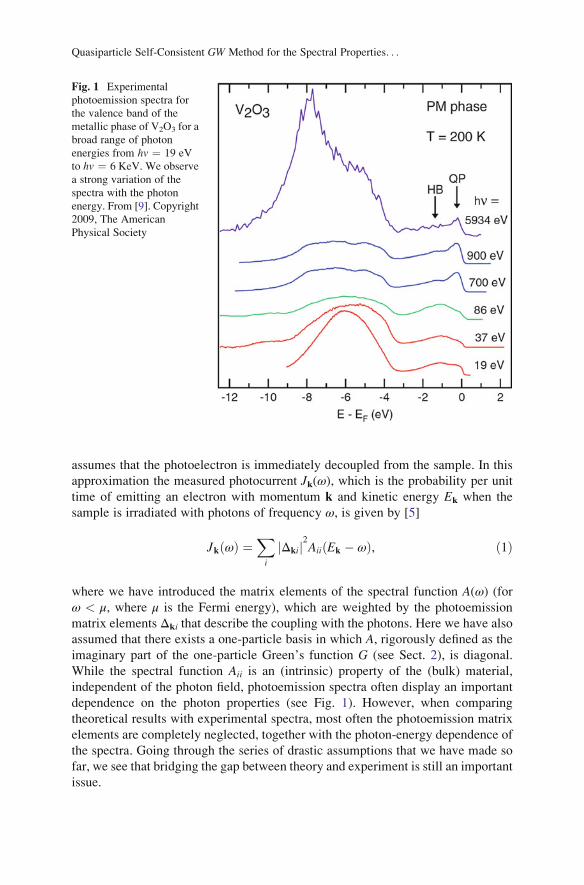
While the spectral function Aii is an (intrinsic) property of the (bulk) material,

independent of the photon field, photoemission spectra often display an important

dependence on the photon properties (see Fig. 1). However, when comparing

theoretical results with experimental spectra, most often the photoemission matrix

elements are completely neglected, together with the photon-energy dependence of

the spectra. Going through the series of drastic assumptions that we have made so

far, we see that bridging the gap between theory and experiment is still an important

issue.

Fig. 1 Experimental

photoemission spectra for

the valence band of the

metallic phase of V2O3 for a

broad range of photon

energies from hv ¼ 19 eV

to hv ¼ 6 KeV. We observe

a strong variation of the

spectra with the photon

energy. From [9]. Copyright

2009, The American

Physical Society

Quasiparticle Self-Consistent GW Method for the Spectral Properties. . .

In the following we will confine our discussion to the electronic properties

contained in the spectral function A. In an independent-particle picture the spectral

function for occupied states is simply Aii(ω) ¼ δ(ω � εi)θ(μ � ω) and the

photocurrent

Jk ωð Þ ¼Xocci

δ Ek � ω� εið Þ ð2Þ

is hence described by the density of occupied states evaluated at the energy Ek � ω,and is given by a series of delta peaks corresponding to the energies εi of the

one-particle Hamiltonian. By measuring the kinetic energy of the photoelectron, in

an independent-particle picture one would obtain directly the energy of the

one-particle level that the electron was occupying before being extracted from the

sample. More realistically, as a consequence of the electronic interactions, the delta

peaks in the spectral function acquire a finite width, which corresponds to the finite

lifetime of the excitation in the electronic system. Generally a broadened peak is

still prominent in the spectrum, having a weight Z (called the renormalization

factor) as large as 0.6–0.7 (a delta peak has Z ¼ 1). In these situations one

associates the peak with a quasiparticle (QP) excitation. The collection of the

energy positions of the quasiparticle peaks defines the band structure of the

material, which is most often the target of the calculations.

However, beyond a quasiparticle picture, the spectral function is generally much

richer. In fact, features with lower intensities (the satellites or side bands) are

often visible in the spectra. They correspond to situations in which the electronic

system is left in an (N � 1)-electron excited state which cannot be described by a

quasi-hole. Indeed, together with the electron removal, additional excitations

(e.g., plasmons) can also be induced in the system by the absorption of the photon.

Clearly a calculation of quasiparticle energies only is unable to describe satellites,

including Hubbard side bands, which are, by definition, a signature of many-body

effects beyond a band-structure description.

Density-functional theory (DFT) [10] is a ground-state theory and hence is not

appropriate to describe excitation energies measured in photoemission. In the

Kohn–Sham scheme [11] the ground-state density and the ground-state total energy

are obtained from a set of fictitious noninteracting electrons. Unfortunately, the

eigenvalues εi of the Kohn–Sham equation

�∇2

2þ Vext rð Þ þ VH rð Þ þ Vxc rð Þ

� �ϕi rð Þ ¼ εiϕi rð Þ, ð3Þ

where Vext, VH, and Vxc are respectively the external, Hartree, and exchange-

correlation potentials, cannot be interpreted as the additional or removal energies

measured in photoemission [12] (except for the HOMO level [13]). In practical

applications, the Kohn–Sham band gaps are most commonly smaller than

the experimental values. The exact quasiparticle band gap is defined as


[E(N + 1) � E(N )] � [E(N ) � E(N � 1)], where E(M ) is the ground-state total

energy of M electrons. In finite systems in the “self-consistent field” (Δ-SCF)scheme, these total energies for N, N � 1 electrons can be calculated explicitly

and approximations to Vxc can give good results for the band gaps, since they can

describe Hartree relaxation effects well [14]. The variation of the electron density

δρ for adding or removing an electron scales as 1/N: thus in an infinite system

δρ ! 0. In this limit the Δ-SCF scheme yields, with analytic functionals of the

density such the local-density approximation (LDA) [11], the Kohn–Sham band

gap [15]. In exact Kohn–Sham theory a nonanalytic, discontinuous change in Vxc

with respect to change in the electron number must be present [16–18].

Even in the homogeneous electron gas, where the local-density approximation is

exact for the total energies by definition, the discontinuity of the momentum

distribution at the Fermi surface (which corresponds to the renormalization factor

Z ) and spectral properties such as lifetimes and satellites remain inaccessible in the

Kohn–Sham formalism [19, 20]. The momentum distribution, for instance, can be

accurately calculated using Quantum Monte Carlo (QMC) techniques [19], but

excitations contained in the spectral function cannot be easily calculated in QMC at

the moment. Accurate quantum chemical methods, such as full configuration

interaction or coupled-cluster techniques, have been developed for molecular

systems, but until recently they have not been explored in solids for their high

computational complexity [21].

In spectroscopy one is often interested in specific answers to limited questions

and there is no need to calculate the full many-body wavefunction, which contains

more information than necessary. A successful strategy is hence to introduce

suitable quantities with a reduced number of degrees of freedom that are able to

provide the desired spectra. A key quantity is the spectral function – see (1) – which

can be calculated from the Green’s function G:

Aii ωð Þ ¼ 1

π

��ImGii ωð Þ��: ð4Þ

Many-body perturbation theory (MBPT) has traditionally been the framework in

which different approaches have been developed to calculate G. We can refer to the

various textbooks for a general introduction (see, e.g., [22–24]). Within MBPT,

Hedin’s GW approximation (GWA) [25] represents the state-of-the-art for the

calculation of band structures in a large variety of materials. Besides the early

review work by Hedin and Lundqvist [26], other in-depth reviews were published

around the year 2000 [14, 27, 28]. Since then the number of applications has

exploded, reaching more and more complicated materials such as interfaces [29],

surfaces with adsorbates (see, e.g., [30–32]), or defects in bulk materials (see,

e.g., [33–38]), and extending to other areas like quantum transport (see,

e.g., [39–43]). Moreover, the field itself has experienced several advances, both

from the technical and the fundamental points of view. For instance:


• Computational schemes that avoid sums of part or all the empty states have

recently been proposed (see, e.g., [44–49]).

• Pathologies and limits of the GWA (e.g., the self-screening problem and the

wrong atomic limit of the Hubbard model) and ways to go beyondGW have been

explored (see, e.g., [34, 50–54]).

• The GWA has been extended in various ways to account for phenomena not

contained in it. Examples include the cumulant expansion (see, e.g., [55, 56]),

the T matrix approximation (see, e.g., [57–59]), approaches developed starting

from the Hubbard model, like dynamical mean field theory (DMFT) [60], or with

the calculation of vibrational excitations [61, 62].

• Another emerging research line in recent years has been the application of the

GWA to non-equilibrium situations by means of the solution of the Baym–

Kadanoff equations (see, e.g., [42, 63–65]).

In this chapter we will focus on the approaches that have been developed in the

last decade to go beyond the perturbative G0W0 scheme (see Sect. 2), which has

been the standard implementation for GW calculations in real materials. We will

focus on the calculation of spectral properties (for instance we will not deal with

calculations of ground-state total energies; see, e.g., [66–70]). While advanced

computational schemes allow one to deal with more complicated materials

(e.g., with a larger number of atoms), beyond-G0W0 approaches have led to a

qualitative breakthrough in ab initio calculations of spectral properties of more

complex materials, such as those containing localized d or f electrons, also includ-

ing the challenging class of strongly correlated materials. In particular, in the

following we will discuss why (see Sect. 3) and how (see Sects. 4 and 5) to go

beyond G0W0, notably by means of the quasiparticle self-consistent GW (QSGW)

method introduced in 2004 by Faleev et al. [71]. Finally, we will conclude the

chapter by presenting a brief discussion of the new prospects that QSGW has

opened in the field.

2 Theoretical Survival Kit in GW Environment

2.1 Green’s Function G and Self-Energy Σ

The single-particle Green’s function G is the most basic ingredient of MBPT. The

time-ordered Green’s function describes the propagation of an extra electron in an

electronic system for positive times and the propagation of a missing electron

(i.e., a hole) for negative times1:

1 Here the spin degrees of freedom are omitted for simplicity. The generalization is however

straightforward.


iG rt, r0t0ð Þ ¼ θ�t� t0

�N0

��ψ rtð Þψ{ r0t0ð Þ��N0� ��θ t0 � tð Þ N0

��ψ{ r0t0ð Þψ rtð Þ��N0� �,

ð5Þ

where |N0i denotes the exact ground-state wavefunction of an N electron system, ψand ψ{ are the annihilation/creation field operators in the Heisenberg picture, and θis the step function.

The physical meaning of G becomes clear when inserting the closure relation in

between the two field operators and taking a Fourier transform in time. The

so-called Lehmann representation reads

G r, r0,ωð Þ ¼Xi

f i rð Þf �i r0ð Þω� Ei

: ð6Þ

The poles of G are located at the energies Ei:

Ei ¼ ENþ1i � EN0 � iη when Ei > μ¼ EN0 � EN�1i þ iη when Ei < μ,

ð7Þ

where the energies EN � 1i are the exact eigenenergies of the N � 1 electron system

and i is the index labeling the exact eigenvectors of both the N � 1 and N + 1

electron systems. The ubiquitous vanishing positive η has naturally arisen from the

Fourier transform of the step functions. In a solid, the discrete set of poles in (6)

merges into a branch-cut. The so-called Lehmann amplitudes fi are then defined as

f i rð Þ ¼ N0��ψ r0ð Þ��N þ 1i

� �when Ei > μ

¼ N � 1i��ψ r0ð Þ��N0� �

when Ei < μ:ð8Þ

Note that the Lehmann amplitudes fi are not mutually orthogonal. From this

representation we see that the poles Ei carry the exact ionization energies of

electrons in the system or the exact affinity energies. The analytical structure of

G is also made clear: the poles lie slightly above the real axis for Ei < μ and slightlybelow for Ei > μ. The poles can be directly compared to the peaks obtained from a

photoemission or inverse photoemission experiment (see Sect. 1).

BecauseG is the fundamental quantity, a great deal of effort has been put in to its

evaluation in a many-body context. This poses a very large challenge since equation

of motion for G involves the two-particle Green’s function. Its equation of motion

in turn involves the three-particle Green’s function, and so on. The standard remedy

in MBPT is to break this hierarchy by introducing an effective operator, the self-

energy Σ. As Schwinger showed, by introducing an auxiliary external field U(rt)that is set to zero at the end, it is possible to express formally the two-particle

Green’s function as a function of the one-particle Green’s function [72]. This results

in an equation of motion for G alone:


ðdr0 ω� h0 rð Þ � VH rð Þ½ �δ r� r0ð Þ � Σðr, r0,ωÞf gGðr0, r00,ωÞ ¼ δðr� r00Þ: ð9Þ

Here h0 is the non-interacting Hamiltonian and VH the Hartree potential – see (3).

Note that the self-energy Σ hides all the complexity of the original problem and thus

is a non-local, dynamical and non-Hermitian operator. When Σ ¼ 0 the Green’s

function G0 is simply the resolvent of the Hartree Hamiltonian: G�10 ¼ ω � h0 �

VH. We refer the reader to the review articles of Strinati [72] or of Hedin and

Lundqvist [26] for further details.

Dyson’s equation results by multiplying (9) by G0:

Gðr; r0;ωÞ ¼ G0ðr; r0;ωÞþðdr1dr2G0ðr; r1;ωÞΣ r1; r2;ωð ÞGðr2; r0;ωÞ: ð10Þ

This equation establishes the link between the Hartree Green’s function G0

(easily calculated) and the fully interacting Green’s function G (very hard to

calculate) through the self-energy Σ.The purpose of MBPT is then to provide approximations with increasing

accuracy for the self-energy. The Coulomb interaction between electrons

v r� r0ð Þ ¼ 1

r� r0j j ð11Þ

is considered as the perturbation with respect to the independent-particle case. The

first-order contribution to the self-energy is nothing else but the Fock exchange

operator (the Hartree potential is already taken into account by G0). This level of

approximation is widely used for atoms and molecules, and in quantum chemistry

perturbative methods in v with respect to Hartree–Fock are known as Møller–Plesset

perturbation theory [73]. However, for the homogeneous electron gas, Hartree–Fock

yields an anomalous zero density of states at the Fermi level. There is therefore a

stringent need for higher order terms for periodic systems. Unfortunately, the ana-

lytical evaluation of one of the two second-order contributions is not finite in the case

of the homogeneous electron gas [22, 23]. Perturbation theory is thus not justified.

How should one proceed to circumvent this problem, especially for periodic systems?

2.2 The Screened Coulomb Interaction W

This divergence can be addressed in an effective manner by introducing a screened

counterpart to the Coulomb interaction v. Other electrons act as a dielectric medium

that reduces the interaction between any pair. It is common sense that the interac-

tion between charges is not the same in vacuum as in a dielectric medium. At the

macroscopic scale this is measured by the dielectric constant of the medium. At the

microscopic scale the screening of the Coulomb interaction is given by


Wðr; r0;ωÞ ¼ðdr1ε

�1ðr; r1;ωÞv r1 � r0ð Þ, ð12Þ

where the microscopic dielectric matrix ε� 1 has been introduced. ε is linked to the

macroscopic dielectric function εM [74, 75], which is a measurable quantity. For

instance, � Imε�1M is called the loss function and can be measured by electron

energy loss spectroscopy (EELS) or inelastic X-ray scattering (IXS).

So far, the expression of the dielectric matrix has not been specified. Neverthe-

less, one can still analyze the physical meaning of the dynamically screened

Coulomb interaction W(r,r0,ω). The effective interaction between electrons in a

medium is decreased from v, the bare Coulomb interaction, to W the screened

interaction. A perturbation theory based on W rather than on v then makes much

more sense. However there is a price to pay: the screened interaction W is dynam-

ical, meaning that the screening is more effective for some frequencies than for

others. For metals, the static dielectric constant is infinite and consequently the

long-range component of W vanishes. This fixes the problem of the vanishing

density of states at the Fermi level predicted by Hartree–Fock theory for the

homogeneous electron gas. Conversely, in the high frequency limit, the screening

by the electrons becomes completely ineffective and the screened Coulomb inter-

action is simply the bare Coulomb interaction.

The additional complexity contained inW compared to v bears the hope that theperturbation theory is to be rapidly convergent. Maybe, as W already contains an

infinite sum of interactions v, just the first order in W will suffice, as proposed by

Hedin [25].

2.3 Hedin’s Equations and the GW Approximation

Employing W instead of v in the MBPT allowed Hedin to reformulate the exact

equations of the solution of the many-electron problem for the calculation of

G [25]. They read:

G 1; 2ð Þ ¼ G0 1; 2ð Þ þðd 34ð ÞG0 1; 3ð ÞΣ 3; 4ð ÞG 4; 2ð Þ ð13aÞ

Σ 1; 2ð Þ ¼ i

ðd 34ð ÞG 1; 3ð ÞW 1þ; 4ð ÞΓ 3; 2; 4ð Þ ð13bÞ

W 1; 2ð Þ ¼ðd 3ð Þε�1 1; 3ð Þv 3; 2ð Þ ð13cÞ

ε 1; 2ð Þ ¼ δ 1; 2ð Þ �ðd 3ð Þv 1; 3ð Þeχ 3; 2ð Þ ð13dÞ


eχ 1; 2ð Þ ¼ �i

ðd 34ð ÞG 1; 3ð ÞG 4; 1ð ÞΓ 3; 4; 2ð Þ ð13eÞ

Γ 1; 2; 3ð Þ ¼ δ 1; 2ð Þδ 1; 3ð Þ þðd 4567ð Þ δΣ 1; 2ð Þ

δG 4; 5ð ÞG 4; 6ð ÞG 7; 5ð ÞΓ 6; 7; 3ð Þ: ð13fÞ

Contracted indexes (1) ¼ (r1,t1,σ1) have been used for simplification. The index

1+ denotes the times t1 + η for a vanishing positive η. Most of the quantities have

been introduced earlier. eχ is the irreducible polarizability and Γ is the three-point

vertex function. These nonlinear equations are coupled. If solved self-consistently,

these equations form an exact scheme to obtain the solution of the many-body

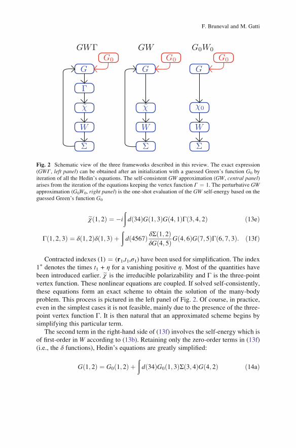
problem. This process is pictured in the left panel of Fig. 2. Of course, in practice,

even in the simplest cases it is not feasible, mainly due to the presence of the three-

point vertex function Γ. It is then natural that an approximated scheme begins by

simplifying this particular term.

The second term in the right-hand side of (13f) involves the self-energy which is

of first-order in W according to (13b). Retaining only the zero-order terms in (13f)

(i.e., the δ functions), Hedin’s equations are greatly simplified:

G 1; 2ð Þ ¼ G0 1; 2ð Þ þðd 34ð ÞG0 1; 3ð ÞΣ 3; 4ð ÞG 4; 2ð Þ ð14aÞ

Fig. 2 Schematic view of the three frameworks described in this review. The exact expression

(GWΓ, left panel) can be obtained after an initialization with a guessed Green’s function G0 by

iteration of all the Hedin’s equations. The self-consistent GW approximation (GW, central panel)arises from the iteration of the equations keeping the vertex function Γ ¼ 1. The perturbative GWapproximation (G0W0, right panel) is the one-shot evaluation of the GW self-energy based on the

guessed Green’s function G0


Σ 1; 2ð Þ ¼ iG 1; 2ð ÞW 1þ; 2ð Þ ð14bÞ

W 1; 2ð Þ ¼ðd 3ð Þε�1 1; 3ð Þv 3; 2ð Þ ð14cÞ

ε 1; 2ð Þ ¼ δ 1; 2ð Þ �ðd 3ð Þv 1; 3ð Þeχ 3; 2ð Þ ð14dÞ

eχ 1; 2ð Þ ¼ �iG 1; 2ð ÞG 2; 1ð Þ: ð14eÞ

The irreducible polarizability eχ is then a simple product of two Green’s

functions. This is the well known Random-Phase Approximation (RPA) to the

dielectric matrix. The self-energy is also much simplified: this is just the simple

product of G andW, giving the name to the GW approximation. It is of first-order in

W. The missing terms (second and higher orders in W ) are commonly named the

“vertex corrections”.

The set of equations (14a–14e) still requires a self-consistent treatment since

W and Σ depend onG, which is the quantity one needs to find. This is pictured in thecentral panel of Fig. 2. The practical implementation of these equations is still far

from obvious. This is the reason why for many years the GW self-energy has been

evaluated non-self-consistently.

2.4 Practical Calculation of the GW Self-Energy: The G0W0

Approach

It is usually impossible to evaluate the Green’s function self-consistently from

(14a–14e). However, let us imagine that mean-field theories such as Hartree–

Fock or Kohn–Sham provide a good description of the electronic system under

study. In a mean-field theory, the one-electron wavefunctions ϕi(r) and eigenvalues

ɛi allow one to evaluate the independent-particle Green’s function2 G0

G0 r; r0;ω

� � ¼ Xi

ϕi rð Þϕ∗i r0ð Þ

ω� εi þ iηsign εi � μð Þ : ð15Þ

The location of the poles of G0 are above the real axis for occupied states and

below for empty states. As a consequence, eχ and then W can be readily evaluated

from this expression of G0. Let us label this evaluation of the irreducible polariz-

ability χ0 and of the screened Coulomb interaction,W0. Finally, the GW self-energy

is obtained as the convolution G0W0.

2G0 here can be understood as a generalization of the Hartree Green’s function introduced in

(10.2), and thus we keep the same notation for a distinct quantity. See also Sect. 2.1 for an

extended discussion.


The so-called G0W0 approach consists in stopping the procedure immediately

after the first evaluation of the self-energy, as shown in the right hand panel of

Fig. 2. This “one-shot” procedure is justified when the starting mean-field theory

used for G0 is accurate enough for the targeted property. The vast majority of the

GW applications for almost 50 years have been obtained with the G0W0 procedure.

Of course, the choice of the starting point is material dependent. The seminal paper

of Hedin [25] simply employed the free electron model to calculate the GW self-

energy for the homogeneous electron gas. The first application of GW to real solids

used either the Hartree–Fock approximation [76] or the local density approximation

[77]. For atoms, Shirley and Martin chose Hartree–Fock [78]. The rationale under-

lying the choice is the selection of the most accurate mean-field theory for the

specific system under scrutiny. This strategy is sometimes referred to as the “bestG,best W” approach (see Sect. 3.1).

In the quasiparticle approximation, the Dyson equation (10) becomes

�∇2

2þ Vext rð Þ þ VH rð Þ

� �ψ i rð Þ þ

ðdr

0Σ r; r

0;Ei

� �ψ i r

0ð Þ ¼ Eiψ i rð Þ ð16Þ

In the G0W0 framework one assumes that the quasiparticle wavefunctions ψ i can

be approximated by the Kohn–Sham orbitals ϕi. By comparing (3) and (16) one

finds that the quasiparticle energies Ei can be calculated as a first-order correction

with respect to the underlying mean-field starting point from

Ei ¼ εi þ ϕi

��Σ Eið Þ � Vxc

��ϕi

� �, ð17Þ

where Σ is the G0W0 self-energy. From a linearization of the frequency dependence

of Σ, one finally obtains

Ei ¼ εi þ Zi ϕi

��Σ εið Þ � Vxc

��ϕi

� �, ð18Þ

where the renormalization factors Zi are

Zi ¼ 1� hϕi

��∂Σ ωð Þ∂ω

��ω¼εi

��ϕii �1

: ð19Þ

In most G0W0 calculations the band structures are obtained using (18). One can

also calculate the spectral function defined in (4) from:

Aii ωð Þ ¼ 1

π

ϕi

��ImΣ ωð Þ��ϕi

� �� ω� εi � ϕi

��ReΣ ωð Þ � Vxc

��ϕi

� �� 2 þ ϕi

��ImΣ ωð Þ��ϕi

� �� 2 : ð20Þ

The spectral function has poles correspondence to the quasiparticle energies, i.e.,

when ω � εi � hϕi|ReΣ(ω) � Vxc|ϕii ¼ 0; cf. (17). The width of the quasiparticle

peak is given by ImΣ(ω), which is hence linked to the lifetime of the excitation

(defined as the inverse of its width). The spectral function can have other peaks, the


satellites, that originate from structures in ImΣ(ω). ω � εi � hϕi|ReΣ(ω) � Vxc|ϕiican also have additional zeroes, giving rise to satellites. Within the GWA this latter

kind of satellites has been called plasmarons [79, 80], but lately they have been

shown to be an artifact of the GWA [56, 81, 82]. In Hartree–Fock the self-energy is

Hermitian: ImΣ(ω) ¼ 0. Therefore quasiparticle peaks become delta functions (i.e.,

the lifetime of quasiparticle becomes infinite). Moreover, since the self-energy is

static, no other structures (e.g., satellites) can appear in the spectral function.

The GW self-energy can be split into a Fock exchange term Σx and a correlation

term Σc(ω): Σ(ω) ¼ Σx + Σc(ω). While Σx ¼ iGv is static, the evaluation of Σc(ω)requires the calculation of the convolution integral of G and Wp ¼ W � v:

Σc r1; r2;ωð Þ ¼ i

2π

ðdω

0eiηω

0G r1, r2,ωþ ω

0� �Wp r1; r2;ω

0� �: ð21Þ

Since Σc is obtained through the frequency integration (21), the fine details of the

energy dependence of Wp are often not important. In these cases one can approx-

imate the imaginary part of the inverse dielectric function ε� 1 as a single-pole

function in ω (plasmon-pole model) [83, 84]. Plasmon-pole models can be used for

calculating quasiparticle energies, but should be avoided for spectral functions

because, for example, they do not describe ImΣ correctly. In these cases the full-

frequency dependence of Σ is required and the frequency integration has to be

performed with care [85].

The spectral representation of Wp is given by [5]

Wp r1; r2;ωð Þ ¼ 2Xs

ωsWs r1; r2ð Þω2 � ωs � iηð Þ2 : ð22Þ

The poles of Wp are the energies ωs that correspond to neutral excitations

(electron-hole transitions and plasmons). By combining (22) with (15) and

performing the frequency integration (21), one finds that the G0W0 self-energy is

given by the sum of two terms:

ΣSEX r1; r2;ωð Þ ¼ �Xi

θ μ� εið Þϕi r1ð Þϕ∗i r2ð ÞW r1, r2,ω� εið Þ, ð23aÞ

ΣCOH r1; r2;ωð Þ ¼Xi

ϕi r1ð Þϕ∗i r2ð Þ

Xs

Ws r1; r2ð Þω� ωs � iηð Þ � εi

: ð23bÞ

The first term arises from the poles in G and the second from the poles in W.

Owing to the similarity of the first term with the Fock exchange, it is usually called

the “screened exchange” term. The second term is referred to as the “Coulomb-

hole” term [25]. If a further static approximation is carried out, this decomposition

gives rise to the so-called COHSEX (Coulomb hole plus screened exchange), first

introduced by Hedin [25, 79]. This static and Hermitian self-energy is obtained by

setting ω � εi ¼ 0 in ΣSEX(ω) and ΣCOH(ω). This corresponds to assuming that the


main contribution to the self-energy Σ(ω) stems from the states εi close to ω. Soω � εi is small compared to the main excitations in W which are at the plasmon

energies ωs [25, 79].

In the majority of practical cases the G0W0 scheme is largely sufficient to

evaluate successfully the GW self-energy. However for some cases it is not. This

review will focus precisely on those pathological cases.

3 Beyond G0W0

In this section we will present arguments to show why one should go beyond the

G0W0 scheme that has been introduced in the previous section. First of all, we will

discuss the criticisms that can be raised about G0W0 from the point of view of basicprinciples. Then we will consider a case study where the G0W0 scheme shows inpractice to be inadequate under different aspects. This practical example is VO2, a

prototypical transition metal oxide, which has been the subject of an intense debate

for the last 5 decades for its metal-insulator transition occurring just above room

temperature [86].

3.1 Which Starting Point?

The GW approximation can be seen to correspond to the first step of an iterative

solution of Hedin’s equations that takes as the starting point Σ ¼ 0 (see Fig. 2).

Therefore, in principle the GW self-energy should be built using a Green’s function

G calculated in the Hartree approximation (i.e., with Σ ¼ 0). However, the Hartree

approximation is generally inadequate, giving bad electron densities and

one-particle wavefunctions. Moreover, performing an additional step in the itera-

tive solution of Hedin’s equations leads to the inclusion of vertex corrections

beyond GW that are immediately very expensive from the computational point

of view.

One would rather like to remain within the GWA and find an alternative

strategy to evaluate the self-energy, discarding the idea of solving Hedin’s equa-

tions iteratively. This has been the approach followed in practice in the application

of the GWA to the calculations of band structures of real materials [18, 77,

83]. The idea is to build the GW self-energy with the best ingredients that can

be calculated from first-principles. Historically, in solids this led to the use of the

LDA or the GGA (alternatively, Hartree–Fock for atoms [78]) at the place of the

Hartree approximation. This was justified by the observation that in sp semi-

conductors and metals LDA wavefunctions are a good approximation to QP

wavefunctions [83] (see Sect. 2.4). A posteriori this choice was validated by the

good agreement of G0W0 results with experimental band gaps [27, 28].


Moreover, still in the spirit of the iterative solution of Hedin’s equations, one

could improve the starting point by setting Σ ¼ Vxc, instead of Σ ¼ 0 [83, 87]. This

would give a self-energy that still has a GW-like form. However, the Coulomb

interaction is now screened by an effective dielectric function that has a electron-

test-charge form, eε ¼ 1� vþ f xcð Þχ0, instead of the RPA ε used in the standard

GW approximation, ε ¼ 1 � vχ0. The main difference is that in the electron-test-

charge case the induced charge generates an exchange-correlation potential in

addition to the induced Coulomb potential that is already taken into account at

the RPA level. This approximation has been called “GWΓ” [87] because it contains,to some extent, vertex corrections beyond GW. It is consistently derived and

calculated using Kohn–Sham ingredients. It has been shown to give results that

are similar to (or slightly worse than) standard LDA-based GW [29, 52, 87, 88],

adding another argument in favor of the pragmatic “best G best W” approach.

Vertex corrections beyond the local approximation used to build vertex in the

“GWΓ” scheme [87] are still an open question under investigation [89, 90].

Anyway, this “best G best W” strategy clearly introduces a degree of arbitrar-

iness in the results. As any first-order perturbation scheme, theG0W0 results directly

depend on the quality of the starting point (i.e., the zero order of the perturbative

scheme). In general, Hartree–Fock overestimates and the LDA (or GGA) underes-

timates band gaps (and analogously HOMO-LUMO gaps in finite systems). G0W0

corrections improve with respect to the starting point, getting closer to experiment

from above if starting from Hartree–Fock, or from below if starting from LDA or

GGA. Therefore G0W0 results obtained from these two starting points generally

bracket the reference values, and starting from any hybrid functional mixing LDA

with Fock non-local exchange gives rise to intermediate results between the two.

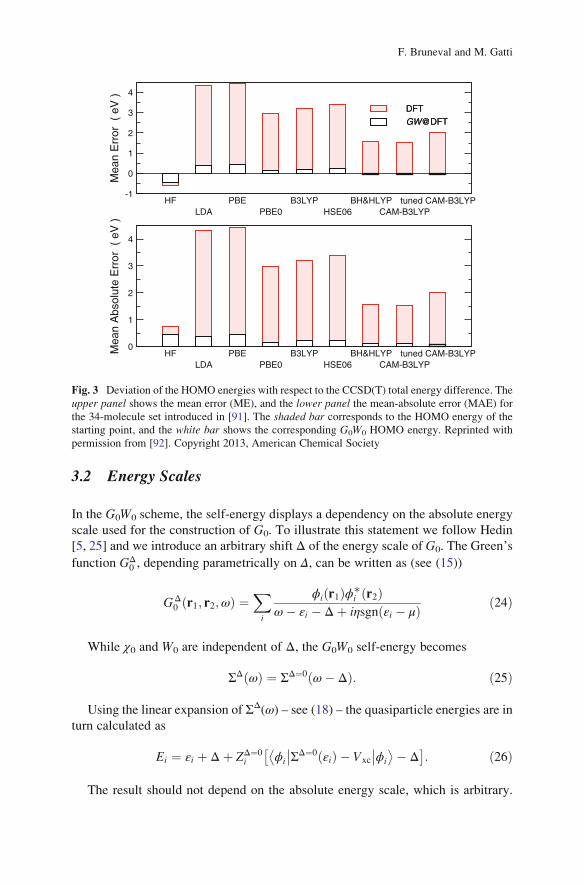
This observation is, for instance, illustrated for a benchmark of 34 small closed-

shell molecules in Fig. 3. Deviations from the reference quantum chemistry

CCSD(T) calculations are reported: each bar corresponds to a different approxima-

tion for the exchange-correlation functional used in the underlying mean-field

calculation, comprising local, semilocal, and several hybrid functionals [92]. Sim-

ilar results for atoms and molecules have recently been obtained, for instance also

in [91, 93–96], and these observations can be generalized to extended systems as

well.

Moreover, in contrast to the first applications of the LDA-based G0W0 scheme,

in recent years the investigation of more complex materials has shown severe

limitations of the G0W0 approach. Alternative starting points beyond LDA have

been put forward, either remaining in the Kohn–Sham scheme – e.g., using the

exact exchange approximation (EXX) [97, 98] or LDA+U [99, 100] – or moving to

a generalized Kohn–Sham scheme and adding a part of non-local Fock exchange –

e.g., using the Heyd–Scuseria–Ernzerhof (HSE) hybrid functional [101, 102]. In

most cases bad G0W0 results have been explained in terms of the inadequacy of the

underlying LDA starting point.


3.2 Energy Scales

In the G0W0 scheme, the self-energy displays a dependency on the absolute energy

scale used for the construction of G0. To illustrate this statement we follow Hedin

[5, 25] and we introduce an arbitrary shift Δ of the energy scale of G0. The Green’s

function GΔ0 , depending parametrically on Δ, can be written as (see (15))

GΔ0 r1; r2;ωð Þ ¼

Xi

ϕi r1ð Þϕ∗i r2ð Þ

ω� εi � Δþ iηsgn εi � μð Þ ð24Þ

While χ0 and W0 are independent of Δ, the G0W0 self-energy becomes

ΣΔ ωð Þ ¼ ΣΔ¼0 ω� Δð Þ: ð25Þ

Using the linear expansion of ΣΔ(ω) – see (18) – the quasiparticle energies are inturn calculated as

Ei ¼ εi þ Δþ ZΔ¼0i ϕi

��ΣΔ¼0 εið Þ � Vxc

��ϕi

� �� Δ� �

: ð26Þ

The result should not depend on the absolute energy scale, which is arbitrary.

HFLDA

PBEPBE0

B3LYPHSE06

BH&HLYPCAM-B3LYP

tuned CAM-B3LYP-1

0

1

2

3

4

Mea

n E

rror

( e

V )

DFT

GW@DFT

HFLDA

PBEPBE0

B3LYPHSE06

BH&HLYPCAM-B3LYP

tuned CAM-B3LYP0

1

2

3

4

Mea

n A

bsol

ute

Err

or (

eV

)DFT

GW@DFT

Fig. 3 Deviation of the HOMO energies with respect to the CCSD(T) total energy difference. The

upper panel shows the mean error (ME), and the lower panel the mean-absolute error (MAE) for

the 34-molecule set introduced in [91]. The shaded bar corresponds to the HOMO energy of the

starting point, and the white bar shows the corresponding G0W0 HOMO energy. Reprinted with

permission from [92]. Copyright 2013, American Chemical Society


On the contrary, here we see that shifting by Δ the energy scale of G0 leads to a

variation of the quasiparticle energies equal to (1 � ZiΔ ¼ 0)Δ. This is a conse-

quence of the fact that the self-energy in the GWA is dynamical, hence Zi 6¼ 1.

However, if the renormalization factors Zi do not change much from state to

state, as is generally the case in simple systems, this dependency on the absolute

energy scale of G0 has a tiny effect on the G0W0 band-structure results. In this

situation, in fact, changing arbitrarily the energy scale of G0 would only give a rigid

shift of the whole band structure.

In order to fix this problem, Hedin suggested setting the energy scale by

requiring a self-consistency at the Fermi level [5, 25]. This means setting Δ equal

to the matrix element of the self-energy at the Fermi level calculated with Δ ¼ 0.

A more general solution would be to calculate self-consistently the energies

entering Σ (and hence also the Fermi level).

A more severe consequence of this dependency on the energy scale can be found

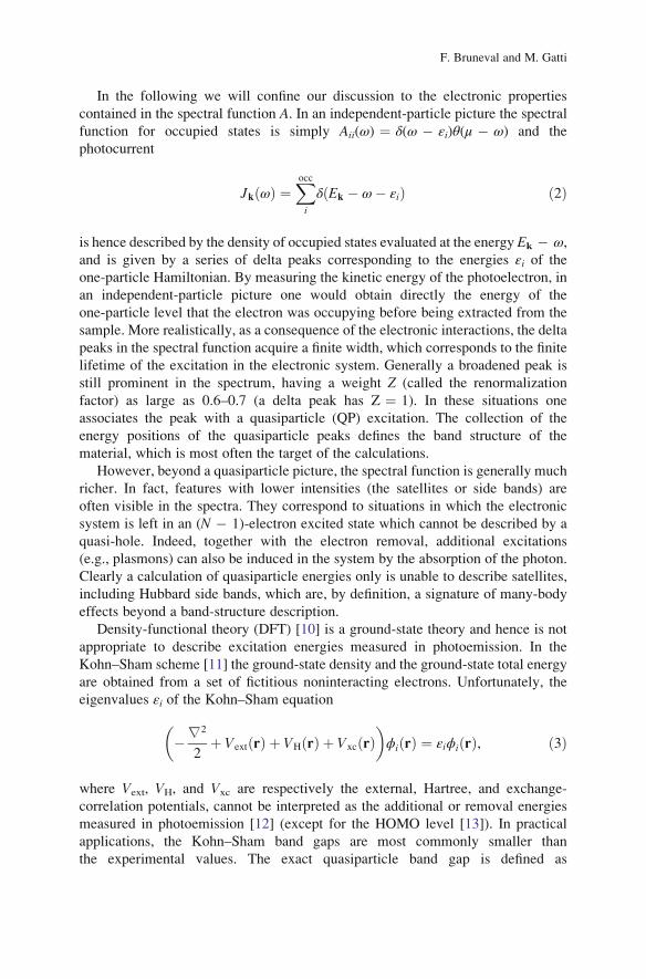
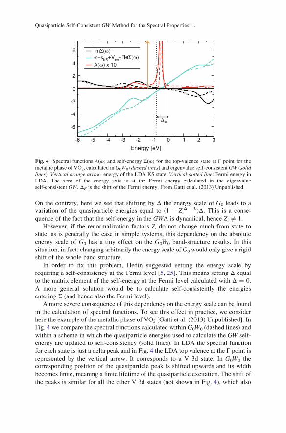
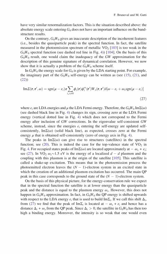
in the calculation of spectral functions. To see this effect in practice, we consider

here the example of the metallic phase of VO2 [Gatti et al. (2013) Unpublished]. In

Fig. 4 we compare the spectral functions calculated within G0W0 (dashed lines) and

within a scheme in which the quasiparticle energies used to calculate the GW self-

energy are updated to self-consistency (solid lines). In LDA the spectral function

for each state is just a delta peak and in Fig. 4 the LDA top valence at the Γ point is

represented by the vertical arrow. It corresponds to a V 3d state. In G0W0 the

corresponding position of the quasiparticle peak is shifted upwards and its width

becomes finite, meaning a finite lifetime of the quasiparticle excitation. The shift of

the peaks is similar for all the other V 3d states (not shown in Fig. 4), which also

-6 -5 -4 -3 -2 -1 0 1 2 3

Energy [eV]

-6

-4

-2

0

2

4

6

ΔF

ImΣ(ω)ω−εKS+Vxc−ReΣ(ω)A(ω) x 10

Fig. 4 Spectral functions A(ω) and self-energy Σ(ω) for the top-valence state at Γ point for the

metallic phase of VO2, calculated inG0W0 (dashed lines) and eigenvalue self-consistent GW (solidlines). Vertical orange arrow: energy of the LDA KS state. Vertical dotted line: Fermi energy in

LDA. The zero of the energy axis is at the Fermi energy calculated in the eigenvalue

self-consistent GW. ΔF is the shift of the Fermi energy. From Gatti et al. (2013) Unpublished


have very similar renormalization factors. This is the situation described above: the

absolute energy scale enteringG0 does not have an important influence on the band-

structure results.

On the contrary, G0W0 gives an inaccurate description of the incoherent features

(i.e., besides the quasiparticle peak) in the spectral function. In fact, the satellite

measured in the photoemission spectrum of metallic VO2 [103] is too weak in the

G0W0 spectral function (see dashed red line in Fig. 4)) [104]. On the basis of this

G0W0 result, one would claim the inadequacy of the GW approximation for the

description of this genuine signature of dynamical correlation. However, we now

show that it is actually a problem of the G0W0 scheme itself.

InG0W0 the energy scale forG0 is given by the LDA starting point. For example,

the imaginary part of the G0W0 self-energy can be written as (see (15), (21), and

(22))

ImΣðr; r0;ωÞ ¼ sgn μ� εið ÞπXi, s 6¼0

ϕi rð Þϕ∗i ðr0ÞWsðr; r0Þδ ω� εi þ ωssgn μ� εið Þ½ �

ð27Þ

where εi are LDA energies and μ the LDA Fermi energy. Therefore, theG0W0 ImΣ(ω)(see dashed black line in Fig. 4) changes its sign, crossing zero at the LDA Fermi

energy (vertical dotted line in Fig. 4) which does not correspond to the Fermi

energy after inclusion of GW corrections. In the eigenvalue self-consistent GWscheme, instead, since the energies εi entering the self-energy are updated self-

consistently, ImΣ(ω) (solid black line), as expected, crosses zero at the Fermi

energy μ that is obtained self-consistently (zero of energy axis in Fig. 4).

The peaks in ImΣ(ω) can give rise to structures (satellites) in the spectral

function; see (20). This is indeed the case for the top-valence state of VO2 in

Fig. 4. For occupied states peaks of ImΣ(ω) are located approximately at� ωs + εi;see (27). In VO2 ωs�1.5 eV is the energy of a localized d � d plasmon and the

coupling with this plasmon is at the origin of the satellite [105]. This satellite is

called a shake-up excitation. This means that in the photoemission process the

photoemitted electron leaves the (N � 1)-electron system in an excited state in

which the creation of an additional plasmon excitation has occurred. The main QP

peak in this case corresponds to the ground state of the (N � 1)-electron system.

On the basis of this physical picture, for the energy-conservation rule we expect

that in the spectral function the satellite is at lower energy than the quasiparticle

peak and the distance is equal to the plasmon energy ωs. However, this does not

happen in G0W0 approximation. In fact, in G0W0 the QP energy is shifted upwards

with respect to the LDA energy εi that is used to build ImΣi. If we call this shift Δi,

from (27) we find that the peak of ImΣi is located at � ωs + εi and hence has a

distance Δi + ωs from the QP peak. Since Δi > 0, the satellite in G0W0 has then too

high a binding energy. Moreover, the intensity is so weak that one would even


conclude that there is no satellite in GW [104]. Instead, in the eigenvalue self-

consistent GW scheme the satellite gets closer to the QP peak (see solid red line),

because at self-consistency Δi ¼ 0. The distance between the satellite and the QP

peak becomes correctly � ωs, i.e., the energy of the plasmon. Moreover, the

intensity of the satellite is enhanced with respect to G0W0 due to the fact that

|(ω � εi � (ReΣi(ω) � Vxci )| becomes smaller (compare solid and dashed cyan

lines). In conclusion, the eigenvalue-self-consistent GW scheme gives a correct

description of the low-energy satellite [Gatti et al. (2013) Unpublished], in contrast

to G0W0.

The example just discussed shows that conclusions about spectral functions

should not be based on calculations at the G0W0 level, especially if one is interested

in spectral properties close to the Fermi level and the self-energy induces a

non-negligible shift of the positions of the peaks with respect to the LDA starting

point. In fact the same problem has been observed in other situations, such as

Hubbard chains [106] or SrVO3, another prototypical strongly correlated metal

[107]. This conclusion is also relevant when GW is combined with other methods

that calculate spectral functions, such as dynamical mean field theory (DMFT).

3.3 Quasiparticle Wavefunctions

The G0W0 scheme is based on the hypothesis that QP wavefunctions can be

approximated by LDA orbitals; see (17). This assumption holds for simple semi-

conductors and metals and has been investigated in depth, e.g., for bulk silicon

[83]. However, it has been known for a long time that it can be questionable for

finite systems [108] and surfaces [109–111]. In simple systems like bulk silicon the

LDA conduction wave functions have also recently been shown to be of signifi-

cantly poorer quality, in particular away from highly symmetric points of the

Brillouin zone [112]. Here, through the case study of the insulating phase of VO2,

we discuss a situation in which the G0W0 perturbation theory breaks down

completely [105]. Similar problems occur when LDA produces a wrong ordering

of the bands (see, e.g., [113, 114]).

Across the metal-insulator transition, VO2 also undergoes a structural phase

transition from rutile (metal) to monoclinic (insulator). This is accompanied by the

formation of V–V dimers along the rutile c axis, resulting into a doubling of the unitcell. The LDA underestimates the bonding-antibonding splitting of the V 3d states

associated with the formation of these V–V dimers and in turn the band structure is

metallic [115]. Alternatively, the metallic LDA band structure has been interpreted

as the proof of the strongly correlated nature of VO2 [116].

In apparent support of the hypothesis of “strong correlation,” G0W0 based on

LDA also fails to open the gap. In order to get rid of the LDA starting point, QP

wavefunctions have been calculated self-consistently in the COHSEX approxima-

tion [105]. This self-consistent quasiparticle calculation does succeed in opening a


gap (0.8 eV, quite close to the experimental value of 0.6 eV). In contrast, in a

COHSEX calculation where the wavefunctions are constrained to be the LDA ones

and only the energies are updated self-consistently, a gap close to zero is found: the

change of the wavefunctions with respect to the LDA ones is thus of utmost

importance.

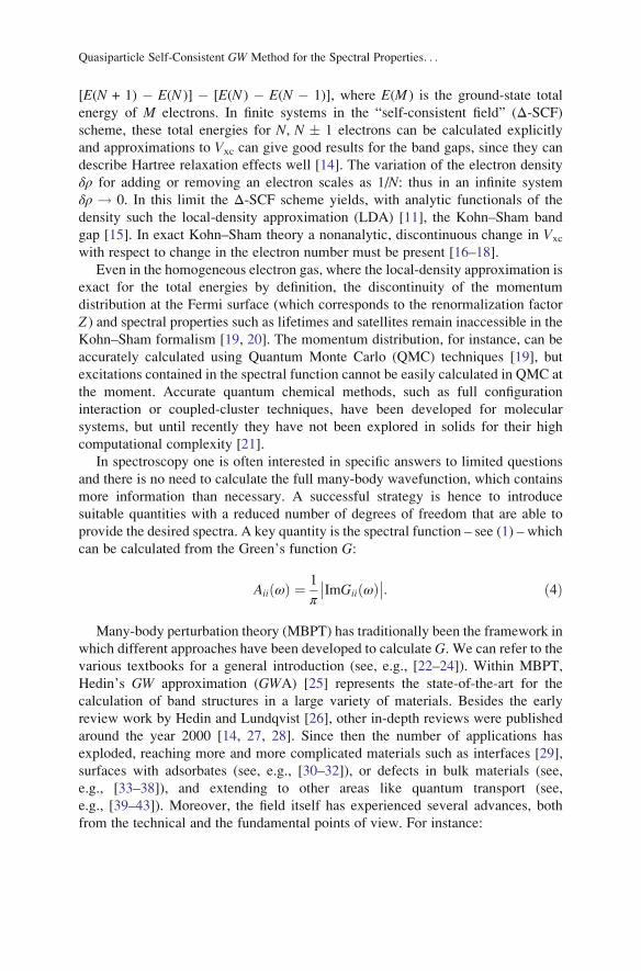
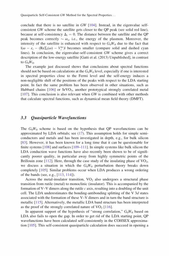
In Fig. 5 the LDA electron density for the top valence bands is plotted (see the

left panel). It represents the V a1g states that derive from the V–V dimer bonding

states and are hence highly polarized along the V–V dimer axis (the vertical c axisin the figure). The self-consistent QP COHSEX calculation results in the enhance-

ment of this anisotropy, inducing a stronger bonding character to the top valence

wavefunctions. Therefore if the orbital redistribution associated with the formation

of V–V dimers is underestimated, as happens in LDA, the system remains metallic.

Since LDA orbitals are not a sufficiently good approximation of the QP

wavefunctions at the Fermi level, the G0W0 perturbative scheme on top of LDA

is not valid in the present situation. Improved QP wavefunctions are instead

obtained in the COHSEX approximation, which can be used for a subsequent

G0W0 calculation.

More generally, this conclusion about the failure of G0W0 holds for d and felectron states for which the LDA tends to produce too delocalized wavefunctions

[71, 113, 117–126]. The Fock exchange term of the self-energy is essential in these

situations to cure this delocalization error [126].

Fig. 5 (Left panel)Isosurface of the LDA

electron density for the top

valence V 3d bands in

insulating VO2. It is a V–V

dimer bonding a1g state,highly polarized along the

cc axis (vertical axis in the

figure). (Right panel)Difference between

COHSEX and LDA

electron density for the

same states. Yellow surfacesare for positive variations

and purple for negativeones. The c-axispolarization increases for

COHSEX wavefunctions.

See [105]


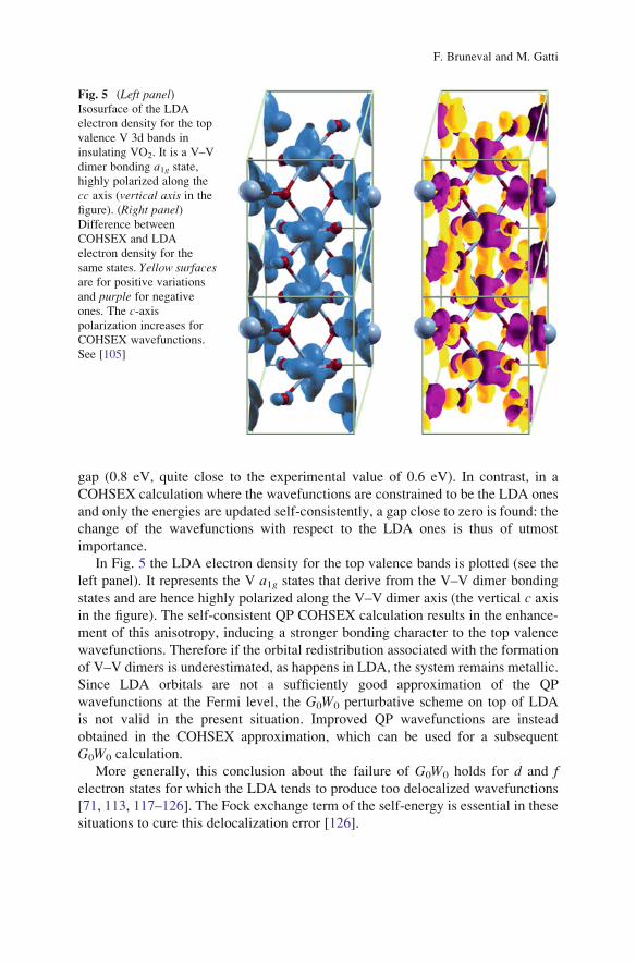
Finally, in Fig. 6 we illustrate the effect of using QP wavefunctions instead of

LDA ones in the optical spectra of insulating VO2 [Gatti et al. (2013) Unpublished].

Here the absorption spectrum, given by the imaginary part of the dielectric function

ɛM, is obtained as a sum over independent vertical transitions from valence to

conduction states, corresponding to Fermi’s golden rule in the independent-particle

picture. The energies of these transition are calculated using the COHSEX+ G0W0

results that correctly produce an insulator in VO2 [105]; hence the onset of the

optical spectrum is at a finite energy. However, the spectrum calculated with LDA

wavefunctions starts with a peak of huge intensity (see yellow line). This huge peak

derives from the shift of the metallic Drude peak at ω � 0 in the spectrum

calculated with metallic LDA eigenvalues. In order to understand this problem

better, we write the oscillators strengths for vanishing q that determine the absorp-

tion spectrum by using k � p perturbation theory [127]:

limq!0

ϕvk

��e�iq:r��ϕckþq

� � ¼ limq!0

iq � ϕvk

�� HKS; r� ��ϕck

� �εck � εvk

, ð28Þ

with HKSϕi ¼ εiϕi. If LDA wavefunctions are used to calculate the oscillator

strengths (28), then the energy differences appearing at the denominator in (28)

are by definition also to be calculated in LDA. Therefore, since VO2 is metallic in

LDA, for the first transitions the denominator is vanishingly small. In turn, the

oscillator strength of the first peak remains very high, although the position is givencorrectly by COHSEX+ G0W0 energy differences. Thus the wrong oscillator

strength is due to the use of LDA wavefunctions and is corrected by using QP

wavefunctions calculated in the self-consistent COHSEX scheme (see blue line in

Fig. 6). The effect is drastic for VO2, but one should expect similar behavior

whenever the opening of a small bandgap is accompanied by a change of

wavefunctions.

0 0.5 1 1.5 2 2.5 3 3.5 4 4.5 5

Energy [eV]

0

5

10

15

20

25

30

35

40

Im ε

LDA wavefunctionsCOHSEX wavefunctions

0 1 2 3 4 50

50

100

150

200

250Fig. 6 Absorption

spectrum Im E of insulatingVO2, calculated in the

independent-particle

approximation using

COHSEX+ G0W0 energies

and LDA (yellow line in the

main panel and in the inset)or COHSEX (blue line)wavefunctions. See Gatti

et al. (2013) Unpublished


4 Quasiparticle Self-Consistent GW

For all the aforementioned reasons, it seems very attractive to get rid of the mean-

field starting point which pervasively affects all the G0W0 results. The natural way

to do so would be to turn to self-consistent GW calculations, as pictured in the

central panel of Fig. 2. However, the full self-consistent GW approach suffers from

many drawbacks as we will show in the next paragraph. This is the main reason why

Faleev, Kotani, and van Schilfgaarde introduced in 2004 the so-called “Quasipar-

ticle-Self-consistent GW” scheme [71], to which this section is devoted.

4.1 Full Self-Consistent GW

The full self-consistent GW is affected by two kinds of issues: there are some well

identified theoretical problems and the calculations are extremely cumbersome.

In the self-consistent GW scheme, the Dyson equation (10) is solved self-

consistently using the GW self-energy. At first sight, self-consistent GW is appeal-

ing, since it is a conserving approximation, obeying conservation laws for particle

number, energy, and momentum under the influence of external perturbations

[129]. For instance, it has been shown to yield very accurate total energies

[68, 69]. However, in self-consistent GW the polarizability eχ is built from the

interacting Green’s functions G that contain dynamical self-energy effects. In

contrast to G0, the spectrum of the full Green’s function G contains not only

quasiparticles but also “incoherent” parts with a finite spectral weight. This transfer

of spectral weight is measured by the renormalization factor Z, which is most often

smaller than 1. When performing self-consistent GW without any vertex correc-

tion, the polarizability eχ ¼ �iGG contains excitations renormalized with a factor

Z2 [118]. As a consequence, screening is reduced and the results are worse in

practice. Furthermore, the resulting polarizability eχ does not obey the f-sum rule

[67]. To summarize, there are theoretical arguments that strongly hint towards the

inclusion of both self-consistency and vertex corrections together [130, 131].

These problems do not appear to be too dramatic for atoms and molecules. For

finite systems, self-consistent GW does not deteriorate G0W0 results [93, 95, 132]

since, in this case, the dynamical effects in Σ are indeed negligible (i.e., Z � 1).

However, as far as we are interested in solid-state systems, the full self-consistent

approach appears to be questionable.

Besides these physical problems, the computational cost of self-consistent GW is

very high. The GW self-energy is dynamical: the equations have a frequency

dependence. For instance, the quasiparticle wavefunctions are not eigenvectors of

the same Hamiltonian. The GW self-energy is non-Hermitian: one should distin-

guish left and right eigenvectors and the eigenvalues are complex. As a


consequence, the “wavefunctions” do not form an orthogonal basis. In summary, a

fully self-consistent GW calculation is a formidable task and one can easily

appreciate why its application to solid-state systems has been so scarce in the

available literature.

4.2 The QSGW Approximation to the GW Self-Energy

A static and Hermitian approximation to theGW self-energy would be devoid of the

issues mentioned in the previous paragraph. This would prevent the spectral weight

from being transferred to the “incoherent part,” then curing most the physical flaws

of the self-consistent GW scheme. Furthermore, it would allow one to have an

orthogonal set of wavefunctions that are eigenvectors of the same (non-local)

Hamiltonian. The computational gain would be massive.

The problem is then to design a static and Hermitian approximation that still

retains the accuracy of the full GW self-energy. Faleev, Kotani, and van

Schilfgaarde made two proposals in their seminal paper of 2004 [71]. One method

was identified as clearly superior to the other: this is the method nowadays named

QSGW. The matrix elements of the self-energy in the QSGW approximation read

ψ i

��ΣQSGW��ψ j

� � ¼ 1

4ψ i

��ΣGW Eið Þ��ψ j

� �þ ψ j

��ΣGW Eið Þ��ψ i

� �∗nþ ψ i

��ΣGW Ej

� ��ψ j

� �þ ψ j

��ΣGW Ej

� ��ψ i

� �∗o:

ð29Þ

The QSGW method was later justified as a way to optimize the quasiparticle

Hamiltonian H0 with respect to Δ(ω) ¼ H(ω) � H0, where H(ω) ¼ h0 + VH +

ΣGW(ω) [117]. QSGW is thus a self-consistent perturbation theory where self-

consistency determines the best H0 within the GWA. Here we see that this static

and Hermitian approximation to ΣGW was chosen to conserve the quality of the

diagonal terms. Once self-consistency is achieved, the eigenvalues of H0 coincide

with the (real part of the) poles of GW Green’s function. In fact, at self-consistency

the diagonal terms of the self-energy are precisely evaluated at the self-consistent

quasiparticle energy Ei:

ψ i

��ΣQSGW��ψ i

� � ¼ 1

2ψ i


� �þ ψ i


� �∗n oð30Þ

and the only approximation for these terms is the neglect of the imaginary parts.

Then the calculated quasiparticle band structures should be very similar to the

GW ones.


4.3 Practical Implementation of the QSGW Method

The extension of an existing G0W0 code into a fully working QSGW code is

straightforward. Instead of only calculating the diagonal matrix elements

ψ i

��ΣGW��ψ i

� �, ð31Þ

the implementation should also allow for i 6¼ j,

ψ i

��ΣGW��ψ j

� �: ð32Þ

Then compared to a simple G0W0 calculation, there is one additional conver-

gence parameter: the extension of the range of states j. Indeed, after diagonalizationof the QSGWHamiltonian, the quasiparticle wavefunctions are expanded as a linear

combination of Kohn–Sham orbitals:

Ψij i ¼Xj

cji ϕj

�� : ð33Þ

The cji coefficients form a unitary matrix, since both the quasiparticle

wavefunctions and the Kohn–Sham wavefunctions form an orthonormal set. The

accuracy of the expansion is of course governed by the flexibility of the basis set,

i.e., the number of Kohn–Sham orbitals included in the right-hand side of (33).

Fortunately, in all practical cases, the number of elements in the linear combination

need not be as large as the original basis set.

Concerning computational time, there are two differences between QSGW and

G0W0. Within QSGW, theGW self-energy has to be evaluated for all states used as a

basis set in (33). For solids, this further implies the need to calculate the self-energy

for all the k-points in the grid. However in practice, the calculation of the self-

energy is often not the limiting step of a QSGW run. This is rather the evaluation of

the dielectric matrix used to constructW. This step is exactly the same forG0W0 and

for QSGW. If this operation dominates the computer time consumption, the QSGWwould be slower that G0W0 simply by the need to iterate the calculation of the

dielectric matrix (typically 3–10 cycles). As a conclusion, the QSGW methods is

roughly one order of magnitude slower than the usual G0W0 approximation for the

most common cases.

4.4 Results

As mentioned earlier in this chapter, the G0W0 approach may experience problems

when the starting point is inadequate. This is particularly true for crystals with very

small or very large band gaps. In the first systematic study of QSGW for crystalline


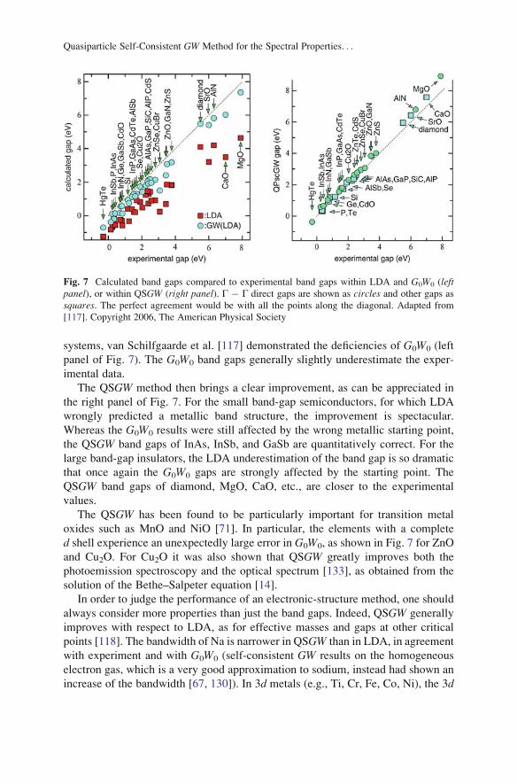
systems, van Schilfgaarde et al. [117] demonstrated the deficiencies of G0W0 (left

panel of Fig. 7). The G0W0 band gaps generally slightly underestimate the exper-

imental data.

The QSGW method then brings a clear improvement, as can be appreciated in

the right panel of Fig. 7. For the small band-gap semiconductors, for which LDA

wrongly predicted a metallic band structure, the improvement is spectacular.

Whereas the G0W0 results were still affected by the wrong metallic starting point,

the QSGW band gaps of InAs, InSb, and GaSb are quantitatively correct. For the

large band-gap insulators, the LDA underestimation of the band gap is so dramatic

that once again the G0W0 gaps are strongly affected by the starting point. The

QSGW band gaps of diamond, MgO, CaO, etc., are closer to the experimental

values.

The QSGW has been found to be particularly important for transition metal

oxides such as MnO and NiO [71]. In particular, the elements with a complete

d shell experience an unexpectedly large error in G0W0, as shown in Fig. 7 for ZnO

and Cu2O. For Cu2O it was also shown that QSGW greatly improves both the

photoemission spectroscopy and the optical spectrum [133], as obtained from the

solution of the Bethe–Salpeter equation [14].

In order to judge the performance of an electronic-structure method, one should

always consider more properties than just the band gaps. Indeed, QSGW generally

improves with respect to LDA, as for effective masses and gaps at other critical

points [118]. The bandwidth of Na is narrower in QSGW than in LDA, in agreement

with experiment and with G0W0 (self-consistent GW results on the homogeneous

electron gas, which is a very good approximation to sodium, instead had shown an

increase of the bandwidth [67, 130]). In 3d metals (e.g., Ti, Cr, Fe, Co, Ni), the 3d

Fig. 7 Calculated band gaps compared to experimental band gaps within LDA and G0W0 (leftpanel), or within QSGW (right panel). Γ � Γ direct gaps are shown as circles and other gaps as

squares. The perfect agreement would be with all the points along the diagonal. Adapted from

[117]. Copyright 2006, The American Physical Society


bandwidths, the exchange splittings, and magnetic moments are generally

improved with respect to LDA [117], with some exceptions like Ni and other

systems where LDA already overestimates the magnetic moment, and one expects

that the coupling with spin fluctuations beyond GW should be taken into account

[57]. In addition to spectroscopic data, some ground-state properties can also be

successfully predicted with QSGW, such as electric field gradients [134]. Finally,

QSGW results have also been used as a starting point for other calculations, like

impact ionization rates [135] and the transverse spin susceptibility [136], again

finding good agreement with experiment.

There is still an overall slight overestimation of the band gaps by the QSGWmethod, which is systematic in all compounds studied [117, 118]. The accuracy of

QSGW somewhat deteriorates in d and f compounds with respect to sp systems. The

unoccupied states are generally too high: by 0.2 eV for sp semiconductors, less than

1 eV for d0 compounds like SrTiO3 and TiO2, more than 1 eV for other d materials

like NiO, and up to 3 eV for f compounds like Gd and Er [119]. Most often these

errors have been ascribed to the missing electron–hole interactions (excitonic

effects) in the calculation of the polarization eχ and the screened interaction

W, which is done at the RPA level in the GW approximation. The dielectric

constants turn out to be too small (by ~20%) [117], resulting in a slight

underscreening and, in turn, into too large gaps. Indeed, van Schilfgaarde and

coworkers empirically found that by rescaling by 0.8 the screened interaction

W, the results were improved (see, e.g., [123, 124, 137]). This tendency was later

confirmed by Shishkin et al. [138], who corrected the remaining error with the

inclusion of electron-hole interaction in W using the Nanoquanta kernel of time-

dependent density-functional theory [139]. These observations mean that vertex

corrections in Σ – see (13f)] – would play a secondary role in a large variety of

materials. However, for example, the localized d band in the occupied valence bandof materials like GaAs, GaN, and GaP, which is slightly too shallow, cannot be

corrected by this simple rescaling that corrects the QSGW underscreening. A more

detailed investigation of the effects of vertex corrections beyond GW is thus still an

open issue.

Of course, not all the features of the full GW self-energy can be retained in

QSGW. The simplicity has a price. Being a quasiparticle-only theory, all the

properties beyond quasiparticles are naturally absent in QSGW. For instance, the

satellites in the photoemission spectra of correlated [57] and non-correlated [56]

materials are no longer accessible. The finite lifetimes of quasiparticles [58] are also

beyond QSGW. A way to overcome this limitation is to use the QSGW results at

self-consistency as a starting point to calculate the Green’s function in the GWapproximation and hence the spectral function, as has been done recently for

SrVO3 [107].

The QSGW has mostly been applied to solids. Nowadays, the first applications to

atoms and molecules are being carried out by several groups. Bruneval [34] first

applied QSGW to the ionization potential of small sodium clusters. Then Ke [140]

demonstrated the improvement of QSGW compared to G0W0 based on Hartree–

Fock for the conjugated molecules (CnHm) for electron affinities and ionization


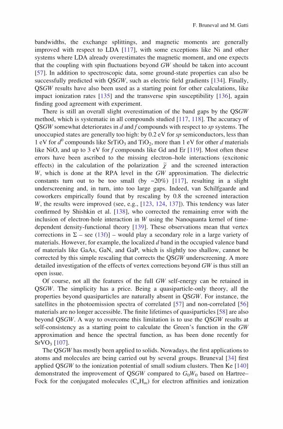
potentials. More recently, Bruneval [141] investigated its performance for all the

light atoms from H to Ar. As shown in Fig. 8, the improvement offered by QSGW is

not systematic. On average QSGW performs better than G0W0 based on HF with a

relatively smaller mean absolute error, although for specific atoms the opposite can

hold true. Note that the error in the LUMO of the positive ion (right panel) remains

rather large even for QSGW. Of course, the application of QSGW to molecules is

still in its early stage and its performance has to be evaluated for a wider range of

molecules, especially for large molecules.

5 Relation with Alternative Self-Consistent Schemes

Although the QSGW method is a simplified version of the full self-consistent GWself-energy, the calculations may still be quite cumbersome. Many authors resort to

even more approximated types of self-consistency. This section briefly describes

the alternatives to QSGW.

5.1 Energy-Only Self-Consistency

In the energy-only self-consistent GW scheme, the eigenvalues used to build G and

W are updated iteratively, while the wavefunctions are kept at the level of the mean-

field starting point. This scheme corresponds to keeping only the diagonal terms of

the QSGW Hamiltonian. Thus whenever the mean-field orbitals are a good approx-

imation to QP wavefunctions, the two schemes will give very similar results. Of

H He Li Be B C N O F Ne Na Mg Al Si P S Cl Ar

-1.0

-0.9

-0.8

-0.7

-0.6

-0.5

-0.4

-0.3

-0.2

-0.1

0.0

0.1

0.2

0.3

0.4

0.5

0.6

0.7

Err

or w

rt E

xpt.

(eV

)

HF MAE = 0.46 eVGW@HF MAE = 0.27 eVQSGW MAE = 0.18 eV

H+

He+

Li+

Be+

B+

C+

N+

O+

F+

Ne+

Na+

Mg+

Al+

Si+

P+

S+

Cl+

Ar+

-0.4

-0.3

-0.2

-0.1

0.0

0.1

0.2

0.3

0.4

0.5

0.6

0.7

0.8

0.9

1.0

1.1

1.2

1.3

Err

or w

rt E

xpt.

(eV

)

HF MAE = 1.74 eVGW@HF MAE = 0.43 eVQSGW MAE = 0.34 eV

Fig. 8 Deviation from the experimental ionization potential of atoms as obtained from the HOMO

of the neutral atoms (left panel) or from the LUMO of the positive ions (right panel), i.e., EHOMO/

LUMO � (�I ). HF is presented with open bars, G0W0 based on HF inputs (GW@HF) with stripedbars, and QSGW with filled bars. The mean absolute error (MAE) is also provided. Reprinted with

permission from [141]. Copyright 2012, American Institute of Physics


course, the energy-only self-consistent GW is computationally much cheaper than

QSGW.

This scheme has been used many times in the past [83, 142–145] in order to

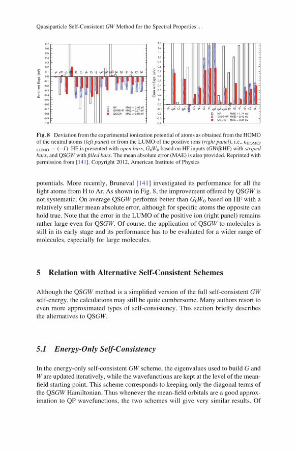
improve band gaps and band widths with respect to G0W0 results. Recently,

Shishkin and Kresse [145] presented a systematic study of the band gap of several

sp semiconductors and insulators. The conclusion of their analysis is that updating

the eigenvalues in G while keepingW at the GGA level (the scheme is called GW0)

gives the best results in comparison to experiment (see Fig. 9). This is due to a

cancellation of effects between the band-gap opening and excitonic interactions in

W that is verified in the class of materials considered in [145]. In turn, the GGA

screening is in better agreement with the physical one (i.e., the one that can be

measured by loss spectroscopies) than the screening calculated self-consistently. In

fact, updating the eigenvalues in W also leads to an underscreening and further

opens the gaps, causing the results to deteriorate [145]. Similar conclusions can be

reached in finite systems. For instance, Blase and coworkers [94, 146] recently

found that in a set of organic molecules and DNA/RNA nucleobases the energy-

only self-consistent GW scheme provides much better results than G0W0 on top of

LDA.

5.2 Alternatives to the QSGW: COHSEX and Others

COHSEX is a static and Hermitian approximation to the GW self-energy (see

Sect. 2.4). In this respect it parallels the self-energy of the QSGW approximation.

Fig. 9 Comparison of band

gaps calculated in GGA

(PBE), G0W0, and GW0,

with experiment for a series

of prototypical spsemiconductors and

insulators. GW0 performs

best. From [145]. Copyright

2007, The American

Physical Society


The difference between the two approximations is the fact that in COHSEX the

screening is static (i.e., it is calculated only at ω ¼ 0), while it is fully dynamical in

QSGW.

Bruneval, Vast, and Reining [112] proposed to combine self-consistent

COHSEX with a subsequent G0W0 calculation, giving very similar results to

QSGW [112, 133] at a much lower computational cost. In fact, in COHSEX both

the calculations of the screening (only static) and the self-energy (depending only

on occupied states) are cheaper than in GW. COHSEX alone generally overesti-

mates band gaps and dynamical effects contained in the GW self-energy are needed

to correct this overestimation. In many cases a perturbative G0W0 correction is

sufficient, while, for example, in prototypical transition metal oxides like NiO and

MnO, a self-consistent update of the eigenvalues is needed to get results similar to

QSGW [147, Gatti and Rubio (2013) Unpublished].

The COHSEX+ G0W0 scheme has been successfully applied in a wide range of

materials: from transition metal compounds (e.g., Cu2O, VO2, NiS2�xSex [105, 126,

133]) to CIGS and quaternary chalcogenides [120, 125, 148], delafossite transpar-

ent conductive oxides [121, 149], and intermediate-band materials [150, 151].

In an earlier work, Gygi and Baldereschi derived a simplified model static self-

energy from the GW approximation [152] that was later used in a self-consistent

manner in several transition metal oxides (e.g., MnO, NiO, CaCuO2, and VO2

[153–155]). These applications employed a model screened interactionW in which

the static dielectric constant was a parameter taken from experiment. Nevertheless,

together with the work of Aryasetiawan and Gunnarsson on NiO [156], in which the

self-consistency was simulated by adding to LDA a static correction term for the

Ni eg bands, they provided the first meaningful GW descriptions of these transition

metal oxides beyond the G0W0 scheme.

More recently, Sakuma, Miyake, and Aryasetiawan have proposed an alternative

self-consistent quasiparticle scheme that is based on Lowdin’s method of symmet-

ric orthogonalization [157]. Results have been found to be very close to those in the

QSGW scheme.

5.3 Hybrid Functionals and LDA+U

Hybrid functionals [158] and the LDA+U approach [159] have become very

popular as improved exchange-correlation DFT functionals in solids. At the same

time, both can be seen as an approximation to the GW self-energy [160, 161]. In

hybrids like the Heyd–Scuseria–Ernzerhof (HSE) functional [158] the α and

ω parameters, which are obtained by considerations of the adiabatic-connection

formula and numerically fitting the results against a benchmark set of data, play the

role of effective screening. In LDA+U the on-site Hubbard U correction is only

applied to a subset of states (and a double-counting correction is introduced). The

electron–electron local interaction is treated at the Hartree–Fock level and the

screening of the interaction is effectively obtained by reducing U from its atomic


values. The Hubbard U can be pragmatically used as fitting parameter or calculated

for example in RPA: in this case all the electrons not belonging to the chosen subset

of states are then providing the effective screening of U [162]. The common effect

of both hybrid functionals and LDA+U is to produce, as a result of an exchange

effect, a localization of the LDA orbitals that for d and f electrons are generally toodelocalized.

Even though both methods depend on parameters, they can be seen as a cheap

way to perform self-consistent quasiparticle calculations. In fact, in recent years

they have been proposed as an improved starting point for subsequent G0W0

calculations. In particular, Rodl and coworkers [163–165] have shown that in

prototypical transition metal oxides it is possible to fit the more expensive HSE

results from GGA+U calculations with an additional scissor shift, producing results

in good agreement with experiments. The application of these computationally

efficient schemes is also gaining quite a large popularity in theGW community (see,

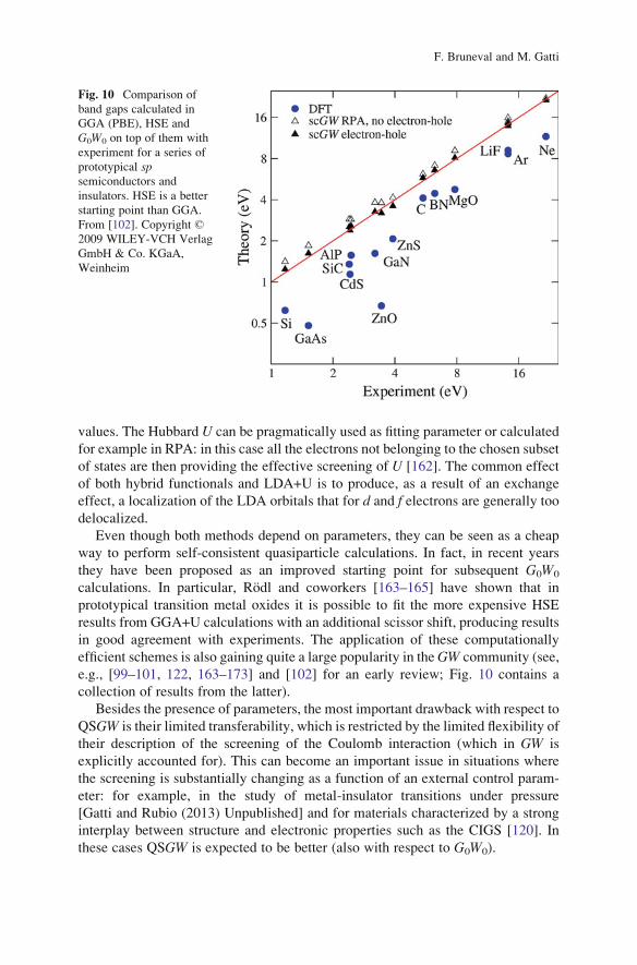
e.g., [99–101, 122, 163–173] and [102] for an early review; Fig. 10 contains a

collection of results from the latter).

Besides the presence of parameters, the most important drawback with respect to

QSGW is their limited transferability, which is restricted by the limited flexibility of

their description of the screening of the Coulomb interaction (which in GW is

explicitly accounted for). This can become an important issue in situations where

the screening is substantially changing as a function of an external control param-

eter: for example, in the study of metal-insulator transitions under pressure

[Gatti and Rubio (2013) Unpublished] and for materials characterized by a strong

interplay between structure and electronic properties such as the CIGS [120]. In

these cases QSGW is expected to be better (also with respect to G0W0).

Fig. 10 Comparison of

band gaps calculated in

GGA (PBE), HSE and

G0W0 on top of them with

experiment for a series of

prototypical spsemiconductors and

insulators. HSE is a better

starting point than GGA.

From [102]. Copyright ©2009 WILEY-VCH Verlag

GmbH & Co. KGaA,

Weinheim


6 Conclusions and Outlook

The present chapter aimed at presenting the robustness and the simplicity of the

QSGW when addressing the spectral properties of materials. The QSGW method is

nowadays a mature theory that offers a remarkable trade-off between speed and

accuracy.

It has been applied to an impressively wide variety of materials, covering the

range from sodium [113] to uranium and plutonium [174, 175], and including

metals, semi-conductors, insulators, atoms, and molecules. The comparison to

experiment is in general very favorable. Therefore, in our opinion, QSGW is, to

date, the best ab initio method available to calculate the quasiparticle spectrum of

photoemission (and inverse photoemission) for solid state systems and can be

thought of as a predictive theory.

Furthermore, QSGW is readily available in popular codes, such as Abinit [176]

or Vasp [177]. On the other hand, the increasing popularity of the method nowadays

goes hand in hand with the need for optimizing the computational algorithms, in

order to prevent slow convergence in the self-consistency (see, e.g., [178]).

The QSGW method has enlarged the range of compounds that can be described

by the GW approximation. It has demonstrated that, for materials for which G0W0

was performing badly and thus considered out of reach for ab initio methods

(e.g. “strongly correlated” transition metal oxides), the failure was to be ascribed

to the perturbative scheme of G0W0, and not to the GW approximation itself [71].

QSGW has provided an accurate reference from which it now makes sense to

investigate more refined features of the electronic structure of materials, such as

electron–phonon coupling [61, 62] and lattice polarization [179], which now are

larger than the error bar of the method. Analogously, the field is now ready to study

effects of electron interaction beyond the GW approximation (i.e., vertex correc-

tions, for example, through the coupling with other approximations), without the

bias that the perturbative G0W0 scheme introduces.

Acknowledgments We thank Mark van Schilfgaarde for a critical reading of the chapter.

References

1. Hufner S (2010) Photoelectron spectroscopy, 3rd edn. Springer, Berlin

2. Damascelli A, Hussain Z, Shen ZX (2003) Rev Mod Phys 75:473. doi:10.1103/RevModPhys.

75.473

3. Bardyszewski W, Hedin L (1985) Phys Scripta 32(4):439

4. Hedin L, Michiels J, Inglesfield J (1998) Phys Rev B 58:15565. doi:10.1103/PhysRevB.58.

15565

5. Hedin L (1999) J Phys Condens Matter 11(42):R489

6. Braun J (1996) Rep Prog Phys 59(10):1267

7. Minar J, Braun J, Mankovsky S, Ebert H (2011) advances in vacuum ultraviolet and X-ray

physics: the 37th international conference on vacuum ultraviolet and X-ray physics


http://dx.doi.org/10.1103/RevModPhys.75.473


http://dx.doi.org/10.1103/PhysRevB.58.15565


(VUVX2010). J Electron Spectros Relat Phenomena 184(36):91. doi:10.1016/j.elspec.2011.

01.009

8. Minar J, Braun J, Ebert H (2012) J Electron Spectrosc Relat Phenomena (0). doi:10.1016/j.

elspec.2012.10.003

9. Papalazarou E, Gatti M, Marsi M, Brouet V, Iori F, Reining L, Annese E, Vobornik I, Offi F,

Fondacaro A, Huotari S, Lacovig P, Tjernberg O, Brookes NB, Sacchi M, Metcalf P,

Panaccione G (2009) Phys Rev B 80:155115. doi:10.1103/PhysRevB.80.155115

10. Hohenberg P, Kohn W (1964) Phys Rev 136(3B):B864. doi:10.1103/PhysRev.136.B864

11. Kohn W, Sham LJ (1965) Phys Rev 140:A1133. doi:10.1103/PhysRev.140.A1133

12. Sham LJ, Kohn W (1966) Phys Rev 145:561. doi:10.1103/PhysRev.145.561

13. Janak JF (1978) Phys Rev B 18:7165. doi:10.1103/PhysRevB.18.7165

14. Onida G, Reining L, Rubio A (2002) Rev Mod Phys 74:601. doi:10.1103/RevModPhys.74.

601

15. Godby RW, White ID (1998) Phys Rev Lett 80:3161. doi:10.1103/PhysRevLett.80.3161

16. Sham LJ, Schluter M (1983) Phys Rev Lett 51:1888. doi:10.1103/PhysRevLett.51.1888

17. Perdew JP, Levy M (1983) Phys Rev Lett 51:1884. doi:10.1103/PhysRevLett.51.1884

18. Godby RW, Schluter M, Sham LJ (1986) Phys Rev Lett 56:2415. doi:10.1103/PhysRevLett.

56.2415

19. Holzmann M, Bernu B, Pierleoni C, McMinis J, Ceperley DM, Olevano V, Delle Site L

(2011) Phys Rev Lett 107:110402. doi:10.1103/PhysRevLett.107.110402

20. Gatti M, Olevano V, Reining L, Tokatly IV (2007) Phys Rev Lett 99:057401. doi:10.1103/

PhysRevLett.99.057401

21. Booth GH, Gruneis A, Kresse G, Alavi A (2013) Nature 493(7432):365

22. Fetter AL, Walecka JD (1971) Quantum theory of many-particle systems. MacGraw-Hill,

New York

23. Mahan GD (1981) Many-particle physics. Plenum, New York

24. Gross EKU, Runge E, Heinonen O (1991) Many-particle theory. Adam Hilger, Bristol

25. Hedin L (1965) Phys Rev 139:A796. doi:10.1103/PhysRev.139.A796

26. Hedin L, Lundqvist S (1970) Academic, pp 1–181. doi:10.1016/S0081-1947(08)60615-3

27. Aryasetiawan F, Gunnarsson O (1998) Rep Prog Phys 61(3):237

28. Aulbur WG, Jonsson L, Wilkins JW (1999) Academic, pp 1–218. doi:10.1016/S0081-

1947(08)60248-9

29. Shaltaf R, Rignanese GM, Gonze X, Giustino F, Pasquarello A (2008) Phys Rev Lett

100:186401. doi:10.1103/PhysRevLett.100.186401

30. Wang NP, Rohlfing M, Kruger P, Pollmann J (2005) Phys Rev B 71:045407. doi:10.1103/

PhysRevB.71.045407

31. Thygesen KS, Rubio A (2009) Phys Rev Lett 102:046802. doi:10.1103/PhysRevLett.102.

046802

32. Garcia-Lastra JM, Rostgaard C, Rubio A, Thygesen KS (2009) Phys Rev B 80:245427.

doi:10.1103/PhysRevB.80.245427

33. Rinke P, Janotti A, Scheffler M, Van de Walle CG (2009) Phys Rev Lett 102:026402. doi:10.

1103/PhysRevLett.102.026402

34. Bruneval F (2009) Phys Rev Lett 103:176403. doi:10.1103/PhysRevLett.103.176403

35. Bockstedte M, Marini A, Pankratov O, Rubio A (2010) Phys Rev Lett 105:026401. doi:10.


36. Ma Y, Rohlfing M, Gali A (2010) Phys Rev B 81:041204. doi:10.1103/PhysRevB.81.041204

37. Jain M, Chelikowsky JR, Louie SG (2011) Phys Rev Lett 107:216803. doi:10.1103/


38. Bruneval F, Roma G (2011) Phys Rev B 83:144116. doi:10.1103/PhysRevB.83.144116

39. Neaton JB, Hybertsen MS, Louie SG (2006) Phys Rev Lett 97:216405. doi:10.1103/


40. Darancet P, Ferretti A, Mayou D, Olevano V (2007) Phys Rev B 75:075102. doi:10.1103/

PhysRevB.75.075102


http://dx.doi.org/10.1016/j.elspec.2011.01.009





http://dx.doi.org/10.1103/PhysRev.136.B864

http://dx.doi.org/10.1103/PhysRev.140.A1133

http://dx.doi.org/10.1103/PhysRev.145.561




http://dx.doi.org/10.1103/PhysRevLett.80.3161








http://dx.doi.org/10.1103/PhysRev.139.A796

http://dx.doi.org/10.1016/S0081-1947(08)60615-3

http://dx.doi.org/10.1016/S0081-1947(08)60248-9

http://dx.doi.org/10.1016/S0081-1947(08)60248-9




















41. Thygesen KS, Rubio A (2008) Phys Rev B 77:115333. doi:10.1103/PhysRevB.77.115333

42. Myohanen P, Stan A, Stefanucci G, van Leeuwen R (2009) Phys Rev B 80:115107. doi:10.

1103/PhysRevB.80.115107

43. Rangel T, Ferretti A, Trevisanutto PE, Olevano V, Rignanese GM (2011) Phys Rev B

84:045426. doi:10.1103/PhysRevB.84.045426

44. Reining L, Onida G, Godby RW (1997) Phys Rev B 56:R4301. doi:10.1103/PhysRevB.56.

R4301

45. Bruneval F, Gonze X (2008) Phys Rev B 78:085125. doi:10.1103/PhysRevB.78.085125

46. Umari P, Stenuit G, Baroni S (2010) Phys Rev B 81:115104. doi:10.1103/PhysRevB.81.

115104

47. Giustino F, Cohen ML, Louie SG (2010) Phys Rev B 81:115105. doi:10.1103/PhysRevB.81.

115105

48. Berger JA, Reining L, Sottile F (2010) Phys Rev B 82:041103. doi:10.1103/PhysRevB.82.

041103

49. Nguyen HV, Pham TA, Rocca D, Galli G (2012) Phys Rev B 85:081101. doi:10.1103/

PhysRevB.85.081101

50. Bruneval F, Sottile F, Olevano V, Del Sole R, Reining L (2005) Phys Rev Lett 94:186402.

doi:10.1103/PhysRevLett.94.186402. URL

51. Nelson W, Bokes P, Rinke P, Godby RW (2007) Phys Rev A 75:032505. doi:10.1103/

PhysRevA.75.032505

52. Morris AJ, Stankovski M, Delaney KT, Rinke P, Garcıa-Gonzalez P, Godby RW (2007) Phys

Rev B 76:155106. doi:10.1103/PhysRevB.76.155106

53. Romaniello P, Guyot S, Reining L (2009) J Chem Phys 131(15):154111. doi:10.1063/1.

3249965

54. Caruso F, Rohr DR, Hellgren M, Ren X, Rinke P, Rubio A, Scheffler M (2013) Phys Rev Lett

110:146403. doi:10.1103/PhysRevLett.110.146403

55. Aryasetiawan F, Hedin L, Karlsson K (1996) Phys Rev Lett 77:2268. doi:10.1103/

PhysRevLett.77.2268

56. Guzzo M, Lani G, Sottile F, Romaniello P, Gatti M, Kas JJ, Rehr JJ, Silly MG, Sirotti F,

Reining L (2011) Phys Rev Lett 107:166401. doi:10.1103/PhysRevLett.107.166401

57. Springer M, Aryasetiawan F, Karlsson K (1998) Phys Rev Lett 80:2389. doi:10.1103/

PhysRevLett.80.2389

58. Zhukov VP, Chulkov EV, Echenique PM (2004) Phys Rev Lett 93:096401. doi:10.1103/


59. Romaniello P, Bechstedt F, Reining L (2012) Phys Rev B 85:155131. doi:10.1103/

PhysRevB.85.155131

60. Biermann S, Aryasetiawan F, Georges A (2003) Phys Rev Lett 90:086402. doi:10.1103/


61. Giustino F, Louie SG, Cohen ML (2010) Phys Rev Lett 105:265501. doi:10.1103/


62. Cannuccia E, Marini A (2011) Phys Rev Lett 107:255501. doi:10.1103/PhysRevLett.107.

255501

63. Dahlen NE, van Leeuwen R (2007) Phys Rev Lett 98:153004. doi:10.1103/PhysRevLett.98.

153004

64. von Friesen MP, Verdozzi C, Almbladh CO (2009) Phys Rev Lett 103:176404. doi:10.1103/


65. Puig von Friesen M, Verdozzi C, Almbladh CO (2010) Phys Rev B 82:155108. doi:10.1103/

PhysRevB.82.155108

66. Schindlmayr A, Pollehn TJ, Godby RW (1998) Phys Rev B 58:12684. doi:10.1103/

PhysRevB.58.12684

67. Holm B, von Barth U (1998) Phys Rev B 57:2108. doi:10.1103/PhysRevB.57.2108

68. Holm B (1999) Phys Rev Lett 83:788. doi:10.1103/PhysRevLett.83.788






http://dx.doi.org/10.1103/PhysRevB.56.R4301

http://dx.doi.org/10.1103/PhysRevB.56.R4301










http://dx.doi.org/10.1103/PhysRevLett.94.186402.%20URL

http://dx.doi.org/10.1103/PhysRevA.75.032505

http://dx.doi.org/10.1103/PhysRevA.75.032505


http://dx.doi.org/10.1063/1.3249965

http://dx.doi.org/10.1063/1.3249965



























69. Garcıa-Gonzalez P, Godby RW (2001) Phys Rev B 63:075112. doi:10.1103/PhysRevB.63.

075112

70. Ismail-Beigi S (2010) Phys Rev B 81:195126. doi:10.1103/PhysRevB.81.195126

71. Faleev SV, van Schilfgaarde M, Kotani T (2004) Phys Rev Lett 93:126406. doi:10.1103/


72. Strinati G (1988) Rivista del Nuovo Cimento 11:1

73. Møller C, Plesset MS (1934) Phys Rev 46:618. doi:10.1103/PhysRev.46.618

74. Adler SL (1963) Phys Rev 130:1654. doi:10.1103/PhysRev.130.1654

75. Wiser N (1963) Phys Rev 129:62. doi:10.1103/PhysRev.129.62

76. Strinati G, Mattausch HJ, Hanke W (1980) Phys Rev Lett 45:290. doi:10.1103/PhysRevLett.

45.290

77. Hybertsen MS, Louie SG (1985) Phys Rev Lett 55:1418. doi:10.1103/PhysRevLett.55.1418

78. Shirley EL, Martin RM (1993) Phys Rev B 47:15404. doi:10.1103/PhysRevB.47.15404

79. Hedin L, Lundqvist B, Lundqvist S (1967) Solid State Commun 5(4):237. doi:10.1016/0038-

1098(67)90264-5

80. Lundqvist B (1967) Physik der kondensierten Materie 6(3):193. doi:10.1007/BF02422716

81. Blomberg C, Bergersen B (1972) Can J Phys 50(19):2286. doi:10.1139/p72-303

82. Bergersen B, Kus FW, Blomberg C (1973) Can J Phys 51(1):102. doi:10.1139/p73-012

83. Hybertsen MS, Louie SG (1986) Phys Rev B 34:5390. doi:10.1103/PhysRevB.34.5390

84. Godby RW, Needs RJ (1989) Phys Rev Lett 62(10):1169. doi:10.1103/PhysRevLett.62.1169

85. Lebegue S, Arnaud B, Alouani M, Bloechl PE (2003) Phys Rev B 67(15):155208. doi:10.

1103/PhysRevB.67.155208

86. Morin FJ (1959) Phys Rev Lett 3(1):34. doi:10.1103/PhysRevLett.3.34

87. Del Sole R, Reining L, Godby RW (1994) Phys Rev B 49:8024. doi:10.1103/PhysRevB.49.

8024

88. Cazzaniga M (2012) Phys Rev B 86:035120. doi:10.1103/PhysRevB.86.035120

89. Marini A, Rubio A (2004) Phys Rev B 70:081103. doi:10.1103/PhysRevB.70.081103

90. Stankovski M (2008) Local and non-local vertex corrections beyond the GW approximation.

Ph.D. thesis, University of York

91. Rostgaard C, Jacobsen KW, Thygesen KS (2010) Phys Rev B 81:085103. doi:10.1103/

PhysRevB.81.085103

92. Bruneval F, Marques MAL (2013) J Chem Theory Comput 9(1):324. doi:10.1021/ct300835h

93. Stan A, Dahlen NE, van Leeuwen R (2006) Europhys Lett 76(2):298

94. Blase X, Attaccalite C, Olevano V (2011) Phys Rev B 83:115103. doi:10.1103/PhysRevB.83.

115103

95. Caruso F, Rinke P, Ren X, Scheffler M, Rubio A (2012) Phys Rev B 86:081102. doi:10.1103/

PhysRevB.86.081102

96. Marom N, Caruso F, Ren X, Hofmann OT, Korzdorfer T, Chelikowsky JR, Rubio A,

Scheffler M, Rinke P (2012) Phys Rev B 86:245127. doi:10.1103/PhysRevB.86.245127

97. Rinke P, Qteish A, Neugebauer J, Freysoldt C, Scheffler M (2005) New J Phys 7(1):126

98. Rinke P, Qteish A, Neugebauer J, Scheffler M (2008) Phys Status Solidi B 245(5):929.

doi:10.1002/pssb.200743380

99. Miyake T, Zhang P, Cohen ML, Louie SG (2006) Phys Rev B 74:245213. doi:10.1103/

PhysRevB.74.245213

100. Jiang H, Gomez-Abal RI, Rinke P, Scheffler M (2009) Phys Rev Lett 102:126403. doi:10.


101. Fuchs F, Furthmuller J, Bechstedt F, Shishkin M, Kresse G (2007) Phys Rev B 76:115109.

doi:10.1103/PhysRevB.76.115109

102. Bechstedt F, Fuchs F, Kresse G (2009) Phys Status Solidi B 246(8):1877. doi:10.1002/pssb.

200945074

103. Koethe TC, Hu Z, Haverkort MW, Schußler-Langeheine C, Venturini F, Brookes NB,

Tjernberg O, Reichelt W, Hsieh HH, Lin HJ, Chen CT, Tjeng LH (2006) Phys Rev Lett

97:116402. doi:10.1103/PhysRevLett.97.116402














http://dx.doi.org/10.1016/0038-1098(67)90264-5

http://dx.doi.org/10.1016/0038-1098(67)90264-5

http://dx.doi.org/10.1007/BF02422716

http://dx.doi.org/10.1139/p72-303

http://dx.doi.org/10.1139/p73-012












http://dx.doi.org/10.1021/ct300835h






http://dx.doi.org/10.1002/pssb.200743380









104. Sakuma R, Miyake T, Aryasetiawan F (2008) Phys Rev B 78:075106. doi:10.1103/

PhysRevB.78.075106

105. Gatti M, Bruneval F, Olevano V, Reining L (2007) Phys Rev Lett 99:266402. doi:10.1103/


106. Pollehn TJ, Schindlmayr A, Godby RW (1998) J Phys Condens Matter 10(6):1273

107. Gatti M, Guzzo M (2013) Phys Rev B 87:155147. doi:10.1103/PhysRevB.87.155147

108. Rohlfing M, Louie SG (2000) Phys Rev B 62:4927. doi:10.1103/PhysRevB.62.4927

109. White ID, Godby RW, Rieger MM, Needs RJ (1998) Phys Rev Lett 80:4265. doi:10.1103/

PhysRevLett.80.4265

110. Pulci O, Bechstedt F, Onida G, Del Sole R, Reining L (1999) Phys Rev B 60:16758. doi:10.

1103/PhysRevB.60.16758

111. Rohlfing M, Wang NP, Kruger P, Pollmann J (2003) Phys Rev Lett 91:256802. doi:10.1103/


112. Bruneval F, Vast N, Reining L (2006) Phys Rev B 74:045102. doi:10.1103/PhysRevB.74.

045102

113. van Schilfgaarde M, Kotani T, Faleev SV (2006) Phys Rev B 74:245125. doi:10.1103/

PhysRevB.74.245125

114. Marsili M, Pulci O, Bechstedt F, Del Sole R (2005) Phys Rev B 72:115415. doi:10.1103/

PhysRevB.72.115415

115. Wentzcovitch RM, Schulz WW, Allen PB (1994) Phys Rev Lett 72:3389. doi:10.1103/

PhysRevLett.72.3389

116. Zylbersztejn A, Mott NF (1975) Phys Rev B 11:4383. doi:10.1103/PhysRevB.11.4383

117. van Schilfgaarde M, Kotani T, Faleev S (2006) Phys Rev Lett 96:226402. doi:10.1103/


118. Kotani T, van Schilfgaarde M, Faleev SV (2007) Phys Rev B 76:165106. doi:10.1103/

PhysRevB.76.165106

119. Chantis AN, van Schilfgaarde M, Kotani T (2007) Phys Rev B 76:165126. doi:10.1103/

PhysRevB.76.165126

120. Vidal J, Botti S, Olsson P, Guillemoles JF, Reining L (2010) Phys Rev Lett 104:056401

121. Vidal J, Trani F, Bruneval F, Marques MAL, Botti S (2010) Phys Rev Lett 104:136401.

doi:10.1103/PhysRevLett.104.136401

122. Franchini C, Sanna A, Marsman M, Kresse G (2010) Phys Rev B 81:085213. doi:10.1103/

PhysRevB.81.085213

123. Svane A, Christensen NE, Cardona M, Chantis AN, van Schilfgaarde M, Kotani T (2010)

Phys Rev B 81:245120. doi:10.1103/PhysRevB.81.245120

124. Svane A, Christensen NE, Cardona M, Chantis AN, van Schilfgaarde M, Kotani T (2011)

Phys Rev B 84:205205. doi:10.1103/PhysRevB.84.205205

125. Aguilera I, Vidal J, Wahnon P, Reining L, Botti S (2011) Phys Rev B 84:085145. doi:10.

1103/PhysRevB.84.085145

126. Schuster C, Gatti M, Rubio A (2012) Eur Phys J B 85:1. doi:10.1140/epjb/e2012-30384-7

127. Baroni S, Resta R (1986) Phys Rev B 33(10):7017. doi:10.1103/PhysRevB.33.7017

128. Baym G, Kadanoff LP (1961) Phys Rev 124:287. doi:10.1103/PhysRev.124.287

129. Schindlmayr A, Garcıa-Gonzalez P, Godby RW (2001) Phys Rev B 64:235106. doi:10.1103/

PhysRevB.64.235106

130. Shirley EL (1996) Phys Rev B 54:7758. doi:10.1103/PhysRevB.54.7758

131. Bechstedt F, Tenelsen K, Adolph B, Del Sole R (1997) Phys Rev Lett 78:1528. doi:10.1103/

PhysRevLett.78.1528

132. Stan A, Dahlen NE, van Leeuwen R (2009) J Chem Phys 130(11):114105. doi:10.1063/1.

3089567

133. Bruneval F, Vast N, Reining L, Izquierdo M, Sirotti F, Barrett N (2006) Phys Rev Lett

97:267601. doi:10.1103/PhysRevLett.97.267601

134. Christensen NE, Svane A, Laskowski R, Palanivel B, Modak P, Chantis AN, van

Schilfgaarde M, Kotani T (2010) Phys Rev B 81:045203. doi:10.1103/PhysRevB.81.045203




































http://dx.doi.org/10.1140/epjb/e2012-30384-7








http://dx.doi.org/10.1063/1.3089567

http://dx.doi.org/10.1063/1.3089567



135. Kotani T, van Schilfgaarde M (2010) Phys Rev B 81:125201. doi:10.1103/PhysRevB.81.

125201

136. Kotani T, van Schilfgaarde M (2008) J Phys Condens Matter 20(29):295214

137. Punya A, Lambrecht WRL, van Schilfgaarde M (2011) Phys Rev B 84:165204. doi:10.1103/

PhysRevB.84.165204

138. Shishkin M, Marsman M, Kresse G (2007) Phys Rev Lett 99:246403. doi:10.1103/


139. Botti S, Schindlmayr A, Sole RD, Reining L (2007) Rep Prog Phys 70(3):357

140. Ke SH (2011) Phys Rev B 84:205415. doi:10.1103/PhysRevB.84.205415

141. Bruneval F (2012) J Chem Phys 136(19):194107. doi:10.1063/1.4718428

142. Northrup JE, Hybertsen MS, Louie SG (1987) Phys Rev Lett 59:819. doi:10.1103/

PhysRevLett.59.819

143. Luo W, Ismail-Beigi S, Cohen ML, Louie SG (2002) Phys Rev B 66:195215. doi:10.1103/

PhysRevB.66.195215

144. Fleszar A, Hanke W (2005) Phys Rev B 71:045207. doi:10.1103/PhysRevB.71.045207

145. Shishkin M, Kresse G (2007) Phys Rev B 75:235102. doi:10.1103/PhysRevB.75.235102

146. Faber C, Attaccalite C, Olevano V, Runge E, Blase X (2011) Phys Rev B 83:115123. doi:10.

1103/PhysRevB.83.115123

147. Guzzo M (2008) Exchange and correlation effects in the electronic properties of transition

metal oxides: the example of NiO. Master’s thesis, Universita degli studi di Milano-Bicocca

148. Botti S, Kammerlander D, Marques MAL (2011) Appl Phys Lett, 98(24). doi: 10.1063/

1.3600060

149. Trani F, Vidal J, Botti S, Marques MAL (2010) Phys Rev B 82:085115. doi:10.1103/

PhysRevB.82.085115

150. Aguilera I, Palacios P, Wahnon P (2011) Phys Rev B 84:115106. doi:10.1103/PhysRevB.84.

115106

151. Lucero MJ, Aguilera I, Diaconu CV, Palacios P, Wahnon P, Scuseria GE (2011) Phys Rev B

83:205128. doi:10.1103/PhysRevB.83.205128

152. Gygi F, Baldereschi A (1989) Phys Rev Lett 62:2160. doi:10.1103/PhysRevLett.62.2160

153. Massidda S, Continenza A, Posternak M, Baldereschi A (1995) Phys Rev Lett 74:2323.

doi:10.1103/PhysRevLett.74.2323

154. Massidda S, Continenza A, Posternak M, Baldereschi A (1997) Phys Rev B 55:13494. doi:10.

1103/PhysRevB.55.13494

155. Continenza A, Massidda S, Posternak M (1999) Phys Rev B 60:15699. doi:10.1103/

PhysRevB.60.15699

156. Aryasetiawan F, Gunnarsson O (1995) Phys Rev Lett 74:3221. doi:10.1103/PhysRevLett.74.

3221

157. Sakuma R, Miyake T, Aryasetiawan F (2009) Phys Rev B 80:235128. doi:10.1103/

PhysRevB.80.235128

158. Heyd J, Scuseria GE, Ernzerhof M (2006) J Chem Phys 124(21):219906. doi:10.1063/1.

2204597

159. Anisimov VI, Zaanen J, Andersen OK (1991) Phys Rev B 44:943. doi:10.1103/PhysRevB.44.

943

160. Anisimov VI, Aryasetiawan F, Lichtenstein AI (1997) J Phys Condens Matter 9(4):767

161. Marques MAL, Vidal J, Oliveira MJT, Reining L, Botti S (2011) Phys Rev B 83:035119.

doi:10.1103/PhysRevB.83.035119

162. Aryasetiawan F, Karlsson K, Jepsen O, Schonberger U (2006) Phys Rev B 74:125106. doi:10.

1103/PhysRevB.74.125106

163. Rodl C, Fuchs F, Furthmuller J, Bechstedt F (2008) Phys Rev B 77:184408. doi:10.1103/

PhysRevB.77.184408

164. Rodl C, Fuchs F, Furthmuller J, Bechstedt F (2009) Phys Rev B 79:235114. doi:10.1103/

PhysRevB.79.235114









http://dx.doi.org/10.1063/1.4718428
























http://dx.doi.org/10.1063/1.2204597

http://dx.doi.org/10.1063/1.2204597










165. Schleife A, Rodl C, Fuchs F, Furthmuller J, Bechstedt F (2009) Phys Rev B 80:035112.

doi:10.1103/PhysRevB.80.035112

166. Kioupakis E, Zhang P, Cohen ML, Louie SG (2008) Phys Rev B 77:155114. doi:10.1103/

PhysRevB.77.155114

167. Kobayashi S, Nohara Y, Yamamoto S, Fujiwara T (2008) Phys Rev B 78:155112. doi:10.

1103/PhysRevB.78.155112

168. Jiang H, Gomez-Abal RI, Rinke P, Scheffler M (2010) Phys Rev B 82:045108. doi:10.1103/

PhysRevB.82.045108

169. Jiang H, Rinke P, Scheffler M (2012) Phys Rev B 86:125115. doi:10.1103/PhysRevB.86.

125115

170. Schleife A, Rodl C, Fuchs F, Furthmuller J, Bechstedt F (2007) Appl Phys Lett 91

(24):241915. doi:10.1063/1.2825277

171. Fuchs F, Bechstedt F (2008) Phys Rev B 77:155107. doi:10.1103/PhysRevB.77.155107

172. Schleife A, Varley JB, Fuchs F, Rodl C, Bechstedt F, Rinke P, Janotti A, Van de Walle CG

(2011) Phys Rev B 83:035116. doi:10.1103/PhysRevB.83.035116

173. Riefer A, Fuchs F, Rodl C, Schleife A, Bechstedt F, Goldhahn R (2011) Phys Rev B

84:075218. doi:10.1103/PhysRevB.84.075218

174. Chantis AN, Albers RC, Jones MD, van Schilfgaarde M, Kotani T (2008) Phys Rev B

78:081101. doi:10.1103/PhysRevB.78.081101

175. Svane A, Albers RC, Christensen NE, van Schilfgaarde M, Chantis AN, Zhu JX (2013) Phys

Rev B 87:045109. doi:10.1103/PhysRevB.87.045109

176. Gonze X, Amadon B, Anglade PM, Beuken JM, Bottin F, Boulanger P, Bruneval F,

Caliste D, Caracas R, Cote M, Deutsch T, Genovese L, Ghosez P, Giantomassi M,

Goedecker S, Hamann DR, Hermet P, Jollet F, Jomard G, Leroux S, Mancini M,

Mazevet S, Oliveira MJT, Onida G, Pouillon Y, Rangel T, Rignanese GM, Sangalli D,

Shaltaf R, Torrent M, Verstraete MJ, Zerah G, Zwanziger JW (2009) Comput Phys Commun

180:2582

177. Kresse G, Furthmuller J (1996) Comput Mater Sci 6(1):15. doi:10.1016/0927-0256(96)

00008-0

178. Liao P, Carter EA (2011) Phys Chem Chem Phys 13:15189. doi:10.1039/C1CP20829B

179. Botti S, Marques MAL (2013) Phys Rev Lett 110:226404. doi:10.1103/PhysRevLett.110.

226404











http://dx.doi.org/10.1063/1.2825277






http://dx.doi.org/10.1016/0927-0256(96)00008-0

http://dx.doi.org/10.1016/0927-0256(96)00008-0

http://dx.doi.org/10.1039/C1CP20829B



quasiparticle self-consistent gw method for the · pdf filequasiparticle self-consistent gw...

Documents