quasi-static free-boundary equilibrium of toroidal plasma
TRANSCRIPT
HAL Id: hal-01088772https://hal.inria.fr/hal-01088772
Submitted on 1 Dec 2014
HAL is a multi-disciplinary open accessarchive for the deposit and dissemination of sci-entific research documents, whether they are pub-lished or not. The documents may come fromteaching and research institutions in France orabroad, or from public or private research centers.
L’archive ouverte pluridisciplinaire HAL, estdestinée au dépôt et à la diffusion de documentsscientifiques de niveau recherche, publiés ou non,émanant des établissements d’enseignement et derecherche français ou étrangers, des laboratoirespublics ou privés.
Quasi-static Free-Boundary Equilibrium of ToroidalPlasma with CEDRES++: Computational Methods and
ApplicationsHolger Heumann, Jacques Blum, Cedric Boulbe, Blaise Faugeras, Gael Selig,
P. Hertout, Eric Nardon, Jean-Marc Ané, Sylvain Brémond, VirginieGrandgirard
To cite this version:Holger Heumann, Jacques Blum, Cedric Boulbe, Blaise Faugeras, Gael Selig, et al.. Quasi-static Free-Boundary Equilibrium of Toroidal Plasma with CEDRES++: Computational Methodsand Applications. Journal of Plasma Physics, Cambridge University Press (CUP), 2015, pp.35.10.1017/S0022377814001251. hal-01088772

Under consideration for publication in J. Plasma Phys. 1
Quasi-static Free-Boundary Equilibrium ofToroidal Plasma with CEDRES++:
Computational Methods and Applications
H. H E U M A N N1 †, J. B L U M1, C. B O U L B E1,B. F A U G E R A S1, G. S E L I G1,
J. - M. A N E2, S. B R E M O N D2, V. G R A N D G I R A R D2,P. H E R T O U T2, E. N A R D O N2
1TEAM CASTOR, INRIA and Universite de Nice Sophia Antipolis, Parc Valrose, 06108 NiceCedex 02, France
2 CEA, IRFM, F-13108 Saint-Paul-lez-Durance, France
(Received 25 November 2014)
We present a comprehensive survey of the various computational methods in CEDRES++for finding equilibria of toroidal plasma. Our focus is on free-boundary plasma equilib-ria, where either poloidal field coil currents or the temporal evolution of voltages inpoloidal field circuit systems are given data. Centered around a piecewise linear finiteelement representation of the poloidal flux map, our approach allows in large parts theuse of established numerical schemes. The coupling of a finite element method and aboundary element method gives consistent numerical solutions for equilibrium problemsin unbounded domains. We formulate a new Newton method for the discretized non-linear problem to tackle the various non-linearities, including the free plasma boundary.The Newton method guarantees fast convergence and is the main building block for theinverse equilibrium problems that we can handle in CEDRES++ as well. The inverseproblems aim at finding either poloidal field coil currents that ensure a desired shapeand position of the plasma or at finding the evolution of the voltages in the poloidalfield circuit systems that ensure a prescribed evolution of the plasma shape and position.We provide equilibrium simulations for the tokamaks ITER and WEST to illustrate theperformance of CEDRES++ and its application areas.
1. Introduction
Computer codes that address the equilibrium of toroidal plasmas are central tools intokamak fusion science. They are essential, both for detailed simulations with sophisti-cated magnetohydrodynamic (MHD) models as well as for experimenters that need tocontrol real tokamak reactors. Detailed MHD simulations, which model the plasma onvery short timescales, are used to study the various effects of turbulence and instability.They rely on a given plasma equilibrium as initial condition. Experimenters use equi-librium codes to set up discharge scenarios, to study breakdowns and disruptions, or todesign the layout of new machines. They also use such codes, in connection with transportcodes (Hinton & Hazeltine 1976; Hirshman & Jardin 1979; Artaud et al. 2010; Costeret al. 2010; Parail et al. 2013), to design and validate plasma feedback controller for realtokamak machines and to verify the feasibility of scenarios in terms of operational limits(e.g. coil currents or forces).
† Email address for correspondence: [email protected]

2 H. Heumann et. al.
Hence, equilibrium codes are essential tools for tokamak scientists, and applicants ex-pect a certain degree of maturity and robustness. In the design of discharge scenariosor in the validation of feedback controller, for example, a robust, fast and automatedcomputation of equilibria allows to shift the focus of research towards the difficulties ofcoupling with complex physics or improved control algorithms. CEDRES++ deals withequilibrium problems that are related to a quasi-static description of plasma evolution,which asserts balance of forces at each instant of time. A code that treats such quasi-staticfree-boundary equilibrium problems needs to solve non-linear elliptic or parabolic prob-lems with non-linear source terms representing the current density profile, that vanishesoutside the unknown free boundary of the plasma. The computational challenges in thedesign of free-boundary equilibrium codes are a problem setting in an unbounded domainwith a non-linearity due the current density profile in the unknown plasma domain andthe non-linear magnetic permeability if the reactor has ferromagnetic structures.
The simulation on the unbounded domain can be reduced to computations on a finitedomain thanks to analytical Green’s functions (Lackner 1976). The numerical solutionon the finite interior domain is coupled through boundary conditions to the Green’sfunction representation of the solution in the exterior domain. This approach is todayfairly standard in many other application areas such as electromagnetics (Hiptmair 2003;Zhao et al. 2006) or elasticity (Costabel & Stephan 1990; Bielak & MacCamy 1991;Stephan 1992). The boundary element method (Chen & Zhou 1992; Nedelec 2001) isthe name of this general framework. The boundary element method reduces problemson unbounded domains to problems on boundaries, that can then be coupled to anynumerical method for the interior of a bounded domain.
The non-linearity due to the current profile in the unknown plasma domain poses themajor difficulties according to our experience. It is a peculiarity of plasma equilibriumproblems, that the domain of the plasma is an unknown. Speaking differently, the bound-ary of the plasma is a free boundary, defined either by a contact with a limiter whichprevents the plasma from touching the vacuum vessel, or defined as being a separatrix inthe case of a poloidal divertor configuration. On top of this fairly unusual kind of non-linearity, also the current profile in the plasma itself is a non-linear function. Moreover, inthe so-called iron transformer tokamaks, a third type of non-linearity appears due to thenon-linear magnetic permeability. All these non-linearities will require some iterations to-wards the numerical solution. Simple fixed-point iterations usually suffer from very slowconvergence or even fail to converge, which made researchers move towards Newton-typemethods. The latter use the information of gradients, sometimes also referred to as sen-sitivities, to speed up the convergence, and they can converge in cases where fixed-pointiterations don’t converge - a very important example is vertically unstable plasmas.
There are basically two different families of solution methods for axisymmetric plasmaequilibrium problems. The first family are the so-called flux or Lagrangian coordinatemethods, determining the localization of level lines that have equidistant flux-values (Laoet al. 1985, 1981; Ling & Jardin 1985; Turkington et al. 1993; Gruber et al. 1987; Degt-yarev & Drozdov 1991; DeLucia et al. 1980; Jardin et al. 1986; DeLucia et al. 1980;Degtyarev & Drozdov 1985) (see also (Jardin 2010, section 5.5)). A second family ofmethods uses standard finite difference methods on rectangular grids (Feneberg & Lack-ner 1973; Helton & Wang 1978; Johnson et al. 1979; Lackner 1976) or finite elementmethods on triangular grids (Blum et al. 1981). The main difference between most meth-ods of both of these families is the treatment of the so-called fixed boundary equilibriumproblem, i.e. a problem where the plasma domain is known. The computational issuesrelated to the unknown boundary have received less attention.
The CEDRES++ code uses a finite element formulation for the axisymmetric free-

Plasma Equilibrium with CEDRES++ 3
boundary equilibrium problem in the interior domain. This allows first, for standard,well established coupling methods to the boundary element formulation on the exteriordomain (Albanese et al. 1986). Second, we can derive a perfect Newton method, thatuses the information about all non-linearities, e.g. also those related to the free-boundarysetting. We consider this to be the most distinctive feature of CEDRES++ among manyother equilibrium codes. Up to our knowledge there is no other equilibrium solver thatuses this information to speed up the convergence. Furthermore, accurate derivatives arevital for inverse free-boundary equilibrium problems, which aim at finding the values ofcontrol parameters that ensure that the plasma attains a certain desired state, i.e. shapeor position. Inverse free-boundary equilibrium problems are formulated as constrainedoptimization problems and only accurately computed derivatives can guarantee that theoptimization algorithms find indeed the optimum. For the moment, CEDRES++ useslinear Lagrangian elements, which due to the low regularity of the solution, seem to bethe obvious choice. We would like to refer to Section 5 for a general discussion on thistopic.
CEDRES++ inherits the basic ideas of the free-boundary equilibrium codes SCED(Blum et al. 1981) and Proteus (Albanese et al. 1987) but relies on object oriented andmodular programming principles. CEDRES++ uses well established and tested externalmodules for e.g. mesh generation (Shewchuk 1996), linear algebra (Renard & Pommier2014) and algebraic solver (Davis 2011). The very first conception of CEDRES++, thatused the same methods as SCED and Proteus, was developed in (Grandgirard 1999).Various simulations with this old version of CEDRES++ are reported in (Grandgirard1999) and (Hertout et al. 2011).
The current version of CEDRES++ contains a new module that, when coupled toa transport code, simulates a quasi-statically evolving equilibrium: the classical Grad-Shafranov equation, a non-linear elliptic partial differential equation, is satisfied at eachinstant of time. This mode assumes that the evolution of voltages in poloidal field circuitsand the non-linearities in plasma current profile are known. The new mode is referredto as the evolution mode as opposed to the static mode that takes poloidal field coilcurrents and the current density as input. Within the new evolution mode, we solve thefull parabolic partial differential equation system. We do not have to estimate the non-linear mutual inductance of the plasma with the electromagnetic reactor components asthe approach in (Albanese & Villone 1998) and (Ariola & Pironti 2008, Chapter 2) wouldrequire. All the dynamics of the plasma core related to resistive diffusion of magneticflux and transport of particle density and temperatures, are supposed to be treated byexternal tools and are not subject of this report. We refer to (Falchetto et al. 2014)for the coupling of CEDRES++ (Couplage Equilibre Diffusion Resistive pour l’Etudedes Scenarios i.e. Coupling of Equilibrium and Resistive Diffusion for the Evaluationof Scenarios) with the transport code ETS (Coster et al. 2010). CEDRES++ is alsocoupled to the transport code CRONOS (Artaud et al. 2010). The evolution mode usedwith prescribed evolution of the current profile is also a good practical approach forvertical stability studies, where the timescale of interest is much shorter than the currentdiffusion timescale of the plasma.
Further, CEDRES++ can solve inverse free-boundary equilibrium problems. The in-verse problem in the static mode aims at finding poloidal field coil currents that ensurea desired shape and position of the plasma. The inverse problem in the evolution modeaims at finding the evolution of the voltages in the poloidal field circuits that ensurea prescribed evolution of the plasma shape and position. We use standard algorithmsfor constrained optimization to solve the inverse problems. Therefore it will be straight-forward to add in the near future further constraints, such as constraints on the flux
4 H. Heumann et. al.
consumption or the currents in the coils. In table 1 we summarize the basic CEDRES++modes and their areas of application.
Previous implementations of the Newton method in SCED (Blum et al. 1981) and Pro-teus (Albanese et al. 1987) relied on the discretization of a Newton method formulatedon a continuous level. It is not clear, whether this formulation remains valid for equilibriawith plasma boundaries in the case of a poloidal divertor configuration. The distinctivenew feature of CEDRES++ is a Newton method, that solves the discretized non-linearequations. Our new approach has more rigorous mathematical foundations and is sup-posed to have slightly faster convergence. Moreover, it is only this new approach, whichguarantees that the optimization algorithms for solving the inverse problems converge tothe correct solution. Section 3 gives more explanations on that.
The users of CEDRES++ do not need to know about details of the algorithms andthe parameters. CEDRES++ is a robust, fast and accurate and an easily usable tool.CEDRES++ focuses for the moment on the solution of the so called axisymmetric free-boundary plasma equilibrium with isotropic pressure and without flow. The assumption ofperfect axial symmetry is a common model reduction in many equilibrium applicationsand the treatment of 3D plasma equilibria (Park et al. 1999; Hirshman & Betancourt1991) requires still a lot of computational power. We are planning to include in thenear future numerical methods for plasma equilibria with flow and plasma equilibriawith anisotropic pressure (Grad 1967; Maschke & Perrin 1984; Goedbloed & Lifschitz1997; Zwingmann et al. 2001; Guazzotto et al. 2004; Cooper et al. 2009; Pustovitov2010; Fitzgerald et al. 2013). Toroidal equilibria with anisotropic pressure and flow arean active area of research that will benefit from our contribution to the computationof free-boundary equilibria. CEDRES++ is not considered to be used as a so-calledequilibrium reconstruction code (Hofmann & Tonetti 1988; Lao et al. 1990; Mc Carthyet al. 1999; Blum et al. 2012), which relies on measurements during the discharge tocompute the magnetic fields and estimates of current profiles and other characteristicsof plasma equilibria.
The outline of the article is the following: In the first section we recall briefly the basicequations that describe the free-boundary plasma equilibrium in a tokamak and statethe four main problems that can be solved with CEDRES++. The subsequent sectioncontains detailed descriptions of the various numerical methods that are implementedin CEDRES++. This is followed by a short section containing tests for the numericalvalidation and various application examples.
2. Quasi-Static Free-Boundary Equilibrium of Toroidal Plasma
The essential equations for describing plasma equilibrium in a tokamak are force bal-ance, the solenoidal condition and Ampere’s law
grad p = J×B , div B = 0 , curl1
µB = J , (2.1)
where p is the plasma kinetic pressure, B is the magnetic field, J is the current densityand µ the magnetic permeability. In the quasi-static approximation these static equationsare augmented by Faraday’s law
−∂tB = curl E , (2.2)
with E the electric field, and by Ohm’s laws in plasma, coils and passive structures.For the calculations in CEDRES++ we will differentiate between static problems and
evolution problems, where the keyword static indicates that the equations do not give
Plasma Equilibrium with CEDRES++ 5
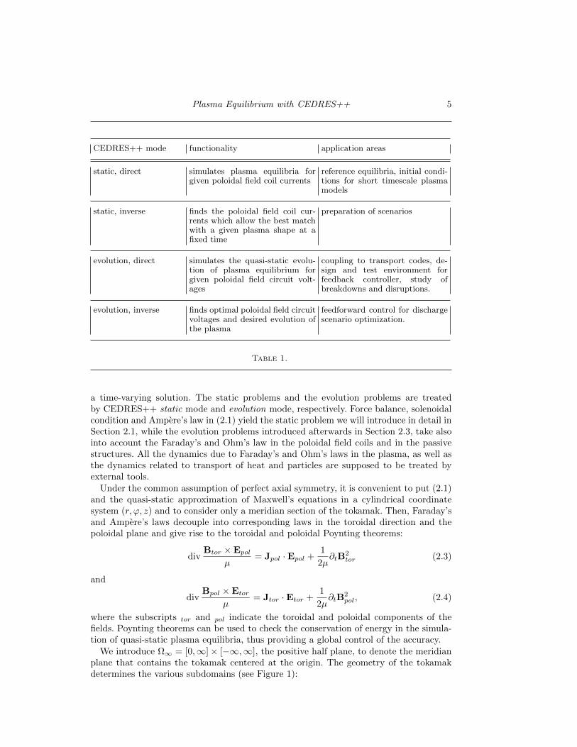
CEDRES++ mode functionality application areas
static, direct simulates plasma equilibria forgiven poloidal field coil currents
reference equilibria, initial condi-tions for short timescale plasmamodels
static, inverse finds the poloidal field coil cur-rents which allow the best matchwith a given plasma shape at afixed time
preparation of scenarios
evolution, direct simulates the quasi-static evolu-tion of plasma equilibrium forgiven poloidal field circuit volt-ages
coupling to transport codes, de-sign and test environment forfeedback controller, study ofbreakdowns and disruptions.
evolution, inverse finds optimal poloidal field circuitvoltages and desired evolution ofthe plasma
feedforward control for dischargescenario optimization.
Table 1.
a time-varying solution. The static problems and the evolution problems are treatedby CEDRES++ static mode and evolution mode, respectively. Force balance, solenoidalcondition and Ampere’s law in (2.1) yield the static problem we will introduce in detail inSection 2.1, while the evolution problems introduced afterwards in Section 2.3, take alsointo account the Faraday’s and Ohm’s law in the poloidal field coils and in the passivestructures. All the dynamics due to Faraday’s and Ohm’s laws in the plasma, as well asthe dynamics related to transport of heat and particles are supposed to be treated byexternal tools.
Under the common assumption of perfect axial symmetry, it is convenient to put (2.1)and the quasi-static approximation of Maxwell’s equations in a cylindrical coordinatesystem (r, ϕ, z) and to consider only a meridian section of the tokamak. Then, Faraday’sand Ampere’s laws decouple into corresponding laws in the toroidal direction and thepoloidal plane and give rise to the toroidal and poloidal Poynting theorems:
divBtor ×Epol
µ= Jpol ·Epol +
1
2µ∂tB
2tor (2.3)
and
divBpol ×Etor
µ= Jtor ·Etor +
1
2µ∂tB
2pol, (2.4)
where the subscripts tor and pol indicate the toroidal and poloidal components of thefields. Poynting theorems can be used to check the conservation of energy in the simula-tion of quasi-static plasma equilibria, thus providing a global control of the accuracy.
We introduce Ω∞ = [0,∞]× [−∞,∞], the positive half plane, to denote the meridianplane that contains the tokamak centered at the origin. The geometry of the tokamakdetermines the various subdomains (see Figure 1):

6 H. Heumann et. al.
r
ΩFe
zΩci,j
Ωpsk
Ωp
ΩL
∂ΩL
0
Figure 1. Left: Geometric description of the tokamak in the poloidal plane. Middle and right:Sketch for characteristic plasma shapes. The plasma boundary touches the limiter (middle) orthe plasma is enclosed by a flux line that goes through an X-point (right).
• the domain ΩFe ⊂ Ω∞ corresponds to those parts that are made of iron; for anair-transformer tokamak ΩFe = ∅;• the domains Ωci,j ⊂ Ω∞, 1 6 i 6 L, 1 6 j 6 Ni, correspond to the
∑Li=1Ni = N
poloidal field coils. The coils are grouped into L poloidal field circuits and the ith circuitcontains Ni coils. The intersection of the jth coil in the ith circuit with the poloidalplane is Ωci,j , and it has ni,j wire turns, total resistance Ri,j and cross section area Si,j ;• the domains Ωpsk ⊂ Ω∞ , k = 1, ..., Nps corresponding to Nps passive structures
with conductivity σk;• the domain ΩL ⊂ Ω∞, bounded by the limiter, corresponds to the domain which is
accessible by the plasma;• the domain Ωp ⊂ ΩL, is the domain covered by the plasma.
The classical primal unknowns for toroidal plasma equilibria described by (2.1) arethe poloidal magnetic flux ψ = ψ(r, z), the pressure p and the diamagnetic function f .The poloidal magnetic flux ψ := rA · eϕ is the scaled toroidal component of the vectorpotential A, i.e. B = curl A and eϕ the unit vector for ϕ. The diamagnetic functionf = rB · eϕ is the scaled toroidal component of the magnetic field. It can be shownthat both the pressure p and the diamagnetic function f are constant on ψ -isolines,i.e. p = p(ψ) and f = f(ψ). We refer to standard text books, e.g. (Freidberg 1987),(Blum 1987), (Wesson 2004), (Goedbloed & Poedts 2004), (Goedbloed et al. 2010) and(Jardin 2010) for the details and state in the following paragraphs only the final equationsdescribing the static and evolution problems solved in CEDRES++.
2.1. Direct Static Problem
Force balance, solenoidal condition and Ampere’s law in (2.1) yield in axisymmetricconfiguration the following set of equations:
−∇ ·(
1
µr∇ψ)
=
rp′(ψ) + 1
µ0rff ′(ψ) in Ωp(ψ) ;
Ii,jSi,j
in Ωci,j ;
0 elsewhere ,
ψ(0, z) = 0 ; lim‖(r,z)‖→+∞
ψ(r, z) = 0 ;
(2.5)
Plasma Equilibrium with CEDRES++ 7
where ∇ is the gradient in the two dimensions (r, z), Ii,j is the total current (in Ampereturns) in the j-th coil of the ith circuit and µ is a functional of ψ
µ =
µFe(|∇ψ|2r−2) in ΩFe
µ0 elsewhere .(2.6)
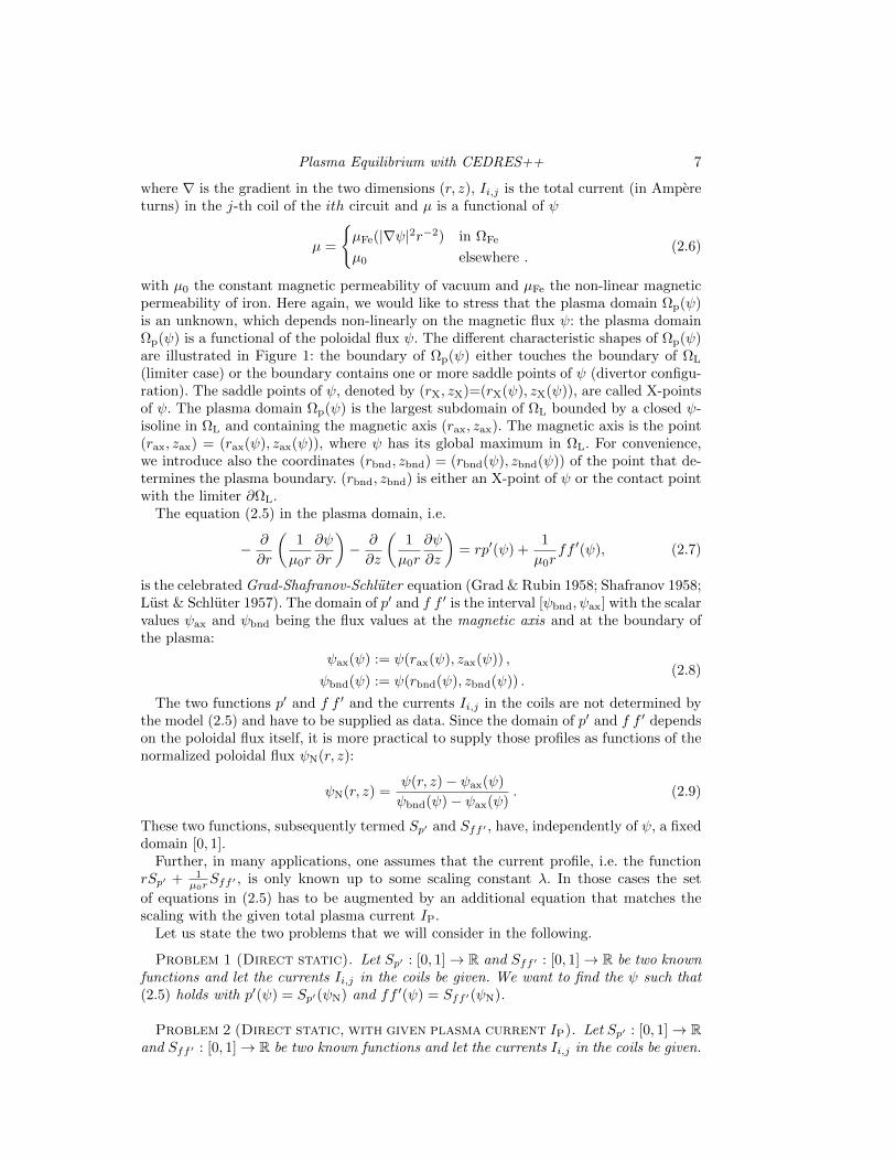
with µ0 the constant magnetic permeability of vacuum and µFe the non-linear magneticpermeability of iron. Here again, we would like to stress that the plasma domain Ωp(ψ)is an unknown, which depends non-linearly on the magnetic flux ψ: the plasma domainΩp(ψ) is a functional of the poloidal flux ψ. The different characteristic shapes of Ωp(ψ)are illustrated in Figure 1: the boundary of Ωp(ψ) either touches the boundary of ΩL
(limiter case) or the boundary contains one or more saddle points of ψ (divertor configu-ration). The saddle points of ψ, denoted by (rX, zX)=(rX(ψ), zX(ψ)), are called X-pointsof ψ. The plasma domain Ωp(ψ) is the largest subdomain of ΩL bounded by a closed ψ-isoline in ΩL and containing the magnetic axis (rax, zax). The magnetic axis is the point(rax, zax) = (rax(ψ), zax(ψ)), where ψ has its global maximum in ΩL. For convenience,we introduce also the coordinates (rbnd, zbnd) = (rbnd(ψ), zbnd(ψ)) of the point that de-termines the plasma boundary. (rbnd, zbnd) is either an X-point of ψ or the contact pointwith the limiter ∂ΩL.
The equation (2.5) in the plasma domain, i.e.
− ∂
∂r
(1
µ0r
∂ψ
∂r
)− ∂
∂z
(1
µ0r
∂ψ
∂z
)= rp′(ψ) +
1
µ0rff ′(ψ), (2.7)
is the celebrated Grad-Shafranov-Schluter equation (Grad & Rubin 1958; Shafranov 1958;Lust & Schluter 1957). The domain of p′ and f f ′ is the interval [ψbnd, ψax] with the scalarvalues ψax and ψbnd being the flux values at the magnetic axis and at the boundary ofthe plasma:
ψax(ψ) := ψ(rax(ψ), zax(ψ)) ,
ψbnd(ψ) := ψ(rbnd(ψ), zbnd(ψ)) .(2.8)
The two functions p′ and f f ′ and the currents Ii,j in the coils are not determined bythe model (2.5) and have to be supplied as data. Since the domain of p′ and f f ′ dependson the poloidal flux itself, it is more practical to supply those profiles as functions of thenormalized poloidal flux ψN(r, z):
ψN(r, z) =ψ(r, z)− ψax(ψ)
ψbnd(ψ)− ψax(ψ). (2.9)
These two functions, subsequently termed Sp′ and Sff ′ , have, independently of ψ, a fixeddomain [0, 1].
Further, in many applications, one assumes that the current profile, i.e. the functionrSp′ + 1
µ0rSff ′ , is only known up to some scaling constant λ. In those cases the set
of equations in (2.5) has to be augmented by an additional equation that matches thescaling with the given total plasma current IP.
Let us state the two problems that we will consider in the following.
Problem 1 (Direct static). Let Sp′ : [0, 1]→ R and Sff ′ : [0, 1]→ R be two knownfunctions and let the currents Ii,j in the coils be given. We want to find the ψ such that(2.5) holds with p′(ψ) = Sp′(ψN) and ff ′(ψ) = Sff ′(ψN).
Problem 2 (Direct static, with given plasma current IP). Let Sp′ : [0, 1]→ Rand Sff ′ : [0, 1]→ R be two known functions and let the currents Ii,j in the coils be given.
8 H. Heumann et. al.
Additionally we assume that the total plasma current IP is given. We want to find ψ andλ such that (2.5) holds with p′(ψ) = λSp′(ψN) and ff ′(ψ) = λSff ′(ψN) together with
IP = λ
∫Ωp(ψ)
(rSp′(ψN(r, z)) +
1
µ0rSff ′(ψN(r, z))
)drdz. (2.10)
The functions Sp′ and Sff ′ are usually given as piecewise polynomial functions. An-other frequent a priori model is
Sp′(ψN) =β
r0(1− ψαN)γ , Sff ′(ψN) = (1− β)µ0r0(1− ψαN)γ , (2.11)
with r0 the major radius of the vacuum chamber and α, β, γ ∈ R given parameters. Werefer to (Luxon & Brown 1982) for a physical interpretation of these parameters. Theparameter β is related to the poloidal beta, whereas α and γ describe the peakage of thecurrent profile.
2.2. Inverse Static Problem
The direct problem in the previous section computes a free-boundary equilibrium forgiven coil currents. In many applications, in particular in the area of tokamak operation,the inverse problem is equally relevant: What are the currents that give a certain desiredshape to the plasma? A popular approach to answer such a question is its formulationas an optimal control problem. The currents Ii in the poloidal field coils are the controlvariables and the magnetic flux map ψ describing the equilibrium is the controlled vari-able. Then we introduce a cost function for the magnetic flux ψ and the coil currents Iipenalizing the deviation from a desired plasma shape and position, and we minimize thiscost function under the constraint that the magnetic flux ψ and the currents in the coilssolve the equilibrium problem (2.5). A regularization term ensures well-posedness of theinverse problem. Here again, the current profile in the plasma is supposed to be knowndata.
In CEDRES++ we prescribe a plasma state by a desired plasma boundary Γdesi. LetΓdesi ⊂ ΩL denote a closed line, contained in the domain ΩL that is either smooth andtouches the limiter at one point or has at least one corner. The former case prescribesa desired plasma boundary that touches the limiter. The latter case aims at a plasmawith X-point lying entirely in the interior of ΩL. Further let (rdesi, zdesi) ∈ Γdesi and(r1, z1), . . . (rNdesi
, zNdesi) ∈ Γdesi be Ndesi + 1 points on that line. We define a quadratic
cost functional K(ψ) that evaluates to zero if Γdesi is a ψ-isoline, i.e. if ψ is constant onΓdesi:
K(ψ) :=1
2
Ndesi∑i=1
(ψ(ri, zi)− ψ(rdesi, zdesi)
)2. (2.12)
Another quadratic cost functional, that will serve as regularization, is
R(I1,1, . . . , IL,NL) :=
L∑i=1
Ni∑j=1
wi,j2I2i,j . (2.13)
The coefficients wi,j > 0 are called regularization weights.Let us state the two inverse problems that we will consider in the following.
Problem 3 (Inverse static). Let Sp′ : [0, 1] → R and Sff ′ : [0, 1] → R be two

Plasma Equilibrium with CEDRES++ 9
known functions. We solve the following minimization problem:
minψ,I1,1,...IL,NL
K(ψ) +R(I1,1, . . . IL,NL) subject to (2.5) (2.14)
with p′(ψ) = Sp′(ψN) and ff ′(ψ) = Sff ′(ψN).
Problem 4 (Inverse static, with given plasma current IP). Let Sp′ : [0, 1]→R and Sff ′ : [0, 1] → R be two known functions and assume additionally that the totalplasma current IP is given. We solve the following minimization problem:
minλ,ψ,I1,1,...IL,NL
K(ψ) +R(I1,1, . . . IL,NL) subject to (2.5) and (2.10) (2.15)
with p′(ψ) = λSp′(ψN) and ff ′(ψ) = λSff ′(ψN).
Clearly, it is also possible to define other cost functions forcing the plasma to haveother characteristics. CEDRES++ can be easily extended in this direction. Furthermoreit is possible to add both equality and inequality constraints. We are planning to includefor example upper and lower bounds on the currents and the forces in the coils.
Another class of inverse problems related to static equilibrium, appears in real timetokamak control. There, it is important to reconstruct both the plasma boundary as wellas the current profile functions p′ and ff ′ in the plasma from external measurements.Frequent and fast prediction of the current state of the plasma in the tokamak machine areessential information for feedback control system. Hence, the computational challengesin solving these inverse problems are much different, and lead to the development of aseparate class of equilibrium codes (Hofmann & Tonetti 1988; Lao et al. 1990; Mc Carthyet al. 1999; Blum et al. 2012).
2.3. Direct Evolution Problem
In contrast to the static problems, the evolution problems in CEDRES++ take alsointo account the Faraday’s and Ohm’s laws in the poloidal field coils and in the passivestructures. The dynamics due to Faraday’s and Ohm’s law in the plasma, as well asthe dynamics related to transport of heat and particles are supposed to be treated byexternal tools. Alternatively, one can prescribe the profiles Sp′ and Sff ′ as functionsof time. The Poynting theorems (2.4) and (2.3) could provide a global mean to checkwhether the coupling between CEDRES++ and such external tools is accurate. However,due to discretization, one needs to resort to integrated versions of the Poynting theoremsfor the accuracy check. Later, in section 3.6, we will present detailed formulas of suchintegrated Poynting theorems.
The N poloidal field coils are gathered into L poloidal field circuits which contain intotal M supplies. Each of the L poloidal field circuits contains a subset of the N coils anda subset of the M supplies. We denote by ~Ii the vector of size Mi + Ni which containsthe currents at the Mi supplies and in the Ni coils of the circuit with index i, 1 6 i 6 L.The circuit equations in the ith circuit can be written in the form:
~Ii = Si~Vi + Ri~Ψi(∂tψ) , (2.16)
where the matrices Si ∈ R(Mi+Ni)×Mi and Ri ∈ R(Mi+Ni)×Ni depend on the wire turnsni,·, the total resistances Ri,· and the cross sections Si,· of the poloidal field coils in thecircuit i and on the topology of the circuit. Details on the computation of matrices Si andRi are given in Appendix (A). The vectors ~Vi ∈ RMi contain the voltages applied to the
supplies, and the vectors ~Ψi(ψ) ∈ RNi are ~Ψi(ψ) = (∫
Ωci,1ψdrdz, . . . ,
∫Ωci,Ni
ψdrdz)T .
10 H. Heumann et. al.
In the case of a simple circuit composed of one supply connected to the coil Ωci,1 theequation (2.16) writes
Ii,1 =ni,1Vi,1(t)
Ri,1− 2π
n2i,1
Ri,1Si,1
∫Ωci,1
∂ψ
∂tdrdz .
The free-boundary equilibrium problem on the time interval [0, T ] for the time dependentpoloidal flux ψ = ψ(t) = ψ(r, z, t) is:
−∇ ·(
1
µr∇ψ)
=
rp′(ψ, t) + 1
µ0rff ′(ψ, t) in Ωp(ψ) ;
S−1i,j
(Si~Vi + Ri
~Ψi(∂tψ))j
in Ωci,j , 1 6 i 6 L, 1 6 j 6 Ni;
−σkr∂ψ∂t in Ωpsk ;
0 elsewhere ,
ψ(0, z, t) = 0 ; lim‖(r,z)‖→+∞
ψ(r, z, t) = 0 ;
ψ(r, z, 0) = ψ0(r, z) ,(2.17)
The equation in the passive structures Ωpsk is deduced from Ohm’s law and Faraday’slaw, σk being the equivalent axi-symmetric conductivity.
Problem 5 (Evolution, direct). Let Sp′ : [0, 1] × [0, T ] → R and Sff ′ : [0, 1] ×[0, T ]→ R be two known functions. Let the evolution of the voltages ~V1(t), . . . , ~VL(t) in thepoloidal field circuits and the initial data ψ0 be given. We want to find the evolution of ψ(t)such that (2.17) holds with p′(ψ(t), t) = λSp′(ψN(t), t) and ff ′(ψ(t), t) = λSff ′(ψN(t), t).
Problem 6 (evolution, with given plasma current IP(t), direct). Let Sp′ :[0, 1]×[0, T ]→ R and Sff ′ : [0, 1]×[0, T ]→ R be two known functions. Let the evolution of
the voltages ~V1(t), . . . , ~VL(t) in the poloidal field circuits and the initial data ψ0 be given.Additionally we assume that the evolution of the total plasma current IP(t) is given.We want to find the evolution of ψ(t) and λ(t) such that (2.17) holds with p′(ψ(t), t) =λSp′(ψN(t), t) and ff ′(ψ(t), t) = λSff ′(ψN(t), t) together with
IP(t) = λ(t)
∫Ωp(ψ(t))
(rSp′(ψN(r, z, t), t) +
1
µ0rSff ′(ψN(r, z, t), t)
)drdz. (2.18)
To model a consistent quasi-static evolution of plasma equilibrium the equations in(2.17) have to be augmented by the diffusion of density, temperature and magnetic flux.In that case, both functions Sp′ and Sff ′ in the Problems 5 and 6 appear as unknownsof the full system of equations.
2.4. Inverse Evolution Problem
The inverse evolution problem is the problem of determining external voltages such thatthe evolution of the plasma has certain prescribed properties. We will state this problemagain as an optimal control problem.
Let Γdesi(t) ⊂ ΩL denote the evolution of a closed line, contained in the domain ΩL
that is either smooth and touches the limiter at one point or has at least one corner.The former case prescribes a desired plasma boundary that touches the limiter. Thelatter case aims at a plasma with X-point that is entirely in the interior of ΩL. Furtherlet (rdesi(t), zdesi(t)) ∈ Γdesi(t) and (r1(t), z1(t)), . . . , (rNdesi
(t), zNdesi(t)) ∈ Γdesi(t) be

Plasma Equilibrium with CEDRES++ 11
Ndesi + 1 points on that line. We define a quadratic functional K(ψ) that evaluates tozero if Γdesi(t) is an ψ(t)-isoline, i.e. if ψ(t) is constant on Γdesi(t):
K(ψ(t)) :=1
2
∫ T
0
(Ndesi∑i=1
(ψ(ri(t), zi(t), t)− ψ(rdesi(t), zdesi(t), t)
)2)dt. (2.19)
Another functional, that will serve as regularization, is
R(~V1(t), . . . , ~VL(t)) :=
L∑i=1
wi2
∫ T
0
~Vi(t) · ~Vi(t)dt. (2.20)
It penalizes the strength of the voltages ~Vi and represents the energetic cost in the coilsystem. The coefficients wi > 0 are called regularization weights.
Problem 7 (Evolution, inverse). Let Sp′ : [0, 1]×[0, T ]→ R and Sff ′ : [0, 1]×R→R be two known functions. We solve the following minimization problem:
minψ(t),~V1(t),...~VL(t)
K(ψ(t)) +R(~V1(t), . . . ~VL(t)) subject to (2.17) (2.21)
with p′(ψ(t), t) = Sp′(ψN(t), t) and ff ′(ψ(t)) = Sff ′(ψN(t), t).
Problem 8 (Evolution, with given plasma current IP(t), inverse). Let Sp′ :[0, 1] × [0, T ] → R and Sff ′ : [0, 1] × R → R be two known functions. Additionallywe assume that the evolution of the total plasma current IP(t) is given. We solve thefollowing minimization problem:
minλ(t),ψ(t),~V1(t),...~VL(t)
K(ψ(t)) +R(~V1(t), . . . ~VL(t)) subject to (2.17) and (2.18) (2.22)
with p′(ψ(t), t) = λ(t)Sp′(ψN(t), t) and ff ′(ψ(t)) = λ(t)Sff ′(ψN(t), t).
3. Computational Methods and Applications
The main challenges for solving the Problems 1-8 numerically are their formulationon an infinite domain, the non-linear right-hand side, the non-linear permeability in ironand the non-linearity due to the free plasma boundary. In the following we will use finiteelement methods (Ciarlet 1978) to discretize the problems 1-8, and we will see that thisapproach is flexible enough to tackle all those challenges at once. First, finite elementmethods are favored approximation methods due to their flexibility on domains withcomplex geometry. Second, they allow for a straight forward implementation of New-ton methods to handle the strong non-linearities related to the free boundary setting.The convergence speed of such Newton methods is superior to the convergence speed offixed-point approaches that are otherwise applied for such kind of problems. As a varia-tional formulation is the starting point for any finite element method the section startswith the variational formulations of Problems 1, 2, 5 and 6. The subsequent paragraphon the spatial discretization, a standard finite element method with linear Lagrangianbasis functions on triangles, focuses mainly on the special treatment of the free plasmaboundary. It gives the important formulas, required to derive the new Newton methodafterwards. Having these Newton methods at hand, it is straightforward to tackle theinverse problems. The overview on the computational methods finishes with two para-graphs describing the interfaces of CEDRES++ for the coupling with transport codesand presenting volume integrated Poynting theorems.

12 H. Heumann et. al.
3.1. Variational Formulation on the Truncated Domain
We chose a semi-circle Γ of radius ρΓ surrounding the iron domain ΩFe, the coil domainsΩci,j and the passive structures domain Ωpsk . The truncated domain, we use for ourcomputations, is the domain Ω ⊂ Ω∞ having the boundary ∂Ω = Γ ∪ Γr=0, whereΓr=0 := (r, z) , r = 0. The variational formulations of Problems 1, 2, 5 and 6 use thefollowing Sobolev space:
V :=
ψ : Ω→ R,
∫Ω
ψ2r drdz <∞,∫
Ω
(∇ψ)2r−1 drdz <∞, ψ|Γr=0= 0
∩C0(Ω) (3.1)
and are obtained by multiplying equations in 1, 2, 5 and 6 by testfunctions ξ ∈ V andintegrating by parts over Ω. They are called the variational formulations since they arethe Euler equations of the mininization of the energy. Then we define• two mappings A : V × V → R and Jp : V × V → R that are linear in the last
argument:
A(ψ, ξ) :=
∫Ω
1
µ(ψ)r∇ψ · ∇ξ drdz
Jp(ψ, ξ) :=
∫Ωp(ψ)
(rp′(ψ) +
1
µ0rff ′(ψ)
)ξ drdz (3.2)
• two bilinear forms jps, jc : V × V → R
jps(ψ, ξ) := −Nps∑i=1
∫Ωpsk
σkrψξ drdz
jc(ψ, ξ) :=
L∑i=1
Ni∑j=1
S−1i,j
(Ri~Ψi(ψ)
)j
∫Ωci,j
ξ drdz
(3.3)
• N bilinear mappings `i,j : R× V → R:
`i,j(I, ξ) := S−1i,j I
∫Ωci,j
ξ drdz (3.4)
• a bilinear form c : V × V → R, accounting for the boundary conditions at infinity(Albanese et al. 1986):
c(ψ, ξ) :=1
µ0
∫Γ
ψ(P1)N(P1)ξ(P1)dS1
+1
2µ0
∫Γ
∫Γ
(ψ(P1)− ψ(P2))M(P1,P2)(ξ(P1)− ξ(P2))dS1dS2.
(3.5)
with
M(P1,P2) =kP1,P2
2π(r1r2)32
(2− k2
P1,P2
2− 2k2P1,P2
E(kP1,P2)−K(kP1,P2
)
)
N(P1) =1
r1
(1
δ++
1
δ−− 1
ρΓ
)and δ± =
√r21 + (ρΓ ± z1)2 ,
where Pi = (ri, zi) and K and E the complete elliptic integrals of first and second kind,respectively and
kPj ,Pk =
√4rjrk
(rj + rk)2 + (zj − zk)2.
Plasma Equilibrium with CEDRES++ 13
We refer to (Grandgirard 1999, Chapter 2.4) for the details of the derivation. The bilinearform c(·, ·) follows basically from the so called uncoupling procedure in (Gatica & Hsiao1995) for the usual coupling of boundary integral and finite element methods. In our case,it can be shown that for all P1, P2 the integral term (ψ(P1)−ψ(P2))M(P1,P2)(ξ(P1)−ξ(P2)) remains bounded. The Green’s function that is used in the derivation of theboundary integral method for our problem was used earlier in finite difference methodsfor the Grad-Shafranov-Schluter equations (Lackner 1976).We derive the following variational formulations of the direct Problems 1 and 2.
Variational Formulation 9 (Static). Let Sp′ : [0, 1]→ R and Sff ′ : [0, 1]→ R betwo known functions and let the currents Ii,j in the coils be given. We set p′(ψ) = Sp′(ψN)and ff ′(ψ) = Sff ′(ψN) in (3.2). We want to find ψ ∈ V such that
A(ψ, ξ)− Jp(ψ, ξ) + c(ψ, ξ) =
L∑i=1
Ni∑j=1
`i,j(Ii,j , ξ) (3.6)
holds for all ξ ∈ V .
Variational Formulation 10 (Static, with given plasma current IP). LetSp′ : [0, 1]→ R and Sff ′ : [0, 1]→ R be two known functions and let the currents Ii,j inthe coils be given. We set p′(ψ) = Sp′(ψN) and ff ′(ψ) = Sff ′(ψN) in (3.2). Additionallywe assume that the total plasma current IP is given. We want to find ψ ∈ V and λ ∈ Rsuch that
A(ψ, ξ)− λ Jp(ψ, ξ) + c(ψ, ξ) =
L∑i=1
Ni∑j=1
`i,j(Ii,j , ξ),
Ip − λ Jp(ψ, 1) = 0,
(3.7)
holds for all ξ ∈ V .
The variational formulation of the evolution problems 5 and 6 is based on an implicitEuler timestepping scheme 0 := t0 < t0 + ∆t1 = t1 < . . . tn−1 + ∆tn = tn = T . Otherchoices are possible. Since we will anyway employ only low order spatial discretization,the implicit Euler is the obvious choice.
Variational Formulation 11 (Evolution). Let Sp′ : [0, 1] × [0, T ] → R andSff ′ : [0, 1] × [0, T ] → R be two known functions. Let the evolution of the voltages~V1(t), . . . , ~VL(t) in the poloidal field circuits and the initial data ψ0 be given. We setp′(ψ) = Sp′(ψN(t), t) and ff ′(ψ) = Sff ′(ψN(t), t) in (3.2). We want to find ψk ∈ Vapproximating ψ(tk) such that
∆tkA(ψk, ξ)−∆tkJkp(ψk, ξ)− jps(ψk, ξ)− jc(ψk, ξ) + ∆tkc(ψ
k, ξ)
= ∆tk
L∑i=1
Ni∑j=1
`i,j((Si~Vi(tk))j , ξ)− jps(ψk−1, ξ)− jc(ψk−1, ξ) ,
ψ0 = ψ0 ,
(3.8)
holds for all ξ ∈ V with Jkp(·, ·) = Jp(·, ·)|t=tk .
Variational Formulation 12 (Evolution, with given plasma current IP(t)).Let Sp′ : [0, 1] × [0, T ] → R and Sff ′ : [0, 1] × [0, T ] → R be two known functions. Let
the evolution of the voltages ~V1(t), . . . , ~VL(t) in the poloidal field circuits and the initial
14 H. Heumann et. al.
data ψ0 be given. We set p′(ψ) = Sp′(ψN(t), t) and ff ′(ψ) = Sff ′(ψN(t), t) in (3.2).Additionally we assume that the evolution of the total plasma current IP(t) is given. Wewant to find ψk ∈ V and λk ∈ R approximating ψ(tk) and λ(tk) such that
∆tkA(ψk, ξ)−∆tkλk Jkp(ψk, ξ)− jps(ψk, ξ)− jc(ψk, ξ) + ∆tkc(ψ
k, ξ)
= ∆tk
L∑i=1
Ni∑j=1
`i,j((Si~Vi(tk))j , ξ)− jps(ψk−1, ξ)− jc(ψk−1, ξ),
Ip(tk)− λk Jkp(ψk, 1) = 0, ψ0 = ψ0 .
(3.9)
holds for all ξ ∈ V with Jkp(·, ·) = Jp(·, ·)|t=tk .
3.2. A Galerkin Discretization
We use a standard linear Lagrangian finite element to discretize the non-linear operatorsin the previous section. Finite element methods are particularly well suited to treatcomplex geometries, such as the one of the tokamak (plasma, passive structures, poloidalfield coils.) We refer to section 5 for a general discussion on the choice of the order of thefinite element method. For this we introduce a triangulation Ωh of the domain Ω thatresolves the subdomains ΩL,ΩFe,Ωci,j ,Ωpsk . The finite element approximation ψh of ψin the finite element space Vh is an expansion in basis functions λi:
ψh(r, z) =∑i
ψiλi(r, z) with ψi ∈ R. (3.10)
Each Lagrangian basis function λi(r, z) is piecewise linear and vanishes at all verticesexcept one. The domain of the plasma Ωp(ψh) of a finite element function ψh is boundedby a continuous, polygonal, closed line. The critical points (rbnd(ψh), zbnd(ψh)) and(rax(ψh), zax(ψh)) are the coordinates of certain vertices of the mesh. The saddle pointof a piecewise linear function ψh is some vertex (r0, z0) with the following property: if(r1, z1), (r2, z2) . . . (rn, zn), denote the counterclockwise ordered neighboring vertices thesequence of discrete gradients ψ0 − ψ1, ψ0 − ψ2 . . . ψ0 − ψn changes at least four timesthe sign.
It remains to specify the quadrature rule that is used to approximate integrals overtriangles T and integrals over intersection T∩Ωp(ψh) of triangles with the plasma domain∫
T
f(r, ψh)λidrdz and
∫T∩Ωp(ψh)
g(r, ψh)λidrdz . (3.11)
The second type of integrals appears in JP due to the fact that the mesh does not resolvethe boundary of the plasma domain Ωp. In any case we will use the centers of gravity
bT := (rT , zT ) and bT (ψh) := (rT (ψh), zT (ψh)) := (rT∩Ωp(ψh), zT∩Ωp(ψh)) (3.12)
of the integration domains T or T ∩ Ωp(ψh) as quadrature points. The correspondingquadrature weights are the size of the corresponding domain |T | and |T ∩ Ωp(ψh)|. Thebarycenter for the second type of integrals depends itself on ψh. Our choice of quadraturerule introduces a consistency error of order O(h2), where h is the diameter of the triangle,i.e. the quadrature is exact for linear integrands.
For a triangle T with vertex coordinates ai,aj ,ak ∈ R2 the center of gravity corre-sponds to the barycenter:
(rT , zT ) =1
3(ai + aj + ak). (3.13)
Plasma Equilibrium with CEDRES++ 15
ai
ak aj
∂Ωp
mkmj
ajak
ai
∂Ωp
mk
mj
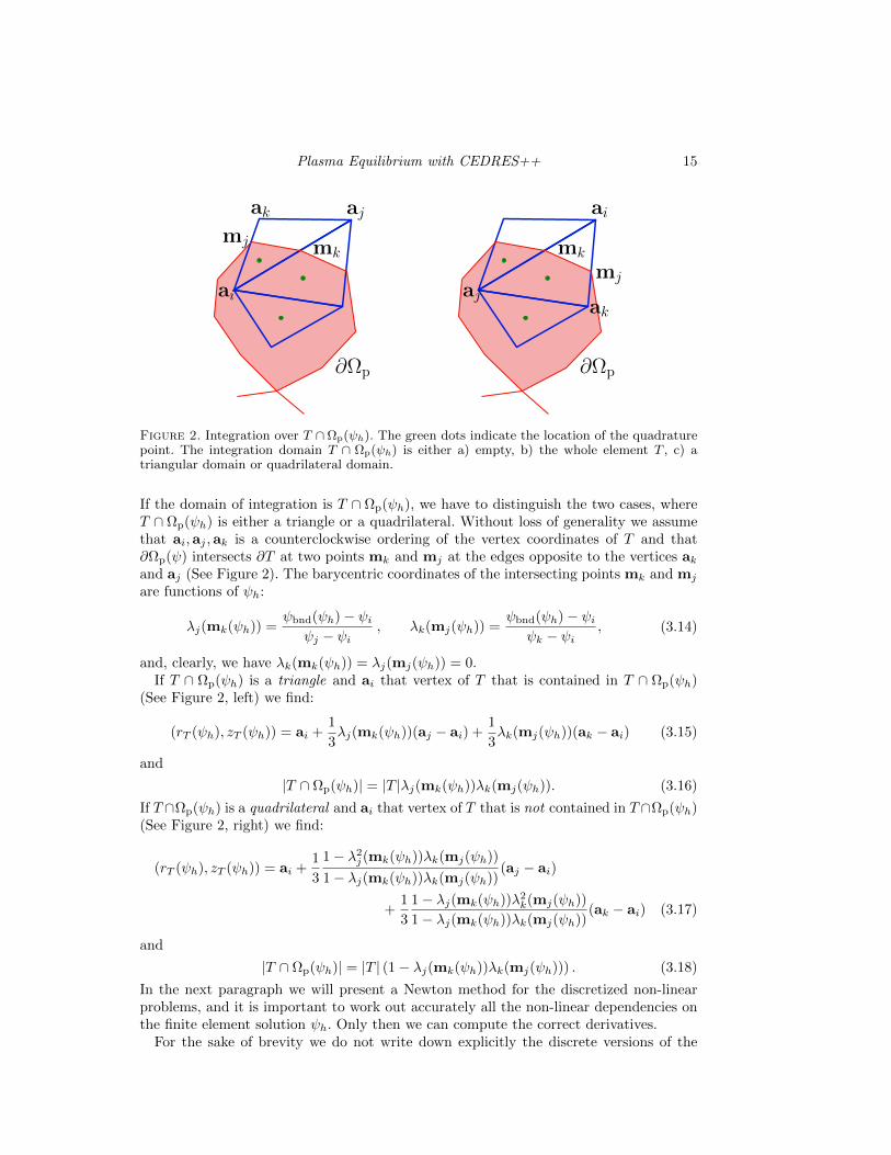
Figure 2. Integration over T ∩Ωp(ψh). The green dots indicate the location of the quadraturepoint. The integration domain T ∩ Ωp(ψh) is either a) empty, b) the whole element T , c) atriangular domain or quadrilateral domain.
If the domain of integration is T ∩ Ωp(ψh), we have to distinguish the two cases, whereT ∩ Ωp(ψh) is either a triangle or a quadrilateral. Without loss of generality we assumethat ai,aj ,ak is a counterclockwise ordering of the vertex coordinates of T and that∂Ωp(ψ) intersects ∂T at two points mk and mj at the edges opposite to the vertices akand aj (See Figure 2). The barycentric coordinates of the intersecting points mk and mj
are functions of ψh:
λj(mk(ψh)) =ψbnd(ψh)− ψi
ψj − ψi, λk(mj(ψh)) =
ψbnd(ψh)− ψiψk − ψi
, (3.14)
and, clearly, we have λk(mk(ψh)) = λj(mj(ψh)) = 0.If T ∩ Ωp(ψh) is a triangle and ai that vertex of T that is contained in T ∩ Ωp(ψh)
(See Figure 2, left) we find:
(rT (ψh), zT (ψh)) = ai +1
3λj(mk(ψh))(aj − ai) +
1
3λk(mj(ψh))(ak − ai) (3.15)
and
|T ∩ Ωp(ψh)| = |T |λj(mk(ψh))λk(mj(ψh)). (3.16)
If T ∩Ωp(ψh) is a quadrilateral and ai that vertex of T that is not contained in T ∩Ωp(ψh)(See Figure 2, right) we find:
(rT (ψh), zT (ψh)) = ai +1
3
1− λ2j (mk(ψh))λk(mj(ψh))
1− λj(mk(ψh))λk(mj(ψh))(aj − ai)
+1
3
1− λj(mk(ψh))λ2k(mj(ψh))
1− λj(mk(ψh))λk(mj(ψh))(ak − ai) (3.17)
and
|T ∩ Ωp(ψh)| = |T | (1− λj(mk(ψh))λk(mj(ψh))) . (3.18)
In the next paragraph we will present a Newton method for the discretized non-linearproblems, and it is important to work out accurately all the non-linear dependencies onthe finite element solution ψh. Only then we can compute the correct derivatives.
For the sake of brevity we do not write down explicitly the discrete versions of the
16 H. Heumann et. al.
operators from the previous paragraph, but introduce the subcript h to denote the dis-cretized non-linear operators. Ah for example is the discretized version of A. We get fullydiscrete non-linear formulations.
Galerkin Formulation 13 (Static). Let Sp′ : [0, 1] → R and Sff ′ : [0, 1] → R betwo known functions and let the currents Ii in the coils be given. We set p′(ψ) = Sp′(ψN)and ff ′(ψ) = Sff ′(ψN) in (3.2). We want to find ψh ∈ Vh such that
Ah(ψh, ξh)− Jp,h(ψh, ξh) + ch(ψh, ξh) =
L∑i=1
Ni∑j=1
`i,j,h(Ii,j , ξh) (3.19)
holds for all ξh ∈ Vh.
Galerkin Formulation 14 (Static, with fixed plasma current IP). Let Sp′ :[0, 1] → R and Sff ′ : [0, 1] → R be two known functions and let the currents Ii in thecoils be given. We set p′(ψ) = Sp′(ψN) and ff ′(ψ) = Sff ′(ψN) in (3.2). Additionally weassume that the total plasma current IP is given. We want to find ψh ∈ Vh and λ ∈ Rsuch that
Ah(ψh, ξh)− λ Jp,h(ψh, ξh) + ch(ψh, ξh) =
L∑i=1
Ni∑j=1
`i,j,h(Ii,j , ξh),
Ip − λ Jp,h(ψh, 1) = 0,
(3.20)
holds for all ξh ∈ Vh.
Galerkin Formulation 15 (Evolution). Let Sp′ : [0, 1] × [0, T ] → R and Sff ′ :
[0, 1]× [0, T ] → R be two known functions. Let the evolution of the voltages ~Vi(t) in thepoloidal field circuits and the initial data ψ0 be given. We set p′(ψ) = Sp′(ψN(t), t) andff ′(ψ) = Sff ′(ψN(t), t) in (3.2). We want to find ψkh ∈ Vh approximating ψ(tk) such that
∆tkAh(ψkh, ξh)−∆tkJkp,h(ψkh, ξh)− jps
h (ψkh, ξh)− jch(ψkh, ξh) + ∆tkc(ψkh, ξh)
= ∆tk
L∑i=1
Ni∑j=1
`i,j,h((Si~Vi(tk))j , ξh)− jpsh (ψk−1
h , ξh)− jch(ψk−1h , ξh),
ψ0h = ψ0
(3.21)
holds for all ξh ∈ Vh with Jkp,h(·, ·) = Jp,h(·, ·)|t=tk .
Galerkin Formulation 16 (Evolution, with given plasma current IP(t)).Let Sp′ : [0, 1] × [0, T ] → R and Sff ′ : [0, 1] × [0, T ] → R be two known functions. Let
the evolution of the voltages ~Vi(t) in the poloidal field circuits and the initial data ψ0 begiven. We set p′(ψ) = Sp′(ψN(t), t) and ff ′(ψ) = Sff ′(ψN(t), t) in (3.2). Additionallywe assume that the evolution of the total plasma current IP(t) is given. We want to findψkh ∈ Vh and λk ∈ R approximating ψ(tk) and λ(tk) such that
∆tkAh(ψkh, ξh)−∆tkJkp,h(ψkh, ξh)− jps
h (ψkh, ξh)− jc,h(ψkh, ξh) + ∆tkc(ψkh, ξh)
= ∆tk
L∑i=1
Ni∑j=1
`ci,j,h((Si~Vi(tk))j , ξh)− jpsh (ψk−1
h , ξh)− jc,h(ψk−1h , ξh),
Ip(tk)− λk Jkp,h(ψkh, 1) = 0, ψ0h = ψ0 ,
(3.22)
holds for all ξ ∈ Vh with Jkp,h(·, ·) = Jp,h(·, ·)|t=tk .
Plasma Equilibrium with CEDRES++ 17
The Galerkin formulations assume that the function µFe is known. In practical ap-plications µFe needs to be estimated from experimental data. We refer to (Glowinski &Marrocco 1974) and, more recently (Pechstein & Juttler 2006), for details.
3.3. Newton’s Method and the Free Plasma Boundary
Newton’s methods for solving a non-linear problem F (x) = 0 for x is the followingiterative scheme:
F ′(xi)(xi+1 − xi) = −F (xi) ⇔ F ′(xi)xi+1 = F ′(xi)xi − F (xi). (3.23)
If F is sufficiently smooth, standard theory for Newton methods asserts that this iterationconverges quadratically fast to the solution x. In our case the magnetic flux ψ or its finiteelement approximation ψh plays the role of the unknown x. If we want to apply thismethod to either our continuous non-linear variational formulations 9, 10, 11 and 12 orthe discretized versions, namely the Galerkin Formulations 13, 14, 15 and 16, we need tocompute derivatives of the non-linear operators.
For the continuous formulations we need to calculate all the directional derivativesDψA(ψ, ξ)(ψ), DψJp(ψ, ξ)(ψ), Dψj
ps(ψ, ξ)(ψ), Dψjc(ψ, ξ)(ψ) and Dψc(ψ, ξ)(ψ). This cal-
culation is simple for the bilinear mappings jc, jps, e.g.,
Dψjps(ψ, ξ)(ψ) = jps(ψ, ξ), Dψj
c(ψ, ξ)(ψ) = jc(ψ, ξ), (3.24)
and the non-linear mapping A (see (2.6)):
DψA(ψ, ξ)(ψ) =
∫Ω
1
µ(ψ)r∇ψ·∇ξ drdz−2
∫ΩFe
µ′Fe(| gradψ|2r−2)
µ2Fe(| gradψ|2r−2)r3
∇ψ·∇ψ∇ψ·∇ξ drdz.
The remaining derivative of Jp was given in (Blum 1987, Lemma I.4):
DψJp(ψ, ξ)(ψ) =
∫Ωp(ψ)
∂jp(r, ψN(ψ))
∂ψN
∂ψN(ψ)
∂ψψ ξ drdz,
−∫
Γp(ψ)
jp(r, 1)|∇ψ|−1(ψ − ψ(rbnd(ψ), zbnd(ψ)))ξ dΓ
+
∫Ωp(ψ)
∂jp(r, ψN(ψ))
∂ψN
∂ψN(ψ)
∂ψaxψ(rax(ψ), zax(ψ))ξ drdz,
+
∫Ωp(ψ)
∂jp(r, ψN(ψ))
∂ψN
∂ψN(ψ)
∂ψbndψ(rbnd(ψ), zbnd(ψ))ξ drdz ,
(3.25)
where Γp is the plasma boundary ∂Ωp and
jp(r, ψN(ψ)) = rSp′(ψN(ψ)) +1
µ0rSff ′(ψN(ψ)) . (3.26)
The derivation involves shape calculus (Murat & Simon 1976; Delfour & Zolesio 2011)and the non-trival derivatives:
Dψψax(ψ)(ψ) = ψ(rax(ψ), zax(ψ)) and Dψψbnd(ψ)(ψ) = ψ(rbnd(ψ), zbnd(ψ)) .
The formula of the derivative relies on certain smoothness assumptions on ψ. Up toour knowledge, there is no theoretical evidence that this formula holds also for plasmaequilibria with boundaries that contain X-points. In particular the second term on theright hand side seems to blow up if ψ reaches a critical point.
Also in (Blum 1987), it is shown that the derivative of Jp(ψ, ξ) in the direction ψ
18 H. Heumann et. al.
vanishes: DψJp(ψ, ξ)(ψ) = 0. Then the Newton scheme for solving Problem 10 is thefollowing iteration: Let (ψn, λn) be the solution at the n-th iteration. For given (ψn, λn)we introduce the linear form:
Fn(ξ) := −A(ψn, ξ) +DψA(ψn, ξ)(ψn) +
L∑i=1
Ni∑j=1
`ci,j(Ii,j , ξ)
= −2
∫ΩFe
µ′Fe(|∇ψ|2r−2)
µ2Fe(|∇ψ|2r−2)r3
|∇ψn|2∇ψn · ∇ξ drdz +
L∑i=1
Ni∑j=1
`ci,j(Ii,j , ξ).
(3.27)
and the Newton update (ψn+1, λn+1) is the solution of the infinite dimensional linearsystem
DψA(ψn, ξ)(ψn+1)− λnDψJp(ψn, ξ)(ψn+1) + c(ψn+1, ξ)− Jp(ψn, ξ)λn+1 = Fn(ξ), ∀ξ ∈ VλnDψJp(ψn, 1)(ψn+1) + Jp(ψn, 1)λn+1 = Ip
After each iteration we need to recompute ψax(ψn) = ψn(rax(ψn), zax(ψn)), ψbnd(ψn) =ψ(rbnd(ψn), zbnd(ψn)) and Ωp(ψn). For the computation of the initial flux function ψ0
we choose a constant permeability in iron and replace the non-linear form Jp(ψ, ξ) withsome linear form
∫Ωpjinitξ drdz, where Ωp is a given ellipse and jinit a given constant
current density. Hence ψ0 is the solution to a linear problem and determines the plasmaaxis and the plasma boundary in the first Newton iteration.
The Newton iterations for the Problems 9, 11 and 12 follow likewise. The equilib-rium codes SCED (Blum et al. 1981) and Proteus (Albanese et al. 1987) are based ondiscretizations of such Newton iterations. The flux functions ψn and ψn+1 are approx-imated by finite weighted sums of finite element basis functions and the test functionsξ cycle over all test functions. In each Newton iteration, one has to invert an algebraicsystem whose size is equal to the number of finite element basis functions. But since it isnot clear, whether the formula for the derivative of Jp(ψ, ξ)(ψ) remains valid for plasmaboundaries with X-points, these approaches are not very trustworthy.
In CEDRES++ we prefer to use Newton methods for the Galerkin Formulations 13,14, 15 and 16. Such Newton methods need the directional derivatives DψhAh(ψh, ξh)(ψh),
DψhJp,h(ψh, ξh)(ψh),Dψh jpsh (ψh, ξh)(ψh),Dψh j
ch(ψh, ξh)(ψh) andDψhch(ψh, ξh)(ψh). Here
again, this is a straightforward and simple calculation for all mappings except one: themapping JP,h that is related to the non-linear current profile in the plasma domain. Themapping JP,h is given by
JP,h(ψh, λm) =∑
TJTP,h(ψh, λm) :=
∑T|T ∩ Ωp(ψh)| jp(bT (ψh))λm(bT (ψh)),
where jp(bT (ψh)) = jp(rT (ψh), ψN(ψh(bT (ψh)), ψax(ψh), ψbnd(ψh))). The directionalderivative of JP,h(ψh, λm) in direction λn is the partial derivative with respect to theexpansion coefficient ψn:
DψJP,h(ψh, λm)(λn) =∂
∂ψnJP,h(ψh, λm) =
∂
∂ψnJP,h(
∑iψiλi, λm)
Computing the derivative of each terms of JP,h(ψh, λm) is a tedious application of chainand product rules. We distinguish three different cases: T ∩Ωp(ψh) = 0, T ∩Ωp(ψh) = Tand T ∩Ωp(ψh) ⊂ T (see Figure 2). With a slight abuse of notation we identify ψbnd andψax with the corresponding finite element expansion coefficient and use the Kroneckerdeltas δn,bnd and δn,ax.
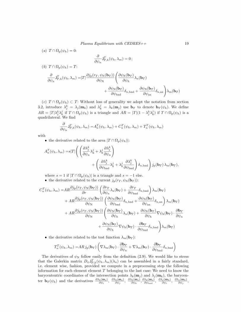
Plasma Equilibrium with CEDRES++ 19
(a) T ∩ Ωp(ψh) = 0:
∂
∂ψnJTP,h(ψh, λm) = 0 ;
(b) T ∩ Ωp(ψh) = T :
∂
∂ψnJTP,h(ψh, λm) =|T |∂jp(rT , ψN(bT ))
∂ψN
(∂ψN(bT )
∂ψhλn(bT )
+∂ψN(bT )
∂ψbndδn,bnd +
∂ψN(bT )
∂ψaxδn,ax
)λm(bT )
(c) T ∩ Ωp(ψh) ⊂ T : Without loss of generality we adopt the notation from section
3.2, introduce λkj = λj(mk) and λjk = λk(mj) use bT to denote bT (ψh). We define
AR = |T |λkjλjk if T ∩ Ωp(ψh) is a triangle and AR = |T |(1 − λkjλ
jk) if T ∩ Ωp(ψh) is a
quadrilateral. We find
∂
∂ψnJTP,h(ψh, λm) =ATn (ψh, λm) + CTn (ψh, λm) + TTn (ψh, λm)
with• the derivative related to the area |T ∩ Ωp(ψh)|:
ATn (ψh, λm) =s|T |
((∂λkj∂ψn
λjk + λjk∂λkj∂ψn
)
+
(∂λkj∂ψbnd
λjk + λjk∂λkj∂ψbnd
)δn,bnd
)jp(bT )λm(bT ),
where s = 1 if |T ∩ Ωp(ψh)| is a triangle and s = −1 else.• the derivative related to the current jp(rT , ψN(bT )):
CTn (ψh, λm) =AR∂jp(rT , ψN(bT ))
∂r
(∂rT∂ψn
λn(bT ) +∂rT∂ψbnd
δn,bnd
)λm(bT )
+AR∂jp(rT , ψN(bT ))
∂ψN
(∂ψN(bT )
∂ψbndδn,bnd +
∂ψN(bT )
∂ψaxδn,ax
)λm(bT )
+AR∂jp(rT , ψN(bT ))
∂ψN
(∂ψN(bT )
∂ψhλn(bT ) +
∂ψN(bT )
∂ψh∇ψh(bT ) · ∂bT
∂ψn
+∂ψN(bT )
∂ψh∇ψh(bT ) · ∂bT
∂ψbndδn,bnd
)λm(bT )
• the derivative related to the test function λm(bT ):
TTn (ψh, λm) =ARjp(bT )
(∇λm(bT ) · ∂bT
∂ψn+∇λm(bT ) · ∂bT
∂ψbndδn,bnd
)The derivatives of ψN follow easily from the definition (2.9). We would like to stress
that the Galerkin matrix DψJTP,h(ψh, λm)(λn) can be assembled in a fairly standard,
i.e. element wise, fashion, provided we compute in a preprocessing step the followinginformation for each element element T belonging to the last case: We need to know thebarycententric coordinates of the intersection points λk(mj) and λj(mk), the barycen-
ter bT (ψh) and the derivatives∂λk(mj)∂ψi
,∂λk(mj)∂ψj
,∂λk(mj)∂ψk
,∂λk(mj)∂ψbnd
,∂λj(mk)∂ψi
,∂λj(mk)∂ψj
,

20 H. Heumann et. al.
∂λj(mk)∂ψk
,∂λj(mk)∂ψbnd
and ∂bT∂ψi
, ∂bT∂ψj
, ∂bT∂ψk
, ∂bT∂ψbnd. All this information can be easily computed
for given ψh, ψbnd and ψax using the formulas (3.14), (3.15) and (3.17). All the termsthat contain the Kronecker deltas δn,bnd or δn,ax lead to non-local entries in the stiffnessmatrix. They connect the coefficients ψi1 = ψbnd and ψi2 = ψax with all coefficients ψjthat are associated to vertices of elements that are intersected by the plasma domainΩP(ψh).
The size of the algebraic systems that we need to solve in each iteration correspondsto the number of vertices of the triangulation. Even for very fine discretizations it istoday possible to use direct linear solvers such as UMFPACK (Davis 2011). As long asthe storage amount for the algebraic system does not exceed the memory, modern directsolvers will outperform in most cases an iterative solver.
3.4. Sequential Quadratic Programming for the Inverse Problems
In CEDRES++ we use the following fully discrete reformulation of the inverse Problems3 and 4, to find optimal currents in the poloidal field coils.
Inverse Problem 17 (Static). Let Sp′ : [0, 1] → R and Sff ′ : [0, 1] → R be twoknown functions. We set p′(ψ) = Sp′(ψN) and ff ′(ψ) = Sff ′(ψN) in (3.2). We solve thefollowing minimization problem:
minψh,I1,1,...IL,NL
K(ψh) +R(I1,1, . . . IL,NL) subject to (3.19) . (3.28)
Inverse Problem 18 (Static, with given plasma current IP). Let Sp′ : [0, 1]→R and Sff ′ : [0, 1] → R be two known functions and assume additionally that the totalplasma current IP is given. We set p′(ψ) = Sp′(ψN) and ff ′(ψ) = Sff ′(ψN) in (3.2).We solve the following minimization problem:
minλ,ψh,I1,1,...IL,NL
K(ψh) +R(I1,1, . . . IL,NL) subject to (3.20). (3.29)
The inverse Problems 17 and 18 are finite dimensional constrained optimization prob-lems. The sequential quadratic programming (SQP) method is the fastest method forfinite dimensional constrained optimization problems. We refer to the text book (No-cedal & Wright 2006, Chapter 18) for the details and explain here only the basic idea.
Both inverse Problems 17 and 18 are optimization problems of the following type
minu,y
1
2yTKy +
1
2uTHu s.t B(y) = F (u), (3.30)
where the quadratic matrices H and K are the discretization of the cost functions Kand R, the state variable y is the vector of the finite element coefficients ψi and thescaling factor λ, the control variable u is the vector of the N currents Ii in the poloidalfield coils and B and F the Galerkin discretizations of (3.19) or (3.20). The Lagrangefunction formalism in combination with Newton-type iterations is one approach to derivethe SQP-methods: the Lagrangian for (3.30) is
L(y,u,p) =1
2yTKy +
1
2uTHu + pT (B(y)− F (u)) (3.31)
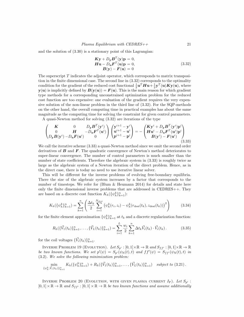
Plasma Equilibrium with CEDRES++ 21
and the solution of (3.30) is a stationary point of this Lagrangian:
Ky +DyBT (y)p = 0,
Hu−DuFT (u)p = 0,
B(y)− F (u) = 0
(3.32)
The superscript T indicates the adjoint operator, which corresponds to matrix transposi-tion in the finite dimensional case. The second line in (3.32) corresponds to the optimalitycondition for the gradient of the reduced cost functional 1
2uTHu+ 12yT (u)Ky(u), where
y(u) is implicitly defined by B(y(u)) = F (u). This is the main reason for which gradienttype methods for a corresponding unconstrained optimization problem for the reducedcost function are too expensive: one evaluation of the gradient requires the very expen-sive solution of the non-linear problem in the third line of (3.32). For the SQP-methodson the other hand, the overall computing time in practical examples has about the samemagnitude as the computing time for solving the constraint for given control parameters.
A quasi-Newton method for solving (3.32) are iterations of the type K 0 DyBT (yi)
0 H −DuFT (ui)
DyB(yi)−DuF (ui) 0
yi+1 − yi
ui+1 − ui
pi+1 − pi
= −
Kyi +DyBT (yi)pi
Hui −DuFT (ui)pi
B(yi)− F (ui)
(3.33)
We call the iterative scheme (3.33) a quasi-Newton method since we omit the second orderderivatives of B and F . The quadratic convergence of Newton’s method deteriorates tosuper-linear convergence. The number of control parameters is much smaller than thenumber of state coefficients. Therefore the algebraic system in (3.33) is roughly twice aslarge as the algebraic system of a Newton iteration of the direct problem. Hence, as inthe direct case, there is today no need to use iterative linear solver.
This will be different for the inverse problems of evolving free-boundary equilibria.There the size of the algebraic system increases by a factor that corresponds to thenumber of timesteps. We refer for (Blum & Heumann 2014) for details and state hereonly the finite dimensional inverse problems that are addressed in CEDRES++. Theyare based on a discrete cost function Kh(ψkhnk=1):
Kh(ψkhnk=1) =
n∑k=1
(∆tk
2
Ndesi∑i=1
(ψkh(ri, zi)− ψkh(rdesi(tk), zdesi(tk))
)2)(3.34)
for the finite element approximation ψkhnk=1 at tk and a discrete regularization function:
Rh(~V1(tk)nk=1, . . . , ~VL(tk)nk=1) =
L∑i=1
wi2
n∑k=1
∆tk~Vi(tk) · ~Vi(tk) . (3.35)
for the coil voltages ~Vi(tk)nk=1.
Inverse Problem 19 (Evolution). Let Sp′ : [0, 1]×R→ R and Sff ′ : [0, 1]×R→ Rbe two known functions. We set p′(ψ) = Sp′(ψN(t), t) and ff ′(ψ) = Sff ′(ψN(t), t) in(3.2). We solve the following minimization problem:
minψkh,~Vi(tk)nk=1
Kh(ψkhnk=1) +Rh(~V1(tk)nk=1, . . . , ~VL(tk)nk=1) subject to (3.21) .
Inverse Problem 20 (Evolution, with given plasma current IP). Let Sp′ :[0, 1]×R→ R and Sff ′ : [0, 1]×R→ R be two known functions and assume additionally

22 H. Heumann et. al.
that the total plasma current IP is given. We set p′(ψ) = Sp′(ψN(t), t) and ff ′(ψ) =Sff ′(ψN(t), t) in (3.2). We solve the following minimization problem:
minλk,ψkh,~Vi(tk)nk=1
Kh(ψkhnk=1) +Rh(~V1(tk)nk=1, . . . , ~VL(tk)nk=1) subject to (3.22) .
We would like to highlight that the SQP-method relies on proper derivatives of the non-linear operators B and F . In our case F is affine, hence the derivative of B remains themost difficult part. On the other hand these derivatives are exactly the same derivativesthat we used for the new Newton methods. Hence the implementation of a SQP-methodfor the inverse problem uses the same main building blocks.
3.5. Flux Surface Averages and Geometric Coefficients
As for any equilibrium code numerous outputs can be extracted from the poloidal fluxmap computed. These include purely geometric information on the plasma shape (plasmaboundary, geometric axis, elongation . . . ), global parameters (such as total plasma cur-rent IP, poloidal beta βp, internal inductance li, . . . ), 1D profiles of quantities constanton flux isolines in the plasma and 2D maps (ψ itself but also Br, Bz, jp, . . . ). All theseoutputs are standardized and follow the conventions of the European Integrated TokamakModelling Project (Falchetto et al. 2014; ITM 2013). We are not going to detail all ofthem in this paper. Let us however give some details on the computation of some of theimportant 1D profiles in the plasma. For ψN ∈ [0, 1], Sf (ψN) = f(ψ) is computed byintegration of Sff ′
Sf (ψN) = [(r0B0)2 − 2(ψbnd − ψax)
∫ 1
ψN
Sff ′(x)dx]1/2, (3.36)
where B0 is the vacuum toroidal field at r = r0. Let us define a discretization of the unitinterval [0, 1] by S + 1 values ψ0
N = 0, . . . , ψSN = 1. These points are taken as abscissa forall computed 1D profiles. For each ψsN the contour line ΓψsN is extracted from the finite
element representation of the solution as a list of Ns segments between mls,1 = (rls,1, z
ls,1)
and mls,2 = (rls,2, z
ls,2) with length |Lls|, for l = 1 to Ns.
The toroidal flux coordinate is defined as ρ(ψN) =√φ(ψN)/πB0 where φ(ψN) =∫
ΩψN
f(ψ(r,z))r drdz and ΩψN is the domain bounded by the line of flux ΓψN
. The quantities
φs and ρs are computed from the discrete ψh for all ψsN using a barycentric quadraturerule (cf. Section 3.2):
φs =∑T
Sf (ψN(bT (ψh)))
rT (ψh)|T ∩ ΩψsN |. (3.37)
The profiles ψs and ρs being known one can compute (∂ψ∂ρ )s = ψ′s using finite differences.In the same way the volume profile is computed as
V ols = 2π∑T
rT (ψh)|T ∩ ΩψsN | (3.38)
and (∂V ol∂ρ )s = V ol′s using finite differences.
Following (Blum 1987) the average of a quantity A over magnetic surfaces can becomputed as
〈A〉s = (
∫Γψs
N
Ar
|∇ψh|dl)/(
∫Γψs
N
r
|∇ψh|dl). (3.39)

Plasma Equilibrium with CEDRES++ 23
A number of 1D profiles, also called geometric coefficients, are computed as such averages,e.g. 〈1/r2〉 or 〈|∇ρ|2/r2〉 . The integrals over flux contour lines involved are approximatedas follows: ∫
ΓψsN
Ar
|∇ψh|dl ≈
Ns∑l=1
1
2
(rls,1A(ml
s,1)
|∇ψh|T ls |+rls,2A(ml
s,2)
|∇ψh|T ls |
)|Lls|. (3.40)
where T ls is the triangle which is intersected by the segment between mls,1 and ml
s,2 and
mls,· = (rls,·, z
ls,·) . |∇ψh|T ls | is constant in the triangle and computed from the 3 values
at the nodes of T ls.
3.6. Volume integrated Poynting theorems
The subset of equations (2.1) and (2.2) we used in section 2 to derive the evolutionproblems 5 and 6 that are solved in CEDRES++ involve the poloidal Faraday and thetoroidal Ampere law. Hence, the poloidal Poynting theorem (2.4) can be used to checkthe accuracy of the solution independently of an additional treatment of the transportequations.
We integrate the poloidal Poynting theorem (2.4) over a volume V ol that contains allthe plasma of a given scenario and get, by toroidal symmetry:∫∂S
∇ψ · nµ0r
∂tψds = −∫S∩ΩP(ψ)
(rp′(ψ) +
1
µ0rff ′(ψ)
)∂tψdrdz +
∫S
∇ψ · ∇∂tψµ0r
drdz,
(3.41)where S denotes the intersection of V ol with the poloidal plane.
If we choose S to be the domain of the plasma ΩP(ψ) then the left hand side of equation(3.41) is VloopIP, where Vloop is the plasma loop voltage. The first integral of the righthand side is related to the time rate of variation of the toroidal magnetic energy and tothe work done against the plasma pressure gradient. The last term of the righthand sideis the time rate of variation of the poloidal magnetic field energy.
We would like to stress that the integrated poloidal Poynting theorem correspondsto a variational formulation of the Grad-Shafranov-Schluter equations on S. Using thenotation (3.2) of our variational formulation from Section 3 we remark that the twointegrals on the righthand side correspond to Jp(ψ, χS∂tψ) and A(ψ, χS∂tψ), where χSis the characteristic function of S. Hence, it can be shown that the solutions ψk of theevolution problems 15 and 16 fulfill the volume integrated Poynting theorem up to firstorder accuracy in the mesh size.
The volume integrated version of the toroidal Poynting theorem (2.3) together with thestatic inverse mode was used in (Ane et al. 2000) for the optimization of ITER scenarios.
4. Tests and Examples
4.1. Validation and Performance
From the best of our knowledge, there does not exist analytical solutions for the freeboundary equilibrium problem considered in this paper. To provide nevertheless someevidence for convergence of the method, we follow a common approach in engineeringand study the convergence towards a numerical solution that is computed on a very finemesh.
We consider a static equilibrium with a given plasma current (Problem 2) in ITERgeometry. The plasma current is Ip = 15.10 × 10⁶A and the current density profile isprescribed using the model (2.11) with r0 = 6.2m α = 0.5978, β = 0.5978, γ = 1.395.
24 H. Heumann et. al.
0 5 10 15 20 25
−15
−10
−5
0
5
10
15
R (m)
Z (
m)
ψ isofluxVacuum vesselCoils I>0Coils I<0Passive structuresIronPlasma boundaryMagnetic axisX−point
4 5 6 7 8 9 10 11
−4
−3
−2
−1
0
1
2
3
4
R (m)
Z(m
)
ψ isofluxVacuum vessel
Plasma boundaryMagnetic axisisoflux ψ
n = 0.95
X−pointContact plasma−limiter
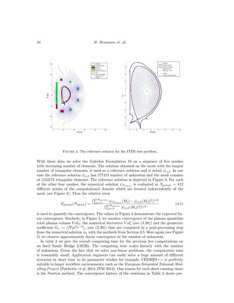
Figure 3. The reference solution for the ITER test problem.
With these data we solve the Galerkin Formulation 16 on a sequence of five mesheswith increasing number of elements. The solution obtained on the mesh with the largestnumber of triangular elements, is used as a reference solution and is noted ψref . In ourcase the reference solution ψref has 577415 number of unknowns and the mesh consistsof 1153174 triangular elements. The reference solution is depicted in Figure 3. For eachof the other four meshes, the numerical solution ψNukwn is evaluated at Npoints = 812different points of the computational domain which are located independently of themesh (see Figure 4). Then the relative error
Epoints(Nukwn) =(∑Npointsi=1 |ψNukwn(Mi)− ψref (Mi)|2)1/2
(∑Npointsi=1 |ψref (Mi)|2)1/2
(4.1)
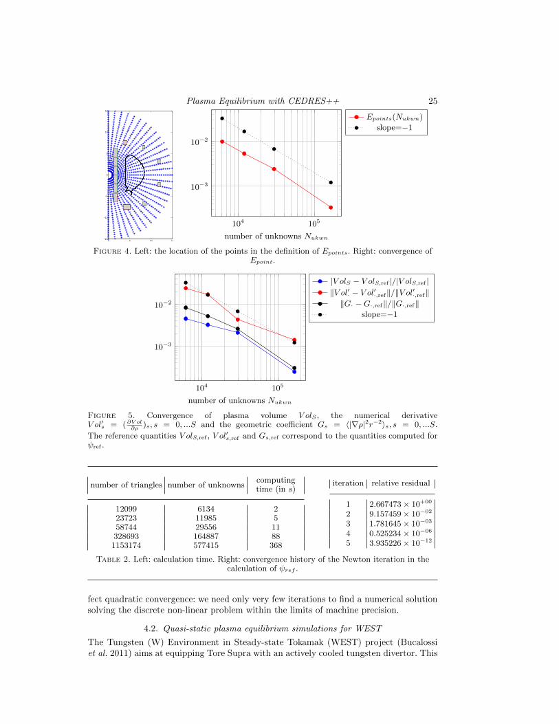
is used to quantify the convergence. The values in Figure 4 demonstrate the expected lin-ear convergence. Similarly, in Figure 5, we monitor convergence of the plasma quantitiestotal plasma volume V olS , the numerical derivative V ol′s (see (3.38)) and the geometriccoefficient Gs := 〈|∇ρ|2r−2〉s (see (3.39)) that are computed in a post-processing stepfrom the numerical solution ψh with the methods from Section 3.5. Here again (see Figure5) we observe approximately linear convergence in the number of unknowns.
In table 2 we give the overall computing time for the previous five computations onan Intel Sandy Bridge 2.6GHz. The computing time scales linearly with the numberof unknowns. Given the fact that we solve non-linear problems, the computation timeis reasonably small. Application engineers can easily solve a huge amount of differentscenarios in short time to do parameter studies for example. CEDRES++ is perfectlysuitable in larger workflow environments, such as the European Integrated Tokamak Mod-elling Project (Falchetto et al. 2014; ITM 2013). One reason for such short running timesis the Newton method. The convergence history of the residuum in Table 2 shows per-
Plasma Equilibrium with CEDRES++ 25
0 5 10 15−15
−10
−5
0
5
10
15
104 105
10−3
10−2
number of unknowns Nukwn
Epoints(Nukwn)
slope=−1
Figure 4. Left: the location of the points in the definition of Epoints. Right: convergence ofEpoint.
104 105
10−3
10−2
number of unknowns Nukwn
|V olS − V olS,ref |/|V olS,ref |‖V ol′· − V ol′·,ref‖/‖V ol′·,ref‖‖G· −G·,ref‖/‖G·,ref‖
slope=−1
Figure 5. Convergence of plasma volume V olS , the numerical derivativeV ol′s = ( ∂V ol
∂ρ)s, s = 0, ...S and the geometric coefficient Gs = 〈|∇ρ|2r−2〉s, s = 0, ...S.
The reference quantities V olS,ref , V ol′s,ref and Gs,ref correspond to the quantities computed for
ψref .
number of triangles number of unknownscomputingtime (in s)
12099 6134 223723 11985 558744 29556 11328693 164887 881153174 577415 368
iteration relative residual
1 2.667473× 10+00
2 9.157459× 10−02
3 1.781645× 10−03
4 0.525234× 10−06
5 3.935226× 10⁻¹²
Table 2. Left: calculation time. Right: convergence history of the Newton iteration in thecalculation of ψref .
fect quadratic convergence: we need only very few iterations to find a numerical solutionsolving the discrete non-linear problem within the limits of machine precision.
4.2. Quasi-static plasma equilibrium simulations for WEST
The Tungsten (W) Environment in Steady-state Tokamak (WEST) project (Bucalossiet al. 2011) aims at equipping Tore Supra with an actively cooled tungsten divertor. This

26 H. Heumann et. al.
|Bpol| |Hpol| |Bpol| |Hpol|
1 0.00 0 9 1.76 7.968× 10³
2 0.50 3.833× 10² 10 2.06 4.821× 10⁴
3 0.70 3.982× 10² 11 2.25 1.628× 10⁵
4 0.80 4.102× 10² 12 3.05 8.090× 10⁵
5 0.88 4.270× 10² 13 4.05 1.588× 10⁶
6 1.00 4.703× 10² 14 6.05 3.178× 10⁶
7 1.20 6.274× 10² 15 98.20 7.651× 10⁷
8 1.52 2.474× 10³ 16 105 7.957× 10¹⁰
Table 3. The data for the poloidal magnetic field |Bpol| and the poloidal magnetizing field|Hpol| that is used to reconstruct the magnetic permeability.
represents a major change in the magnetic configuration of Tore Supra, moving from acircular limited configuration to a diverted (or X-point) configuration. CEDRES++ isone of the main modeling tools used for the preparation of WEST. It has been employed inparticular for the definition of reference equilibria, the dimensioning of the plasma verticalposition feedback system, the design of the plasma shape controller, breakdown studies,disruption simulations, etc. We give below a few examples of CEDRES++ simulationsfor WEST. Note that Tore Supra is an iron core tokamak and that the iron is taken intoaccount in all of these simulations. The six return arms of the iron core are representedin CEDRES++ by an axisymmetric equivalent model, which gives the 1/R shape of thereturn arms visible in Figure 6. We are using the experimental data for the poloidalmagnetic field Bpol and the poloidal magnetizing field Hpol from table 3, do piecewiselinear interpolation of these data and reconstruct the permeability for arbitrary magneticfield values via µFE(B2
pol) = |Bpol||Hpol|−1.We present in the following sections three different examples from research for WEST
that use the static direct, static evolution and inverse static modes of CEDRES++. Firstsimulations with the inverse evolution mode are presented in (Blum & Heumann 2014).The inverse static mode of CEDRES++ is also extremely useful in order to define andoptimize reference equilibria. We will give details for WEST in a forthcoming publication.
4.2.1. The current-focused case: direct static mode
Figure 6 shows a typical WEST poloidal flux map calculated by CEDRES++ incurrent-focused mode. The X-point is visible at the bottom of the plasma. Here, CE-DRES++ solves the direct static Problem 2 with prescribed total plasma current IP =700kA and with the parametrized current profiles Sp′ and Sff ′ in (2.11), using α = 1,β = 1.5, γ = 0.9, r0 = 2.6m. The vacuum toroidal field is B0 = 3.524T at r = 2.6m. Afew output parameters are: βp = 1.70, li = 0.93, q95 = 3.33, q0 = 1.17.
4.2.2. The voltage-evolution-focused case, direct evolution mode
Starting from the equilibrium in the previous section, we run CEDRES++ in directevolution mode to solve problem 6. We keep all the input parameters fixed and we applya constant voltage to the coils, equal to the resistive voltage being the product of coilresistance and current, except for the divertor coils, where we perturb the resistive voltagewith ∆V = +0.1V olt in the lower coil and ∆V = −0.1V olt in the upper coil. This isin order to trigger a vertical instability (otherwise the plasma would stay in place). Thesimulation is run with a time step of 20ms. Figure 7 shows the plasma boundary at
Plasma Equilibrium with CEDRES++ 27
0 2 4
−3
−2
−1
0
1
2
3
R (m)
Z (
m)
1.5 2 2.5 3−1
−0.5
0
0.5
1
R (m)
Z (
m)
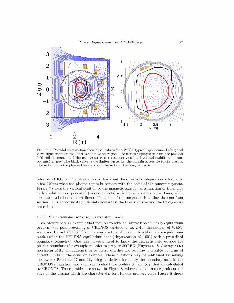
Figure 6. Poloidal cross section showing ψ-isolines for a WEST typical equilibrium. Left: globalview; right: zoom on the inner vacuum vessel region. The iron is displayed in blue, the poloidalfield coils in orange and the passive structures (vacuum vessel and vertical stabilization com-ponents) in grey. The black curve is the limiter curve, i.e. the domain accessible to the plasma.The red curve is the plasma boundary and the red star the magnetic axis.
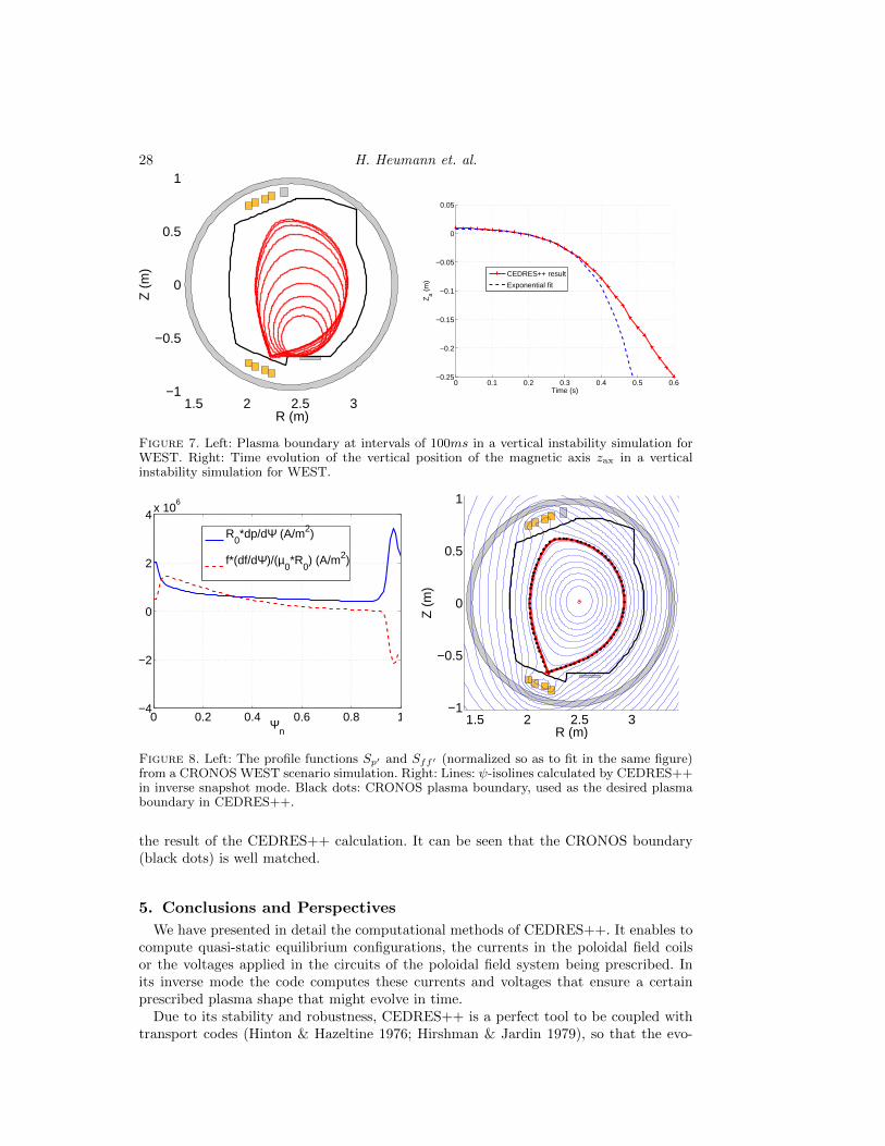
intervals of 100ms. The plasma moves down and the diverted configuration is lost aftera few 100ms when the plasma comes in contact with the baffle of the pumping system.Figure 7 shows the vertical position of the magnetic axis zax as a function of time. Theearly evolution is exponential (as one expects) with a time constant τz = 95ms, whilethe later evolution is rather linear. The error of the integrated Poynting theorem fromsection 3.6 is approximately 5% and decreases if the time step size and the triangle sizeare refined.
4.2.3. The current-focused case, inverse static mode
We present here an example that requires to solve an inverse free-boundary equilibriumproblem: the post-processing of CRONOS (Artaud et al. 2010) simulations of WESTscenarios. Indeed, CRONOS simulations are typically run in fixed-boundary equilibriummode (using the HELENA equilibrium code (Huysmans et al. 1991) with a prescribedboundary geometry). One may however need to know the magnetic field outside theplasma boundary (for example in order to prepare JOREK (Huysmans & Czarny 2007)non-linear MHD simulations), or to assess whether the scenario is feasible in terms ofcurrent limits in the coils for example. These questions may be addressed by solvingthe inverse Problems 17 and 18, using as desired boundary the boundary used in theCRONOS simulation, and as current profile those profiles Sp′ and Sff ′ that are calculatedby CRONOS. These profiles are shown in Figure 8, where one can notice peaks at theedge of the plasma which are characteristic for H-mode profiles, while Figure 8 shows
28 H. Heumann et. al.
1.5 2 2.5 3−1
−0.5
0
0.5
1
R (m)
Z (
m)
0 0.1 0.2 0.3 0.4 0.5 0.6−0.25
−0.2
−0.15
−0.1
−0.05
0
0.05
Time (s)
Za (
m)
CEDRES++ result
Exponential fit
Figure 7. Left: Plasma boundary at intervals of 100ms in a vertical instability simulation forWEST. Right: Time evolution of the vertical position of the magnetic axis zax in a verticalinstability simulation for WEST.
0 0.2 0.4 0.6 0.8 1−4
−2
0
2
4x 10
6
Ψn
R0*dp/dΨ (A/m2)
f*(df/dΨ)/(µ0*R
0) (A/m2)
1.5 2 2.5 3−1
−0.5
0
0.5
1
R (m)
Z (
m)
Figure 8. Left: The profile functions Sp′ and Sff ′ (normalized so as to fit in the same figure)from a CRONOS WEST scenario simulation. Right: Lines: ψ-isolines calculated by CEDRES++in inverse snapshot mode. Black dots: CRONOS plasma boundary, used as the desired plasmaboundary in CEDRES++.
the result of the CEDRES++ calculation. It can be seen that the CRONOS boundary(black dots) is well matched.
5. Conclusions and Perspectives
We have presented in detail the computational methods of CEDRES++. It enables tocompute quasi-static equilibrium configurations, the currents in the poloidal field coilsor the voltages applied in the circuits of the poloidal field system being prescribed. Inits inverse mode the code computes these currents and voltages that ensure a certainprescribed plasma shape that might evolve in time.
Due to its stability and robustness, CEDRES++ is a perfect tool to be coupled withtransport codes (Hinton & Hazeltine 1976; Hirshman & Jardin 1979), so that the evo-

Plasma Equilibrium with CEDRES++ 29
lution of plasma equilibrium is simulated at the resistive timescale consistently withtransport processes. Reciprocally the transport codes take into account the precise ge-ometry of the magnetic flux lines. The numerical stability of such a coupling is challengingand subject of ongoing research. This is particularly important for the simulation andoptimization of scenarios in new generation tokamaks. CEDRES++, when coupled tothe transport codes CRONOS (Artaud et al. 2010) and ETS (Coster et al. 2010), is inuse for simulating such self consistent plasma evolution. The evolution mode itself, whenplasma current profiles are given, is a good practical approach for vertical stability stud-ies where the timescale of interest is much shorter than the current diffusion timescaleof the plasma.
Furthermore, the modular and clear structure of CEDRES++ and the emphasis onaccurate Newton methods, will make CEDRES++ very useful to implement fully auto-matic approaches to the optimization of scenarios. It will be easy to study and predictoperational limits, and to devise control strategies that circumvent such limits.
It is possible to extend the methods presented in this work to higher order finiteelements. Nevertheless, there are a couple of obstacles in order to obtain entirely higherorder accurate methods:
• We are solving here a non-linear elliptic problem with discontinuous coefficients (inthe case of iron-transformer tokamaks) and discontinuous righthand side. The standardconvergence theory for finite elements and elliptic regularity theory does not yield im-proved approximation results for polynomials of degree higher than 1. Nevertheless prac-tical experience and the theoretical results in (Feistauer & Sobotkov 1990) for low-orderapproximation of non-linear problems and in (Li et al. 2010) for high-order approxi-mation of linear problems suggest improved accuracy. From the regularity theory formagneto-statics, we know in the case of iron-transformer tokamaks (such as JET or ToreSupra) that the solution lacks of regularity in the vicinity of the iron parts, in particularclose to the interfaces air/iron and the corners of subdomains with iron. In such non-regular settings, it is required to switch to the so-called hp-version of the finite elementmethod (Schwab 2004), that uses small triangles and low order polynomials in regionswith non-regular solution and large triangles and high order polynomials elsewhere.• Moreover, the general setting suffers from a fairly large modeling error due to the
experimental permeability curve and to the axisymmetric representation of the ferro-magnetic circuit that in reality consists of an iron core and a certain number of non-axisymmetric return limbs. It is not clear whether such modeling errors might surpassthe discretization error.• Higher order accuracy requires also sufficiently accurate quadrature rules in the defi-
nition of the Galerkin methods. While such higher order quadrature rules are standard for(iso-parametric) finite elements, we foresee technical difficulties alongside with a consid-erable increase of computational complexity for the integrals over the intersection of theplasma with triangles. We need to implement sufficiently accurate quadrature rules forpolygonal domains with non-straight boundaries. On top of this, we need to implementfor the Newton method the derivatives of such quadrature rules.
We are planning to investigate such topics in the near future and to compare with al-ternative approaches. One promising alternative might be to switch after a couple ofNewton iterations to a different discretization scheme that uses separate meshes andseparate polynomial degrees for the representation of the flux in the plasma domain andits exterior. The non-linear coupling of the plasma and its exterior will lead to iterationschemes that induce small variations of the two meshes from one iteration to the next.With this, both the location of the magnetic axis and X-point are a priori not limited

30 H. Heumann et. al.
to a finite set of points, as it is the case for linear Lagrangian elements with fixed globalmesh.
Any higher order method will involve more sophisticated algorithms and it is hardto predict if the accuracy at a fixed computing time will drastically improve. If highaccuracy is required at the moment, this can still be achieved with reasonable effort bysimple mesh refinement. The running time of the current version of the code is not yetoptimized and still it is possible to do calculations with over half a million unknowns inless than 7 minutes on a workstation.
6. Acknowledgments
This work, supported by the European Communities under the contract of Associationbetween EURATOM-CEA was carried out within the framework of the Task Force onIntegrated Tokamak Modelling of the European Fusion Development Agreement. Theviews and opinions expressed herein do not necessarily reflect those of the EuropeanCommission.
The authors would like to thank the reviewers for their comments that help improvethe manuscript.
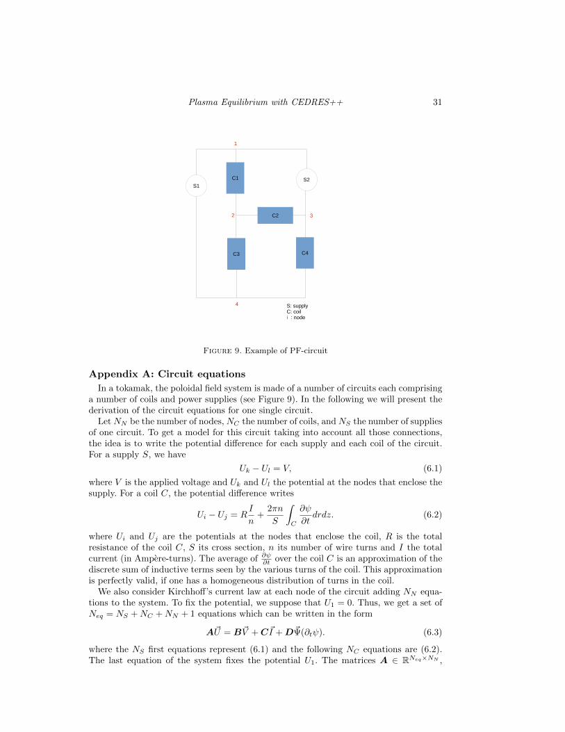
Plasma Equilibrium with CEDRES++ 31
C1
C3
C2
S1S2
1
2 3
4 S: supplyC: coili : node
C3 C4
Figure 9. Example of PF-circuit
Appendix A: Circuit equations
In a tokamak, the poloidal field system is made of a number of circuits each comprisinga number of coils and power supplies (see Figure 9). In the following we will present thederivation of the circuit equations for one single circuit.
Let NN be the number of nodes, NC the number of coils, and NS the number of suppliesof one circuit. To get a model for this circuit taking into account all those connections,the idea is to write the potential difference for each supply and each coil of the circuit.For a supply S, we have
Uk − Ul = V, (6.1)
where V is the applied voltage and Uk and Ul the potential at the nodes that enclose thesupply. For a coil C, the potential difference writes
Ui − Uj = RI
n+
2πn
S
∫C
∂ψ
∂tdrdz. (6.2)
where Ui and Uj are the potentials at the nodes that enclose the coil, R is the totalresistance of the coil C, S its cross section, n its number of wire turns and I the totalcurrent (in Ampere-turns). The average of ∂ψ∂t over the coil C is an approximation of thediscrete sum of inductive terms seen by the various turns of the coil. This approximationis perfectly valid, if one has a homogeneous distribution of turns in the coil.
We also consider Kirchhoff’s current law at each node of the circuit adding NN equa-tions to the system. To fix the potential, we suppose that U1 = 0. Thus, we get a set ofNeq = NS +NC +NN + 1 equations which can be written in the form
A~U = B~V + C~I + D~Ψ(∂tψ). (6.3)
where the NS first equations represent (6.1) and the following NC equations are (6.2).The last equation of the system fixes the potential U1. The matrices A ∈ RNeq×NN ,

32 H. Heumann et. al.
B ∈ RNeq×NS , C ∈ RNeq×(NS+NC) and D ∈ RNeq×NC are called potential matrix,voltage matrix, current matrix and induction matrix, respectively. The vectors ~U ∈ RNN ,~V ∈ RNS and ~I ∈ RNS+NC contain the electric potential at the circuit nodes, the voltagesapplied at the supplies and currents at the coils and the supplies. The components of thevector ~Ψ(∂tψ) ∈ RNC are the integrals
∫C∂tψdrdz over the domain that is occupied by
a coil C of the circuit.For given ~V , ~I and ~Ψ(∂tψ), there is a unique ~U which satisfies (6.3), hence ATA is
regular. We find
~U = (ATA)−1ATB~V + (ATA)−1ATC~I + (ATA)−1ATD~Ψ(∂tψ), (6.4)
plug this into (6.3) and get
E~I + F ~V + G~Ψ(∂tψ) = 0 , (6.5)
with
E = A(ATA)−1ATC −C
F = A(ATA)−1ATB −B
G = A(ATA)−1ATD −D.
The system (6.5) of Neq equations is over determined and ~I can be computed using thenormal equation
~I = S~V + R~Ψ(∂tψ) (6.6)
with S = −(ETE)−1ETF and R = −(ETE)−1ETG.

Plasma Equilibrium with CEDRES++ 33
REFERENCES
Albanese, R., Blum, J. & Barbieri, O. 1986 On the solution of the magnetic flux equation inan infinite domain. In EPS. 8th Europhysics Conference on Computing in Plasma Physics(1986).
Albanese, R., Blum, J. & De Barbieri, O. 1987 Numerical studies of the Next EuropeanTorus via the PROTEUS code. In 12th Conf. on Numerical Simulation of Plasmas, SanFrancisco.
Albanese, R. & Villone, F. 1998 The linearized create-l plasma response model for the controlof current, position and shape in tokamaks. Nuclear Fusion 38 (5), 723.
Ane, J.M., Grandgirard, V., Albajar, F. & Johner, J. 2000 Design of next step toka-mak: Consistent analysis of plasma performance flux composition and poloidal field sys-tem. In 18th IAEA Fusion Energy Conference, Sorrento, http: // www. iaea. org/ inis/collection/ NCLCollectionStore/ _Public/ 33/ 029/ 33029055. pdf .
Ariola, M. & Pironti, A. 2008 Magnetic Control of Tokamak Plasmas. Springer London.
Artaud, J.F., Basiuk, V., Imbeaux, F., Schneider, M., Garcia, J., Giruzzi, G., Huynh,P., Aniel, T., Albajar, F., Ane, J.M., Becoulet, A., Bourdelle, C., Casati, A.,Colas, L., Decker, J., Dumont, R., Eriksson, L.G., Garbet, X., Guirlet, R.,Hertout, P., Hoang, G.T., Houlberg, W., Huysmans, G., Joffrin, E., Kim, S.H.,Kchl, F., Lister, J., Litaudon, X., Maget, P., Masset, R., Pegourie, B., Peysson,Y., Thomas, P., Tsitrone, E. & Turco, F. 2010 The CRONOS suite of codes for inte-grated tokamak modelling. Nuclear Fusion 50 (4), 043001.
Bielak, J. & MacCamy, R. C. 1991 Symmetric finite element and boundary integral couplingmethods for fluid-solid interaction. Quart. Appl. Math. 49 (1), 107–119.
Blum, J. 1987 Numerical simulation of the plasma equilibrium in a tokamak . Wiley/Gauthier-Villars.
Blum, J., Boulbe, C. & Faugeras, B. 2012 Reconstruction of the equilibrium of the plasmain a tokamak and identification of the current density profile in real time. Journal ofComputational Physics 231 (3), 960 – 980.
Blum, J. & Heumann, H. 2014 Optimal control for quasi-static evolution of plasma equilibriumin tokamaks. Tech. Rep.. INRIA, Sophia Antipolis.
Blum, J., Le Foll, J. & Thooris, B. 1981 The self-consistent equilibrium and diffusion codeSCED. Computer Physics Communications 24, 235 – 254.
Bucalossi, J., Argouarch, A., Basiuk, V., Baulaigue, O., Bayetti, P., Bcoulet, M.,Bertrand, B., Brmond, S., Cara, P., Chantant, M., Corre, Y., Courtois, X., Do-ceul, L., Ekedahl, A., Faisse, F., Firdaouss, M., Garcia, J., Gargiulo, L., Gil, C.,Grisolia, C., Gunn, J., Hacquin, S., Hertout, P., Huysmans, G., Imbeaux, F., Jio-lat, G., Joanny, M., Jourd’heuil, L., Jouve, M., Kukushkin, A., Lipa, M., Lisgo,S., Loarer, T., Maget, P., Magne, R., Marandet, Y., Martinez, A., Mazon, D.,Meyer, O., Missirlian, M., Monier-Garbet, P., Moreau, P., Nardon, E., Panay-otis, S., Pgouri, B., Pitts, R.A., Portafaix, C., Richou, M., Sabot, R., Saille, A.,Saint-Laurent, F., Samaille, F., Simonin, A. & Tsitrone, E. 2011 Feasibility studyof an actively cooled tungsten divertor in tore supra for ITER technology testing. FusionEngineering and Design 86 (6-8), 684 – 688.
Chen, Goong & Zhou, Jianxin 1992 Boundary element methods. Academic Press, Ltd., Lon-don.
Ciarlet, P. G. 1978 The Finite Element Method for Elliptic Problems. Amsterdam: North-Holland Publishing Co., studies in Mathematics and its Applications, Vol. 4.
Cooper, W.A., Hirshman, S.P., Merkel, P., Graves, J.P., Kisslinger, J., Wobig,H.F.G., Narushima, Y., Okamura, S. & Watanabe, K.Y. 2009 Three-dimensionalanisotropic pressure free boundary equilibria. Computer Physics Communications 180 (9),1524 – 1533.
Costabel, M. & Stephan, E.P. 1990 Coupling of finite and boundary element methods foran elastoplastic interface problem. SIAM J. Numer. Anal. 27 (5), 1212–1226.
Coster, D.P., Basiuk, V., Pereverzev, G., Kalupin, D., Zagrksi, R., Stankiewicz, R.,Huynh, P. & Imbeaux, F. 2010 The european transport solver. Plasma Science, IEEETransactions on 38 (9), 2085–2092.
Davis, T.A. 2011 Umfpack http://www.cise.ufl.edu/research/sparse/umfpack/.

34 H. Heumann et. al.
Degtyarev, L.M. & Drozdov, V.V. 1985 An inverse variable technique in the MHD-equilibrium problem. Computer Physics Reports 2 (7), 341 – 387.
Degtyarev, L.M. & Drozdov, V.V. 1991 Adaptive mesh computation of magnetic hydrody-namic equilibrium. International Journal of Modern Physics C 02 (01), 30–38.
Delfour, M.C. & Zolesio, J.-P. 2011 Shapes and geometries, 2nd edn., Advances in Designand Control , vol. 22. Society for Industrial and Applied Mathematics (SIAM), Philadelphia,PA.
DeLucia, J., Jardin, S.C. & Todd, A.M.M. 1980 An iterative metric method for solving theinverse tokamak equilibrium problem. Journal of Computational Physics 37 (2), 183 – 204.
Falchetto, G.L., Coster, D., Coelho, R., Scott, B.D., Figini, L., Kalupin, D., Nar-don, E., Nowak, S., Alves, L.L., Artaud, J.F., Basiuk, V., Bizarro, Joo P.S.,Boulbe, C., Dinklage, A., Farina, D., Faugeras, B., Ferreira, J., Figueiredo,A., Huynh, Ph., Imbeaux, F., Ivanova-Stanik, I., Jonsson, T., Klingshirn, H.-J.,Konz, C., Kus, A., Marushchenko, N.B., Pereverzev, G., Owsiak, M., Poli, E.,Peysson, Y., Reimer, R., Signoret, J., Sauter, O., Stankiewicz, R., Strand, P.,Voitsekhovitch, I., Westerhof, E., Zok, T., Zwingmann, W., Contributors, ITM-TF, the ASDEX Upgrade Team & Contributors, JET-EFDA 2014 The EuropeanIntegrated Tokamak Modelling (ITM) effort: achievements and first physics results. NuclearFusion 54 (4), 043018.
Feistauer, Miloslav & Sobotkov, Veronika 1990 Finite element approximation of nonlin-ear elliptic problems with discontinuous coefficients. ESAIM: Mathematical Modelling andNumerical Analysis - Modlisation Mathmatique et Analyse Numrique 24 (4), 457–500.
Feneberg, W. & Lackner, K. 1973 Multipole tokamak equilibria. Nuclear Fusion 13 (4), 549.
Fitzgerald, M., Appel, L.C. & Hole, M.J. 2013 EFIT tokamak equilibria with toroidal flowand anisotropic pressure using the two-temperature guiding-centre plasma. Nuclear Fusion53 (11), 113040.
Freidberg, J. P. 1987 Ideal Magnetohydrodynamics. Plenum US.
Gatica, G.N. & Hsiao, G.C. 1995 The uncoupling of boundary integral and finite elementmethods for nonlinear boundary value problems. J. Math. Anal. Appl. 189 (2), 442–461.
Glowinski, R. & Marrocco, A. 1974 Analyse numerique du champ magnetique d’un alter-nateur par elements finis et sur-relaxation ponctuelle non lineaire. Comput. Methods Appl.Mech. Engrg. 3 (1), 55–85.
Goedbloed, J.P. & Lifschitz, A. 1997 Stationary symmetric magnetohydrodynamic flows.Physics of Plasmas (1994-present) 4 (10), 3544–3564.
Goedbloed, Johan P, Keppens, Rony & Poedts, Stefaan 2010 Advanced magnetohydro-dynamics: with applications to laboratory and astrophysical plasmas. Cambridge UniversityPress.
Goedbloed, Johan Peter & Poedts, Stefaan 2004 Principles of magnetohydrodynamics:with applications to laboratory and astrophysical plasmas. Cambridge university press.
Grad, H. 1967 Toroidal containment of a plasma. Physics of Fluids (1958-1988) 10 (1), 137–154.
Grad, H. & Rubin, H. 1958 Hydromagnetic equilibria and force-free fields. Proceedings of the2nd UN Conf. on the Peaceful Uses of Atomic Energy 31, 190.
Grandgirard, Virginie 1999 Modelisation de l’equilibre d’un plasma de tokamak. PhD thesis,l’Universite de Franche-Comte.
Gruber, R., Iacono, R. & Troyon, F. 1987 Computation of MHD equilibria by a quasi-inverse finite hybrid element approach. Journal of Computational Physics 73 (1), 168 –182.
Guazzotto, L., Betti, R., Manickam, J. & Kaye, S. 2004 Numerical study of tokamakequilibria with arbitrary flow. Physics of Plasmas (1994-present) 11 (2), 604–614.
Helton, F.J. & Wang, T.S. 1978 MHD equilibrium in non-circular tokamaks with field-shapingcoil systems. Nuclear Fusion 18 (11), 1523.
Hertout, P., Boulbe, C., Nardon, E., Blum, J., Bremond, S., Bucalossi, J., Faugeras,B., Grandgirard, V. & Moreau, P. 2011 The cedres++ equilibrium code and its ap-plication to ITER, JT-60SA and Tore Supra. Fusion Engineering and Design 86, 1045 –1048.
Plasma Equilibrium with CEDRES++ 35
Hinton, F.L. & Hazeltine, R.D. 1976 Theory of plasma transport in toroidal confinementsystems. Rev. Mod. Phys. 48, 239–308.
Hiptmair, R. 2003 Coupling of finite elements and boundary elements in electromagnetic scat-tering. SIAM J. Numer. Anal. 41 (3), 919–944.
Hirshman, S.P. & Betancourt, O. 1991 Preconditioned descent algorithm for rapid calcula-tions of magnetohydrodynamic equilibria. J. Comput. Phys. 96 (1), 99–109.
Hirshman, S. P. & Jardin, S. C. 1979 Two-dimensional transport of tokamak plasmas. Physicsof Fluids 22 (4), 731–742.
Hofmann, F. & Tonetti, G. 1988 Tokamak equilibrium reconstruction using Faraday rotationmeasurements. Nuclear Fusion 28 (10), 1871.
Huysmans, G.T.A. & Czarny, O. 2007 MHD stability in X-point geometry: simulation ofELMs. Nuclear Fusion 47 (7), 659.
Huysmans, G.T.A., Goedbloed, J.P. & Kerner, W. 1991 Isoparametric bicubic Hermiteelements for solution of the Grad–Shafranov equation. Proc. CP90 Conf. on Comp. Phys.p. 371.
ITM 2013 Integrated tokamak modelling. http://portal.efda-itm.eu/, integrated TokamakModelling.
Jardin, S.C. 2010 Computational methods in plasma physics. Boca Raton, FL : CRCPress/Taylor & Francis.
Jardin, S. C., Pomphrey, N. & DeLucia, J. 1986 Dynamic modeling of transport and posi-tional control of tokamaks. J. Comput. Phys. 66, 481–507.
Johnson, J.L., Dalhed, H.E., Greene, J.M., Grimm, R.C., Hsieh, Y.Y., Jardin, S.C.,Manickam, J., Okabayashi, M., Storer, R.G., Todd, A.M.M., Voss, D.E. &Weimer, K.E. 1979 Numerical determination of axisymmetric toroidal magnetohydro-dynamic equilibria. Journal of Computational Physics 32 (2), 212 – 234.
Lackner, K. 1976 Computation of ideal MHD equilibria. Computer Physics Communications12 (1), 33 – 44.
Lao, L.L., Ferron, J.R., Geoebner, R.J., Howl, W., St. John, H.E., Strait, E.J. &Taylor, T.S. 1990 Equilibrium analysis of current profiles in Tokamaks. Nuclear Fusion30 (6), 1035.
Lao, L.L., Hirshman, S.P. & Wieland, R.M. 1981 Variational moment solutions to theGrad–Shafranov equation. Physics of Fluids 24 (8), 1431–1440.
Lao, L.L., John, H. St., Stambaugh, R.D., Kellman, A.G. & Pfeiffer, W. 1985 Re-construction of current profile parameters and plasma shapes in tokamaks. Nuclear Fusion25 (11), 1611.
Li, Jingzhi, Melenk, Jens Markus, Wohlmuth, Barbara & Zou, Jun 2010 Optimal apriori estimates for higher order finite elements for elliptic interface problems. AppliedNumerical Mathematics 60 (1-2), 19 – 37.
Ling, K.M. & Jardin, S.C. 1985 The Princeton spectral equilibrium code: PSEC. Journal ofComputational Physics 58 (3), 300 – 335.
Lust, R. & Schluter, A. 1957 Axialsymmetrische magnetohydrodynamische Gleichgewicht-skonfigurationen. Z. Naturforsch. A 12, 850–854.
Luxon, J.L. & Brown, B.B. 1982 Magnetic analysis of non-circular cross-section tokamaks.Nuclear Fusion 22 (6), 813.
Maschke, E.K. & Perrin, H.J. 1984 An analytic solution of the stationary MHD equationsfor a rotating toroidal plasma. Physics Letters A 102 (3), 106 – 108.
Mc Carthy, P.J., Martin, P. & Schneider, W. 1999 The CLISTE Interpretive EquilibriumCode. Tech. Rep. IPP Report 5/85. Max-Planck-Institut fur Plasmaphysik.
Murat, F. & Simon, J. 1976 Sur le controle par un domaine geometrique. Tech. Rep. 76015.Laboratoire d’Analyse Numerique, Universite de Paris 6.
Nedelec, J.-C. 2001 Acoustic and electromagnetic equations, Applied Mathematical Sciences,vol. 144. Springer-Verlag, New York.
Nocedal, J. & Wright, S. J. 2006 Numerical optimization, 2nd edn. New York: Springer.Parail, V., Albanese, R., Ambrosino, R., Artaud, J.-F., Besseghir, K., Cavinato, M.,
Corrigan, G., Garcia, J., Garzotti, L., Gribov, Y., Imbeaux, F., Koechl, F.,Labate, C.V., Lister, J., Litaudon, X., Loarte, A., Maget, P., Mattei, M., Mc-Donald, D., Nardon, E., Saibene, G., Sartori, R. & Urban, J. 2013 Self-consistent
36 H. Heumann et. al.
simulation of plasma scenarios for iter using a combination of 1.5d transport codes andfree-boundary equilibrium codes. Nuclear Fusion 53 (11), 113002.
Park, W., Belova, E. V., Fu, G. Y., Tang, X. Z., Strauss, H. R. & Sugiyama, L. E.1999 Plasma simulation studies using multilevel physics models. Physics of Plasmas (1994-present) 6 (5), 1796–1803.
Pechstein, C. & Juttler, B. 2006 Monotonicity-preserving interproximation of B-H-curves.J. Comput. Appl. Math. 196 (1), 45–57.
Pustovitov, V.D. 2010 Anisotropic pressure effects on plasma equilibrium in toroidal systems.Plasma Physics and Controlled Fusion 52 (6), 065001.
Renard, Y. & Pommier, J. 2014 GetFEM++, an open-source finite element library. http://download.gna.org/getfem/html/homepage/index.html.
Schwab, C. 2004 p- and hp- finite element methods : theory and applications in solid and fluidmechanics. Oxford : Clarendon Press.
Shafranov, V.D. 1958 On magnetohydrodynamical equilibrium configurations. Soviet Journalof Experimental and Theoretical Physics 6, 545.
Shewchuk, J.R. 1996 Triangle: Engineering a 2D Quality Mesh Generator and Delaunay Trian-gulator. In Applied Computational Geometry: Towards Geometric Engineering (ed. Ming C.Lin & Dinesh Manocha), Lecture Notes in Computer Science, vol. 1148, pp. 203–222.Springer-Verlag, from the First ACM Workshop on Applied Computational Geometry.
Stephan, E.P. 1992 Coupling of finite elements and boundary elements for some nonlinearinterface problems. Comput. Methods Appl. Mech. Engrg. 101 (1-3), 61–72.
Turkington, B., Lifschitz, A., Eydeland, A. & Spruck, J. 1993 Multiconstrained vari-ational problems in magnetohydrodynamics: Equilibrium and slow evolution. Journal ofComputational Physics 106 (2), 269 – 285.
Wesson, J. 2004 Tokamaks. Oxford University Press.Zhao, K., Vouvakis, M.N. & Lee, J.-F. 2006 Solving electromagnetic problems using a novel
symmetric fem-bem approach. Magnetics, IEEE Transactions on 42 (4), 583–586.Zwingmann, W., Eriksson, L.-G. & Stubberfield, P. 2001 Equilibrium analysis of tokamak
discharges with anisotropic pressure. Plasma Physics and Controlled Fusion 43 (11), 1441.