Quantum ResistantCryptography

Antal Nemes

MSc. Mathematics

MSc. Thesis

Supervisor: Viktoria Villanyi

Department of Operations Research

Institutional Consultant: Peter Sziklai

Department of Computer Science

Eotvos Lorand University, Budapest

Faculty of Science

Budapest, 2012

Abstract

Among the many cryptographic schemes there are two groups of algorithms that

are widely used currently in applied cryptograpy: the algoritms which security is

based on the integer factorization problem and those based on the discrete logarithm

problem.

In the quantum computational model both these mathematical problems are

solvable in polynomial time, which leads to security questions when these algorithms

are applied.

In this thesis we will talk about the quantum computational model and discuss

some cryptographic schemes, which are considered to be resistant in the quantum

computational model.

A kvantum szamıtasi modellben nehany olyan eddig neheznek tartott problemara

sikerult polinomialis algoritmust talalni, melyekre titkosıtasi problemak alapulnak.

Igy azon algoritmusok, melyek biztonsagossaga ezen problemak nehezsegen ala-

pulnak, megbızhatosaguk megkerdojelezodott. Emiatt celszeru olyan titkosıtasi

semakat vizsgalni, melyek az alkalmazasokban eleg hatekonyak, mindemellett ellenallnak

a kvantum szamıtogepeknek is.

Ebben a szakdolgozatban bemutatjuk a kvantum szamıtasi modellt, majd targyalunk

nehany a kvantum szamıtogepeknek is ellenallo digitalis alaırasi semat illetve titkosıto

algoritmust.

Acknowledgements

I would like to thank my supervisor, Viktoria Villanyi for introducing me to this

exciting topic which hits many areas of science, such as quantum physics, functional

analyzis, algorithm theory, complexity theory and applied cryptography. I met a lot

of exciting and interesting theorems and concepts which motivated me to dive more

and more into the topic. I also want to thank her the interesting articles she gave

me, which was beneficial in writing the thesis, for her guidance, and for helping me

refining my thesis.

Contents

1 Introduction 6

2 Integer factorization, discrete logarithm 8

2.1 Integer factorization . . . . . . . . . . . . . . . . . . . . . . . . . . . 8

2.2 Discrete logarithm . . . . . . . . . . . . . . . . . . . . . . . . . . . . 9

3 Quantum computation 11

3.1 Physics . . . . . . . . . . . . . . . . . . . . . . . . . . . . . . . . . . . 11

3.1.1 Basic quantum physics . . . . . . . . . . . . . . . . . . . . . . 11

3.1.2 Hilbert-space . . . . . . . . . . . . . . . . . . . . . . . . . . . 13

3.1.3 Probabilitic properties . . . . . . . . . . . . . . . . . . . . . . 13

3.1.4 Bracket notation . . . . . . . . . . . . . . . . . . . . . . . . . 14

3.2 Quantum computation . . . . . . . . . . . . . . . . . . . . . . . . . . 14

3.2.1 Qubits . . . . . . . . . . . . . . . . . . . . . . . . . . . . . . . 14

3.2.2 Registers . . . . . . . . . . . . . . . . . . . . . . . . . . . . . . 15

3.2.3 Quantum operations . . . . . . . . . . . . . . . . . . . . . . . 15

3.2.4 The parity game . . . . . . . . . . . . . . . . . . . . . . . . . 18

3.3 Quantum computational complexity . . . . . . . . . . . . . . . . . . . 21

3.3.1 Running time . . . . . . . . . . . . . . . . . . . . . . . . . . . 21

3.3.2 P, BPP, BQP . . . . . . . . . . . . . . . . . . . . . . . . . . . 22

3.4 Grover’s search algorithm . . . . . . . . . . . . . . . . . . . . . . . . 23

3.5 Quantum resistance . . . . . . . . . . . . . . . . . . . . . . . . . . . . 26

4 Resistant digital signatures 28

4.1 Lamport signature . . . . . . . . . . . . . . . . . . . . . . . . . . . . 28

4.2 Merkle one-time signature scheme . . . . . . . . . . . . . . . . . . . . 29

4.2.1 Merkle signature . . . . . . . . . . . . . . . . . . . . . . . . . 29

4.2.2 Merkle-Winternitz signature scheme . . . . . . . . . . . . . . . 30

4.2.3 Merke hash tree . . . . . . . . . . . . . . . . . . . . . . . . . . 30

5 Resistant encryption schemes 32

5.1 Lattice based encryption . . . . . . . . . . . . . . . . . . . . . . . . . 32

5.1.1 Lattices . . . . . . . . . . . . . . . . . . . . . . . . . . . . . . 32

5.1.2 Lattice based encryption . . . . . . . . . . . . . . . . . . . . . 37

5.1.3 GGH cryptographic scheme . . . . . . . . . . . . . . . . . . . 37

5.2 Polynomial based encryption . . . . . . . . . . . . . . . . . . . . . . . 38

5.2.1 NTRU cryptosystem . . . . . . . . . . . . . . . . . . . . . . . 38

5.2.2 Connection to lattices . . . . . . . . . . . . . . . . . . . . . . 40

5

Chapter 1

Introduction

The security of many cryptographic algorithms are based on mathematical prob-

lems that are difficult to solve. Two well-known problems among them are the inte-

ger factorization and the discrete logarithm problem. We will introduce both these

problems in Chapter 2. The security of the RSA algorithm is based on the inte-

ger factorization problem, the DSA algorithm is related to the discrete logarithm

problem.

These algorithms are considered to be secure since no one found efficient algo-

rithms that solve neither the integer factorization nor the discrete logarithm prob-

lem, although they have been researched deeply for a long time. Moreover different

computational complexity results strenghten the idea that it is not possible to solve

them efficiently.

However, scientists invented a new way a computation based on the laws of

physics, the quantum computational model. The computers in the quantum com-

putational model are called quantum computers.

It is true that a classical algorithm can be simulated on quantum computers,

therefore the quantum computational model extends the classical computational

model. However, there are problems when quantum algorithms can be more efficient,

see Section 3.2.4. There are other problems we have not found efficient algorithms

to solve them in the “classical” computational model yet, but there are quantum

algorithms which solve them: e.g both the integer factorization and the discrete

logarithm problem can be solved in polynomial time in the quantum computational

model. These results undermine the reliability of the corresponding cryptographic

schemes.

An algorithm is quantum resistant if its security is not broken only by extending

the classical computational model by quantum computers.

In Chapter 2 we will talk about integer factorization and the discrete logarithm

6

problem.

In Chapter 3 we discuss the quantum computational model. We start with an

introduction to the necessary physics. Then we introduce the concepts of quan-

tum computation and show a problem where the quantum computational model is

stronger than the classical one. Then we introduce Grover’s search algorithm, and

finally discuss a result about quantum resistance.

In Chapter 4 we show digital signature schemes that are considered to be resistant

to quantum computation. We will introduce the Lamport signature scheme and

its enhancements, the Merkle signature scheme, the Merkle-Winternitz signature

scheme and the Merkle hash trees.

In chapter 5 we show cryptographic schemes that are considered to be resistant

to quantum computation. We will discuss two algorithms here, the GGH algorithm

based on lattices, and the NTRU algorithm which works on polynomials. However,

NTRU is also strongly connected to lattices, and the most efficient attacks against

NTRU were related to lattice reductions. So the basic concepts of lattice theory

also introduced in this chapter.

7

Chapter 2

Integer factorization, discrete

logarithm

2.1 Integer factorization

The integer factorization problem is to find a (prime) factor of an integer n.

The naive algorithm checks all the numbers below n whether they divide n. Let

t denote the number of bits in the binary representation of n, then the running

time of the naive algorithm is O(et). It is easy to see it is enough to check the

numbers below√n, resulting O(eO(t/2)) = O(et/2), which is a speedup compared to

the previous algorithm, however still exponential. Actually it is unknown that there

is a classical algorithm solving the integer factorization problem in polynomial time.

The algorithm giving the best asymptotical result is the general number field

sieve algorithm. Its complexity is O(e(log1/3 n)(log logn)2/3) [LJMP90].

However, Shor’s algorithm solves the integer factorization problem in polynomial

time in the quantum computational model [Sho97].

Suppose we want to find a factor a non-prime integer n. Note that if we can

find one factor of n in O(p(dlog ne)) polynomial time, then we can also find the

factorization of n in polynomial time. Since n has O(log n) polynomial factors at

maximum, we have to repeat the factor finder algorithm for O(log n) times, leading

to an O(p(log n) log n) algorithm.

First we decide if n is a power of an integer. Suppose n = mk for some integer

m. Since k ≤ log2 n, it is enough to check polynomially many k-th root of n.

Therefore we can assume n is not a power of an integer, specially not a power of

a prime.

The problem is first reduced to the problem of finding the order o(k) of a given

integer k, i.e the smallest integer r so that kr ≡ 1 mod n, if exists.

8

The idea behind the reduction is the following: although it is difficult to find

a factor of an integer, finding a common factor of two integers is easy using the

Euclidean algorithm.

The reduction:

Choose an integer 1 < x < n randomly. If gcd(x, n) > 1, then by the Euclidean

algorithm we can find a divisor of n.

If gcd(x, n) = 1, then with probability at least 14

we have gcd(xo(x)/2− 1, n) > 1,

so again we can find a divisor of n. If the greatest common divisor is still 1, then

we choose another x.

Theorem 2.1.1. Suppose n is not a power of a prime. Then at least probability 14

the order of x ∈R Z∗n is even and xo(x)/2 6≡ −1 mod n.

Theorem 2.1.2. If y2 ≡ 1 and y /∈ −1, 1 mod n, then gcd(y − 1, n) > 1.

Shor’s quantum algorithm solves the order finding problem in polynomial time,

leading to a polynomial time algorithm for the integer factorization problem.

The algorithm was implemented first in 2001, when IMB succeeded in factoring

the integer 15 to 3*5 by a 7-qubit quantum computer.

2.2 Discrete logarithm

Let G denote a group, and 〈g〉 denote the subgroup of G generated by g. Solving

the equation gx ≡ a for fixed a, g ∈ G is called the discrete logarithm problem

(DLP). The following notation is used: x = indGg a or simply indg a.

For cryptographic applications it is useful to choose g so that 〈g〉 to be a large

subgroup of G. When there is a g ∈ G so that 〈g〉 = G, g is called the primitive

root of G.

Not every group has primitive roots, but for p primes Zp has primitive roots.

In most cryptographic schemes we work under Zp where p is a prime, therefore we

assume from now that G has a primitive root. When G has a primitive root g, then

the equation gx ≡ a can be solved for every a ∈ G.

Some discrete logarithm related cryptographic schemes do not directly depend

on DLP but on an other problem called Diffie-Hellman problem (DHP), when

for given g, gx, gy we need to compute gxy.

Clearly if we have an algorithm that solves the discrete logarithm problem, then

we can solve the Diffie-Hellman problem too. The other direction of the relation has

not been clarified yet.

9

Let n = |G| and t denote the number of bits in n, a ∈ G fixed. A naive algorithm

to solve the discrete logarithm problem would be that we multiply g by itself till we

reach a. This gives us an O(et) exponential algorithm. It is unknown if there is a

polynomial algorithm that solves DLP in the classical computational model. The

best asymptotical result for the problem is O(e(log1/3 n)(log logn)2/3), see [Mat03]. Note

that we have the same asymptotics for the integer factorization.

However, as it is with the integer factorization problem, there is a polynomial

time algorithm for DLP in the quantum computational model [Sho97].

10

Chapter 3

Quantum computation

In this chapter we will discuss the concepts of quantum computation.

Physicists have found a very convenient abstract layer of quantum mechanics based

on functional analysis and linear algebra. Instead of solving partial differential

equantions, we will work with eigenvectors and eigenproblems of a Hilbert-space.

By using this high level model, we can design quantum algorithms and talk about

quantum information theory even if we are new to quantum mechanics. However,

since seeing how physics had developed from classical mechanics to this layer can

aid the understanding, we will start with quantum physics.

Then we introduce the Hilbert-space of the states of a quantum system, where

the quantum computations are done. Then we show how to develop the quantum

computational model in this space and show an example, when the quantum com-

putational model is stronger than the ,,classical” computational model. Finally we

introduce Grover’s search algorithm, and discuss a result about quantum resistance.

3.1 Physics

3.1.1 Basic quantum physics

Our approach to the physical world has changed a lot over the past 400 years from

classical mechanics to the concepts of modern physics. Scientists had difficulties in

understanding how particles really work.

Some aspects of light could be explained when the light is threated as small

particles, other aspects could be clarified if threated as a wave.

Since the concepts of being particle and being wave are far from each other in

practical view, scientists first tried to eliminate one of these cases, but they could

not really advance with it.

11

As they could not decide the real nature of the light, they started to think of it

as it is both particle and wave. This is called the wave-particle dualism. It turned

out in the 20th century that every particle can be treated as wave and vice versa,

and there are formulae how to transform one concept to the other.

Finally scientists found a concept that generalized both particle and wave beha-

viour.

The states of a quantum system can be characterized by complex distribution

functions ϕ(~r, t) called wave functions so that∫|ϕ(~r, t)|2d3~r = 1

The strength of the characterization is that the important classical mechanical

properties can be expressed by the expectation value of a proper operator according

to this distribution. In [O00] the reader can find a table of formulae how these

physical values can be expressed by the expectation value of a proper operator. For

example the location can be expressed by the following:

〈~r〉 =

∫ϕ∗(~r, t)~rϕ(~r, t)d3~r and ∆r =

√〈r2〉 − 〈~r2〉,

where ∆r is called uncertainty.

Although we can calculate these classical properties as expectation values using

the wave function, the question remains how we can find the wave function itself.

The answer is the Schrodinger equation, from which we can calculate (at least

in theory) the wave function:

Hϕ = i~∂

∂tϕ.

Here H denotes the Hamilton operator, which expresses the total energy of the

system.

To visualize a little bit why the introduction of wave functions generalizes both

particle and wave behaviour, see the following example: ([O00] p. 8)

Suppose there is a particle trapped between two reflecting mirrors. So the particle

moves periodically from left to right, from right to left, etc.

If you calculate the distribution of its location, you will get that the location

of the particle between the two mirrors is uniform (as expected because of the

symmetry). You can interpret the result as if it is a wave in real that vibrates

between the mirrors, and the uniformity of the location means the wave itself stays

in the space between the two mirrors, so it is a standing wave.

12

3.1.2 Hilbert-space

For special physical conditions you can deduct another form of the Schrodinger

equation, the time-independent Schrodinger equation. If we want to solve this

equation, in practice it is useful to assume the time and location can be separated

in the wave function: ϕ(~r, t) = ϕ(~r)φ(t). In that case it is easy to solve the time

part, and the location part leads to the eigenvalue problem Eϕ = Hϕ, where E is

the expectation value of H related to the distribution ϕ. Solving this part leads us

to the solution of the Schrodinger equation.

This motives us imagine the wave functions as vectors in the Hilbert-space of

the complex valued functions. If we measure the eigenvalue, then we can find the

state in which the particle resides by solving the eigenproblem.

We are not always interested in the explicit state of the particle, sometimes it

is enough to be able to distinguish two (or more) possible states, when the mea-

surement of the eigenvalues help. For example for a qubit (which is the quantum

equivalent of a single bit), we are only interested in whether the system is in state

zero or one.

This means we can focus on the eigenvalues rather than the states. If we want

to use quantum mechanics to extend the classical algorithmic approach, it might be

easier to calculate with vectors of a Hilbert-space, thinking about bases, subspaces

and eigenvalues than solving partial differential equations.

To summarize: algebraic quantum mechanics threats the states as unit-long

elements of the H Hilbert-space of the complex valued functions, where the scalar

product is defined for ϕ, ψ ∈ H by the following:

〈ϕ, ψ〉 =

∫ϕ∗ · ψ.

A nice property of this Hilbert space is that the eigenvectors of the H Hamilton

operator are orthonormal, therefore they form an orthonormal base of the corre-

sponding subspace.

3.1.3 Probabilitic properties

Consider a system containing a single particle. When you measure it, you will

find that it is in the eigenstate ϕ′ with eigenvalue E ′. But generally, before you

measure the system, the particle is not in a single eigenstate but in the superposition

of several eigenstates of the H Hamilton operator. So its general state ϕ can be

expressed by the following:

ϕ =k∑i=1

aiϕi

13

where ϕi are eigenstates of H, and by the normalization of a distribution function:∑a2i = 1. The square of the coefficients give a probability distribution. You

can imagine that the particle is in the eigenstate ϕi with probability a2i . After

measurement the superposition of states collapse, i.e. the coefficient of an eigenstate

becomes 1, the other coefficients become 0.

This probabilistic feature also occurs to quantum bits. A quantum bit can be

zero with some probability and one with some probability.

3.1.4 Bracket notation

Physicists use a special notation for algebraic quantum mechanics.

Let ψ, ϕ ∈ H, and consider the scalar product 〈ψ, ϕ〉. Physicists split the formula in

the middle: 〈ψ|, |ϕ〉, and use the notation 〈ψ| ∈ H∗, |ϕ〉 ∈ H. So 〈ψ| is an operator

from the dual space, and (〈ψ|) (|ϕ〉) = 〈ψ, ϕ〉. The 〈·| is called bra, the |·〉 is called

ket, and the scalar product is called bracket.

Riesz representation theorem states that every A ∈ H∗ can be expressed as

A = 〈ψ, ·〉 = 〈ψ| for proper ψ ∈ H, which justify the notation bra.

So from now on we will use the notation 〈ψ| = 〈ψ, ·〉 ∈ H∗ for the vectors of the

dual space, and |ϕ〉 ∈ H for the vectors of H.

3.2 Quantum computation

In this section we introduce the parts of a quantum computer, and define the

concept of computation.

3.2.1 Qubits

In the classical computational model we store values and manipulate them. The

logical base of these manipulations are the bits.

In the quantum computational model we also want to manipulate information.

The logical base of computation here is called qubit (quantum bit).

Quantum bits are the superposition of two given eigenstates. So we choose two

eigenstates |0〉, |1〉 ∈ H from the Hilbert space. The possible states of the qubit is

expressed as ϕ = a · |0〉+ b · |1〉, where a2 + b2 = 1. That means the qubit is in state

0 with probability a2 and in 1 with probability b2.

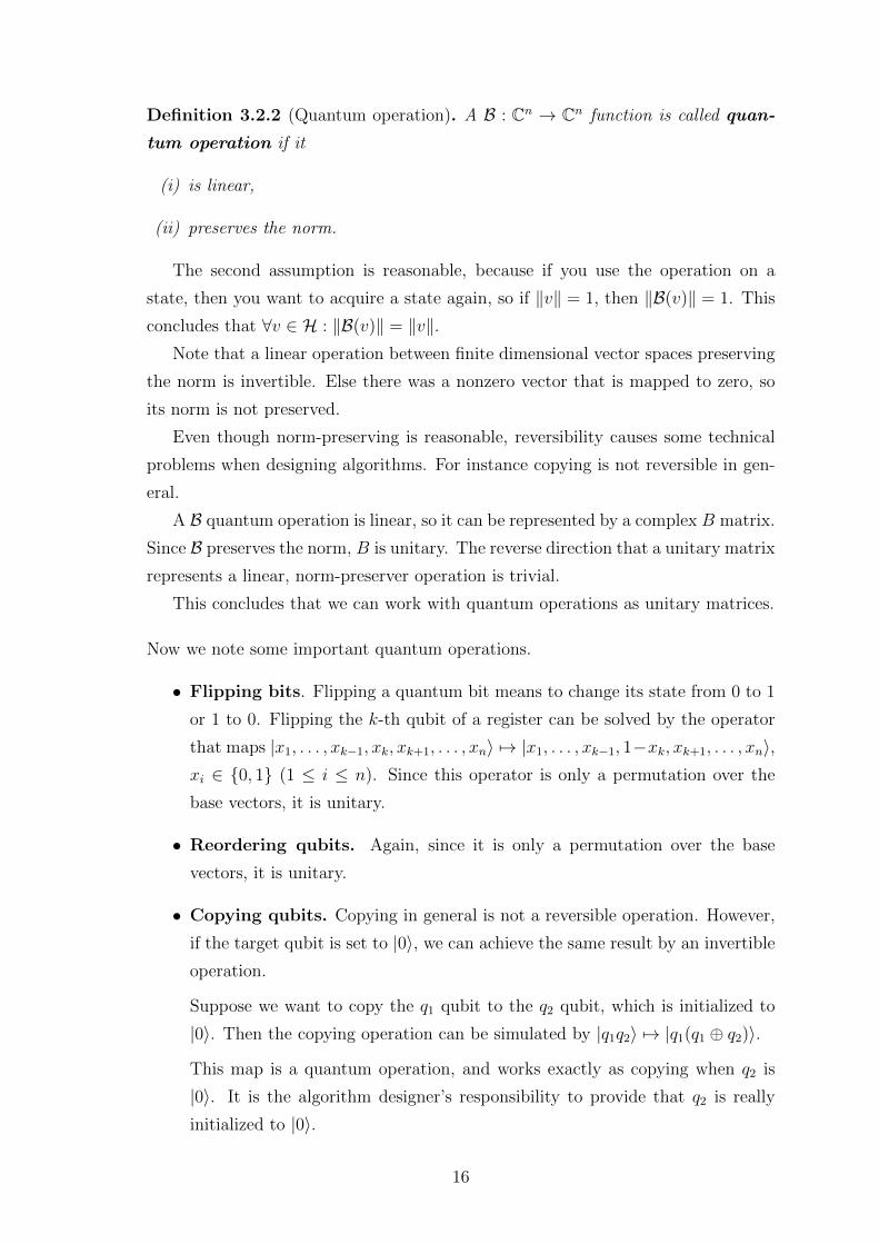
It is often useful to imagine a qubit as a 1 long vector on the 2-dimensional plane.

14

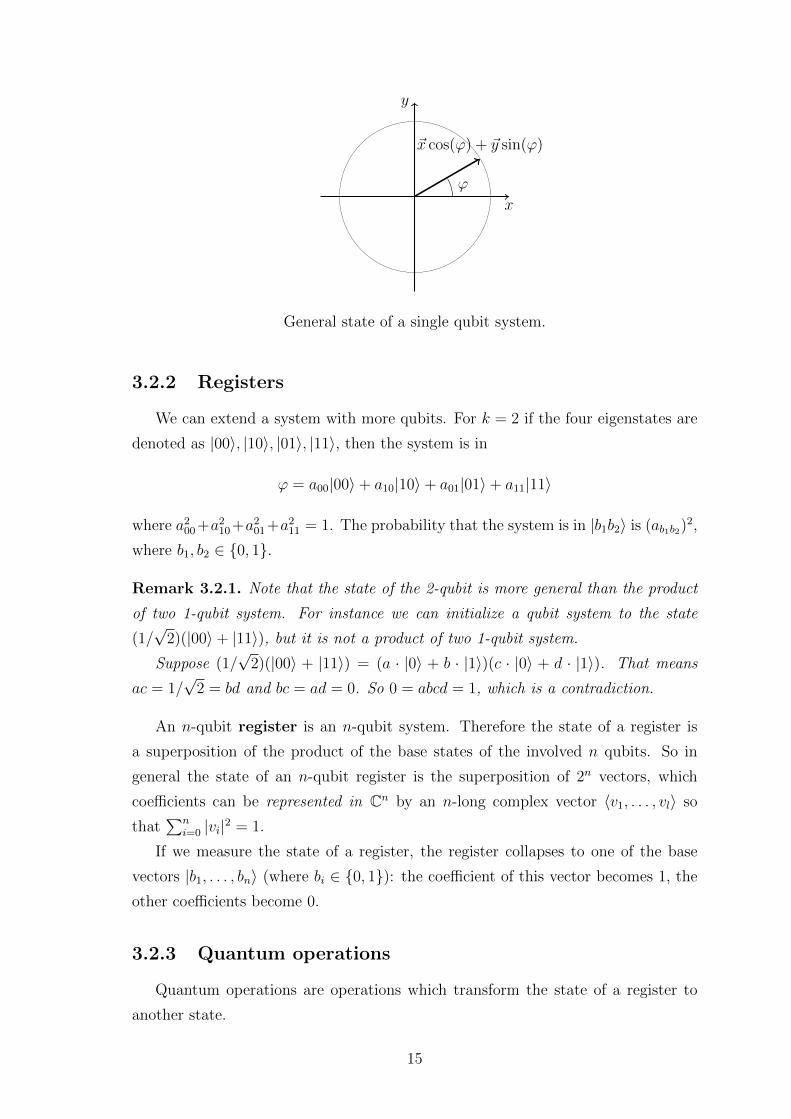
x

y

~x cos(ϕ) + ~y sin(ϕ)

ϕ

General state of a single qubit system.

3.2.2 Registers

We can extend a system with more qubits. For k = 2 if the four eigenstates are

denoted as |00〉, |10〉, |01〉, |11〉, then the system is in

ϕ = a00|00〉+ a10|10〉+ a01|01〉+ a11|11〉

where a200+a210+a201+a211 = 1. The probability that the system is in |b1b2〉 is (ab1b2)2,

where b1, b2 ∈ 0, 1.

Remark 3.2.1. Note that the state of the 2-qubit is more general than the product

of two 1-qubit system. For instance we can initialize a qubit system to the state

(1/√

2)(|00〉+ |11〉), but it is not a product of two 1-qubit system.

Suppose (1/√

2)(|00〉 + |11〉) = (a · |0〉 + b · |1〉)(c · |0〉 + d · |1〉). That means

ac = 1/√

2 = bd and bc = ad = 0. So 0 = abcd = 1, which is a contradiction.

An n-qubit register is an n-qubit system. Therefore the state of a register is

a superposition of the product of the base states of the involved n qubits. So in

general the state of an n-qubit register is the superposition of 2n vectors, which

coefficients can be represented in Cn by an n-long complex vector 〈v1, . . . , vl〉 so

that∑n

i=0 |vi|2 = 1.

If we measure the state of a register, the register collapses to one of the base

vectors |b1, . . . , bn〉 (where bi ∈ 0, 1): the coefficient of this vector becomes 1, the

other coefficients become 0.

3.2.3 Quantum operations

Quantum operations are operations which transform the state of a register to

another state.

15

Definition 3.2.2 (Quantum operation). A B : Cn → Cn function is called quan-

tum operation if it

(i) is linear,

(ii) preserves the norm.

The second assumption is reasonable, because if you use the operation on a

state, then you want to acquire a state again, so if ‖v‖ = 1, then ‖B(v)‖ = 1. This

concludes that ∀v ∈ H : ‖B(v)‖ = ‖v‖.Note that a linear operation between finite dimensional vector spaces preserving

the norm is invertible. Else there was a nonzero vector that is mapped to zero, so

its norm is not preserved.

Even though norm-preserving is reasonable, reversibility causes some technical

problems when designing algorithms. For instance copying is not reversible in gen-

eral.

A B quantum operation is linear, so it can be represented by a complex B matrix.

Since B preserves the norm, B is unitary. The reverse direction that a unitary matrix

represents a linear, norm-preserver operation is trivial.

This concludes that we can work with quantum operations as unitary matrices.

Now we note some important quantum operations.

• Flipping bits. Flipping a quantum bit means to change its state from 0 to 1

or 1 to 0. Flipping the k-th qubit of a register can be solved by the operator

that maps |x1, . . . , xk−1, xk, xk+1, . . . , xn〉 7→ |x1, . . . , xk−1, 1−xk, xk+1, . . . , xn〉,xi ∈ 0, 1 (1 ≤ i ≤ n). Since this operator is only a permutation over the

base vectors, it is unitary.

• Reordering qubits. Again, since it is only a permutation over the base

vectors, it is unitary.

• Copying qubits. Copying in general is not a reversible operation. However,

if the target qubit is set to |0〉, we can achieve the same result by an invertible

operation.

Suppose we want to copy the q1 qubit to the q2 qubit, which is initialized to

|0〉. Then the copying operation can be simulated by |q1q2〉 7→ |q1(q1 ⊕ q2)〉.

This map is a quantum operation, and works exactly as copying when q2 is

|0〉. It is the algorithm designer’s responsibility to provide that q2 is really

initialized to |0〉.

16

• CNOT: Controlled not. The operation defined above above negates the

second qubit if and only if the first qubit is true. This feature also can be

useful in quantum algorithms.

• Rotating a qubit. Since the rotation around the origo in the 2 dimensional

plane is unitary, rotating a qubit is a quantum operation.

• AND. The AND operation is not invertible generally, similarly to the copy

operation. However the same technique can be used when copying.

The AND operation acts on three qubits: the q1, q2 input qubits and a target

qubit q3, which is initialized to |0〉. The AND operation can be expressed as

follows:

|b1〉|b2〉|b3〉 7→ |b1〉|b2〉|b3 ⊕ (b1 ∧ b2)〉.

This operation is unitary, since it is a permutation operation.

• Hadamard operation. The Hadamard operation maps

|b〉 7→ 1√2|0〉+

(−1)b√2|1〉, b ∈ 0, 1.

Its matrix (1 1

1 -1

)is unitary. The Hadamard operation is useful when simulating random algo-

rithms. A single qubit of |0〉 or |1〉 is transformed so that it is a quantum coin:

1/2 : |0〉, 1/2 : |1〉.

Note that if you apply the Hadamard operation to every qubit of an n-qubit

register initialized to |00 . . . 0〉 changes its state to the uniform distribution of

the base states.

Definition 3.2.3 (Elementary quantum operation). A quantum operation is called

elementary if it acts on three or less qubits of a quantum register.

The concept is introduced because in theory it is easy to generate unitary ope-

rations, but in practice it might be difficult to build them. We more possibly build

a quantum operation that works with a few bits.

Definition 3.2.4 (Quantum computation). A series of elementary operations ap-

plied to a quantum register is called quantum computation.

17

3.2.4 The parity game

The parity game is a quantum experiment of John Bell to show the reality of a

contemporary paradox, the Einstein-Podolsky-Rosen Paradox (EPR paradox). Here

we are more interested in the game itself than in the paradox because it is an easy

example when quantum computation is stronger than the classical one.

The parity game works as follows:

There are three players in the game, Alice, Bob and Carol, where Alice and Bob

are in the same team. The game is set up so that Alice and Bob cannot communicate

with each other except from an inital state, when they can agree on a strategy. Carol

can communicate with both Alice and Bob.

First Carol to choose two random bits uniformly noted as x, y ∈R 0, 1. Then

she sends x to Alice and y to Bob. After having received the bits, Alice and Bob to

choose an own bit a and b respectively, and respond it to Carol.

Alice and Bob win if and only if a⊕ b = x ∧ y, or in details:

• if x = 0 or y = 0, then Alice and Bob win if and only if they send back the

same bits, i.e a = b.

• if x = 1 and y = 1, then Alice and Bob win if and only if they send back

different bits, i.e a 6= b.

Theorem 3.2.5. In the classical computational model the maximum winning prob-

ability Alice and Bob can reach is 0.75.

Proof. There are four deterministic strategies from which Alice and Bob can choose:

f : 0, 1 → 0, 1. We will show that these deterministic strategies lead to 0.75

winning probability at most. Therefore any mixed strategy leads to 0.75 probability

at most.

Suppose the strategy of Alice is constant 1. Then if y = 0, Bob should choose

1. If y = 1, then he has to answer with x, which is ∈R 0, 1. So the maximum

probability to win is 12· 1 + 1

2· 12

= 34. The same probability comes out when Alice’s

strategy is constant 0.

This also proves that they can reach 0.75.

Suppose the strategy of Alice is always to send back x, i.e a = x. We have to find

the best strategy for Bob.

• Case y = 1. If Bob chooses 0, they surely win:

– if x = 0, then they should choose the same bits, and a = x = 0 = b.

18

– if x = 1, then they should choose different, and a = x = 1 6= 0 = b.

• Case y = 0. Now they should answer with different bits. If x = 0, he should

choose b = 1, if x = 1 he should choose b = 0. So they can win only with 1/2

at maximum in this subcase.

The total probability for this strategy is therefore 0.75.

The same probability comes out when Alice sends back 1− x.

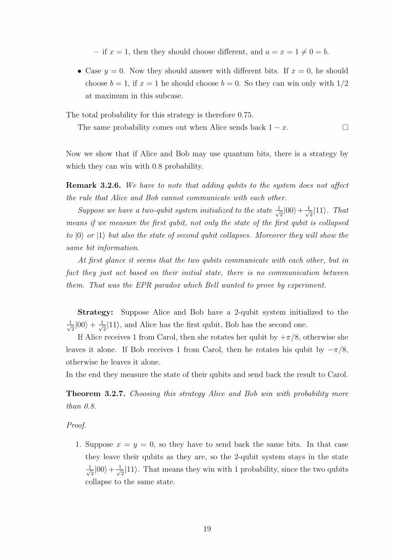
Now we show that if Alice and Bob may use quantum bits, there is a strategy by

which they can win with 0.8 probability.

Remark 3.2.6. We have to note that adding qubits to the system does not affect

the rule that Alice and Bob cannot communicate with each other.

Suppose we have a two-qubit system initialized to the state 1√2|00〉+ 1√

2|11〉. That

means if we measure the first qubit, not only the state of the first qubit is collapsed

to |0〉 or |1〉 but also the state of second qubit collapses. Moreover they will show the

same bit information.

At first glance it seems that the two qubits communicate with each other, but in

fact they just act based on their initial state, there is no communication between

them. That was the EPR paradox which Bell wanted to prove by experiment.

Strategy: Suppose Alice and Bob have a 2-qubit system initialized to the1√2|00〉+ 1√

2|11〉, and Alice has the first qubit, Bob has the second one.

If Alice receives 1 from Carol, then she rotates her qubit by +π/8, otherwise she

leaves it alone. If Bob receives 1 from Carol, then he rotates his qubit by −π/8,

otherwise he leaves it alone.

In the end they measure the state of their qubits and send back the result to Carol.

Theorem 3.2.7. Choosing this strategy Alice and Bob win with probability more

than 0.8.

Proof.

1. Suppose x = y = 0, so they have to send back the same bits. In that case

they leave their qubits as they are, so the 2-qubit system stays in the state1√2|00〉+ 1√

2|11〉. That means they win with 1 probability, since the two qubits

collapse to the same state.

19

2. Suppose x = 0, y = 1. Again, they have to send back the same bits. According

to the strategy, Alice leaves her qubit as it is. With 12

probability she gets 0

when the system collapses to |00〉, so Bob’s qubit collapses to state |0〉. Then

it is rotated by −π/8. In that case their winning probability is cos2(−π/8).

With 12

probability Alice gets 1. Then the system collapses to |11〉, so Bob’s

qubit is set to |1〉, then rotated by −π/8. To win, Bob needs to send back

1. Its probability is sin2(π/2 − π/8) = cos2(π/8). So the total probability is

cos2(π/8) > 0.85.

x

y

~x cos(−π/8) + ~y sin(−π/8)

π/8

When a = 0.

x

y~x cos(π/4− π/8) + ~y sin(π/4− π/8)

π8

When a = 1.

3. Case x = 1, y = 0 is similar to the case above.

4. Case x = 1, y = 1. Now both players rotate their qubits, so we calculate the

state of the 2-qubit system after the rotations.

The calculation is done by simply calculating the rotated state of the eigen-

states |00〉 =(1·|0〉+0·|1〉

)(1·|0〉+0·|1〉

)and |11〉 =

(0·|0〉+1·|1〉

)(0·|0〉+1·|1〉

),

then take the superposition of the result:

1√2·

rot(|00〉)︷ ︸︸ ︷(cos(π/8) · |0〉+ sin(π/8) · |1〉

)·(

cos(π/8) · |0〉 − sin(π/8) · |1〉)

+

1√2

rot(|11〉)︷ ︸︸ ︷(− sin(π/8) · |0〉+ cos(π/8) · |1〉

)·(

sin(π/8) · |0〉+ cos(π/8) · |1〉)

=

1√2·(

cos2(π/8)− sin2(π/8))· |00〉 − 1√

2· 2 sin(π/8) cos(π/8) · |01〉 +

1√2· 2 sin(π/8) cos(π/8) · |10〉+

1√2·(

cos2(π/8)− sin2(π/8))· |11〉

Since cos2(π/8) − sin2(π/8) = cos(π/4) = sin(π/4) = 2 sin(π/8) cos(π/8), the

system can be in the states |00〉, |01〉, |10〉, |11〉 each with probability 1/4. That

means Alice and Bob win with 12

probability.

20

Now we can calculate the total winning probability:

1

4· 1 +

1

4· 0.85 +

1

4· 0.85 +

1

4· 1

2= 0.8

3.3 Quantum computational complexity

3.3.1 Running time

In this section we talk about running time and the complexity class of the poly-

nomial quantum algorithms (BQP). Then we examine how is BQP related to P and

BPP.

Suppose we want to compute an f : 0, 1∗ → 0, 1 in T (n) time, where 0, 1∗

means the finite words over 0, 1.The function f should map from 0, 1∗, since a function can operate on any

long numbers in general. However, a given quantum computation works with a fixed

register, therefore works with fixed number of bits. That means we have to build

quantum computations for every input size. The number of elementary quantum

operations of these quantum computations should be T (n) at maximum as we want

an algorithm running in T (n).

Therefore we have to design T (n)-long quantum computations for every n ∈ N, so

there should be a Turing machine A that prints out the description of the elementary

quantum operations of the quantum computations for n ∈ N. Of course A needs to

be polynomial to make sense.

Finally, since the whole quantum computation is probabilistic, we only demand

the printed quantum computations to realize the function f with probability at least

2/3.

The description of an elementary operation is its complex matrix. However a

complex matrix cannot be presented by finite words, so we write out only the most

significant O(log T (n)) bits of the complex numbers.

Putting this together ([AB09]):

Definition 3.3.1 (Running time). Let f : 0, 1∗ → 0, 1, and T : N → N be

some functions. We say that f is computable in quantum T (n) time if there is a

polynomial time classical Turing Machine that on input (1n, 1T (n)) for any n ∈ Noutputs the descriptions of quantum gates F1, . . . , FT , such that for every x ∈ 0, 1n

we can compute f(x) by the following process with probability at least 23:

21

1. Initialize an m qubit quantum register to the state |x0n−m〉, i.e x is padded with

zeros, where m ≤ T (n).

2. Apply one after the other T (n) elementary quantum operations F1, . . . , FT to

the register.

3. Measure the register and let Y denote the obtained value.

4. Return Y1, i.e the value of the first qubit of the register.

Definition 3.3.2. A Boolean function f : 0, 1∗ → 0, 1 is in BQP if there is a

polynomial p : N→ N, such that f is computable in quantum p(n) time.

3.3.2 P, BPP, BQP

Theorem 3.3.3. If f : 0, 1n → 0, 1m is computable by a classical boolean circuit

of size S, builded from AND, OR, and NOT gates, where the in-degrees of the nodes

are at most 3, then there is a sequence of 2S+m+n quantum operations computing

the mapping

|x〉|02m+s〉 7→ |x〉|0m〉|f(x)〉|0S〉.

Since every classical boolean circuit can be reconstructed so that the in-degrees

are at most 3 by only polynomially increasing the number of gates, the in-degree

restriction is only technical. As a corollary we can simulate boolean circuits by

quantum computations in polynomial time. Since every Turing machine running

in T (n) time has an equivalent Boolean circuit of size O(T (n) log T (n)), we have

P ⊂ BQP .

Proof. In the register we use n bits for the input, m bits for the output, m bits for

saving purposes, and the last S qubits as a scratchpad of the quantum operations.

The scratchpad of a quantum operation is the qubit where the quantum operation

writes its result.

Replace the S gates with their quantum equivalent noted in the previous section.

Note that the AND and OR gates do not change their input. The NOT gate can

be realized by first copying to the scratchpad than flipping the scratchpad bit, so it

does not change its input either. It means that more quantum operations can read

the same input.

Now we apply these quantum operations to the register. Then the register is

mapped to:

|x〉|02m+s〉 7→ |x〉|f(x)〉|0m〉|z〉,

22

where z denotes the value of the value of the scratchpad in the end.

Now using the COPY operation, copy f(x) to 0m:

|x〉|f(x)〉|0m〉|z〉 7→ |x〉|f(x)〉|f(x〉|z〉.

Now apply the inverse of the S quantum gates in reverse order. As a result:

|x〉|f(x)〉|f(x〉|z〉 7→ |x〉|0m〉|f(x〉|0S〉,

which gives the desired result.

Corollary 3.3.4. P ⊂ BQP

Using the Hadamard operation we can simulate random bits: |0〉 is mapped to1√2|0〉+ 1√

2|1〉, so with 1

2− 1

2probability we read |0〉 or |1〉. As a consequence:

Corollary 3.3.5. BPP ⊂ BQP

3.4 Grover’s search algorithm

Grover’s search algorithm is a quantum algorithm for finding a satisfying evalu-

ation of a function ϕ(x) given by a boolean circuit, when the solution of the formula

is unique.

The general case, when ϕ(x) may have more than one solution can be reduced

to this case. In [VV86] Leslie Valiant and Vijay Vazirani showed that given a ϕ

boolean circuit formula, there is a randomized algorithm that with Ω(1/n) proba-

bility transforms ϕ to a ϕ′ formula with a unique solution so that it also satisfies ϕ.

The general version of the problem is called the search problem.

The idea behind the search algorithm is to think of the evaluations as a su-

perposition of n qubits. First we initialize the quantum register to the uniform

distribution of the evaluations. One of these evaluations evaluate f(x) to true, let

it be y0. In each step the the actual evaluation is rotated towards y0. We repeat the

process till we get close enough to y0 so that when reading the register its value is

y0 with high probability.

Grover’s search algorithm

Suppose n ≥ 3. For n = 1, 2 we can try the two or four evaluations. Let ϕ(x)

denote a boolean circuit formula with y0 unique solution. Let

u =1

2n/2

∑x∈0,1n

|x〉

23

denote the uniform state of the quantum register (see Hadamard operation). Since

〈u, y0〉 = 12n/2 , the angle between u and y0 is less than π/2. Let

e =1√

2n − 1

∑x 6=y0,x∈0,1n

|x〉.

Note that e is on the plane spanned by u and y0, and it is orthogonal to y0.

The algorithm starts with w = u. Then in each step it rotates w toward |y0〉 till

the coefficient of y0 in w is greater than 1/√

2, when the measurement collapses w

to y0 with 1/2 probability.

The rotation is solved by two reflections. First we reflect w around e, resulting

in w′. Then we reflect w′ around u. After the two reflection w gets closer to |y0〉 by

2γ, where γ is the angle between u and e.

e

y0

u

w

w′

w′′

2γ

γ

Vector w after the two reflections.

Now we show how the reflections can be done by quantum computations.

Reflecting around e.

First we note the formula of the reflection. Suppose we want to reflect the vector

~p to vector ~q. The vector ~p can be uniquely written as ~p = α~q + ~q⊥, where ~q⊥ is

orthogonal to ~q. Then the reflected vector is ~p = α~q − ~q⊥.

Using this formula the reflection of w around e is∑x 6=y0

wx|x〉 − wy0|y0〉.

We will calculate the reflection in three steps.

(i) In the first transformation we setup an indicator quantum bit that marks the

satisfying evaluation. The transformation uses the boolean circuit ϕ itself,

which is correct since ϕ is polynomial. Technically we should introduce a

24

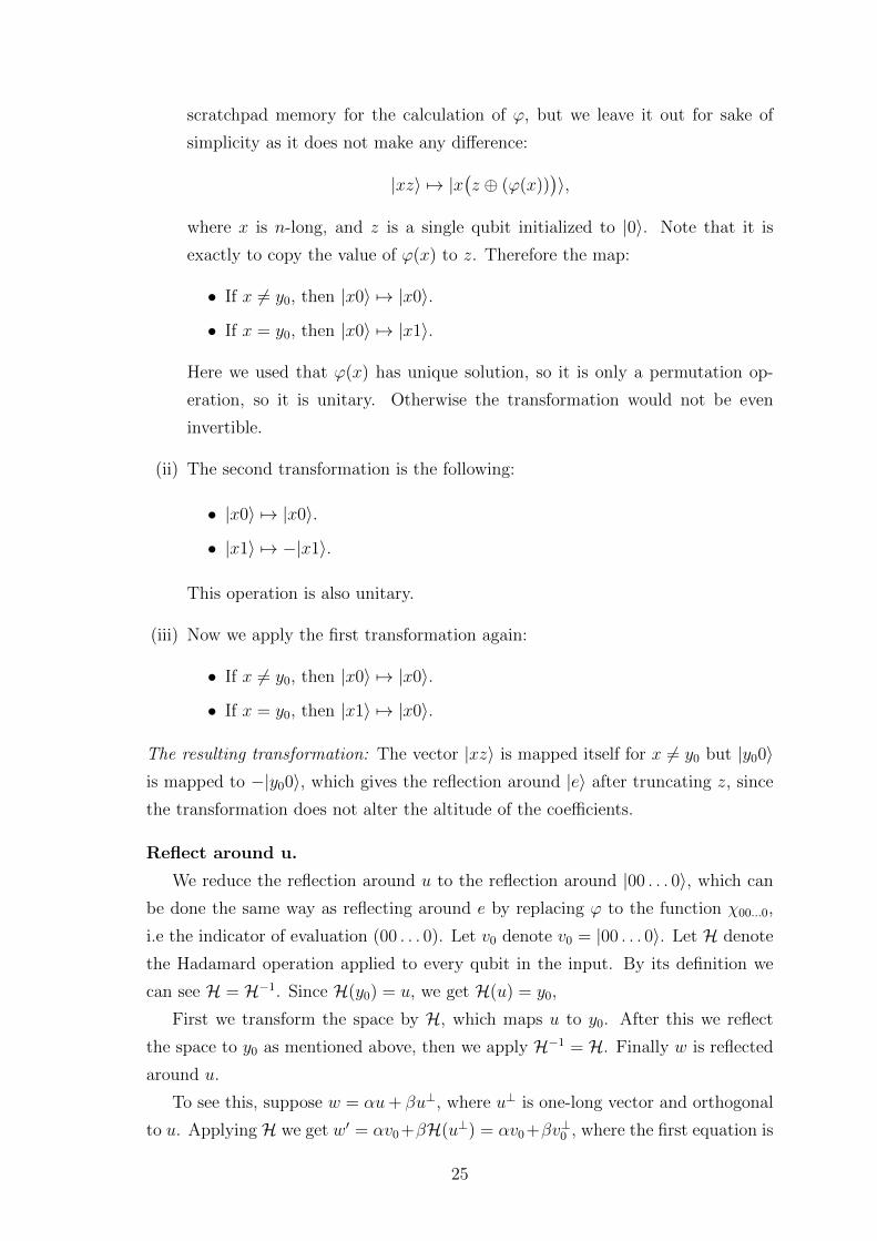
scratchpad memory for the calculation of ϕ, but we leave it out for sake of

simplicity as it does not make any difference:

|xz〉 7→ |x(z ⊕ (ϕ(x))

)〉,

where x is n-long, and z is a single qubit initialized to |0〉. Note that it is

exactly to copy the value of ϕ(x) to z. Therefore the map:

• If x 6= y0, then |x0〉 7→ |x0〉.

• If x = y0, then |x0〉 7→ |x1〉.

Here we used that ϕ(x) has unique solution, so it is only a permutation op-

eration, so it is unitary. Otherwise the transformation would not be even

invertible.

(ii) The second transformation is the following:

• |x0〉 7→ |x0〉.

• |x1〉 7→ −|x1〉.

This operation is also unitary.

(iii) Now we apply the first transformation again:

• If x 6= y0, then |x0〉 7→ |x0〉.

• If x = y0, then |x1〉 7→ |x0〉.

The resulting transformation: The vector |xz〉 is mapped itself for x 6= y0 but |y00〉is mapped to −|y00〉, which gives the reflection around |e〉 after truncating z, since

the transformation does not alter the altitude of the coefficients.

Reflect around u.

We reduce the reflection around u to the reflection around |00 . . . 0〉, which can

be done the same way as reflecting around e by replacing ϕ to the function χ00...0,

i.e the indicator of evaluation (00 . . . 0). Let v0 denote v0 = |00 . . . 0〉. Let H denote

the Hadamard operation applied to every qubit in the input. By its definition we

can see H = H−1. Since H(y0) = u, we get H(u) = y0,

First we transform the space by H, which maps u to y0. After this we reflect

the space to y0 as mentioned above, then we apply H−1 = H. Finally w is reflected

around u.

To see this, suppose w = αu+ βu⊥, where u⊥ is one-long vector and orthogonal

to u. Applying H we get w′ = αv0+βH(u⊥) = αv0+βv⊥0 , where the first equation is

25

true because of the linearity, the second because of the angle-preservation (unitary).

Applying T we get w′′ = αv0 − βv⊥0 , then applying H−1 we get w′′′ = αv0 − βv⊥0 ,

which is exactly the rotated vector of w around u.

In summary, we can solve the reflection around u by applying H to w, then

reflect to |00 . . . 0〉, then apply again H.

Iteration number.

These reflections rotate the vector w 2γ closer to |y0〉. So in O(1/γ) steps we

get nearer to |y0〉 than 2γ. Now we estimate the value of γ.

Note that e, y0, u are in the same plane. The angle between u and y0 is less than

π/2, y0⊥e, and the angle between u and e is γ ≤ π2, meaning the angle between u

and y0 is π/2− γ. Therefore

1

2n/2= 〈u, y0〉 = cos

(π2− γ)

= sin(γ).

We know that for 0 ≤ x ≤ π/2 : (2/π) · x ≤ sin(x) ≤ x. Putting γ into this we get

γ ≥ 1/(2n/2) and γ ≤ π/(2 · 2n/2)That means after the O(1/γ) = O(2n/2) iterations the angle between y0 and w is

less than 2· π2·2n/2 , so the probability to collapse to y0 is cos2

(2 · π

2·2n/2

)≥ cos2(π/4) =

1/2. This gives the desired result.

3.5 Quantum resistance

Grover’s algorithm solves the search problem in O(2n/2) running time. Now we

discuss a result which shows that this is the best possible in a certain sense.

Definition 3.5.1. We call an F : A 7→ B subroutine as a random oracle, if in

one step for any input from A outputs an element of B uniformly in a consistent

way: for a given a ∈ A, F outputs always the same b = F(a) whenever we invoke

F . So a random oracle can be imagined as a machine that for an unasked input

chooses an output randomly, however stores the value, so later instead of generating

again it outputs the stored value.

The computational model where we can invoke a random oracle is called the

random oracle model. The model without the hyphotesis of the existence of a

random oracle is called the standard model. The following result in [BBBV97]

shows that the asymptotics of the Grover’s search algorithm is the best possible in

the random oracle model.

26

Theorem 3.5.2. For every T (n) ∈ o(2n/2), relative to a random oracle chosen

uniformly from the random oracles, with 1 probability, every NP problem cannot be

solved in quantum-T (n) time.

The introduction of a random oracle to a computational model imports such

“blackbox” functions that have no special properties because of the high-level ran-

domness. These functions are get known only by evaluations. So in the random

oracle model we can generate such formulae that cannot be solved by its specific

properties.

In this sense the theorem above states that the quantum search algorithms which

are purely based on the blackbox property of the formulae, cannot solve the search

problem in o(2n/2). It means that the search problem remains resistant in the

quantum computational model.

This does not mean that we are sure there is no polynomial algorithm that solves

the search problem, since the random oracle hypothesis is a strong tool.

Remark 3.5.3. Note that the formula of the satisfiability problem (SAT) is also a

boolean circuit formula. Therefore we believe that we cannot exponentially speedup

the SAT problem only by quantum computers. This means the cryptographic schemes

which security depends on NPC problems remain resistant.

Remark 3.5.4. Another consequence, since many hash functions we use can be

imagined as boolean circuits, they cannot be reverted only by quantum computers.

Therefore the cryptographic schemes which security purely depends on the pre-

image property of the hash function believed to remain resistant.

27

Chapter 4

Resistant digital signatures

Digital signature schemes have a wide range of application areas. Browsers use

them to verify the authenticity of web services, Intrusion Detection Systems (IDS)

to check if a hacker changed system files, archiving and synchronizing algorithms to

minimalize the amount of transmitted data or to verify their integrity, etc.

Since we use digital signature schemes in many situations, it is important that

these schemes to be resistant to quantum computers in order to prevent potential

corruption or forgery. In this thesis we will talk about signature schemes that are

based on the Lamport signature scheme.

4.1 Lamport signature

Lamport signature scheme [Lam79],[Vil11] is a digital signature scheme. Since

its reliability depends only on the properties of the hash function, it is believed to

be resistant to quantum computers, as we mentioned in Remark 3.5.4.

The Lamport signature scheme is the following: Let f be a one-way function.

Let n denote the length of the message digest n.

First we choose 2n random numbers (below a large p prime), these series will be

the private keys.

S0 =(S01 , S

02 , . . . , S

0n

), S1 =

(S11 , S

12 , . . . , S

1n

)The public key will be the hash of the two lists:

f(S01), f(S0

2), . . . , f(S0n), f(S0

1), f(S12), . . . , f(S1

n)

The signature K will be n-long, defined by the following: 0 ≤ i < n,

Ki =

S0i : Mi = 0

S1i : Mi = 1

28

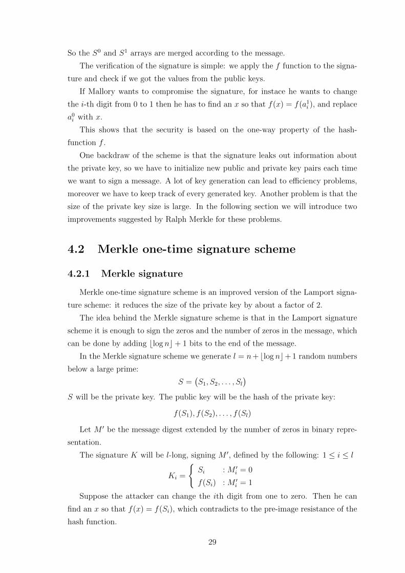
So the S0 and S1 arrays are merged according to the message.

The verification of the signature is simple: we apply the f function to the signa-

ture and check if we got the values from the public keys.

If Mallory wants to compromise the signature, for instace he wants to change

the i-th digit from 0 to 1 then he has to find an x so that f(x) = f(a1i ), and replace

a0i with x.

This shows that the security is based on the one-way property of the hash-

function f .

One backdraw of the scheme is that the signature leaks out information about

the private key, so we have to initialize new public and private key pairs each time

we want to sign a message. A lot of key generation can lead to efficiency problems,

moreover we have to keep track of every generated key. Another problem is that the

size of the private key size is large. In the following section we will introduce two

improvements suggested by Ralph Merkle for these problems.

4.2 Merkle one-time signature scheme

4.2.1 Merkle signature

Merkle one-time signature scheme is an improved version of the Lamport signa-

ture scheme: it reduces the size of the private key by about a factor of 2.

The idea behind the Merkle signature scheme is that in the Lamport signature

scheme it is enough to sign the zeros and the number of zeros in the message, which

can be done by adding blog nc+ 1 bits to the end of the message.

In the Merkle signature scheme we generate l = n+ blog nc+ 1 random numbers

below a large prime:

S =(S1, S2, . . . , Sl

)S will be the private key. The public key will be the hash of the private key:

f(S1), f(S2), . . . , f(Sl)

Let M ′ be the message digest extended by the number of zeros in binary repre-

sentation.

The signature K will be l-long, signing M ′, defined by the following: 1 ≤ i ≤ l

Ki =

Si : M ′

i = 0

f(Si) : M ′i = 1

Suppose the attacker can change the ith digit from one to zero. Then he can

find an x so that f(x) = f(Si), which contradicts to the pre-image resistance of the

hash function.

29

Suppose the attacker wants to change the ith digit from zero to one in the mes-

sage, then he will contradict to the checksum of the number of zeros. Since changing

some zeros to one in the counter only increases its value, he cannot withdraw zeros

from the message.

As a consequence the security of the Merkle signature scheme depends only on

the pre-image resistance of the hash function.

Since the size of the private key has decreased from 2n to n + blog nc + 1, the

size of the private key is reduced by about a factor of two.

4.2.2 Merkle-Winternitz signature scheme

The size of the private keys can be further reduced in trade of performance by

generalizing the technique above.

Above we signed every bits, which can be imagined as signing 1-long blocks.

Instead of signing 1-long blocks we can sign k-long blocks by generating private

random numbers for the block-value 00 . . . 0︸ ︷︷ ︸k

in each block. The signature of a

block-value Bi will be fBi(Si), where fm = f f · · · f︸ ︷︷ ︸m

. The public key will be

f 2k−1(Si).

The verification process is again applying the f function to the blocks till we

receive the public key, and checking if we receive the public key after the right

iteration.

Here again an attacker cannot decrease the value of a block because of the pre-

image resistance of the hash function. However there is a possibility again to increase

the value of a block, so we have to add a checksum to the end of the message, similarly

to the Merkle signature scheme:∑l

i=1(2k− 1−Bi), where l is the number of blocks

and the value of the ith block is Bi. We have to sign the checksum along with the

message.

Since the time of signature and verification increases exponentially by k but the

size of the private key is reduced approximately linearly, the optimal value of k

depending on the hash function is small, usually 2,3,4.

4.2.3 Merke hash tree

Another problem with both Lamport and Merkle signature scheme that we have

to use different public keys for different signatures.

The Merkle hash tree is a verification technique in order to prove that we used

a public key from a given set. So instead of publishing every single public key, we

30

have to publish a proof that we used a legal public key.

If we have generated 2h public private keys in advance, then these keys can be

accumulated into a tree so that finally it is enough to distribute a single key, the

key of the root node.

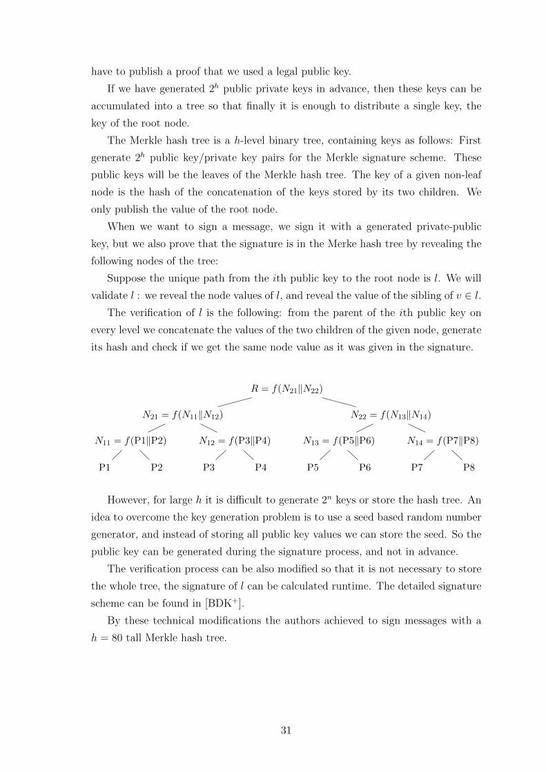
The Merkle hash tree is a h-level binary tree, containing keys as follows: First

generate 2h public key/private key pairs for the Merkle signature scheme. These

public keys will be the leaves of the Merkle hash tree. The key of a given non-leaf

node is the hash of the concatenation of the keys stored by its two children. We

only publish the value of the root node.

When we want to sign a message, we sign it with a generated private-public

key, but we also prove that the signature is in the Merke hash tree by revealing the

following nodes of the tree:

Suppose the unique path from the ith public key to the root node is l. We will

validate l : we reveal the node values of l, and reveal the value of the sibling of v ∈ l.The verification of l is the following: from the parent of the ith public key on

every level we concatenate the values of the two children of the given node, generate

its hash and check if we get the same node value as it was given in the signature.

P1

N11 = f(P1‖P2)

P2

N21 = f(N11‖N12)

P3

N12 = f(P3‖P4)

P4

R = f(N21‖N22)

P5

N13 = f(P5‖P6)

P6

N22 = f(N13‖N14)

P7

N14 = f(P7‖P8)

P8

However, for large h it is difficult to generate 2n keys or store the hash tree. An

idea to overcome the key generation problem is to use a seed based random number

generator, and instead of storing all public key values we can store the seed. So the

public key can be generated during the signature process, and not in advance.

The verification process can be also modified so that it is not necessary to store

the whole tree, the signature of l can be calculated runtime. The detailed signature

scheme can be found in [BDK+].

By these technical modifications the authors achieved to sign messages with a

h = 80 tall Merkle hash tree.

31

Chapter 5

Resistant encryption schemes

5.1 Lattice based encryption

5.1.1 Lattices

There are two equivalent definitions for lattices, a costructive and a structural

definition.

Definition 5.1.1 (Generated lattice). Let b1, . . . , bk ⊂ Rn be linearly independent

vectors. The set L = ∑k

i=1 nibi|n1, . . . , nk ∈ Z is called the lattice generated

by b1, . . . , bk. If B ∈ Rn×k denotes the matrix which columns are bi, then the

generated lattice can be expressed as the following:

L = Bv : v ∈ Zk.

B is called a generator matrix or basis of L.

Definition 5.1.2 (Lattice). A lattice is a discrete, additive subgroup of Rn.

Theorem 5.1.3. L is a generated lattice ⇔ L is a lattice.

Proof. ⇒ A generated lattice is an additive subgroup of Rn, since multiplying by B

is a linear transformation.

To prove that a generated lattice is discrete, we have to show that any bounded

subset of Rn contains only finitely many lattice points.

Let B be a generator matrix of L, and append vectors as columns to B till it

becomes invertible. Denote the new matrix as Q, Q−1 its inverse matrix, and let

α = max|(Q−1)i,j| : 1 ≤ i, j ≤ n. Let L′ denote the lattice generated by Q.

For a z = Qλ ∈ L′ we have λ = Q−1z, therefore |λi| ≤ αn‖z‖. For any bounded

subset of Rn the norm ‖z‖ is bounded, so the integer coefficients of λ is below

32

a dimension-dependent constant. Therefore the bounded subset can only contain

finitely many lattice points from L′, so from L too.

⇐ Suppose L is a discrete subgroup of Rn. Let g1, . . . , gk denote a basis of the

subspace generated by L. Let

X = x ∈ R : x =k∑i=1

λigi, 0 ≤ λi < 1, λi ∈ R.

Since X is bounded, X ∩L is finite. Choose the basis g1, . . . , gk so that their integer

combination Lg is a maximal subset of L: there is no G′ = (g′1, . . . , g′k) so that

Lg $ G′v : v ∈ Zk.

Lemma 5.1.4. X ∩ L = 0.

Proof. By contradiction suppose ∃x∗ 6= 0 : x∗ ∈ X ∩ L. Let

x∗ =k∑i=1

λigi,

where λ is lexicographically minimal. There exists such x∗ since X ∩L is finite. Let

λi be the minimal nonzero coefficient in λ, and denote m the integer 1/λi ≤ m <

1/λi + 1. For this m we have (m− 1)λi < 1 and mλi ≥ 1. Let

z = (mλi − 1)gi +k∑

j=i+1

(mλj − bmλjc)gj ∈ X.

From (m − 1)λi < 1, we have (mλi − 1) < λi, so z <lex λ, which means z = 0. So

the coefficients of z is zero.

Putting this into x∗:

x∗ =1

mgi +

k∑j=i+1

bmλjcm

gj

mx∗ = gi +k∑

j=i+1

(bmλjc)gj

gi = mx∗ −k∑

j=i+1

(bmλjc)gj

Note that we cannot generate x∗ as the integer combination of g1, . . . , gk, since we

can generate it by a non-integer combination, and by the independence of g1, . . . , gk

the generating coefficients are unique.

That means if we substitute gi by x∗, we can generate a strictly larger subset of

L, which is a contradiction.

33

We finish the proof by showing that L is the lattice generated by g1, . . . , gk. Let

v =∑k

i=1 λigi. Since g1, . . . , gk generates the subspace spanned by L, it is enough

to show that v ∈ L. The vector v can be written as

v =k∑i=1

(bλic)gi +k∑i=1

(λi − bλic)gi

X 3k∑i=1

(λi − bλic)gi = v −k∑i=1

(bλic)gi ∈ L.

Therefore∑k

i=1(λi − bλic)gi ∈ X ∩ L = 0. So v =∑k

i=1(bλic)gi is a linear

integer combination of g1, . . . , gk.

If you generate a lattice with two different bases, then the number of basis vectors

in the bases are the same.

Suppose there exist two bases with different sizes. Then the elements of the

larger basis can be expressed as the linear (integer) combination of the elements of

the smaller basis, contradicting the linear independency.

So the dimension of the bases of a lattice is invariant, which leads to

Definition 5.1.5 (Dimension). If B generates the L ⊂ Rn lattice, then the dimen-

sion of L is dimL = |B|. If dimL = n, the L is called full-rank lattice.

From now on we suppose that all lattices are full-rank lattices, so their bases are

represented as invertible square matrices.

If n > 1, then every lattice has infinitely many bases. The following theorem

shows a connection between those bases.

Theorem 5.1.6. B and B′ are bases of the same lattice ⇔ ∃U : B′ = B ·U , where

U is an integer matrix and det(U) = ±1.

Proof.

⇐ Let B be a basis of L, let U be integer matrix with det(U) = ±1. Denote L′

the lattice generated by BU . We have to show that L = L′.Suppose v ∈ L, i.e. ∃λ : Bλ = v. Since the determinant is ±1 of the U integer

matrix, its inverse matrix is also integer. That means the equation Uµ = λ has an

integer solution for µ. Since (BU)µ = B(Uµ) = Bλ = v, v ∈ L′, therefore L ⊆ L′.

Suppose v ∈ L′. That means ∃µ so that BUµ = v. With λ = Uµ, we get

Bλ = v, so L′ ⊆ L.

⇒ Let B and B′ be different bases of L. Since the basis elements are in L, there

exist U,U ′ integer matrices so that B = B′U ′, B′ = BU . Joining the two equations:

34

B(UU ′) = B, therefore 1 = det(UU ′) = det(U) det(U ′). As the determinant of an

integer matrix is integer, det(U) = ±1.

As a corollary, not only the dimension of a lattice is invariant but also the

determinant of the generator matrices.

Corollary 5.1.7. If B and B′ are bases of the same L lattice, then detB = detB′.

The common value of the determinants is noted as vol(L).

Although there are many different bases for the same lattice, it is useful to know

a basis which has nearly orthogonal and short vectors.

One indices of quality of a basis is the weight:

Definition 5.1.8 (Weight). Let B = b1, b2, . . . , bn be a basis of L. Then the

weight of B is:

‖B‖ =n∏i=1

‖bi‖

Note that if the basis vectors are orthogonal, then the weight is equal to the

determinant of the lattice.

If B and B′ are bases of the same L and ‖B‖ > ‖B′‖, then we say B′ is reduced

relative to B.

Since the determinant of the vectors of a parallelepipedon is smaller than the

product of their length, we get that vol(L) is a lower bound to the weight.

Theorem 5.1.9 (Hadamard).

‖B‖ ≥ vol(L),

There is equality if and only if the columns of B are orthogonal.

The following theorem of Minkowski states that there are no arbitrary large gaps

in a lattice. Using this theorem we can give an upper bound to the shortest vector

of a lattice.

Theorem 5.1.10. Let L be a lattice so that dimL = n. Then every compact convex

symmetric region of which volume is at least 2n vol(L) contains a nonzero lattice

point.

Proof. We prove the theorem in two parts, first for sets where vol(A) > 2n vol(L),

then by compactness where vol(A) = 2n vol(L).

Suppose A ⊂ R is a compact, convex, symmetric set so that vol(A) > 2n vol(L).

Let g1, . . . , gn be an arbitrary basis of L, and

X = a1g1 + · · ·+ angn : 0 ≤ ai < 1, 1 ≤ i ≤ n.

35

If we shift A with all lattice vectors, it gives a cover of Rn. Specially A is also

covered, so ∀a ∈ A can be written as a = l + x where l ∈ L, x ∈ X. We show that

this decomposition is unique.

Suppose for x =∑xigi ∈ X, x′ =

∑x′igi ∈ X, l =

∑ligi ∈ L, l′ =

∑l′igi ∈ L

we have l + x = l′ + x′. Since the basis vectors are linearly independent, we have

li + xi = l′i + x′i, meaning xi − x′i is an integer, but −1 < xi − x′i < 1, so xi = x′i.

Therefore x = x′, l = l′. As a result we can define the following function:

g : A→ X, a 7→ x.

Now we shrink A by 2. The volume of (1/2)A = (1/2)a ∈ A is vol((1/2)A) =

(1/2n) vol(A) > vol(L) by our assumption. As vol(L) is the volume of the pa-

rallelepipedon X, vol(L) = vol(X), so we get vol((1/2)A) > vol(X). Therefore

there are two points (a1, a2) in 12A which is mapped by g|(1/2)A to the same point

x ∈ X: ∃l1, l2 ∈ L so that a1 = l1 + x, a2 = l2 + x.

After substraction: 0 6= a1 − a2 = l1 − l2 ∈ L. Since a1, a2 ∈ (1/2)A we have

2a1, 2a2 ∈ A, and by simmetry 2a1,−2a2 ∈ A. Since the mid-point of the segment

(2a1,−2a2) is a1 − a2 and A is convex, we have a1 − a2 ∈ A. That means l1 − l2 is

a lattice point in A, proving the first part of the theorem.

Suppose now vol(A) = 2n vol(L). Then we generate nonzero lk lattice points for

regions (1 + 1/k)A using the first part, since (1 + 1/k)A is also compact, convex

subset of Rn, but its volume is vol((1 + (1/k))X) > 2n vol(L). Since the series

(li)i ⊂ 2A, which is bounded subset of Rn, (li)i consists of only finitely many lattice

points. Since by compactness⋂nk=1 (1 + 1/k)A = A , there must be a nonzero

lattice point in A.

As a corollary of Minkowski theorem we have an upper bound for the shortest

vector of L.

Corollary 5.1.11. If L is a lattice, then there is a v ∈ L so that

‖v‖ ≤ cn vol(L)1n ,

where cn is a dimension-dependent constant.

Proof. Let Rnr = x ∈ Rn : ‖x| ≤ r. It is known that

vol(Rnr ) ∼

(2πe

n

)n/2rn,

therefore exists C1, C2 for every n ∈ N:

C1

(2πe

n

)n/2rn ≤ vol(Rn

r ) ≤ C2

(2πe

n

)n/2rn

36

So choosing r = 1n√C1

√2nπe

vol(L)1/n, we have vol(Rnr ) ≥ 2n vol(L). From Minkowski

theorem there is a nonzero lattice point in Rnr , so the length of the shortest nonzero

vector is less than 1n√C1

√2nπe

vol(L)1/n = cn · vol(L)1/n.

5.1.2 Lattice based encryption

In this section we introduce two encryption schemes which are considered to

be resistant to quantum computers. The first scheme is the Goldreich-Goldwasser-

Halevi (GGH) encryption scheme, which is based on solving the closest vector prob-

lem. The second is the NTRU cryptosystem which works with polynomials, however

it is strongly related to lattices. Its security is based on the shortest vector problem.

Problem 5.1.12 (Closest vector problem, CVP). Given an L lattice and v0 ∈ Rn,

find a v ∈ L so that ‖v − v0‖ is minimal.

Problem 5.1.13 (Shortest vector problem, SVP). Given an L lattice, find a nonzero

v ∈ L so that ‖v‖ is minimal.

It is proven that the SVP is NP-hard, and the CVP is at least as hard as the

SVP. As we mentioned in Remark 3.5.3, an NPC problem is believed to be quantum

resistant. Since NP-hard problems are more difficult than the NPC problems, they

are also believed to be quantum resistant.

Practically if we want to solve the SVP or the CVP, it is useful to find a basis

so that has short and nearly orthogonal vectors. Changing a basis for a better basis

is called lattice reduction.

A well-known lattice reduction algorithm is the Lenstra-Lenstra-Lovasz (LLL)

algorithm. It was the first algorithm that could find good lattice reduction in poly-

nomial time. Although the LLL algorithm finds relatively long basis vectors, it is

good enough to break some lattice based cryptographic systems.

5.1.3 GGH cryptographic scheme

Let L be a lattice. The private key is a basis V = v1, . . . , vn with small and

nearly orthogonal basis vectors, the public key is a basis W = w1, . . . , wn with

long and less orthogonal vectors. The idea behind the scheme is to choose the basis

V so that we can solve the CVP problem with it, but with W we cannot.

Let m be an n-long binary vector, the text we want to cypher. To cypher the m

37

message, we calculate the vector e, which will be the cyphertext:

e = r +n∑i=1

miwi,

where r is a small random perturbation vector.

During decryption we calculate the closest x lattice vector to e. That removes

the noise, so we have

x =n∑i=1

miwi.

Hence we can calculate the coefficients by solving this equation.

To calculate the shortest vector x we will use the private key. First we solve the

equation

e =n∑i=1

yivi,

where yi ∈ R, so the coefficients are real. Rounding the coefficients to the nearest

integer we get

u =n∑i=1

byievi,

which is the closest vector if V is chosen well enough.

For small dimensions the LLL algorithm can reduce W so that it can break

the scheme, for moderate dimensions there are variants for LLL that break the

system. Therefore in order to achieve reasonably high security we have to use so

high dimensional vectors that might be impractical.

The size of the keys in the cryptographic scheme is O(n2).

5.2 Polynomial based encryption

5.2.1 NTRU cryptosystem

The cryptosystem works in the ring R = Zr[X]/(xN − 1), where N is a prime.

This ring is a polynomial ring, where the coefficients are from Zr, with the rule

xN ≡ 1. Therefore any element of this ring can be reduced to a polynomial at most

N − 1 degree.

In R we can solve addition and multiplication, and by the Euclidean algorithm

the inverse calculation.

Key generation Fix an N prime, p < q integers so that gcd(p, q) = 1. Usually q is

chosen as a power of 2, and p very small. Choose random f, g ∈ R polynomials with

38

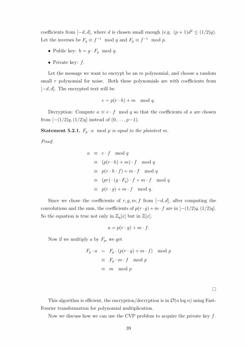
coefficients from [−d, d], where d is chosen small enough (e.g. (p + 1)d2 ≤ (1/2)q).

Let the inverses be Fq ≡ f−1 mod q and Fp ≡ f−1 mod p.

• Public key: h = g · Fq mod q.

• Private key: f .

Let the message we want to encrypt be an m polynomial, and choose a random

small r polynomial for noise. Both these polynomials are with coefficients from

[−d, d]. The encrypted text will be

e = p(r · h) +m mod q.

Decryption: Compute a ≡ e · f mod q so that the coefficients of a are chosen

from [−(1/2)q, (1/2)q] instead of (0, . . . , p−1).

Statement 5.2.1. Fp · a mod p is equal to the plaintext m.

Proof.

a ≡ e · f mod q

≡ (p(r · h) +m) · f mod q

≡ p(r · h · f) +m · f mod q

≡ (pr) · (g · Fq) · f +m · f mod q

≡ p(r · g) +m · f mod q.

Since we chose the coefficients of r, g,m, f from [−d, d], after computing the

convolutions and the sum, the coefficients of p(r · g) +m · f are in [−(1/2)q, (1/2)q].

So the equation is true not only in Zq[x] but in Z[x].

a = p(r · g) +m · f.

Now if we multiply a by Fp, we get

Fp · a = Fp · (p(r · g) +m · f) mod p

≡ Fp ·m · f mod p

≡ m mod p

This algorithm is efficient, the encryption/decryption is in O(n log n) using Fast-

Fourier transformation for polynomial multiplication.

Now we discuss how we can use the CVP problem to acquire the private key f .

39

5.2.2 Connection to lattices

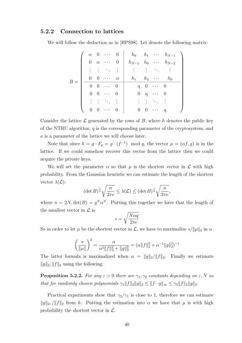
We will follow the deduction as in [HPS98]. Let denote the following matrix:

B =

α 0 · · · 0

0 α · · · 0...

.... . .

...

0 0 · · · α

h0 h1 · · · hN−1

hN−1 h0 · · · hN−2...

.... . .

...

h1 h2 · · · h0

0 0 · · · 0

0 0 · · · 0...

.... . .

...

0 0 · · · 0

q 0 · · · 0

0 q · · · 0...

.... . .

...

0 0 · · · q

Consider the lattice L generated by the rows of B, where h denotes the public key

of the NTRU algorithm, q is the corresponding parameter of the cryptosystem, and

a is a parameter of the lattice we will choose later.

Note that since h = g · Fq = g · (f−1) mod q, the vector µ = (αf, g) is in the

lattice. If we could somehow recover this vector from the lattice then we could

acquire the private keys.

We will set the parameter α so that µ is the shortest vector in L with high

probability. From the Gaussian heuristic we can estimate the length of the shortest

vector λ(L):

(detB)1n

√n

2πe≤ λ(L) ≤ (detB)

1n

√n

2πe,

where n = 2N, det(B) = qNαN . Putting this together we have that the length of

the smallest vector in L is

s =

√Nαq

2πe

So in order to let µ be the shortest vector in L, we have to maximalize s/‖µ‖2 in α.(s

‖µ‖

)2

=α

α2‖f‖22 + ‖g‖22= (α‖f‖22 + α−1‖g‖22)−1

The latter formula is maximalized when α = ‖g‖2/‖f‖2. Finally we estimate

‖g‖2, ‖f‖2 using the following:

Proposition 5.2.2. For any ε > 0 there are γ1, γ2 constants depending on ε,N so

that for randomly chosen polynomials γ1‖f‖2‖g‖2 ≤ ‖f · g‖∞ ≤ γ2‖f‖2‖g‖2.

Practical experiments show that γ2/γ1 is close to 1, therefore we can estimate

‖g‖2, /‖f‖2 from h. Putting the estimation into α we have that µ is with high

probability the shortest vector in L.

40

Bibliography

[AB09] Sanjeev Arora and Boaz Barak. Computational Complexity - A Modern

Approach. Cambridge University Press, 2009.

[BBBV97] Charles H. Bennett, Ethan Bernstein, Gilles Brassard, and Umesh Vazi-

rani. Strengths and weaknesses of quantum computing. SIAM J. Com-

put., 26(5):1510–1523, October 1997.

[BDK+] Johannes Buchmann, Erik Dahmen, Elena Klintsevich, Katsuyuki

Okeya, Camille Vuillaume, and Technische Universitat Darmstadt.

Merkle signatures with virtually unlimited signature capacity.

[HPS98] Jeffrey Hoffstein, Jill Pipher, and Joseph H. Silverman. Ntru: A ring-

based public key cryptosystem. ANTS, pages 267–288, 1998.

[Lam79] Leslie Lamport. Constructing digital signatures from a one way function.

Technical Report CSL-98, SRI International, October 1979.

[LJMP90] Arjen K. Lenstra, Hendrik W. Lenstra Jr., Mark S. Manasse, and

John M. Pollard. The number field sieve. STOC, pages 564–572, 1990.

[Mat03] D. V. Matyukhin. On asymptotic complexity of computing discrete log-

arithms over gf(p). Discrete Mathematics and Applications, 13, 2003.

[O00] Bernhard Omer. Quantum programming in qcl. Master thesis, computing

science, 2000.

[Sho97] Peter W. Shor. Polynomial-time algorithms for prime factorization

and discrete logarithms on a quantum computer. SIAM J. Comput.,

26(5):1484–1509, 1997.

[Vil11] V. I. Villanyi. Signature schemes in single and multi-user settings. Pro-

Quest, UMI Dissertation Publishing, 2011.

[VV86] Leslie G. Valiant and Vijay V. Vazirani. Np is as easy as detecting unique

solutions. Theor. Comput. Sci., 47(3):85–93, 1986.

41

NYILATKOZAT

Név:

ELTE Természettudományi Kar, szak:

ETR azonosító:

Szakdolgozat címe:

A szakdolgozat szerzőjeként fegyelmi felelősségem tudatában kijelentem, hogy a

dolgozatom önálló munkám eredménye, saját szellemi termékem, abban a hivatkozások és

idézések standard szabályait következetesen alkalmaztam, mások által írt részeket a

megfelelő idézés nélkül nem használtam fel.

Budapest, 20 _______________________________

a hallgató aláírása