Masaryk University, Faculty of Informatics

w !"#$%&'()+,-./012345<yA|

Quantum Programming LanguageLanQ

Hynek Mlnarık

PhD Thesis

Brno, Czech Republic September 2007

Acknowledgments

This work would not be realized without support of many people who helped me both proffes-sionally and personally.

I would like to thank my supervisor, Jozef Gruska, for his guidance, support and advicesduring my PhD studies.

I would like also to express my thanks to Lukas Bohac, Jan Bouda, Simon Gay, PhilippeJorrand, Rajagopal Nagarajan, Nick Papanikolaou, Simon Perdrix, Igor Peterlık, Libor Skar-vada, Josef Sprojcar and Tomoyuki Yamakami for their enthusiasm and invaluable commentson LanQ and related discussions. I would like to particularly thank to Rajagopal Nagarajanand Nick Papanikolaou for their hospitality, encouragement and fruitful discussions not onlyduring my visit to the University of Warwick.

Finally, I would like to express my deep gratitude to my wife Lucie and to my parentsfor their endless support and love without which I would never have been able to write thisthesis.

This work was realized under financial support of grants MSM0021622419, GACR201/04/1153 and GACR 201/07/0603.

i

ii

Contents

I Introduction 1

1 Introduction 31.1 The history of quantum information processing . . . . . . . . . . . . . . . . . 31.2 Introduction to quantum computing . . . . . . . . . . . . . . . . . . . . . . . 4

1.2.1 Basics of quantum mechanics . . . . . . . . . . . . . . . . . . . . . . . 41.3 Models of quantum computation . . . . . . . . . . . . . . . . . . . . . . . . . 12

1.3.1 Models based on classical models . . . . . . . . . . . . . . . . . . . . . 121.3.2 Measurement-based computation . . . . . . . . . . . . . . . . . . . . . 13

1.4 Introduction to programming languages . . . . . . . . . . . . . . . . . . . . . 141.4.1 Quantum programming languages . . . . . . . . . . . . . . . . . . . . 16

1.5 Introduction to process algebras . . . . . . . . . . . . . . . . . . . . . . . . . . 171.5.1 Quantum process algebras . . . . . . . . . . . . . . . . . . . . . . . . . 18

2 Current state of the art 192.1 Functional languages and λ-calculi . . . . . . . . . . . . . . . . . . . . . . . . 19

2.1.1 Quantum λq-calculus – van Tonder . . . . . . . . . . . . . . . . . . . . 192.1.2 QPL . . . . . . . . . . . . . . . . . . . . . . . . . . . . . . . . . . . . . 202.1.3 QML . . . . . . . . . . . . . . . . . . . . . . . . . . . . . . . . . . . . . 202.1.4 Quantum λ-calculus – Selinger & Valiron . . . . . . . . . . . . . . . . 212.1.5 nQML . . . . . . . . . . . . . . . . . . . . . . . . . . . . . . . . . . . . 21

2.2 Other languages . . . . . . . . . . . . . . . . . . . . . . . . . . . . . . . . . . 222.2.1 qGCL . . . . . . . . . . . . . . . . . . . . . . . . . . . . . . . . . . . . 222.2.2 QCL . . . . . . . . . . . . . . . . . . . . . . . . . . . . . . . . . . . . . 222.2.3 Q language . . . . . . . . . . . . . . . . . . . . . . . . . . . . . . . . . 232.2.4 QMC . . . . . . . . . . . . . . . . . . . . . . . . . . . . . . . . . . . . 23

2.3 Quantum process algebras . . . . . . . . . . . . . . . . . . . . . . . . . . . . . 242.3.1 CQP . . . . . . . . . . . . . . . . . . . . . . . . . . . . . . . . . . . . . 242.3.2 QPAlg . . . . . . . . . . . . . . . . . . . . . . . . . . . . . . . . . . . . 24

2.4 Summary . . . . . . . . . . . . . . . . . . . . . . . . . . . . . . . . . . . . . . 25

II LanQ programming language 27

3 Introduction 293.1 Informal introduction . . . . . . . . . . . . . . . . . . . . . . . . . . . . . . . 29

iii

CONTENTS

4 Syntax 334.1 Concrete syntax . . . . . . . . . . . . . . . . . . . . . . . . . . . . . . . . . . 334.2 Internal syntax . . . . . . . . . . . . . . . . . . . . . . . . . . . . . . . . . . . 354.3 Configuration syntax . . . . . . . . . . . . . . . . . . . . . . . . . . . . . . . . 36

5 Typing 395.1 Typing rules . . . . . . . . . . . . . . . . . . . . . . . . . . . . . . . . . . . . . 39

6 Basic concepts 456.1 Notation . . . . . . . . . . . . . . . . . . . . . . . . . . . . . . . . . . . . . . . 456.2 Reference-related concepts . . . . . . . . . . . . . . . . . . . . . . . . . . . . . 456.3 Variable-related concepts . . . . . . . . . . . . . . . . . . . . . . . . . . . . . 46

7 Operational semantics 497.1 Memory model . . . . . . . . . . . . . . . . . . . . . . . . . . . . . . . . . . . 497.2 Variable properties storage . . . . . . . . . . . . . . . . . . . . . . . . . . . . 517.3 Configuration . . . . . . . . . . . . . . . . . . . . . . . . . . . . . . . . . . . . 547.4 Variable properties handling functions . . . . . . . . . . . . . . . . . . . . . . 567.5 Local memory handling functions . . . . . . . . . . . . . . . . . . . . . . . . . 587.6 Functions for handling aliasfor constructs . . . . . . . . . . . . . . . . . . . . 607.7 Internal values . . . . . . . . . . . . . . . . . . . . . . . . . . . . . . . . . . . 637.8 Transitions . . . . . . . . . . . . . . . . . . . . . . . . . . . . . . . . . . . . . 637.9 Runtime errors . . . . . . . . . . . . . . . . . . . . . . . . . . . . . . . . . . . 647.10 Processes and configurations . . . . . . . . . . . . . . . . . . . . . . . . . . . . 65

7.10.1 Structural congruence . . . . . . . . . . . . . . . . . . . . . . . . . . . 657.10.2 Nondeterminism and parallelism . . . . . . . . . . . . . . . . . . . . . 66

7.11 Evaluation . . . . . . . . . . . . . . . . . . . . . . . . . . . . . . . . . . . . . . 667.11.1 Basic rules . . . . . . . . . . . . . . . . . . . . . . . . . . . . . . . . . 667.11.2 Promotable expressions . . . . . . . . . . . . . . . . . . . . . . . . . . 677.11.3 Allocation . . . . . . . . . . . . . . . . . . . . . . . . . . . . . . . . . . 677.11.4 Variable declaration . . . . . . . . . . . . . . . . . . . . . . . . . . . . 677.11.5 Assignment . . . . . . . . . . . . . . . . . . . . . . . . . . . . . . . . . 687.11.6 Block . . . . . . . . . . . . . . . . . . . . . . . . . . . . . . . . . . . . 707.11.7 Conditional statement – if . . . . . . . . . . . . . . . . . . . . . . . . . 707.11.8 Conditional cycle – while . . . . . . . . . . . . . . . . . . . . . . . . . 707.11.9 Method call . . . . . . . . . . . . . . . . . . . . . . . . . . . . . . . . . 717.11.10Returning from a method . . . . . . . . . . . . . . . . . . . . . . . . . 727.11.11Forking . . . . . . . . . . . . . . . . . . . . . . . . . . . . . . . . . . . 737.11.12Measurement . . . . . . . . . . . . . . . . . . . . . . . . . . . . . . . . 737.11.13Communication . . . . . . . . . . . . . . . . . . . . . . . . . . . . . . . 75

8 Unique resource ownership 778.1 Unique quantum system ownership . . . . . . . . . . . . . . . . . . . . . . . . 778.2 Unique channel end ownership . . . . . . . . . . . . . . . . . . . . . . . . . . 798.3 Unique channel ownership . . . . . . . . . . . . . . . . . . . . . . . . . . . . . 80

iv

CONTENTS

9 Type soundness 839.1 Typing of configurations . . . . . . . . . . . . . . . . . . . . . . . . . . . . . . 839.2 Progress . . . . . . . . . . . . . . . . . . . . . . . . . . . . . . . . . . . . . . . 849.3 Type preservation . . . . . . . . . . . . . . . . . . . . . . . . . . . . . . . . . 88

9.3.1 Evaluation theorems . . . . . . . . . . . . . . . . . . . . . . . . . . . . 889.3.2 Type preservation lemmata . . . . . . . . . . . . . . . . . . . . . . . . 97

9.4 Type soundness . . . . . . . . . . . . . . . . . . . . . . . . . . . . . . . . . . . 109

10 Comparison with related work 11110.1 LanQ . . . . . . . . . . . . . . . . . . . . . . . . . . . . . . . . . . . . . . . . 11110.2 Omer: QCL . . . . . . . . . . . . . . . . . . . . . . . . . . . . . . . . . . . . . 11110.3 Gay, Nagarajan: CQP . . . . . . . . . . . . . . . . . . . . . . . . . . . . . . . 11410.4 Jorrand, Lalire: QPAlg . . . . . . . . . . . . . . . . . . . . . . . . . . . . . . . 116

11 Conclusion 119

References 121

III Appendix 131

A Program execution example 133

B Implementation 139B.1 LanQ simulator . . . . . . . . . . . . . . . . . . . . . . . . . . . . . . . . . . . 139B.2 Reference manual . . . . . . . . . . . . . . . . . . . . . . . . . . . . . . . . . . 140

B.2.1 Statements . . . . . . . . . . . . . . . . . . . . . . . . . . . . . . . . . 140B.2.2 Quantum operators . . . . . . . . . . . . . . . . . . . . . . . . . . . . 141B.2.3 Variable declarations . . . . . . . . . . . . . . . . . . . . . . . . . . . . 143B.2.4 Expressions . . . . . . . . . . . . . . . . . . . . . . . . . . . . . . . . . 143B.2.5 Operators and methods . . . . . . . . . . . . . . . . . . . . . . . . . . 144

v

CONTENTS

vi

Preface

The original motivation for development of LanQ was the need of an imperative quantumprogramming language with the syntax similar to some well-known classical language, well-defined semantics, and an existing simulator. Moreover, this language was requested tosupport implementation of multiparty protocols.

Such a language can be used by the scientists working in the quantum information process-ing theory field to implement and test their ideas of new quantum algorithms and protocols.They would learn the language easily because it is similar to something they already know.The existing semantics enables them to formally verify various program properties. More-over, the simulator could be connected to existing verification tools thus supporting machine-assisted verification. Further, it could benefit from existing optimization techniques to helpin semi- or fully automatic optimizations of the implemented algorithms and protocols.

In the thesis, we define a typed imperative quantum programming language LanQ thatallows programmers to implement any algorithm that is based on either classical or quantumcomputation or a combination of both. It has well-defined operational semantics, and typesoundness of its part lacking communication capabilities is proved. It allows programmers toassign one quantum system to several variables in such a way that all quantum principles,namely no-cloning and no-deleting, are obeyed. The language syntax is similar to that of Clanguage.

The developed language has several process algebraic features such as creation a newprocess (this is done by forking a new process from a running one) and interprocess com-munication. It therefore supports implementation of multiparty protocols. The quantumresources are proved to be always accessible to at most one process and the channel resourcesto at most two processes at a time. We prove type soundness for unrestricted languageprovided the programs are guaranteed to use only a well-formed communication.

The first part of the thesis offers an introduction to the fields used in the thesis in Chapter 1and provides a list of related work in Chapter 2.

The second part presents the developed quantum programming language LanQ. We for-mally describe the language syntax in Chapter 4, its type system in Chapter 5, definitionsof auxiliary functions and structures in Chapter 6, and its memory model and operationalsemantics in Chapter 7. Further, we prove the unique resource ownership property in Chap-ter 8, and type soundness in Chapter 9. Detailed comparison with several related formalismsis given in Chapter 10.

The appendices form the last part of the thesis. We show an example run of a randomnumber generator implemented in the language in Appendix A, and provide a description ofthe implementation of LanQ simulator in Appendix B. The simulator is publicly available athttp://lanq.sf.net/

vii

Part I

Introduction

1

Chapter 1

Introduction

1.1 The history of quantum information processing

Quantum information processing is a relatively young branch of computer science and physics.It combines paradigms of classical computer science and methods of information processingwith the phenomena exhibited in the quantum world on the basis of the laws of quantummechanics.

The birth of quantum information processing was motivated by several things. It wasFeynman in 1982 who observed that there cannot exist any efficient classical algorithm for sim-ulating quantum mechanics [Feynman, 1982]. It was then suggested that building a computerbased on the quantum mechanical principles could help in this simulation. It was conjecturedthat a quantum computer could use less resources and/or solve several types of problemsfaster than classical computers. Another motivation came from the field of microelectronics.Current design of processors leads to so small sizes that in only a few decades, according toMoore’s law [Moore, 1965], circuit elements would reach atomic level where quantum phe-nomena inevitably appear. Then anyone designing such small circuits would necessarily needto know how to deal with the quantum phenomena. The third big motivation for develop-ment of quantum information processing is a better understanding of the quantum world andcreation of formalisms and tools that help in handling quantum phenomena.

The first contribution to quantum information processing field was published in 1984 byBennett and Brassard – a quantum key distribution protocol known nowadays as BB84 proto-col [Bennett and Brassard, 1984] which is proved to be unconditionally secure [Mayers, 1996].This was the first published work showing the relation of quantum information processing tocryptography. The next contribution to a family of quantum secure key distribution protocolswas given by Ekert in 1991 [Ekert, 1991]. Ekert’s protocol uses quantum entanglement – aspecific correlation of several quantum particles not exhibited in the classical world. Bennett,Brassard and Mermin in 1992 created a simplier scheme for quantum key distribution whichis also based on entanglement [Bennett, Brassard, and Mermin, 1992].

Teleportation of a quantum bit [Bennett, Brassard, Crepeau, Jozsa, Peres, and Woot-ters, 1993] is a protocol which illustrates another feature of the quantum world which is notobserved in the classical world. Classically, when we want to move information from onepart of a system to another, we must send the physical medium containing the data to thedestination. Surprisingly, this is not necessary in the quantum world. Quantum state can beteleported to the destination without physically moving the particle whose state is teleported,

3

1.2. INTRODUCTION TO QUANTUM COMPUTING

only two auxiliary classical bits are needed in the protocol.In 1994, Shor invented a famous polynomial-time quantum algorithms for integer factor-

ization and discrete logaritm [Shor, 1994]. This was a big improvement over the classicalalgorithms which run at best in exponential time. The existence of Shor’s algorithms gavea great impetus to the development of quantum information processing. They represent aserious threat to currently publicly used cryptography: The security of many algorithms usednowadays (eg. RSA, ElGamal) depends on the computational hardness of factorization of bigintegers and discrete logaritm computation. If a quantum computer existed and the Shor al-gorithms were implemented, this would endanger the current secure internet communicationwhich heavily uses these algorithms eg. for securing internet banking and digital signatures.

Another algorithm which is an example that quantum algorithms can be exponentiallyquicker than the classical ones is Deutsch-Jozsa algorithm for discriminating balanced func-tions from the constant ones [Deutsch and Jozsa, 1992]. Computational complexity of theDeutsch-Jozsa algorithm is constant while complexity of the algorithm solving the same prob-lem using only classical deterministic computation is exponential (in number of bits necessaryto encode the function input).

Quantum information processing also contributed to other fields of computer science. Weshould mention mainly the contributions of quantum computer science to both computationaland communication complexity theories. The most general proofs of impossibility of uncon-ditional security of coin tossing and bit commitment employ quantum information theoreticresults.

But quantum information processing is not only a theoretical field. The results fromquantum cryptography are practically used even nowadays. Devices for secure key estab-lishment (on distance of more than 100 km over an optical fibre) and truly random numbergenerators (a USB device or a PCI card) are already on the market. There is a runningSECOQC project which aims to develop European Quantum Key Distribution network [Al-leaume, Bouda, Branciard, Debuisschert, Dianati, Gisin, Godfrey, Grangier, Langer, Lever-rier, Lutkenhaus, Painchault, Peev, Poppe, Pornin, Rarity, Renner, Ribordy, Riguidel, Salvail,Shields, Weinfurter, and Zeilinger, 2007]. However, quantum computers are still in experi-mental phase and can be only found in laboratories.

In the following few sections, we give a brief introduction to the fields used in this thesis,namely quantum computing, programming languages and process calculi.

1.2 Introduction to quantum computing

Quantum computing combines results from classical computer science and quantum mechan-ics. In this section, we give a brief overview of quantum computing basics. For an in-depthoverview of the employed sciences we refer the reader to many existing books, eg. [Gruska,1997, Knuth, 1998, Sipser, 2005] for computer science, [Feynman, 2006, Peres, 1995] for quan-tum mechanics, and [Gruska, 1999, Nielsen and Chuang, 2000, Preskill, 2000] for quantumcomputer science.

1.2.1 Basics of quantum mechanics

Although we do not intend to describe quantum mechanics theory in detail, in this section wegive a brief overview of quantum mechanics principles used for computation. In the followingtext, we assume that the reader is familiar with the basic notions from linear algebra.

4

CHAPTER 1. INTRODUCTION

Pure states

From classical world we are used to the fact that a smallest unit of information – a bit – cantake only value 0 or 1, ie. it is a discrete two-level system. The value of the system is exactlygiven by either one of those levels.

A quantum analogue of a bit is a qubit – a quantum bit. Like the classical case, a qubitcan be in one of two basis states which we denote |0〉 and |1〉. Contrary to classical bits, aqubit q state can also be in a superposition of these states:

q = α|0〉+ β|1〉

where α, β ∈ C and we require that |α|2 + |β|2 = 1. Informally, a quantum bit can behave asif it was in both states |0〉 and |1〉 simultaneously.

Let us formalize the previous intuition of a quantum system. We will not restrict ourselvesto qubits, ie. two-level systems, but define the formalism for general finite quantum states.A finite quantum system is represented by a complete finite-dimensional Hilbert space1:

Definition 1.2.1. A metric vector space is called complete if a limit of any Cauchy sequenceof vectors is an element of this vector space.

Definition 1.2.2. Let H be a complete finite-dimensional complex vector space and 〈−|−〉 :H × H → C be an inner product on this space. A finite-dimensional Hilbert space is thecomplex vector space H together with an inner product 〈−|−〉.

The inner product defines a vector norm and orthogonality of two vectors:

Definition 1.2.3. For a vector ψ, we define its norm ||ψ|| to be:

||ψ|| =√〈ψ|ψ〉.

Two vectors φ, ψ are said to be orthogonal if 〈φ|ψ〉 = 0. They are called orthonormal if theyare orthogonal and their norms equal to one. A (orthogonal, orthonormal) basis of a vectorspace H is a set of (orthogonal, orthonormal) linearly independent vectors (so called basisvectors) such that any vector from H can be expressed as a linear combination of the basisvectors.

Remark 1.2.4. In the thesis, we work with orthonormal bases only, therefore in the rest ofthe thesis, by basis we always understand orthonormal basis.

A qubit is represented by a two-dimensional Hilbert space, hence its basis consists ofexactly two orthonormal vectors. But even in the qubit case, there are uncountably manychoices of them. To be able to perform any computation we pick one pair of orthonormalvectors:

|0〉 =(

10

)and |1〉 =

(01

).

These vectors form an orthonormal basis which we call a standard basis (also called computati-onal basis).

1We only consider the finite-dimensional Hilbert spaces as we will not use infinite quantum systems in thisthesis. For further information regarding infinite states see eg. [Peres, 1995].

5

1.2. INTRODUCTION TO QUANTUM COMPUTING

In the real world, we assign these two vectors to distinguishable states of some physicaltwo-valued observable quantity of a quantum particle, eg. photon polarization (horizontal:|0〉 = |↔〉, and vertical: |1〉 = |l〉) or a spin of an electron (|0〉 = |↑〉, |1〉 = |↓〉).

Besides the standard basis, there is one other very important basis. It is a dual basis (alsocalled diagonal or Hadamard basis) |+〉, |−〉 where:

|+〉 =1√2(|0〉+ |1〉) =

1√2

(11

), and |−〉 = 1√

2(|0〉 − |1〉) =

1√2

(1−1

).

This basis is used eg. in the BB84 protocol [Bennett and Brassard, 1984] (together with thestandard basis).

After stating how a quantum system is represented, we now formalize its state:

Definition 1.2.5. Let H be an n-dimensional Hilbert space and let φ0, . . . , φn−1 be a basis ofH. A (pure) state of a quantum system H is described by a (unit) vector:

ψ =n−1∑i=0

αiφi ∈ H

where αi ∈ C and∑n−1

i=0 |αi|2 = 1. The numbers αi are called probability amplitudes.

Dirac introduced a very useful bra-ket notation. Let ψ be a unit column vector from aHilbert space H. Then:

• Bra vector 〈ψ| = ψ† where (−)† = (−)∗T is an operation of complex conjugation andtransposition. Mathematically, 〈ψ| is a linear functional, it is an element of a dual spaceof H. It is represented by a row vector,

• Ket vector |ψ〉 = ψ is the original column vector.

Closed quantum system evolution

A closed quantum system is a quantum system which does not in any way interact withother systems. Although in the physical reality such a system does not exist (possibly up tothe Universe itself), it provides a good approximation for many experiments. Evolution of aclosed quantum system from a state |ψ〉 to a state |ψ′〉 is represented by a linear operation Uacting on states. This operation is required to be unitary. This requirement comes from therequirement on quantum theory consistency: The operation has to map valid quantum states(ie. unit vectors) to valid quantum states (ie. to unit vectors).

Definition 1.2.6. We call a complex matrix U unitary iff UU † = U †U = I, where U † denotesan operation of complex conjugation and transposition, and I is an identity matrix.

The evolution of a closed quantum system from a state |ψ〉 is represented by multiplicationof |ψ〉 by a complex-valued unitary matrix U which describes the operation applied onto thesystem:

|ψ′〉 = U |ψ〉.

The unitarity of the matrix has an important implication to the quantum system evolution:Any closed quantum system evolution is reversible. This is because the unitary matrices

6

CHAPTER 1. INTRODUCTION

represent reversible operations on state vectors. The inverse operation to a unitary matrix Uis the operation represented by a (unitary) matrix U †.

Examples of unitary operations are an identity operator I and Pauli matrices σx, σy andσz. These operations play quite important role in various areas of both quantum mechanicsand quantum information processing (see eg. [Feynman, 2006]). Among other things, theyare necessary components in several quantum computational models (see Subsection 1.3.2).Their matrix representation in the standard basis is the following:

I =(

1 00 1

), σx =

(0 11 0

), σy =

(0 −ii 0

), σz =

(1 00 −1

).

Another useful operation is so called Hadamard transformation. It is often used in quan-tum algorithms, for instance in quantum Fourier transform. The transformation is given bythe following actions on basis vectors: |0〉 7→ |+〉 and |1〉 7→ |−〉. Its matrix representation isthen the following:

H =1√2

(1 11 −1

).

Obtaining classical information about quantum states

In the classical case, we can read a bit value as many times as we wish without disturbing theinformation it carries. Obtaining classical information about quantum state however affectsthe state in an irreversible way.

Classical information about a quantum state is obtained by a measurement of a quantumstate.2 A measurement performs stochastic projection of the state vector to some subspaceof the state space making the state collapse to the corresponding subspace. Any possiblesuperposition of the measured quantum system state is destroyed. Given a quantum stateand a description of a measurement, the probabilities of individual outcomes are predictable.

Definition 1.2.7. For a Hilbert space H, a projector is a linear operation P : H → H suchthat P 2 = P and P = P †.

Quantum projective measurement (also called von Neumann measurement) is given by aset of projectors Pii such that∑

i

Pi = I, PiPj = 0 for i 6= j.

In the process of a measurement of a state |ψ〉, one of the projectors Pi is randomly appliedto the state. The probability of choosing the projector Pi is given by the third postulateof quantum mechanics and equals to |Pi|ψ〉|2. After the measurement, the quantum statecollapses to the state:

ψ′ =Pi|ψ〉|Pi|ψ〉|2

.

Note that if |ψ〉 ∈ H is a state then |ψ〉〈ψ| is a projector. This allows us to specifya projective measurement by a Hilbert space basis: If |ψi〉i is an orthonormal basis of aHilbert space H then

∑i |ψi〉〈ψi| = I. Therefore the measurement is given by the projectors

|ψi〉〈ψi|i.2We will not describe the most general form of the measurement. For information on this account see eg.

[Nielsen and Chuang, 2000].

7

1.2. INTRODUCTION TO QUANTUM COMPUTING

We usually specify the measurement with respect to physical quantities by observables.A physical observable is a self-adjoint operator. We can decompose an observable O using itseigenvalues λi and eigenvectors |λi〉 as follows:

O =∑i

λi|λi〉〈λi|.

Note that the |λi〉〈λi| part of the decomposition specifies a projector Pi. We call this form ofthe observable O a spectral decomposition of O. Measurement with respect to an observableresults into one of its eigenvalues and makes the state collapse to the subspace spanned bythe corresponding eigenvectors.

Mixed states

Imagine a source of photons that produces a vertically polarized photon with probability pand a horizontally polarized one with probability 1− p. When we obtain a photon out of it,we want to describe our a priori knowledge about its state before any measurement. Can wedo so?

In this case, our knowledge about the photon state is incomplete for we only know theprobabilities of individual outcomes. Nevertheless, even such incomplete information can berepresented in the quantum formalism:

Definition 1.2.8. A mixed state is a probability distribution pi, |ψi〉i over pure states |ψi〉.

Therefore we can represent our photon state as:

(p, |l〉), (1− p, |↔〉).

Mixed states are represented by density matrices:

Definition 1.2.9. Let A = (aij) be a square matrix in a finite complex Hilbert space H. Atrace of a matrix A is defined as TrA =

∑i aii. A square matrix A such that A = A† is

called hermitian. A matrix A is said to be positive if it is hermitian and 〈ψ|A|ψ〉 ≥ 0 for all|ψ〉 ∈ H. A density matrix (also called a density operator) is a positive matrix A such thatTrA = 1.

To any mixed state (pi, ψi)i we assign a density matrix ρ:

ρ =∑i

pi|ψi〉〈ψi|.

Note that a pure state |φ〉 is represented by a density matrix σφ = |φ〉〈φ|.

Remark 1.2.10. The trace of a density matrix ρ can be thought of as a probability thata quantum system is in the state ρ. In the definition, we require that the state exists withprobability 1 (the condition TrA = 1). However, there is an alternate definition of a densitymatrix [Selinger, 2004] which allows the trace to be also strictly less than one. In the thesis,we work with density matrices in the sense of Definition 1.2.9.

8

CHAPTER 1. INTRODUCTION

One density matrix can represent many different mixed states. For example, the mixedstates:

ρ = (12, |0〉), (1

2, |1〉) and σ = (1

2, |+〉), (1

2, |−〉)

have the same density matrix:12

(1 00 1

).

However, as mixed states described by the same density matrix are physically indistinguish-able, this correspondence of one density matrix to many mixed states does not cause harmto us.

We follow the usual convention and write “a state ρ” instead of “a mixed state representedby a density matrix ρ”.

A prominent place among the mixed states belongs to the maximally mixed state – amixed state of an n-dimensional quantum system whose eigenvalues are all equal to 1

n . Sucha state can be interpretted as follows: For any basis, the system is in any of the basis stateswith equal probability 1

n . The density matrix of this state is:

1nI where I is an identity operator of order n.

Compound systems

In the classical case, we can compose bits to create larger data types, eg. a byte is composedof eight bits. It is now a natural question how we can combine smaller quantum systemsto get larger ones. Imagine the situation when we have two particles in states ρ ∈ Hρ andσ ∈ Hσ, respectively. We want to describe the state of the system composed of these twoparticles.

In contrast to the classical case, it is not enough to describe the state of the individualsubsystems (what suffices in the case of bits). The reason is that in the quantum world, thetwo systems might be quantum-correlated. The overall state ξ of the system is therefore anelement of a tensor product of the subsystem spaces:

ξ ∈ Hρ ⊗Hσ.

In the case when the states ρ and σ were prepared separately and did not interact, theiroverall state is given by the tensor product of the subsystem states:

ξ = ρ⊗ σ.

Definition 1.2.11. Let us have two matrices A and B:

A =

a00 · · · a0m...

. . ....

am′0 · · · am′m

, B =

b00 · · · b0n...

. . ....

bn′0 · · · bn′n

.

Their tensor product is defined as:

A⊗B =

a00B · · · a0mB...

. . ....

am′0B · · · am′mB

.

9

1.2. INTRODUCTION TO QUANTUM COMPUTING

Note that this way we have also defined the tensor product for vectors because vectorscan be regarded as matrices with only one column.

We use the following standard notation for qubits: in place of |b0〉 ⊗ |b1〉 ⊗ · · · ⊗ |bn〉 forbasis vectors |bi〉, we often write |b0b1 . . . bn〉.

There exist quantum states of a compound system that cannot be written as a tensorproduct of states of two separate systems. We call such states entangled. Entanglementis a very specific feature of the quantum world. Due to presence of entanglement, nonlocalphenomena can occur in the quantum world – actions performed on one part of the compoundsystem can immediatelly affect the other part of the system.

Consider the following important state of two-qubit compound system:

ψ =1√2(|00〉+ |11〉).

The state ψ is called EPR state, named after Einstein, Podolsky and Rosen who first showedthe occurence of nonlocal phenomena in quantum mechanics using a very similar state [Ein-stein, Podolsky, and Rosen, 1935], and the pair of qubits is called EPR pair. This state hasa nice property: If one qubit is measured (in the standard basis), we obtain a result b whichis either 0 or 1, and the whole state collapses either to |00〉 or |11〉. If we then measurethe second qubit in the same basis, we always obtain the same result b. This holds even ifthe quantum particles are separated by a large distance. The EPR state is used in variousquantum protocols, among others in teleportation [Bennett et al., 1993] or several quantumkey distribution protocols [Ekert, 1991, Bennett et al., 1992].

Now we know how to represent a state of a quantum compound system. Indeed, aninteresting question is: Given a state ρAB ∈ HA ⊗ HB of a compound system, what is thestate of its subsystems? To answer this question, we define a reduced density operator:

Definition 1.2.12. Let ρAB ∈ HA ⊗ HB be a density operator representing the state of atwo-particle quantum system AB. Further, let ψii be a basis of the system B. The stateof system A is represented by a reduced density operator ρA that is given by partial traceoperation:

ρA = TrBρAB =∑i

〈ψi|ρAB|ψi〉.

The partial trace operation is a generalization of the trace operation.Next we turn our attention to the operations acting on a compound system H = HA⊗HB.

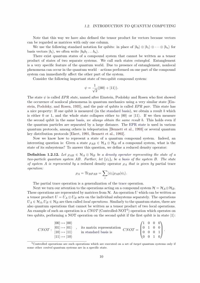
These operations are represented by matrices fromH. An operation U which can be written asa tensor product U = UA⊗UB acts on the individual subsystems separately. The operationsUA ∈ HA, UB ∈ HB are then called local operations. Similarly to the quantum states, there arealso quantum operations that cannot be written as a tensor product of two local operations.An example of such an operation is a CNOT (Controlled-NOT3) operation which operates ontwo qubits, performing a NOT operation on the second qubit if the first qubit is in state |1〉:

CNOT :

|00〉 7→ |00〉|01〉 7→ |01〉|10〉 7→ |11〉|11〉 7→ |10〉

, its matrix representationin standard basis is

CNOT =

1 0 0 00 1 0 00 0 0 10 0 1 0

.

3Controlled operations are such operations which are executed on a set of target quantum systems only ifsome other control quantum systems are in a specific state.

10

CHAPTER 1. INTRODUCTION

Mixed state evolution

We now describe the formalism used to describe evolution of a quantum system representedby the density matrix:

ρ =∑i

pi|φi〉〈φi|.

The evolution of a state ρ is described by an operator E : ρ 7→ ρ′ which satisfies:

• E is linear:ρ′ = E(ρ) =

∑i

piE(|φi〉〈φi|),

• If E is applied on a density matrix it yields again a density matrix. Informally thismeans that if an operation described by E is applied onto a valid system, we obtainagain a valid system. We hence require that E maps a positive matrix to a positivematrix, and preserves trace of the matrix ρ as both Tr ρ and Tr ρ′ are equal to one (bydefinition of a density matrix),

• If E is applied to a part ρA of a compound system ρAB then the compound systemremains in a valid state. In particular, it can be described by a density matrix. Thiscondition is called complete positivity.

Now we formalize the previous requirements.

Definition 1.2.13. Let HB be a Hilbert space. We call a linear operator F : HB −→ HB:

• trace-preserving if for for any positive matrix ρB ∈ HB, Tr ρB = Tr F (ρB),

• positive if for any positive matrix ρB ∈ HB, F (ρB) yields a positive matrix,

• completely positive if F is positive and for any positive matrix ρB ∈ HB, Hilbert spaceHA and a positive matrix ρAB ∈ HA ⊗HB such that TrA ρAB = ρB, (I ⊗ F )ρAB is apositive matrix.

A trace-preserving completely positive operator is called a superoperator.

The name superoperator was given because it transforms density operators to densityoperators.

Remark 1.2.14. Like for density matrices, the superoperator can be alternatively defined asa completely positive operator E such that for a density matrix A in the sense of Remark1.2.10, E is a completely positive operator where Tr E(A) ≤ Tr A.

The evolution of a closed quantum system is like in the case of pure states represented byan application of a unitary operator on its density matrix. However, as we do not apply thematrix to the vector but to a matrix, there is a difference: Should such a unitary operationU be applied to a density operator ρ, we represent it as a superoperator EU :

ρ′ = EU (ρ) = UρU †.

Superoperators can also represent evolution of open quantum systems, ie. quantum sys-tems which interact with other systems (environment) whose state is unknown. Such an

11

1.3. MODELS OF QUANTUM COMPUTATION

evolution is not necessary unitary. Let us have a pure state ρ and let the evolution be repre-sented by a superoperator E . Then the state E(ρ) can be mixed.

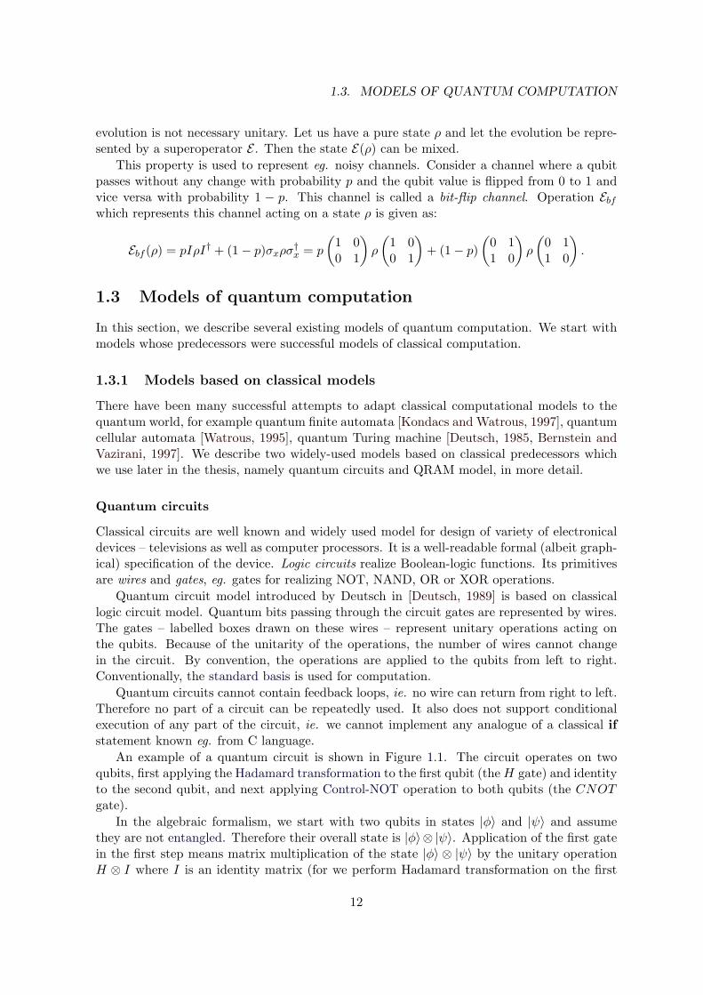
This property is used to represent eg. noisy channels. Consider a channel where a qubitpasses without any change with probability p and the qubit value is flipped from 0 to 1 andvice versa with probability 1 − p. This channel is called a bit-flip channel. Operation Ebfwhich represents this channel acting on a state ρ is given as:

Ebf (ρ) = pIρI† + (1− p)σxρσ†x = p

(1 00 1

)ρ

(1 00 1

)+ (1− p)

(0 11 0

)ρ

(0 11 0

).

1.3 Models of quantum computation

In this section, we describe several existing models of quantum computation. We start withmodels whose predecessors were successful models of classical computation.

1.3.1 Models based on classical models

There have been many successful attempts to adapt classical computational models to thequantum world, for example quantum finite automata [Kondacs and Watrous, 1997], quantumcellular automata [Watrous, 1995], quantum Turing machine [Deutsch, 1985, Bernstein andVazirani, 1997]. We describe two widely-used models based on classical predecessors whichwe use later in the thesis, namely quantum circuits and QRAM model, in more detail.

Quantum circuits

Classical circuits are well known and widely used model for design of variety of electronicaldevices – televisions as well as computer processors. It is a well-readable formal (albeit graph-ical) specification of the device. Logic circuits realize Boolean-logic functions. Its primitivesare wires and gates, eg. gates for realizing NOT, NAND, OR or XOR operations.

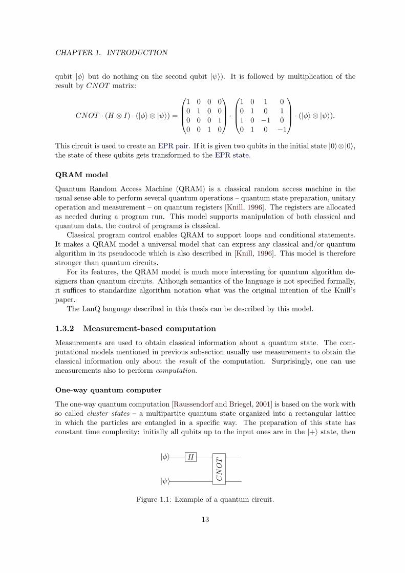
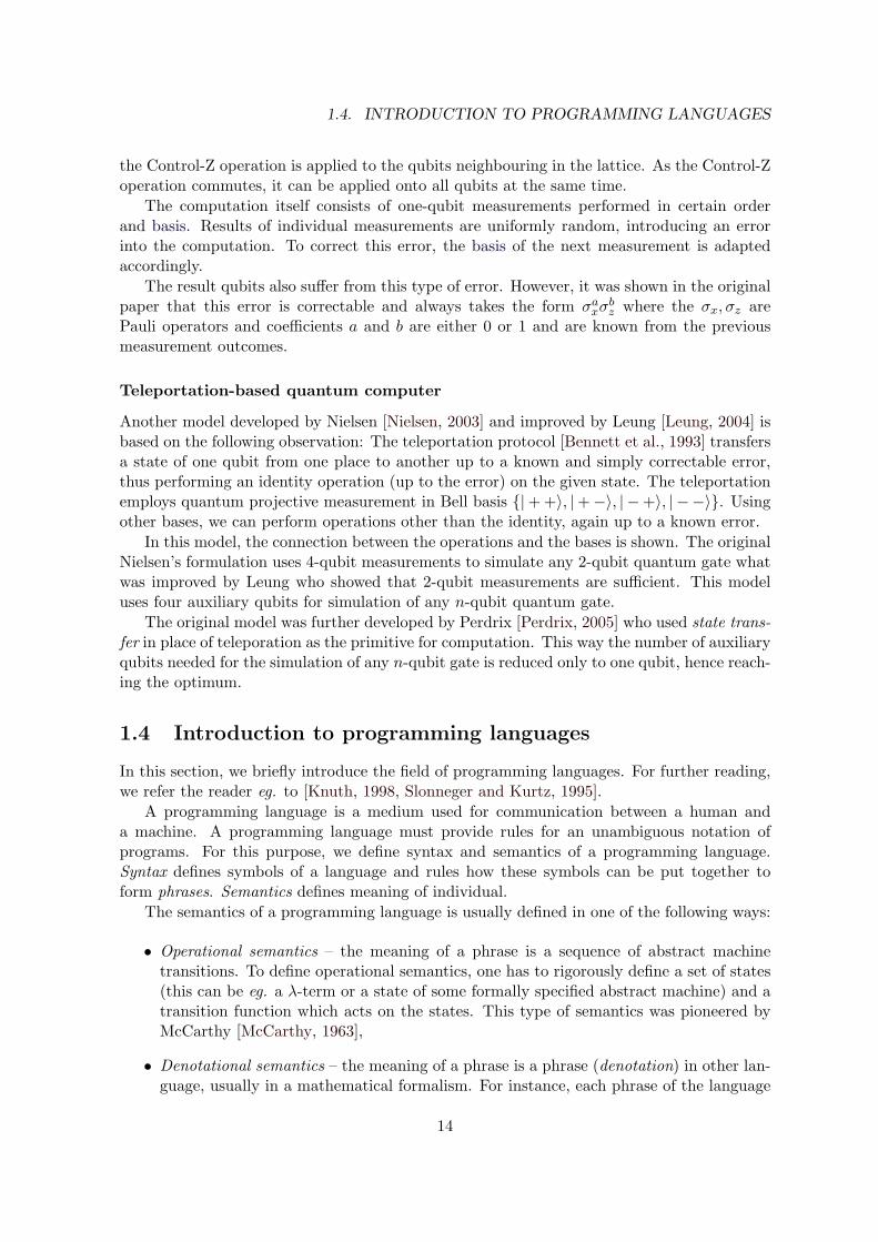
Quantum circuit model introduced by Deutsch in [Deutsch, 1989] is based on classicallogic circuit model. Quantum bits passing through the circuit gates are represented by wires.The gates – labelled boxes drawn on these wires – represent unitary operations acting onthe qubits. Because of the unitarity of the operations, the number of wires cannot changein the circuit. By convention, the operations are applied to the qubits from left to right.Conventionally, the standard basis is used for computation.

Quantum circuits cannot contain feedback loops, ie. no wire can return from right to left.Therefore no part of a circuit can be repeatedly used. It also does not support conditionalexecution of any part of the circuit, ie. we cannot implement any analogue of a classical ifstatement known eg. from C language.

An example of a quantum circuit is shown in Figure 1.1. The circuit operates on twoqubits, first applying the Hadamard transformation to the first qubit (theH gate) and identityto the second qubit, and next applying Control-NOT operation to both qubits (the CNOTgate).

In the algebraic formalism, we start with two qubits in states |φ〉 and |ψ〉 and assumethey are not entangled. Therefore their overall state is |φ〉⊗ |ψ〉. Application of the first gatein the first step means matrix multiplication of the state |φ〉 ⊗ |ψ〉 by the unitary operationH ⊗ I where I is an identity matrix (for we perform Hadamard transformation on the first

12

CHAPTER 1. INTRODUCTION

qubit |φ〉 but do nothing on the second qubit |ψ〉). It is followed by multiplication of theresult by CNOT matrix:

CNOT · (H ⊗ I) · (|φ〉 ⊗ |ψ〉) =

1 0 0 00 1 0 00 0 0 10 0 1 0

·

1 0 1 00 1 0 11 0 −1 00 1 0 −1

· (|φ〉 ⊗ |ψ〉).This circuit is used to create an EPR pair. If it is given two qubits in the initial state |0〉⊗|0〉,the state of these qubits gets transformed to the EPR state.

QRAM model

Quantum Random Access Machine (QRAM) is a classical random access machine in theusual sense able to perform several quantum operations – quantum state preparation, unitaryoperation and measurement – on quantum registers [Knill, 1996]. The registers are allocatedas needed during a program run. This model supports manipulation of both classical andquantum data, the control of programs is classical.

Classical program control enables QRAM to support loops and conditional statements.It makes a QRAM model a universal model that can express any classical and/or quantumalgorithm in its pseudocode which is also described in [Knill, 1996]. This model is thereforestronger than quantum circuits.

For its features, the QRAM model is much more interesting for quantum algorithm de-signers than quantum circuits. Although semantics of the language is not specified formally,it suffices to standardize algorithm notation what was the original intention of the Knill’spaper.

The LanQ language described in this thesis can be described by this model.

1.3.2 Measurement-based computation

Measurements are used to obtain classical information about a quantum state. The com-putational models mentioned in previous subsection usually use measurements to obtain theclassical information only about the result of the computation. Surprisingly, one can usemeasurements also to perform computation.

One-way quantum computer

The one-way quantum computation [Raussendorf and Briegel, 2001] is based on the work withso called cluster states – a multipartite quantum state organized into a rectangular latticein which the particles are entangled in a specific way. The preparation of this state hasconstant time complexity: initially all qubits up to the input ones are in the |+〉 state, then

|φ〉 H

CNOT

|ψ〉

Figure 1.1: Example of a quantum circuit.

13

1.4. INTRODUCTION TO PROGRAMMING LANGUAGES

the Control-Z operation is applied to the qubits neighbouring in the lattice. As the Control-Zoperation commutes, it can be applied onto all qubits at the same time.

The computation itself consists of one-qubit measurements performed in certain orderand basis. Results of individual measurements are uniformly random, introducing an errorinto the computation. To correct this error, the basis of the next measurement is adaptedaccordingly.

The result qubits also suffer from this type of error. However, it was shown in the originalpaper that this error is correctable and always takes the form σaxσ

bz where the σx, σz are

Pauli operators and coefficients a and b are either 0 or 1 and are known from the previousmeasurement outcomes.

Teleportation-based quantum computer

Another model developed by Nielsen [Nielsen, 2003] and improved by Leung [Leung, 2004] isbased on the following observation: The teleportation protocol [Bennett et al., 1993] transfersa state of one qubit from one place to another up to a known and simply correctable error,thus performing an identity operation (up to the error) on the given state. The teleportationemploys quantum projective measurement in Bell basis |+ +〉, |+−〉, | −+〉, | − −〉. Usingother bases, we can perform operations other than the identity, again up to a known error.

In this model, the connection between the operations and the bases is shown. The originalNielsen’s formulation uses 4-qubit measurements to simulate any 2-qubit quantum gate whatwas improved by Leung who showed that 2-qubit measurements are sufficient. This modeluses four auxiliary qubits for simulation of any n-qubit quantum gate.

The original model was further developed by Perdrix [Perdrix, 2005] who used state trans-fer in place of teleporation as the primitive for computation. This way the number of auxiliaryqubits needed for the simulation of any n-qubit gate is reduced only to one qubit, hence reach-ing the optimum.

1.4 Introduction to programming languages

In this section, we briefly introduce the field of programming languages. For further reading,we refer the reader eg. to [Knuth, 1998, Slonneger and Kurtz, 1995].

A programming language is a medium used for communication between a human anda machine. A programming language must provide rules for an unambiguous notation ofprograms. For this purpose, we define syntax and semantics of a programming language.Syntax defines symbols of a language and rules how these symbols can be put together toform phrases. Semantics defines meaning of individual.

The semantics of a programming language is usually defined in one of the following ways:

• Operational semantics – the meaning of a phrase is a sequence of abstract machinetransitions. To define operational semantics, one has to rigorously define a set of states(this can be eg. a λ-term or a state of some formally specified abstract machine) and atransition function which acts on the states. This type of semantics was pioneered byMcCarthy [McCarthy, 1963],

• Denotational semantics – the meaning of a phrase is a phrase (denotation) in other lan-guage, usually in a mathematical formalism. For instance, each phrase of the language

14

CHAPTER 1. INTRODUCTION

is associated a number or a function. The phrases can be combined to form biggerphrases according to the language syntax. The denotation of these bigger phrases isgiven by composing the denotations of their subphrases, therefore denotational seman-tics is compositional. This type of semantics was developed by Scott and Strachey [Scottand Strachey, 1971],

• Categorical semantics – the semantics of a phrase is given by a morphism in a categorywith prescribed properties. Categorical semantics is hence more abstract than the de-notational. The actual shape of the category can vary a lot – for example Abramskyand Coecke showed that quantum mechanics can be described by a strongly compactclosed category with biproducts [Abramsky and Coecke, 2004].4 As the category of finitevector spaces with unitary transformations, category of sets and relations and a planepicture calculus [Coecke, 2005] are such categories, they all can be used to interpretquantum theory.

There are also other approaches to semantics, among others: action semantics, algebraicsemantics, axiomatic semantics, game semantics. For further reading on semantics of pro-gramming languages, we refer the reader to [Slonneger and Kurtz, 1995] and to [Abramskyand McCusker, 1999] specifically for game semantics.

A paradigm of a programming language determines a way of expressing programs in thelanguage. The main paradigms are the following:

• Functional – a program is an expression written in a declarative form. The programresult is given by reduction of the expression,

• Logical – a program is a theory written in a declarative form. The program result is ananswer to some question. This answer has to satisfy the given theory,

• Imperative – a program is a description of a way to obtain a result. During a programrun, a global variable specifying a program state is updated.

An imperative programming language that supports definition of methods (or functions,routines, procedures) is called procedural. Methods are parametrized program fragments. Theyallow programmers to structure a program into smaller pieces of code. This improves read-ability of program code and makes it easier to maintain the program code. The program canthen invoke the methods from within a caller method. After a method finishes its execution,it eventually returns a return value to its caller.

A higher-order programming language allows one to manipulate functions as if they weredata. In such languages it is possible to create functions during a program run, functionscan return other functions as their return value etc. A language which is not higher-order iscalled first-order.

A variable in imperative languages is a specification of a memory location where a valueis stored. In functional languages, a variable denotes a variable in the usual mathematicalmeaning.

In general, it is possible to create syntactically correct terms that have no meaning. Toavoid this unwanted freedom, we add a type system to a language. A type of a variablespecifies a range of the valid values of the variable. Languages where variables are given

4Similar result was independently obtained by Selinger [Selinger, 2005].

15

1.4. INTRODUCTION TO PROGRAMMING LANGUAGES

a type are called typed [Cardelli, 2004]. To give an example of what typing is useful for,consider a type letter of letters of English alphabet. Let c denote a variable of type letter.Then c can stand for a letter “g” but it cannot represent a number 4. The usage of typesallows a compiler to detect such errors at compile-time. Therefore, taking c as in the previousexample, assignment of a value 4 to the variable c can be detected at compile-time and thiserror can be reported to the programmer.

Types are particularly useful when developing a programming language that allows theprogrammer to express combination of both quantum and classical computations. For exam-ple, quantum data cannot be in general duplicated (due to no-cloning theorem, [Wootters andZurek, 1982]), while classical data can. This means that classical and quantum data mustbe handled differently what can be achieved eg. by using different types for quantum andclassical variables.

Type soundness

A useful propery of typed languages is type soundness. A language with sound type systemguarantees that if a term in the language is typable (ie. we can infer a type of the term), thenthe evaluation of this term never terminates because of a type error5 (weak type soundness)[Milner, 1978].

We can often prove strong type soundness of a language which guarantees that the evalu-ation of a typable term t either diverges or yields an answer6 of the same type as the term t.Note that what several other authors, eg. [Cardelli, 2004], understand by type soundness isin fact strong type soundness.

Type soundness of a language is nowadays most usually proved using a technique byWright and Feleisen [Wright and Felleisen, 1994]. This technique is based on similar proofs ofsubject reduction from combinatory logic and on term rewriting as specified by operationalsemantics.

1.4.1 Quantum programming languages

A quantum programming language is a language that allows a programmer to describe com-putations in the quantum world and possibly also in the classical world. We can characterizeprogramming languages by “quantumness” of their control state and manipulated data.

Classical programs can be characterized by the slogan classical control, classical data:both control state of a program and data are classical.

Quantum programs can be characterized either by slogan quantum control, quantum dataor classical control, quantum data. Control state of a program in the former style is quantummeaning that it can be in a superposition of multiple basis states. In this case all the data arequantum. Programs in the latter style support manipulation of both quantum and classicaldata while employing a classical program control state. Note that this behaviour is exactlymodelled by a QRAM.

Several existing quantum programming languages are discussed in Chapter 2.

5A type error is a language-dependent concept usually meaning an error arising from passing such argumentsto a function which do not belong to the function domain, eg. attempt to add a number 7 to a boolean valuefalse.

6Specification of what the answer looks like is again language-dependent.

16

CHAPTER 1. INTRODUCTION

1.5 Introduction to process algebras

In this section, we briefly introduce the field of process algebras. For further reading, werefer the reader to [Fokkink, 2000] and [Bergstra, Ponse, and Smolka, 2001] for an in-depthintroduction to this field, and to [Baeten, 2004] for a historical overview.

A process describes behaviour of a system, ie. a sequence of observable actions andevents that are performed in the system. A process algebra is the study of behaviour ofparallel or distributed systems by algebraic means [Baeten, 2004]. It is a mathematical toolfor describing or specifying processes and their interactions and reasoning about them bymeans of equations. Hence, process algebras are crucial for proving different kinds of processequivalences and properties of multiparty protocols.

A process description consists of actions and their compositions. The set of actions isdependent on the system settings. An action can be for instance a keypress on a keyboardor an allocation of a resource. These actions can be composed together to form processes bymany different operators. The most common composition operators are:

• Sequential composition P1.P2 of two processes P1 and P2 – the process P2 is run afterthe process P1 is successfully completed,

• Alternative composition P1 +P2 of two processes P1 and P2 – the system nondetermin-istically executes either process P1 or P2

7,

• Parallel composition P1 ‖ P2 (or P1 |P2) of two processes P1 and P2 – the systemexecutes the processes P1 and P2 simultaneously,

• Probabilistic composition P1 pP2 of two processes P1 and P2 – the system executes theprocesses P1 with probability p or P2 with probability (1− p).

The most influential process algebras are Milner’s CCS (Calculus of Communicating Sys-tems) [Milner, 1980], CSP (Communicating Sequential Processes) by Hoare [Hoare, 1983] andACP (Algebra of Communicating Processes) by Bergstra and Klop [Bergstra and Klop, 1984].For further reading on these algebras, we refer the reader to [Baeten and Weijland, 1990] and[Bergstra et al., 2001].

The work of Milner, Parrow and Walker led to the development of π-calculus, a calculuswhere not only data but also communication channels can be passed over a channel from aprocess to another process [Milner, Parrow, and Walker, 1992]. This feature is used eg. tomodel a situation when a person A is travelling with a mobile phone while speaking to personB – while travelling, the phone changes its base stations during the call but the communicationchannel between A and B remains the same.

Any process algebra containing both nondeterministic and probabilistic choices has tospecify which choice is solved first. For more information on this account see [Cazorla, Cuar-tero, Ruiz, Pelayo, and Pardo, 2003].

Communication

The interaction between two or more processes is done by communication. Process algebrasoffer tools for describing communication among processes, usually by means of abstraction of

7Note that process algebras are inherently nondeterministic – the choice of order in which the concurrentprocesses evolve is nondeterministic.

17

1.5. INTRODUCTION TO PROCESS ALGEBRAS

communication links called channels. We distinguish two types of communication:

• Synchronous (blocking) communication – when a sender attempts to send a message,its execution is delayed until there is another process which can receive. Similarly,when a receiver attempts to receive a message, its execution is delayed until there isanother process which sends a message over the corresponding channel. This type ofcommunication can indeed lead to a deadlock when there is no sender/receiver to areceiving/sending process,

• Asynchronous (nonblocking) communication – a sent message “waits” in a channel untilthere is a receiver which can receive the message, the sender continues its executionwithout waiting for the receiver.

It has been proved that asynchronous communication can be simulated using the syn-chronous one but synchronous cannot be simulated using the asynchronous [Palamidessi,1997].

Note that communication can be a source of nondeterminism. Consider the following fourprocesses (we use the notation of π-calculus):

A(g) = g〈3〉.0 B(g) = g(x).0 C(g) = g(x).0 System = (νg)(A(g)|B(g)|C(g))

The process A sends a number 3 over the communication channel g and terminates. Bothprocesses B and C behave identically: After a successful reception of the number from thechannel g the process terminates. The process System allocates a channel g and executes theprocesses A,B and C in parallel. Now, which of the processes B or C receives the sent value3, is left to the nondeterminism.

This type of nondeterminism was recognized earlier and there were several approaches tohandle it. Kobayashi, Pierce and Turner suggest in [Kobayashi, Pierce, and Turner, 1996]using a linear type system over the π-calculus. A channel is assigned a polarity (whether itcan be used for sending or receiving) and multiplicity (how many times it can be used forcommunication, either 1 or ω). Linear channels are those channels whose multiplicity is 1regardless of their polarity. Type system then uses polarities to guarantee that linear channelsare used by at most two processes at a time, one sender and one receiver. For a solution for amore complex formalism where channel types for structured communication (so called sessiontypes) can be specified see eg. [Gay and Hole, 2005, Yoshida and Vasconcelos, 2007]. Thesolution is also based on channel polarities checked by the type system.

1.5.1 Quantum process algebras

In quantum process algebras, the communication and the manipulated data can be classicalor quantum. This has a large impact on quantum resource handling: a process calculus mustguarantee unique ownership of quantum systems among processes.

Moreover, if a quantum process algebra supports a combination of quantum and classicalcomputations, expression of quantum measurements must be allowed. Because the measure-ments are probabilistic by nature, it has to deal with probabilistic choice. As mentionedearlier, if the process algebra also supports nondeterministic choice, it must specify whichchoice – the probabilistic or the nondeterministic – is solved first when they occur simultane-ously.

18

Chapter 2

Current state of the art

In this chapter, we give a brief characterization of several quantum programming languagesand process algebras that have been developed so far. For the currently most complete surveyon quantum programming languages we refer the reader to [Gay, 2006] and to [Glendinning,2005] for an online list of them.

Some of the languages will be discussed in more detail in Chapter 10 where they will bealso compared with LanQ.

2.1 Functional languages and λ-calculi

We can view programs as descriptions of functions which transform input values to someoutput. This is one reason why many of proposed quantum programming languages arefunctional. Another reason why functional languages are so popular, is that their operationalsemantics can be straightforwardly defined.

λ-calculus is a mathematical formal system introduced by Church and Kleene in 1930s.It has a very simple and well-known syntax for writing expressions. Operational semanticsis straightforwardly given by reduction rules. Nevertheless, it is powerful enough to expressany computable function. Any functional language can be viewed as a syntactic variation ofthe λ-calculus [Slonneger and Kurtz, 1995]. This justifies the decision to put the functionallanguages and λ-calculi to the same section.

2.1.1 Quantum λq-calculus – van Tonder

The first successful attempt to create a functional quantum programming language was doneby Andre van Tonder in 2003 [van Tonder, 2003a]. He created untyped λ-calculus for quantumcomputing. He proved the model of this calculus to be computationally equivalent to quantumTuring machines. This λ-calculus was later extended to a typed λ-calculus in [van Tonder,2003b] where denotational semantics of the latter calculus was also developed.

The language supports higher-order computations to be expressed.To deal with quantum resources, techniques from a linear λ-calculus were employed. The

resources are divided into two groups:

• Linear – these resources can be neither copied nor discarded. Quantum states in theλq-calculus are considered to be linear resources,

19

2.1. FUNCTIONAL LANGUAGES AND λ-CALCULI

• Nonlinear – these resources can be both copied and discarded.

A disadvantage of the quantum λq-calculus is the nonexistence of measurements in the lan-guage. This constraint makes it impossible to combine classical and quantum computations.Therefore, this language can be used for describing purely quantum algorithms.

The simulator is available from http://www.het.brown.edu/people/andre/qlambda/.

2.1.2 QPL

Selinger’s QPL [Selinger, 2004] is an important typed functional language. This language canbe described by a slogan “quantum data, classical control”. It can be used to express anyalgorithm manipulating quantum and classical data or their combination.

The syntax of the language has two interchangeable forms. A program can be describedby a graphical flow chart. This form is intuitive and has direct connection to the semanticsbut it is difficult to manipulate and discourages structured programming. For this reason, astructured textual form of the language exists.

The linearity of quantum data is enforced by the syntax which ensures that syntacticallydistinct variables will refer to physically distinct objects. The language is very restrictive inhandling variables: eg. it denies to assign an expression or even a value of another variableto a variable. For example, if a and b are of type bit, the only way to set a to the value of bis the following: if b then a := 1 else a := 0. Indeed, this nonconformity can be overcomeby using syntactic abbreviations for frequently used statements.

QPL is the first quantum language with well-defined denotational semantics. The se-mantics is given by assigning any program fragment a generalized superoperator acting ongeneralized density matrix tuples: A generalized density matrix D is a positive matrix suchthat Tr D ≤ 1. A generalized density matrix tuple (D0, . . . , Dn) is a tuple of generalized den-sity matrices Di such that

∑ni=0 ≤ 1. A generalized superoperator that acts on generalized

density matrix tuples is then defined similarly to the usual definition of superoperator (see[Selinger, 2004]).

The generalization of the density matrix formalism is used to represent of finite classicaldata. The i-th element of a generalized density matrix tuple Di represents the state ofquantum world if the overall state of classical memory is represented by the number i. Theprobability that the classical memory is in overall state i is given by the trace Tr Di.

The fact that generalized superoperators form a complete partial order enables semanticsof loops and recursion to be defined naturally as a limit of a sequence of superoperators.

Selinger also defines a categorical semantics of the language. Later he showed in [Selinger,2005] the connection between the categorical semantics of [Abramsky and Coecke, 2004] andthe semantics of QPL.

2.1.3 QML

QML is a typed language developed by Altenkirch and Grattage [Altenkirch and Grattage,2004]. It supports both classical and quantum computations to be expressed. Both data andcontrol of the program flow may be quantum.

Even though the language is functional, it only supports first-order computations to beexpressed; all data types are finite. It is therefore not possible to treat functions as data.

The technique used for developing the language semantics is interesting. First, they lookat classical computations and show them to be reversible in a closed system. Then they

20

CHAPTER 2. CURRENT STATE OF THE ART

explain irreversible classical computations based on reversible mechanics. To show it theyutilize a heap. Heap is an auxiliary space which can be used during computation.

Let A,B be two finite sets. Reversible finite computation of a function f : A → B isrepresented by a bijection on finite sets: φf : A × H → B × G where G is a set of possibleheap states after computation and H is a set of possible heap states before computation. Suchtwo bijections φf , φg are considered extensionally equivalent if the functions f and g, whosereversible computations they represent, are equal (f = g). Any computable function f on afinite domain can be represented by such a mapping φf .

The authors justify usage of superoperators for definition of semantics of quantum com-putation in the following way: A superoperator can be represented by a space expansion,application of a unitary transformation in the larger space and finally tracing out the aux-iliary space. This gives a picture similar to that of the previous paragraph. Therefore, anyquantum computation should be in general represented by superoperators.

The authors put emphasis on the control of decoherence. For this purpose, their languageoffers two different if–then–else constructs. One of them measures a qubit in the condition,the second one does not. However, the second if-construct can be used only in certain cases.

Another tool used to control the decoherence is minimalisation of weakenings (ie. dis-carding of quantum states). This is achieved by the type system based on strict logic. Min-imalisation of weakenings is a difference to other quantum programming languages whichprevent contraction (duplication of a quantum system) to occur. Indeed, the language doesnot support duplication of quantum data, but two or more variables are allowed to refer tothe same quantum system.

The language compiler is available from http://sneezy.cs.nott.ac.uk/qml/compiler/.

2.1.4 Quantum λ-calculus – Selinger & Valiron

The calculus developed by Selinger and Valiron in [Selinger and Valiron, 2006] is a typed“quantum data, classical control” λ-calculus. Higher-order computations can be expressed inthis language. Contrary to van Tonder’s language, combination of both classical and quantumcomputations is supported, measurement of a quantum system is a primitive in the language.

To support handling of both quantum and classical data, the type system distinguishesbetween the types whose values are duplicable and whose not. This type system is used toguarantee that no-cloning and no-deleting of quantum data is not violated. Interestingly, thisnot only holds for the ground data types but also for the higher-order types. It is thereforepossible to have a function of type qbit −→ qbit that can be called only once and anotherthat can be invoked multiple times.

It is remarkable that the type system does not satisfy principal type property, ie. thatevery untyped expression has the most general type. Therefore the authors had to develop atype-inference algorithm which can determine whether a given term is typable in the lineartype system, and find its type.

The authors define operational semantics of this language in terms of probabilistic reduc-tion rules. They prove type preservation and progress lemmata for well-typed programs.

2.1.5 nQML

nQML [Lampis, Ginis, and Papaspyrou, 2006] is a language based on the previously describedQML language by Grattage and Altenkirch. This language is characterized by the slogan

21

2.2. OTHER LANGUAGES

“quantum data and control”, allowing to perform a measurement at any point during aprogram run.

The language supports variable aliasing hence several quantum variables can point to thesame qubit. To prevent a situation when one qubit is used more than once in one quantumoperation, the authors employ the type system. The type of quantum expressions containsspecification of the place of the qubits in which the expression value is stored. Then it is easyto check the requirement of distinctness of quantum variables without introducing linear typesystem.

Denotational semantics of the language is defined using density matrices in terms of uni-tary operations (for terms not containing measurements) and general functions from densitymatrices to density matrices (for those containing measurements).

A publicly available implementation exists and is available from ftp://ftp.softlab.ntua.gr/pub/users/nickie/papers/nqml06.code.tar.gz.

2.2 Other languages

2.2.1 qGCL

Quantum Guarded Command Language (qGCL) was developed by Sanders and Zuliani in[Sanders and Zuliani, 2000, Zuliani, 2001]. Both quantum and classical computations andtheir combination can be expressed. qGCL was developed from the probabilistic languagepGCL which, in turn, was created using Dijkstra’s GCL as a basis. pGCL was chosen as abase of qGCL because of its rigorous semantics.

A probabilistic guarded-command language program is a sequence of assignments andstatements skip and abort. The program is manipulated by standard constructors of se-quential composition with conditionals, loops and probabilistic and nondeterministic choice.A quantum program in qGCL is a pGCL program which uses quantum procedures. Thesequantum procedures can be of three types: initialisation of a quantum state, evolution andfinalisation (a measurement).

This language can be used both as a specification language and a programming language.It has well defined operational semantics. The refinement calculus associated with qGCL wasinherited from pGCL and extended. It allows systematic program derivation and algebraicreasoning about qGCL programs. The refinement calculus also allows to simplify programsalgebraically. Simplification is seen as a particular program refinement which preserves se-mantics.

Even though recursion is available in pGCL, the language qGCL does not support it[Zuliani, 2001, Sec. 2.4]. This was a decision during design of this language because of thecompilation technique used.

2.2.2 QCL

Imperative language QCL was designed by Omer in [Omer, 2000, 2003]. It supports bothquantum and classical computations to be expressed and freely interleaved. Its syntax isbased on that of C language what makes it easy to learn for ordinary programmers.

This language is interesting for many reasons. The language offers tools for simple defini-tion of a quantum operator in the language. It supports creation of reversible quantum gates

22

CHAPTER 2. CURRENT STATE OF THE ART

from classical-like code (so called quantum functions). This allows programmers with only arough knowledge of quantum mechanics to create quantum operators.

QCL is not a higher-order programming language, but it retains some features of higher-order languages. For example, it is possible to automatically compute an inverse of a quantumoperator.

The semantics of this language is not defined. Therefore, it is impossible to prove aprogram written in QCL to satisfy some property.

Omer developed a QCL simulator that is publicly available from http://tph.tuwien.ac.at/~oemer/qcl.html.

This language is further discussed in Section 10.2.

2.2.3 Q language

Betteli, Calarco and Serafini’s Q language [Bettelli, Calarco, and Serafini, 2001] is not alanguage written from scratch. It is an extension of the existing C++ language. Like QCL,it supports description of both quantum and classical computations and their combination.

Q philosophy is to extend existing standard language instead of creating a new one.This way programmers need not learn a new language, they just learn the extension.1 Thisapproach also allows the developers to use existing compilers for compilation of programswritten in Q. No new compilers or simulators need to be developed, it is possible to onlyextend the existing ones.

This language supports combination of quantum and classical computation in the sameway as in QRAM model. This means that classical computations are performed on a clas-sical computer; quantum device, that performs quantum computations, is controlled by theclassical computer.

Unitary operators are represented by objects in the sense of object-oriented programming.This representation allows programmers to create operators during a program run usingoperator composition, conjugation etc. Created operators can be optimised before they areused at the quantum device. If the quantum device does not support execution of arbitraryquantum operations, this approach allows the control machine to compute a decompositionof an operator to such primitives that the quantum device can perform.

The semantics of this language is not defined formally. A publicly available implementa-tion exists and is available from http://sra.itc.it/people/serafini/qlang/.

2.2.4 QMC

Quantum Model Checker by Gay, Nagarajan and Papanikolaou [Gay, Nagarajan, and Pa-panikolaou, 2007] is a single-process quantum model checker with a formally defined syntaxand semantics. It uses a subset of exogenous quantum propositional logic (EQPL) [Baltazar,Mateus, and Sernadas, 2007] to check the properties of the resulting state. The tool scansall possible paths which the execution of the checked program can take due to quantummeasurements and checks whether the EQPL formula is satisfied for all possible programruns.

The model-checker uses the stabilizer formalism for quantum system state representation.Note that using this formalism, instead of one state, a set of quantum states satisfying givenstabilizer equations is represented. Stabilizer formalism only allows us to use Clifford group

1This is the same idea that was used for development of the LanQ syntax.

23

2.3. QUANTUM PROCESS ALGEBRAS

operations, 1-qubit measurements, and Clifford group operations conditioned on classical bitsto be applied onto a quantum state. Although the set of operations is not universal and notall quantum states can be expressed in this formalism, this model is rich enough to expressmany practically usable algorithms and protocols, eg. teleportation protocol [Bennett et al.,1993] or quantum dense coding [Bennett and Wiesner, 1992]. Moreover, it is known to beefficiently simulable on classical computers (Gottesman-Knill Theorem, [Gottesman, 1998])and an algorithm for its simulation exists [Aaronson and Gottesman, 2004].

Both EQPL and stabilizer formalism limit the dimension of used quantum systems to two,hence only qubits can be used in the programs. Although it is an insuperable obstacle in awork with higher-dimensional quantum systems, this design decision has important impacton speed making the implementation very fast.

Currently, the number of qubits manipulated by the program must be specified before theprogram is run and cannot be changed during the execution. Although this decision of theauthors does not usually cause a problem, the algorithms which allocate qubits dynamicallyin a loop can be limited by this restriction.

The model checker implementation is under development.

2.3 Quantum process algebras

There have been developed several quantum process algebras. We describe two of them,QPAlg and CQP.

2.3.1 CQP

Communicating Quantum Processes developed in [Gay and Nagarajan, 2004, 2005, 2006] isanother quantum process algebra. It can describe both quantum and classical interactions andevolution of processes. The syntax and semantics of this algebra are based on the π-calculus.

In this algebra, the channels are dynamically allocated. Therefore, they are only availableto the allocating process and its subprocesses. However, the number of subprocesses that canuse an allocated channel for communication is not limited. This way three or more processescan use one channel hence introducing nondeterminism as described in Section 1.5.

Communication channels are typed. The type of values that can be sent over individualchannels is given by the type of the channel. For example, sending a value of type char overchannel that can send only values of type bit, is impossible.

The algebra guarantees unique quantum system ownership among processes. Contrary toQPAlg, type soundness is proved for the language. A typechecking algorithm exists and isproved to be sound and complete [Gay and Nagarajan, 2006].

This algebra is further discussed in Section 10.3.

2.3.2 QPAlg

The quantum process algebra QPAlg by Lalire and Jorrand [Lalire and Jorrand, 2004, Jor-rand and Lalire, 2004] can describe both classical and quantum interaction and evolution ofprocesses. The syntax and operational semantics of this algebra are based on that of CCS andLotos. Recently [Lalire, 2006a], it was enhanced by a fixpoint operator and typed channels.

Names of quantum variables are stored together with their state in a context. The stateof quantum variables used in any process in the system is represented by a density matrix.

24

CHAPTER 2. CURRENT STATE OF THE ART

The context is also used for storing a mapping between classical variables names and theirvalues. The context is formed in a style of a cactus stack what allows one to declare variablesshared among several processes.

Processes can communicate over named gates. The gates that processes can use forcommunication are static, ie. they are given before a process run. Hence, they need not beallocated before their usage. This means that any process has access to any channel until thechannels are hidden by a special handling construct.

The algebra defines a bisimilarity relation on processes (which is an equivalence relationon processes) in the sense of probabilistic branching bisimulation [Lalire, 2006b]. This type ofbisimilarity is weaker than strong bisimilarity because it abstracts from silent transitions.

This algebra is further discussed in Section 10.4.

2.4 Summary

All the programming languages presented in this chapter can be used for description of quan-tum algorithms. Some of the languages cannot describe combination of quantum and classi-cal computations (van Tonder’s λq-calculus). But a practically-usable programming languageshould support such a combination to be expressed. The reason is that in practice, users passclassical input to a program and require classical output to be returned. Therefore, a classicalpart of the program should process the input and invoke quantum computation. After thequantum computation is finished, it should present its output to the user in a classical form.

Functional languages regard programs as mathematical expressions. Functional programsare manipulated according to mathematical rules. Two of the described functional languagessupport quantum data processing, but the flow control is classical – Selinger and Valiron’sλ-calculus and Selinger’s QPL. Both languages require a quantum system to be referreduniquely, ie. at most one variable should refer to one quantum system. This is a very strongconstraint. In real programming, it is quite useful when two or more variables can refer toone quantum system. This constraint is overcome in the QML language by Altenkirch andGrattage and nQML by Lampis, Ginis and Papaspyrou. In their languages, it is allowed tohave two or more variables referring to a single quantum system.

Contrary to functional languages, imperative languages rather reflect underlying machinearchitecture. Even though functional languages have better formal basis, practical program-mers prefer imperative programming languages to functional ones.

The qGCL language can be used both as a specification language and a programminglanguage. Its well-defined semantics and refinement calculus make this program a good basefor optimisation tasks. However, this language lacks recursion.

QCL is quite a usable language. It allows programmer to encode nearly any algorithm,quantum or classical, in the language. It contains many usable features like scratch-spacemanagement. However, the semantics of the language is not fully defined. Therefore formalproving of program properties is impossible. This is also true for the Q language.

QMC is an imperative language that supports checking of EQPL formulas over stabilizerstates. Its speed makes it a good choice for verification of properties of quantum states evenin complex programs if these states and operations over them can be described in terms ofstabilizer formalism.

A programming language LanQ developed in the dissertation is imperative and has well-defined operational semantics. The semantics is an improvement over two of the mentioned

25

2.4. SUMMARY

imperative languages (QCL, Q-language). Moreover, it exhibits several features of processalgebras, being able to run several processes in parallel and supporting interprocess commu-nication. Its simulator has been implemented and is shortly described in Appendix B

26

Part II

LanQ programming language

27

Chapter 3

Introduction

In this part of the thesis, we formally define the language LanQ and prove its properties –unique resource ownership and type soundness. The presentation of the language is based onthe articles [Mlnarık, 2006a,b, 2007]. The part is structured as follows:

• In this chapter, we show an example of a LanQ program,

• The syntax is presented in Chapter 4,

• The typing system is introduced in Chapter 5,

• The concepts used in the language semantics definition are formalized in Chapter 6,

• The language operational semantics is defined in Chapter 7,

• The unique resource ownership property is proved in Chapter 8,

• Type soundness of LanQ is proved in Chapter 9,

• We provide a comparison of LanQ to other existing programming languages and processalgebras in Chapter 10.

3.1 Informal introduction

We begin our description of LanQ by an example of implementation of a well-known mul-tiparty quantum protocol – a teleportation of an unknown quantum state [Bennett et al.,1993].

First, we declare a method prep0 that prepares a new qubit initialized in the |0〉 stateand returns it as its result. This method is shown in Figure 3.1. It returns a qubit what isseen from the type qbit written in front of the method name. On the first line of the methodbody, a qubit variable q is declared. We then assign a newly allocated qubit initialized ina maximally mixed state to q. The qubit is then measured in the standard basis. If themeasurement result is 1, we know that the qubit q collapsed to the state |1〉, so we apply thePauli operator σx onto it to turn it to the |0〉 state. Otherwise, it collapsed into the required|0〉 state. Therefore q in both cases denotes a qubit in |0〉 state. The qubit is returned to thecaller by the return statement.

29

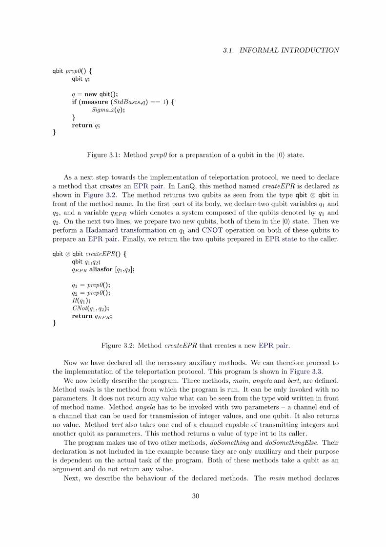
3.1. INFORMAL INTRODUCTION

qbit prep0() qbit q;

q = new qbit();if (measure (StdBasis,q) == 1)

Sigma x(q);return q;

Figure 3.1: Method prep0 for a preparation of a qubit in the |0〉 state.

As a next step towards the implementation of teleportation protocol, we need to declarea method that creates an EPR pair. In LanQ, this method named createEPR is declared asshown in Figure 3.2. The method returns two qubits as seen from the type qbit ⊗ qbit infront of the method name. In the first part of its body, we declare two qubit variables q1 andq2, and a variable qEPR which denotes a system composed of the qubits denoted by q1 andq2. On the next two lines, we prepare two new qubits, both of them in the |0〉 state. Then weperform a Hadamard transformation on q1 and CNOT operation on both of these qubits toprepare an EPR pair. Finally, we return the two qubits prepared in EPR state to the caller.

qbit ⊗ qbit createEPR() qbit q1,q2;qEPR aliasfor [q1,q2];

q1 = prep0();q2 = prep0();H(q1);CNot(q1, q2);return qEPR;

Figure 3.2: Method createEPR that creates a new EPR pair.

Now we have declared all the necessary auxiliary methods. We can therefore proceed tothe implementation of the teleportation protocol. This program is shown in Figure 3.3.

We now briefly describe the program. Three methods, main, angela and bert, are defined.Method main is the method from which the program is run. It can be only invoked with noparameters. It does not return any value what can be seen from the type void written in frontof method name. Method angela has to be invoked with two parameters – a channel end ofa channel that can be used for transmission of integer values, and one qubit. It also returnsno value. Method bert also takes one end of a channel capable of transmitting integers andanother qubit as parameters. This method returns a value of type int to its caller.

The program makes use of two other methods, doSomething and doSomethingElse. Theirdeclaration is not included in the example because they are only auxiliary and their purposeis dependent on the actual task of the program. Both of these methods take a qubit as anargument and do not return any value.

Next, we describe the behaviour of the declared methods. The main method declares

30

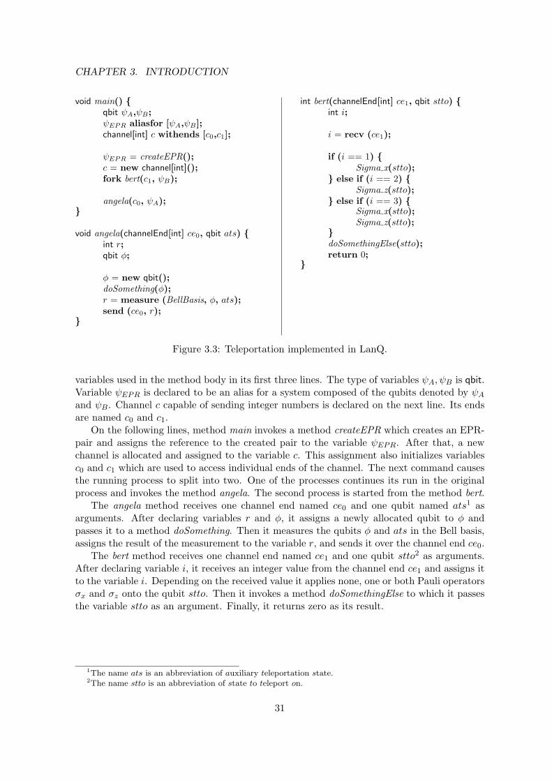
CHAPTER 3. INTRODUCTION

void main() qbit ψA,ψB;ψEPR aliasfor [ψA,ψB];channel[int] c withends [c0,c1];

ψEPR = createEPR();c = new channel[int]();fork bert(c1, ψB);

angela(c0, ψA);

void angela(channelEnd[int] ce0, qbit ats) int r;qbit φ;

φ = new qbit();doSomething(φ);r = measure (BellBasis, φ, ats);send (ce0, r);

int bert(channelEnd[int] ce1, qbit stto) int i;

i = recv (ce1);

if (i == 1) Sigma x(stto);

else if (i == 2) Sigma z(stto);

else if (i == 3) Sigma x(stto);Sigma z(stto);

doSomethingElse(stto);return 0;

Figure 3.3: Teleportation implemented in LanQ.

variables used in the method body in its first three lines. The type of variables ψA, ψB is qbit.Variable ψEPR is declared to be an alias for a system composed of the qubits denoted by ψAand ψB. Channel c capable of sending integer numbers is declared on the next line. Its endsare named c0 and c1.

On the following lines, method main invokes a method createEPR which creates an EPR-pair and assigns the reference to the created pair to the variable ψEPR. After that, a newchannel is allocated and assigned to the variable c. This assignment also initializes variablesc0 and c1 which are used to access individual ends of the channel. The next command causesthe running process to split into two. One of the processes continues its run in the originalprocess and invokes the method angela. The second process is started from the method bert.

The angela method receives one channel end named ce0 and one qubit named ats1 asarguments. After declaring variables r and φ, it assigns a newly allocated qubit to φ andpasses it to a method doSomething. Then it measures the qubits φ and ats in the Bell basis,assigns the result of the measurement to the variable r, and sends it over the channel end ce0.

The bert method receives one channel end named ce1 and one qubit stto2 as arguments.After declaring variable i, it receives an integer value from the channel end ce1 and assigns itto the variable i. Depending on the received value it applies none, one or both Pauli operatorsσx and σz onto the qubit stto. Then it invokes a method doSomethingElse to which it passesthe variable stto as an argument. Finally, it returns zero as its result.

1The name ats is an abbreviation of auxiliary teleportation state.2The name stto is an abbreviation of state to teleport on.

31

3.1. INFORMAL INTRODUCTION

32

Chapter 4

Syntax

In this chapter, we define concrete syntax of LanQ programs, internal syntax used for rep-resentation of a parsed program, and syntax of configurations that are used for definition ofoperational semantics of the language.

4.1 Concrete syntax

In this section, we introduce concrete syntax of LanQ programs. This syntax is used to writeprograms like the one in Figure 3.3 by a programmer.

The syntax is shown in Figure 4.1. Reserved words of the language are written in boldand the identifier names are in capitals. Grammar is given in nondeterministic extendedBackus-Naur form (EBNF). The root of the grammar is the nonterminal program.

For the sake of clarity, the concrete grammar nonterminals names are long and descrip-tive to indicate their meaning in semantics. We describe meaning of the most importantnonterminals here:

• program – words derived from this nonterminal represent LanQ programs,

• code – words derived from this nonterminal represent statements,

• pExpr – words derived from this nonterminal represent promotable expressions, ie.those expressions that can act as statements when they are suffixed with a semicolon,

• methodCall – words derived from this nonterminal represent method calls,

• assignment – words derived from this nonterminal represent assignments to variables,

• measurement – words derived from this nonterminal represent quantum measurements,

• expr – words derived from this nonterminal represent expressions,

• indivExpr – words derived from this nonterminal represent ground expressions, ie.expressions that do not contain any operators,

• op – words derived from this nonterminal represent mathematical operators,

• method – words derived from this nonterminal represent method declarations,

33

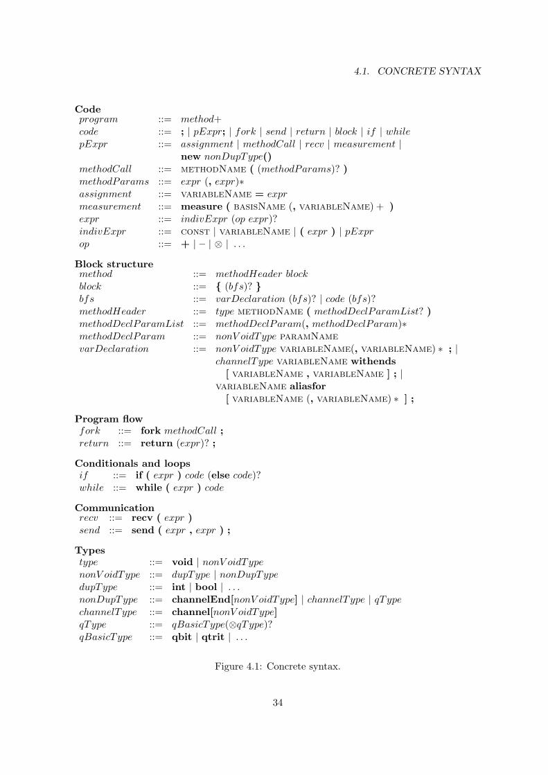
4.1. CONCRETE SYNTAX

Codeprogram ::= method+code ::= ; | pExpr; | fork | send | return | block | if | whilepExpr ::= assignment | methodCall | recv | measurement |

new nonDupType()methodCall ::= methodName ( (methodParams)? )methodParams ::= expr (, expr)∗assignment ::= variableName = exprmeasurement ::= measure ( basisName (, variableName) + )expr ::= indivExpr (op expr)?indivExpr ::= const | variableName | ( expr ) | pExprop ::= + | – | ⊗ | . . .

Block structuremethod ::= methodHeader blockblock ::= (bfs)? bfs ::= varDeclaration (bfs)? | code (bfs)?methodHeader ::= type methodName ( methodDeclParamList? )methodDeclParamList ::= methodDeclParam(, methodDeclParam)∗methodDeclParam ::= nonV oidType paramNamevarDeclaration ::= nonV oidType variableName(, variableName) ∗ ; |

channelType variableName withends[ variableName , variableName ] ; |

variableName aliasfor[ variableName (, variableName) ∗ ] ;

Program flowfork ::= fork methodCall ;return ::= return (expr)? ;

Conditionals and loopsif ::= if ( expr ) code (else code)?while ::= while ( expr ) code

Communicationrecv ::= recv ( expr )send ::= send ( expr , expr ) ;

Typestype ::= void | nonV oidTypenonV oidType ::= dupType | nonDupTypedupType ::= int | bool | . . .nonDupType ::= channelEnd[nonV oidType] | channelType | qTypechannelType ::= channel[nonV oidType]qType ::= qBasicType(⊗qType)?qBasicType ::= qbit | qtrit | . . .

Figure 4.1: Concrete syntax.

34

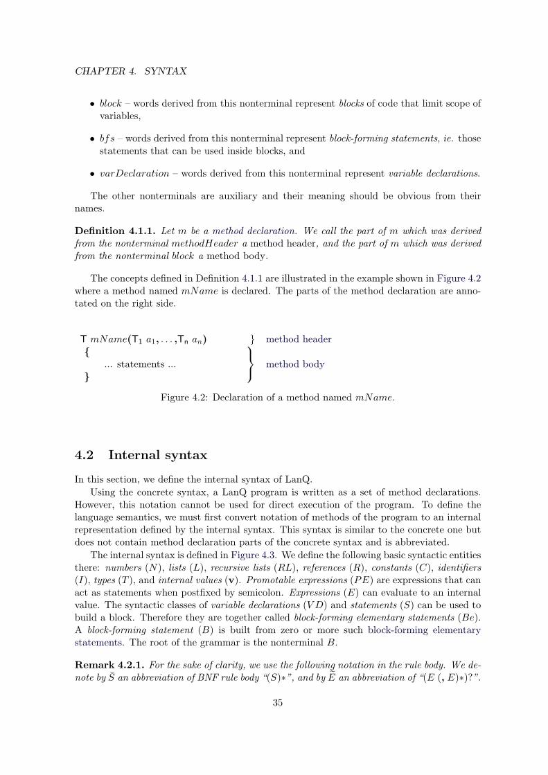
CHAPTER 4. SYNTAX

• block – words derived from this nonterminal represent blocks of code that limit scope ofvariables,

• bfs – words derived from this nonterminal represent block-forming statements, ie. thosestatements that can be used inside blocks, and

• varDeclaration – words derived from this nonterminal represent variable declarations.

The other nonterminals are auxiliary and their meaning should be obvious from theirnames.

Definition 4.1.1. Let m be a method declaration. We call the part of m which was derivedfrom the nonterminal methodHeader a method header, and the part of m which was derivedfrom the nonterminal block a method body.

The concepts defined in Definition 4.1.1 are illustrated in the example shown in Figure 4.2where a method named mName is declared. The parts of the method declaration are anno-tated on the right side.

T mName(T1 a1, . . . ,Tn an) method header

... statements ...

method body

Figure 4.2: Declaration of a method named mName.

4.2 Internal syntax

In this section, we define the internal syntax of LanQ.Using the concrete syntax, a LanQ program is written as a set of method declarations.

However, this notation cannot be used for direct execution of the program. To define thelanguage semantics, we must first convert notation of methods of the program to an internalrepresentation defined by the internal syntax. This syntax is similar to the concrete one butdoes not contain method declaration parts of the concrete syntax and is abbreviated.

The internal syntax is defined in Figure 4.3. We define the following basic syntactic entitiesthere: numbers (N), lists (L), recursive lists (RL), references (R), constants (C), identifiers(I), types (T ), and internal values (v). Promotable expressions (PE) are expressions that canact as statements when postfixed by semicolon. Expressions (E) can evaluate to an internalvalue. The syntactic classes of variable declarations (V D) and statements (S) can be used tobuild a block. Therefore they are together called block-forming elementary statements (Be).A block-forming statement (B) is built from zero or more such block-forming elementarystatements. The root of the grammar is the nonterminal B.

Remark 4.2.1. For the sake of clarity, we use the following notation in the rule body. We de-note by S an abbreviation of BNF rule body “(S)∗”, and by E an abbreviation of “(E (, E)∗)?”.

35

4.3. CONFIGURATION SYNTAX

N ::= 0 | 1 | . . .L ::= [] | [N ]RL ::= L | [RL]R ::= none | (Classical,N) | (Quantum,RL) | (Channel,N) |

(ChannelEnd0,N) | (ChannelEnd1,N) | (GQuantum,L) | (GChannel,N)C ::= R | true | false | ⊥ | . . .I ::= x | y | z | . . . | + | − | . . .T ::= void | int | qbit | channel[T ] | channelEnd[T ] | T ⊗ T | . . .v ::= 〈〈R,C〉〉T

PE ::= new T () | I = E | I(E) | measure(E) | recv(E)E ::= I | v | (E) | PEV D ::= T I; | channel[T ] I withends[I,I]; | I aliasfor [I];S ::= ; | PE; | B | if (E) S else S | while (E) S |

return; | return E; | fork I(E); | send(E,E);Be ::= V D | SB ::= Be

Figure 4.3: Internal syntax.

The semantics uses internal representation of the method bodies. Fortunately, the bodiesderived using the concrete syntax and those derived by the internal syntax rules differ onlyin the following:

• In internal representation, all if statements have else part, ie. a statement if (E) P isrewritten to if (E) P else ;,

• In internal representation, all constants C are represented by internal values 〈〈none, C〉〉Twhere T is the type of the constant C,

• In internal representation, all operators are written in the prefix notation and seen asmethod calls, ie. E F is converted to (E,F ).

There is obviously an algorithm which rewrites any method body derived using the con-crete syntax to the internal representation. The conversion can be performed right in theprogram parsing phase.

An example of a block written using the concrete syntax and its internal representationis shown in Figure 4.4.

4.3 Configuration syntax

Last, we must define the syntax of configurations that allows us to specify language semanticsin terms of their rewritings. The internal syntax is a part of the configuration syntax.

The configuration syntax specifies formal notation of configurations used for the definitionof the operational semantics of LanQ. It is shown in Figure 4.5. The root of the configurationsyntax is the nonterminal MConf . Meaning of individual configuration elements is describedlater in Section 7.3, examples of configurations can be found in Appendix A.

36

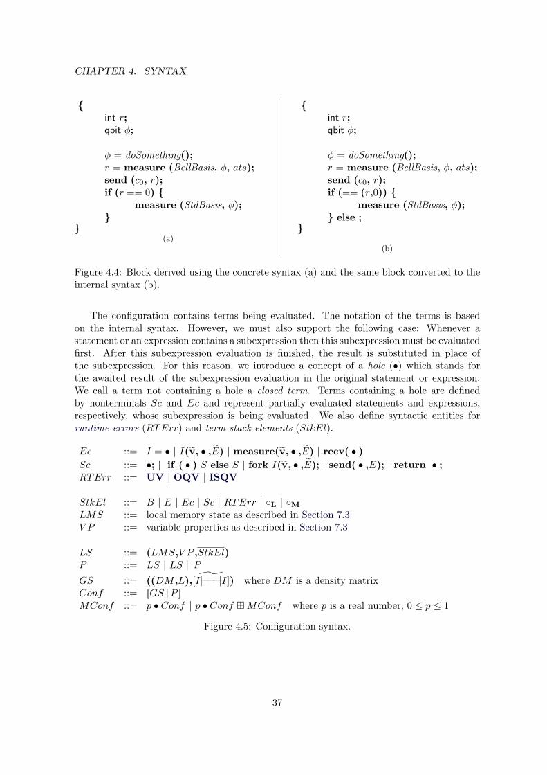
CHAPTER 4. SYNTAX

int r;qbit φ;

φ = doSomething();r = measure (BellBasis, φ, ats);send (c0, r);if (r == 0)

measure (StdBasis, φ);

(a)

int r;qbit φ;

φ = doSomething();r = measure (BellBasis, φ, ats);send (c0, r);if (== (r,0))

measure (StdBasis, φ); else ;

(b)

Figure 4.4: Block derived using the concrete syntax (a) and the same block converted to theinternal syntax (b).

The configuration contains terms being evaluated. The notation of the terms is basedon the internal syntax. However, we must also support the following case: Whenever astatement or an expression contains a subexpression then this subexpression must be evaluatedfirst. After this subexpression evaluation is finished, the result is substituted in place ofthe subexpression. For this reason, we introduce a concept of a hole (•) which stands forthe awaited result of the subexpression evaluation in the original statement or expression.We call a term not containing a hole a closed term. Terms containing a hole are definedby nonterminals Sc and Ec and represent partially evaluated statements and expressions,respectively, whose subexpression is being evaluated. We also define syntactic entities forruntime errors (RTErr) and term stack elements (StkEl).

Ec ::= I = • | I(v, • ,E) | measure(v, • ,E) | recv( • )Sc ::= •; | if ( • ) S else S | fork I(v, • ,E); | send( • ,E); | return • ;RTErr ::= UV | OQV | ISQV

StkEl ::= B | E | Ec | Sc | RTErr | L | MLMS ::= local memory state as described in Section 7.3V P ::= variable properties as described in Section 7.3

LS ::= (LMS,V P ,StkEl)P ::= LS | LS ‖ PGS ::= ((DM ,L),[ ˜I|== |=I]) where DM is a density matrixConf ::= [GS |P ]MConf ::= p • Conf | p • Conf MConf where p is a real number, 0 ≤ p ≤ 1

Figure 4.5: Configuration syntax.

37

4.3. CONFIGURATION SYNTAX

38

Chapter 5

Typing

5.1 Typing rules

LanQ is a typed language. This feature enables us to detect errors arising from incorrectusage of methods, variables and constants at compile time.

First, we define the ground types used in LanQ:

• void – a type with only one value: ⊥,1

• int – a type of integers,

• bool – a type of truth values true and false,

• qdit – a type of references to d-dimensional quantum systems. These types are calledquantum types. Types which are often used are given special names: one can write qbitinstead of writing q2it, and in place of q3it one can use qtrit,

• Q1 ⊗ Q2 – if Q1,Q2 are quantum types referring to d1, d2-dimensional systems, respec-tively, then Q1 ⊗ Q2 is a type of references to d1 · d2-dimensional quantum systems.These types are also called quantum types,

• channel[T] – if T is a ground type, it is a type of references to a channel capable oftransmitting values of type T. These types are called channel types,

• channelEnd[T] – if T is a ground type, it is a type of references to a channel end of achannel capable of transmitting values of type T.

The ground type system can be indeed extended when needed. Additionally, we use severalinternal types which cannot be used by the programmer:

• Ref – a type of references, defined later in Section 7.1,

• RTErr – a type of runtime errors, and

• MeasurementBasis – a type of measurement bases.1This type is a unit type. In several other languages, it is called differently, eg. unit in OCaml or () in

Haskell. We have decided to use the name void as usual in C-based languages because LanQ follows C languagealso in many other aspects.

39

5.1. TYPING RULES

Let S1, ...,Sn,S be ground types for n ≥ 0. Then a method type T is defined to be the typeS1,S2, ...,Sn → S. We call the types S1, . . . ,Sn argument types and the type S a return type.

Definition 5.1.1. We define a set Types of types of classical values. We denote by val(T) aset of values of type T and define a set V alues as a set of values of all types:

V alues =⋃

T∈Typesval(T).

After parsing a program, the method declarations are stored in a triplet (MT ,MH ,MB)of partial functions. We call this triplet a method typing context where:

• MT (m) which returns the method type for a method m (the method type is straight-forwardly determined from the method header),

• MH(m) returns the method header for a method m, and

• MB(m) which returns the method body represented in the internal syntax for a methodm.

We provide typechecking rules in Figures 5.1 (rules for typechecking programs), 5.2 (rulesfor typechecking variable declarations), 5.3 (rules for typechecking statements), and 5.4 (rulesfor typechecking expressions). All the typechecking rules use a typing context what is a pair(M ; Γ) consisting of:

• M is a method typing context,

• Γ is a variable typing context – a partial mapping Γ : Names Types that assigns atype to a variable name. We write a variable typing context Γ as Γ = a1 : T1, . . . , an : Tn

meaning that the type Ti is assigned to the variable ai.

The extension of a context Γ by a variable b of type Tb is written as Γ, b : Tb. It isundefined if b ∈ dom Γ and Γ(b) 6= Tb. Otherwise it is defined as:

(Γ, b : Tb)(x) =

Tb if x = b,

Γ(x) otherwise.

The rule T-Program is used to check typing of a program P whose internal representationis stored in a method typing context (MT ,MH ,MB). We call this program well-typed if thepremise of the rule T-Program is satisfied for all methods in this method typing context.This check is passed iff all the declared methods satisfy the premises of the typing rule T-Method.

Typechecking of a method in the rule T-Method is a little more complicated. The reasonis that we require any method m whose return type is not void to return a value of appropriatetype in all possible control paths which the evaluation of this method can take.

This can be checked at compile time. We split this requirement into two:

(1) during evaluation, the method m body always reaches a return statement (or invokesa runtime error or diverges or gets stuck due to incorrect send/recv pairing), and

40

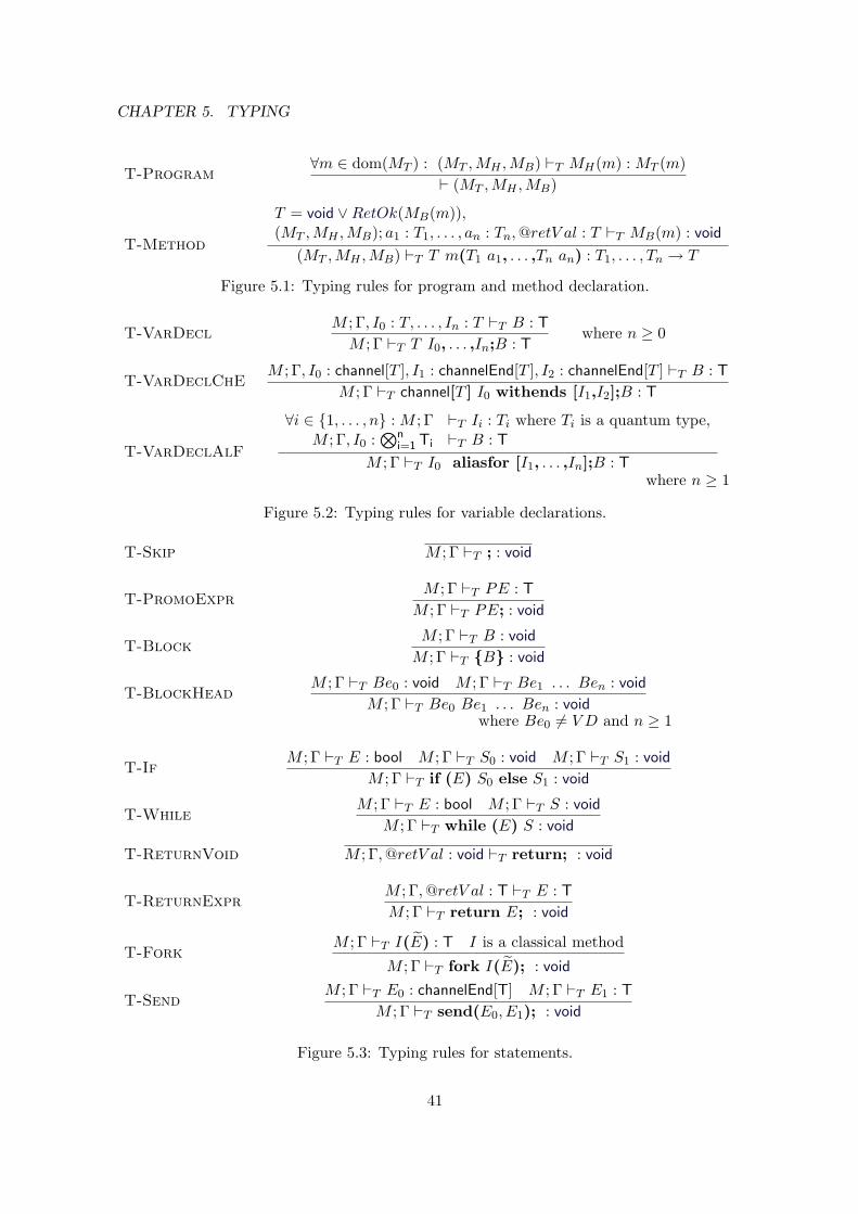
CHAPTER 5. TYPING

T-Program∀m ∈ dom(MT ) : (MT ,MH ,MB) `T MH(m) : MT (m)

` (MT ,MH ,MB)

T-Method

T = void ∨RetOk(MB(m)),(MT ,MH ,MB); a1 : T1, . . . , an : Tn,@retV al : T `T MB(m) : void

(MT ,MH ,MB) `T T m(T1 a1, . . . ,Tn an) : T1, . . . , Tn → T

Figure 5.1: Typing rules for program and method declaration.

T-VarDeclM ; Γ, I0 : T, . . . , In : T `T B : T

M ; Γ `T T I0, . . . ,In;B : Twhere n ≥ 0

T-VarDeclChEM ; Γ, I0 : channel[T ], I1 : channelEnd[T ], I2 : channelEnd[T ] `T B : T

M ; Γ `T channel[T ] I0 withends [I1,I2];B : T

T-VarDeclAlF

∀i ∈ 1, . . . , n : M ; Γ `T Ii : Ti where Ti is a quantum type,M ; Γ, I0 :

⊗ni=1 Ti `T B : T

M ; Γ `T I0 aliasfor [I1, . . . ,In];B : Twhere n ≥ 1

Figure 5.2: Typing rules for variable declarations.

T-Skip M ; Γ `T ; : void

T-PromoExprM ; Γ `T PE : T

M ; Γ `T PE; : void

T-BlockM ; Γ `T B : void

M ; Γ `T B : void

T-BlockHeadM ; Γ `T Be0 : void M ; Γ `T Be1 . . . Ben : void

M ; Γ `T Be0 Be1 . . . Ben : voidwhere Be0 6= V D and n ≥ 1

T-IfM ; Γ `T E : bool M ; Γ `T S0 : void M ; Γ `T S1 : void

M ; Γ `T if (E) S0 else S1 : void

T-WhileM ; Γ `T E : bool M ; Γ `T S : void

M ; Γ `T while (E) S : void

T-ReturnVoid M ; Γ,@retV al : void `T return; : void

T-ReturnExprM ; Γ,@retV al : T `T E : T

M ; Γ `T return E; : void

T-ForkM ; Γ `T I(E) : T I is a classical method

M ; Γ `T fork I(E); : void

T-SendM ; Γ `T E0 : channelEnd[T] M ; Γ `T E1 : T

M ; Γ `T send(E0, E1); : void

Figure 5.3: Typing rules for statements.

41

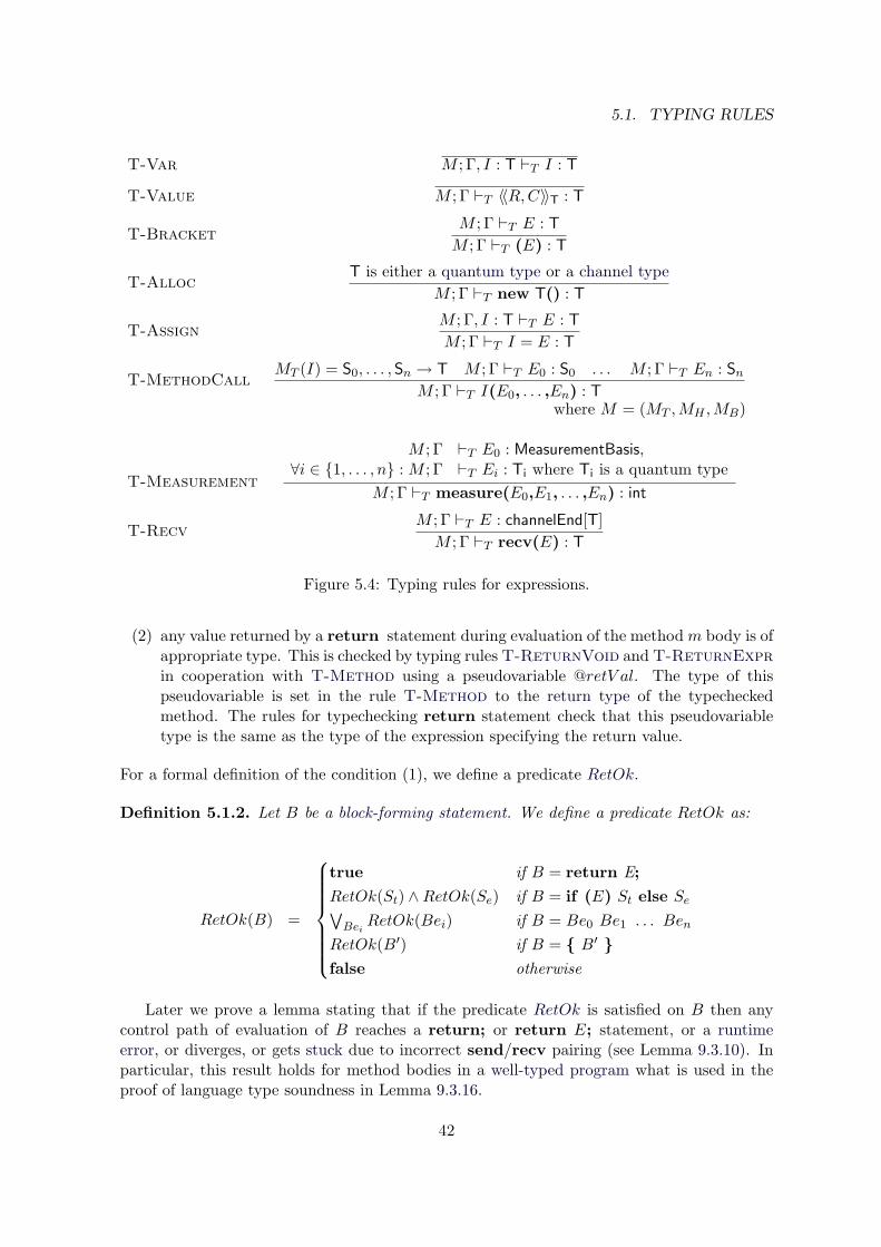
5.1. TYPING RULES

T-Var M ; Γ, I : T `T I : T

T-Value M ; Γ `T 〈〈R,C〉〉T : T

T-BracketM ; Γ `T E : T

M ; Γ `T (E) : T

T-AllocT is either a quantum type or a channel type

M ; Γ `T new T() : T

T-AssignM ; Γ, I : T `T E : T

M ; Γ `T I = E : T

T-MethodCallMT (I) = S0, . . . ,Sn → T M ; Γ `T E0 : S0 . . . M ; Γ `T En : Sn

M ; Γ `T I(E0, . . . ,En) : Twhere M = (MT ,MH ,MB)

T-Measurement

M ; Γ `T E0 : MeasurementBasis,∀i ∈ 1, . . . , n : M ; Γ `T Ei : Ti where Ti is a quantum type

M ; Γ `T measure(E0,E1, . . . ,En) : int

T-RecvM ; Γ `T E : channelEnd[T]M ; Γ `T recv(E) : T

Figure 5.4: Typing rules for expressions.

(2) any value returned by a return statement during evaluation of the method m body is ofappropriate type. This is checked by typing rules T-ReturnVoid and T-ReturnExprin cooperation with T-Method using a pseudovariable @retV al. The type of thispseudovariable is set in the rule T-Method to the return type of the typecheckedmethod. The rules for typechecking return statement check that this pseudovariabletype is the same as the type of the expression specifying the return value.

For a formal definition of the condition (1), we define a predicate RetOk.

Definition 5.1.2. Let B be a block-forming statement. We define a predicate RetOk as:

RetOk(B) =

true if B = return E;RetOk(St) ∧RetOk(Se) if B = if (E) St else Se∨Bei

RetOk(Bei) if B = Be0 Be1 . . . Ben

RetOk(B′) if B = B′ false otherwise

Later we prove a lemma stating that if the predicate RetOk is satisfied on B then anycontrol path of evaluation of B reaches a return; or return E; statement, or a runtimeerror, or diverges, or gets stuck due to incorrect send/recv pairing (see Lemma 9.3.10). Inparticular, this result holds for method bodies in a well-typed program what is used in theproof of language type soundness in Lemma 9.3.16.

42

CHAPTER 5. TYPING

Note that the predicate RetOk is only approximate. For example, it does not han-dle the case B = while (E) S because evaluation of the condition E is in general un-decidable at compile-time. Hence even for the straightforwardly always-terminating caseB = while (true) return 1;, RetOk(B) is not satisfied.

Definition 5.1.3. We call a method m well-typed if the premises of rule T-Method aresatisfied for this method.

Remark 5.1.4. Note that if a method m is well-typed and its return type is not void then itsbody contains only return E; statements, ie. no return; statements.

The rest of the typing rules is defined as usual: The rules for typechecking variable decla-rations in Figure 5.2 check that the subsequent block-forming statement can be typecheckedwith the variable context extended with the newly declared variables.

We formally regard all statements to be of type void what can be seen in the rules fortypechecking statements in Figure 5.3. These rules are quite usual up to the rule T-Fork.This rule requires that the method, which should be a new process run from, is classical. Thisis indeed a natural requirement as running a new process, which is by its nature a classicalobject, from a quantum operator would be a nonsense.

The rules for typechecking expressions shown in Figure 5.4 are designed as usual.

43

5.1. TYPING RULES

44

Chapter 6

Basic concepts

Before we continue with formal definition of the semantics, we must define several usefulfunctions and structures. First we define notation used in the rest of the thesis.

6.1 Notation

Notation 6.1.1. Let S be a set, ⊥ /∈ S. Then S⊥ = S ∪ ⊥. We denote a set of naturalnumbers with zero N ∪ 0 by N0.

Definition 6.1.2. Let S be a set. An S-list s = [s1, . . . , sn] is a list where n ∈ N0 ands1, . . . , sn ∈ S. Set of all finite S-lists s | s is a finite S-list is denoted by S[].

Definition 6.1.3. Let m,n ∈ N0. Let L = [l1, . . . , ln],K = [k1, . . . , km] be lists. Then |L|is a length of a list L, |L| = n. Concatenation of lists L and K is defined as L · K =[l1, . . . , ln, k1, . . . , km]. Set of list L elements is defined as set(L) = l1, . . . , ln.

6.2 Reference-related concepts

We use the following specially formed lists for storing references to quantum systems.

Definition 6.2.1. Let S be a set. We define a recursive S-list recursively as:

• Any S-list [s1, . . . , sk] is a recursive S-list,

• A list [e1, . . . , em] is a recursive S-list for any m ∈ N0 if e1, . . . , em are recursive S-lists.

For example, [[[1, 2, 3], [2, 3]], [1]] and [] are recursive N-lists.Recursive S-lists are used for the representation of quantum system references in the

following way: A reference to a quantum system, be it compound or not, is specified by arecursive N-list. Quantum systems are stored in indexed registers in the quantum memory,one quantum system per one register. The (unique) index is assigned to a quantum systemwhen it is allocated. The reference to the system with index n is a recursive N-list [n].

Let us have two quantum systems φ and ψ whose indices are 1 and 2, respectively. Thereferences to these quantum systems are rφ = [1] and rψ = [2], respectively. A reference to acompound system ρ consisting of the two quantum systems φ and ψ is then a recursive N-listrρ = [rφ, rψ] = [[1], [2]]. Note that the structure of ρ, ie. that it consists of two systems,corresponds to the structure of the reference rρ – it is built up from two elements.

45

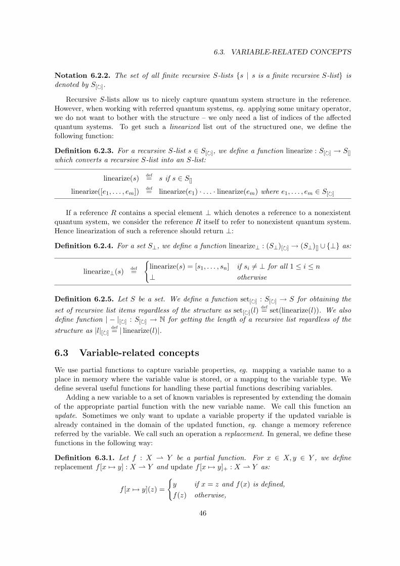
6.3. VARIABLE-RELATED CONCEPTS

Notation 6.2.2. The set of all finite recursive S-lists s | s is a finite recursive S-list isdenoted by S[].

Recursive S-lists allow us to nicely capture quantum system structure in the reference.However, when working with referred quantum systems, eg. applying some unitary operator,we do not want to bother with the structure – we only need a list of indices of the affectedquantum systems. To get such a linearized list out of the structured one, we define thefollowing function:

Definition 6.2.3. For a recursive S-list s ∈ S[], we define a function linearize : S[] → S[]

which converts a recursive S-list into an S-list:

linearize(s) def= s if s ∈ S[]

linearize([e1, . . . , em]) def= linearize(e1) · . . . · linearize(em) where e1, . . . , em ∈ S[]

If a reference R contains a special element ⊥ which denotes a reference to a nonexistentquantum system, we consider the reference R itself to refer to nonexistent quantum system.Hence linearization of such a reference should return ⊥:

Definition 6.2.4. For a set S⊥, we define a function linearize⊥ : (S⊥)[] → (S⊥)[] ∪ ⊥ as:

linearize⊥(s) def=

linearize(s) = [s1, . . . , sn] if si 6= ⊥ for all 1 ≤ i ≤ n⊥ otherwise

Definition 6.2.5. Let S be a set. We define a function set[] : S[] → S for obtaining the

set of recursive list items regardless of the structure as set[](l)def= set(linearize(l)). We also

define function | − |[] : S[] → N for getting the length of a recursive list regardless of the

structure as |l|[]def= | linearize(l)|.

6.3 Variable-related concepts

We use partial functions to capture variable properties, eg. mapping a variable name to aplace in memory where the variable value is stored, or a mapping to the variable type. Wedefine several useful functions for handling these partial functions describing variables.

Adding a new variable to a set of known variables is represented by extending the domainof the appropriate partial function with the new variable name. We call this function anupdate. Sometimes we only want to update a variable property if the updated variable isalready contained in the domain of the updated function, eg. change a memory referencereferred by the variable. We call such an operation a replacement. In general, we define thesefunctions in the following way:

Definition 6.3.1. Let f : X Y be a partial function. For x ∈ X, y ∈ Y , we definereplacement f [x 7→ y] : X Y and update f [x 7→ y]+ : X Y as:

f [x 7→ y](z) =

y if x = z and f(x) is defined,f(z) otherwise,

46

CHAPTER 6. BASIC CONCEPTS

and

f [x 7→ y]+(z) =

y if x = z,f(z) otherwise.

Note that the f [x 7→ y](x) is defined iff f(x) is defined while f [x 7→ y]+(x) is defined evenif f(x) is not defined.1

We need to store different variable properties: variable type, names of channel ends corre-sponding to a given channel etc. Each property is represented by a separate partial mapping.Hence variable properties are described by a tuple of such partial functions.

Definition 6.3.2. A partial function tuple is a tuple f = (f0, . . . , fn) where f0, . . . , fn arepartial functions.

We will need to capture variable scope during a method evaluation. For this reason,we define concepts of list of partial function tuples and list of lists of partial function tuples.Their usage is in more detail explained in Section 7.2. We also extend update and replacementfunctions to lists of partial function tuples and lists of lists of partial function tuples.

Definition 6.3.3. We define list of partial function tuples recursively as:

• is an (empty) list of partial function tuples,

• [K L f ] is a list of partial function tuples if K is a list of partial function tuples and fis a partial function tuple. The symbol L serves as an element separator only.2

Definition 6.3.4. For a list of partial function tuples K, we define a replacement K[x 7→ y]iand an update K[x 7→ y]+,i of outermost x in an i-th partial function of a list of partialfunction tuples K as:

[K1 L (f0, . . . , fn)][x 7→ y]idef=

[K1 L (f0, . . . , fi[x 7→ y], . . . , fn)] if fi(x) is defined[K1[x 7→ y]i L (f0, . . . , fn)] otherwise

[x 7→ y]idef=

[K1 L (f0, . . . , fn)][x 7→ y]+,idef= [K1 L (f0, . . . , fi[x 7→ y]+, . . . , fn)]

[x 7→ y]+,idef=

Definition 6.3.5. We define a list of lists of partial function tuples recursively as:

• is an (empty) list of lists of partial function tuples,

• [L1 G K] is a list of lists of partial function tuples if L1 is a list of lists of partialfunction tuples and K is a list of partial function tuples. The symbol G serves as anelement separator only.3

1The + sign in function index means “add the mapping from x to y even if it was not defined yet”.2L in L stands for local.3G in G stands for global.

47

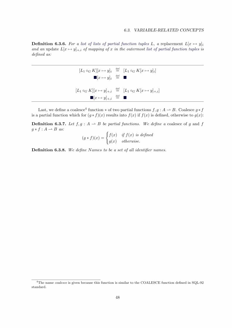
6.3. VARIABLE-RELATED CONCEPTS

Definition 6.3.6. For a list of lists of partial function tuples L, a replacement L[x 7→ y]iand an update L[x 7→ y]+,i of mapping of x in the outermost list of partial function tuples isdefined as:

[L1 G K][x 7→ y]idef= [L1 G K[x 7→ y]i]

[x 7→ y]idef=

[L1 G K][x 7→ y]+,idef= [L1 G K[x 7→ y]+,i]

[x 7→ y]+,idef=

Last, we define a coalesce4 function ∗ of two partial functions f, g : A B. Coalesce g ∗fis a partial function which for (g ∗ f)(x) results into f(x) if f(x) is defined, otherwise to g(x):

Definition 6.3.7. Let f, g : A B be partial functions. We define a coalesce of g and fg ∗ f : A B as:

(g ∗ f)(x) =

f(x) if f(x) is definedg(x) otherwise.

Definition 6.3.8. We define Names to be a set of all identifier names.

4The name coalesce is given because this function is similar to the COALESCE function defined in SQL-92standard.

48

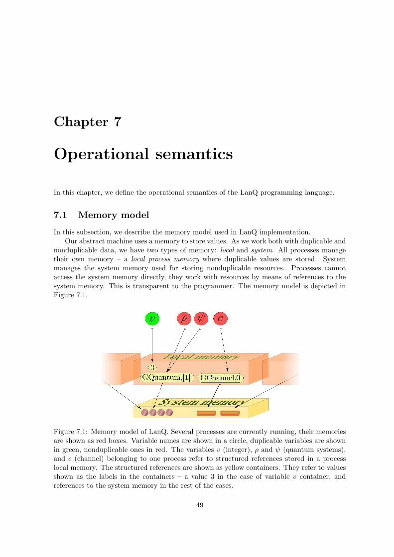
Chapter 7

Operational semantics

In this chapter, we define the operational semantics of the LanQ programming language.

7.1 Memory model

In this subsection, we describe the memory model used in LanQ implementation.Our abstract machine uses a memory to store values. As we work both with duplicable and

nonduplicable data, we have two types of memory: local and system. All processes managetheir own memory – a local process memory where duplicable values are stored. Systemmanages the system memory used for storing nonduplicable resources. Processes cannotaccess the system memory directly, they work with resources by means of references to thesystem memory. This is transparent to the programmer. The memory model is depicted inFigure 7.1.

Figure 7.1: Memory model of LanQ. Several processes are currently running, their memoriesare shown as red boxes. Variable names are shown in a circle, duplicable variables are shownin green, nonduplicable ones in red. The variables v (integer), ρ and ψ (quantum systems),and c (channel) belonging to one process refer to structured references stored in a processlocal memory. The structured references are shown as yellow containers. They refer to valuesshown as the labels in the containers – a value 3 in the case of variable v container, andreferences to the system memory in the rest of the cases.

49

7.1. MEMORY MODEL

This memory model consists of four layers. From bottom, the first layer is the systemmemory layer where the quantum systems and channels are physically stored. The next oneis a value layer which stores classical values and references to system memory. One layer up isa structured reference layer which stores references to the value layer. The structured referencelayer is particularly used for handling compound quantum systems. To topmost layer is thevariable layer which contains variable names. The connection between neighbouring layers isdone via three types of partial functions described later in Section 7.3.

This memory model allows us to assign a reference to the same nonduplicable resource tomany different variables. It also allows us to simply define communication of resources – themapping from a local reference (stored in the structured reference layer) to a global referenceto system memory (stored in the value layer) is invalidated in the sending process and createdat the receiver. It is however also a possible source of runtime errors. Consider a situationwhen a process sends away a qubit. Then the appropriate reference to the system memoryis removed but the mappings from variables to the local process memory are preserved. Ifa process then tries to use such a variable, a runtime error signalling uninitialized variableusage occurs.1

A memory reference specifies a position of a value in the memory. We distinguish twobasic types of references:

• Local references specify places in a local process memory where variable values arestored. The references assigned to variables during evaluation are always local. Aspecial local reference none refers to no place in the memory. We have four kinds oflocal references:

– References to local classical value memory: RefCl = none∪ (Classical×N⊥),

– References to local quantum system reference memory:RefQ = none ∪ (Quantum × (N⊥)[]),

– References to local channel reference memory: RefCh = none∪(Channel×N),

– References to local channel end reference memory:RefChE = none ∪ (ChannelEnd0, ChannelEnd1 × N).

The set of local references is defined as:

RefL = RefCl ∪RefQ ∪RefCh ∪RefChE .

• Global references refer to resources stored in system memory.

– References to system channel memory: RefGCh = ⊥ ∪ (GChannel × N⊥),

– References to system quantum memory: RefGQ = ⊥ ∪ (GQuantum × N[]).

1Note that the same behaviour would be exhibited if we invalidated the references from variable layer tothe structured reference layer. In that case, we would have to deinitialize all the variables referring to theresource. However, an invalidated variable could be used later in the program what would again lead to aruntime error.

We decided to unmap the references to the system memory layer because this operation is faster in general –the number of mappings from variable layer to structured reference layer is in general greater than the numberof mappings from the value layer to the structured reference layer.

50

CHAPTER 7. OPERATIONAL SEMANTICS

The set of global references is defined as:

RefG = RefGCh ∪RefGQ.

A set of all references is defined as:

Ref = RefG ∪RefL,

and a set of references to nonduplicable values is denoted by:

Refnd = RefQ ∪RefCh ∪RefChE .

Definition 7.1.1. A memory reference is an element from the set Ref . We define Ref to bethe type of memory references.

Remark 7.1.2. Note that a memory reference is a classical value, therefore Ref ∈ Types.

7.2 Variable properties storage

In this section, we informally introduce a structure used for handling variable properties.Variable properties is a structure where properties of variables neccessary for correct

handling of the variables are stored while respecting their scope: The actually running methodhas access only to variables declared in this method, it cannot access any variable from thecaller method. Moreover, the validity of a variable is limited to the block in which the variableis declared.

The properties of a variable are formally described later in Section 7.3. They are repre-sented by partial functions which, given a variable name, return:

• A reference to local process memory where the value of the variable is stored,

• Variable names representing individual ends of the channel (if the given variable repre-sents a channel),

• List of variable names representing quantum systems which are subsystems of the com-pound quantum system (if the given variable represents a compound quantum system),

• A type of the given variable.

Therefore we have a quadruple of partial functions that represent variable properties:f = (fvar, fch, fqa, ftype). Indeed, this quadruple alone is not powerful enough to handlevariable scope.

Respecting a variable scope is achieved by using lists of partial function tuples and listsof such lists:

• A variable can be accessed only from within the block where it was declared. This isensured by using a list of partial function tuples (separated by L), where a new tupleis appended to the list when a block is started and removed when the block ends,

• Only variables from the currently running method are accessible to this method. Thisis ensured by using a list of lists of partial function tuples (separated by G) where anew list of partial function tuples is appended when a method is invoked, and removedwhen the method finishes.

51

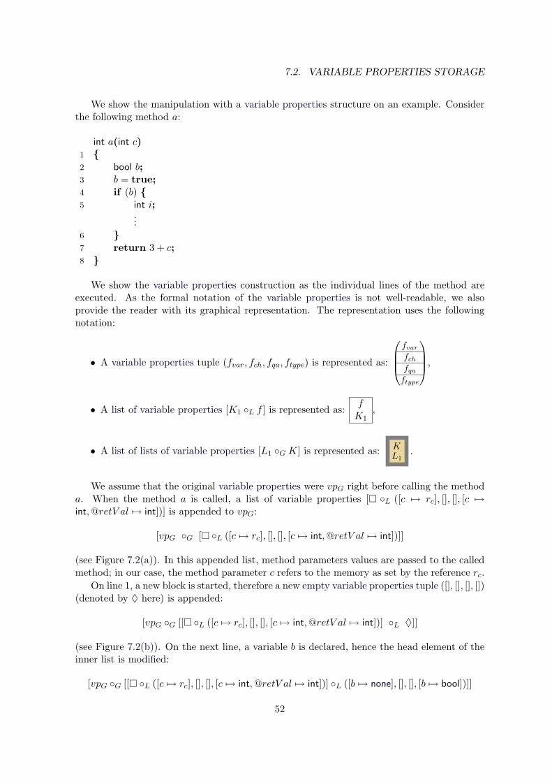
7.2. VARIABLE PROPERTIES STORAGE

We show the manipulation with a variable properties structure on an example. Considerthe following method a:

int a(int c)1 2 bool b;3 b = true;4 if (b) 5 int i;

...6 7 return 3 + c;8

We show the variable properties construction as the individual lines of the method areexecuted. As the formal notation of the variable properties is not well-readable, we alsoprovide the reader with its graphical representation. The representation uses the followingnotation:

• A variable properties tuple (fvar, fch, fqa, ftype) is represented as:

fvar

fch

fqa

ftype

,

• A list of variable properties [K1 L f ] is represented as:fK1

,

• A list of lists of variable properties [L1 G K] is represented as: K

L1

.

We assume that the original variable properties were vpG right before calling the methoda. When the method a is called, a list of variable properties [ L ([c 7→ rc], [], [], [c 7→int,@retV al 7→ int])] is appended to vpG:

[vpG G [ L ([c 7→ rc], [], [], [c 7→ int,@retV al 7→ int])]]

(see Figure 7.2(a)). In this appended list, method parameters values are passed to the calledmethod; in our case, the method parameter c refers to the memory as set by the reference rc.

On line 1, a new block is started, therefore a new empty variable properties tuple ([], [], [], [])(denoted by ♦ here) is appended:

[vpG G [[ L ([c 7→ rc], [], [], [c 7→ int,@retV al 7→ int])] L ♦]]

(see Figure 7.2(b)). On the next line, a variable b is declared, hence the head element of theinner list is modified:

[vpG G [[ L ([c 7→ rc], [], [], [c 7→ int,@retV al 7→ int])] L ([b 7→ none], [], [], [b 7→ bool])]]

52

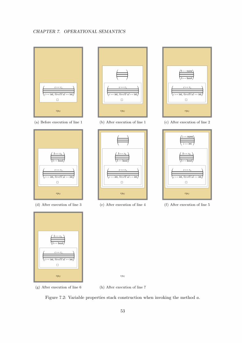
CHAPTER 7. OPERATIONAL SEMANTICS

vpG

c 7→ rc

c 7→ int, @retV al 7→ int

(a) Before execution of line 1

vpG

c 7→ rc

c 7→ int, @retV al 7→ int

(b) After execution of line 1

vpG

c 7→ rc

c 7→ int, @retV al 7→ int

b 7→ none

b 7→ bool

(c) After execution of line 2

vpG

c 7→ rc

c 7→ int, @retV al 7→ int

b 7→ rb

b 7→ bool

(d) After execution of line 3

vpG

c 7→ rc

c 7→ int, @retV al 7→ int

b 7→ rb

b 7→ bool

(e) After execution of line 4

vpG

i 7→ none

i 7→ int

c 7→ rc

c 7→ int, @retV al 7→ int

b 7→ rb

b 7→ bool

(f) After execution of line 5

vpG

c 7→ rc

c 7→ int, @retV al 7→ int

b 7→ rb

b 7→ bool

(g) After execution of line 6

vpG

(h) After execution of line 7

Figure 7.2: Variable properties stack construction when invoking the method a.

53

7.3. CONFIGURATION

(see Figure 7.2(c)). On line 3, b is assigned a value true which is stored in the memory ina place referred by a reference rb. This modifies fvar element of the appropriate variableproperties tuple:

[vpG G [[ L ([c 7→ rc], [], [], [c 7→ int,@retV al 7→ int])] L ([b 7→ rb], [], [], [b 7→ bool])]]

(see Figure 7.2(d)). On line 4, a new block is started, therefore again a new empty variableproperties tuple ♦ is appended:

[vpG G [[[ L ([c 7→ rc], [], [], [c 7→ int,@retV al 7→ int])] L ([b 7→ rb], [], [], [b 7→ bool])] L ♦]]

(see Figure 7.2(e)). On line 5, a new integer variable i is declared what is reflected in thehead variable properties tuple of the inner list:

[vpG G [[[ L ([c 7→ rc], [], [], [c 7→ int,@retV al 7→ int])] L ([b 7→ rb], [], [], [b 7→ bool])] L([i 7→ none], [], [], [i 7→ int])]]

(see Figure 7.2(f)). On line 6, the block ends, hence the appropriate variable properties tupleis discarded:

[vpG G [[ L ([c 7→ rc], [], [], [c 7→ int,@retV al 7→ int])] L ([b 7→ rb], [], [], [b 7→ bool])]]

(see Figure 7.2(g)). Finally on line 7, the method execution ends, hence all local variableproperties tuples are discarded and the original variable properties structure is restored:

vpG

(see Figure 7.2(h)).

7.3 Configuration

In this subsection, we formally define abstract machine configuration which is later used forthe definition of LanQ operational semantics.

A configuration of the abstract machine used for the definition of LanQ operational se-mantics is composed of two basic parts – global and local. The global part of the configurationrepresents system memory – a quantum state of the whole system and a relation betweenchannels and their ends. The local part of the configuration stores information about indi-vidual processes – the state of their local memory, variables, and terms to be evaluated.

A configuration C describing n processes running in parallel is written as:

C = [gs | ls1 ‖ · · · ‖ lsn]

where gs is the global part of the configuration and lsj represents the local process configu-ration of j-th process. The parallel composition ‖ is associative in LanQ, hence the pairwisebracketing of processes is not necessary.

The components of the abstract machine configuration are formally defined as follows:

• Global part of the configuration which describes the state of a system memory layer isa pair (Q,C) where:

54

CHAPTER 7. OPERATIONAL SEMANTICS

– Q describes the state of quantum particles and their dimensions.In the present paper, we represent the quantum state of the system by a pair(ρ, L) of a finite density matrix ρ and a finite list L of natural numbers. The listL represents dimensions of individual quantum subsystems. The order of the listelements is given by the order of quantum system allocations,

– C represents the channel part of the configuration.Channels and their ends are stored as pairs (c0, c1) written as c0|== |=

c1 where c0and c1 represent individual ends of one channel.

• Local part of the configuration: it defines the state of one process, hence we call it alocal process configuration. It is a triplet (lms, vp, ts) where:

– Local memory state lms is a quadruple of partial functions, lms = (lmsCl, lmsQ,lmsCh, lmsChE) which stores the state of classical memory and references to nondu-plicable resources available to the process:

∗ lmsCl : RefCl V alues is a partial function which returns a (classical) valuestored at the given position in memory. The set of all such partial functionsis denoted by LMSCl,

∗ lmsQ : RefQ RefGQ returns a global reference to quantum systems givenby the local quantum reference. The set of all such partial functions is denotedby LMSQ,

∗ lmsCh : RefCh RefGCh returns a global reference to the channel given bythe local channel reference. The set of all such partial functions is denoted byLMSCh,

∗ lmsChE : RefChE RefGCh returns a global reference to the channel corre-sponding to the given local channel end reference. The set of all such partialfunctions is denoted by LMSChE .

The local memory state connects the structured reference layer to the value layer.To simplify the notation, we regard lms itself as a partial function. Note thatRefGQ ⊆ V alues and RefGCh ⊆ V alues. Now we can define lms = (lmsCl, lmsQ,lmsCh, lmsChE) : RefL V alues as:

lms(r) =

lmsCl(r) if r ∈ RefCl,lmsQ(r) if r ∈ RefQ,lmsCh(r) if r ∈ RefCh,lmsChE(r) if r ∈ RefChE ,⊥ if r = none.

The set of all such quadruples lms is denoted by LMS.

– Variable properties vp represent various properties of variables while respectingvariable scope. They are stored as a list of lists of partial function tuples f =(fvar, fch, fqa, ftype) where:

∗ fvar : Names RefL maps a variable name to a local reference. This partialmapping is used to connect the variable layer to the structured reference layer,

55

7.4. VARIABLE PROPERTIES HANDLING FUNCTIONS

∗ fch : Names Names × Names maps a channel variable name to variablenames representing ends of the channel,

∗ fqa : Names Names[] maps a variable name representing a quantum systemto variable names that represent its subsystems,∗ ftype : Names Types maps a variable name to the variable type.

We call the quadruple f a variable properties tuple.We define V arPropL to be a set of all finite lists of such partial function tuplesf . These lists are built to reflect the block structure of a method as described inSection 7.2.We define V arProp to be a set of all finite lists of lists of such partial functiontuples f . These lists are built to reflect the method calls as described in Section 7.2.We define an empty variable properties tuple as a partial function tuple ♦:

♦ = (fvar, fch, fqa, ftype)

where dom(fvar) = dom(fch) = dom(fqa) = dom(ftype) = ∅.– Term stack ts: stack of terms to be evaluated. For the sake of readability, we use

a notation where individual stack items are underlined. An empty term stack isdenoted by ε.

A configuration can evolve to a probabilistic distribution over configurations, so calledmixed configuration. A mixed configuration:

pi, [gsi | lsi,1 ‖ · · · ‖ lsi,n]qi=1

is written as:

qi=1pi • [gsi | lsi,1 ‖ · · · ‖ lsi,n] where

q∑i=1

pi = 1.

It represents configurations of q different computational branches, each of them running withprobability pi. A configuration can be seen as a special case of a mixed configuration whereq = 1 and p1 = 1.

7.4 Variable properties handling functions

In this subsection, we define functions for retrieving information about variables using variableproperties.

The defined functions are designed so that they only work with variables accessible fromthe actually running method. We achieve this by inspecting the structure of the variableproperties. If the variable properties are represented by a list of lists of partial functiontuples L = [L1 G K] then we consider only its second element – the list of partial functiontuples K. We do not consider the variable properties from L1 as they are inaccessible to thecurrent method (as explained in Section 7.2).

We then walk through the obtained list of partial function tuples K = [K1 L f ]. Weattempt to get the requested information about requested variable using appropriate partialfunction from the variable properties tuple. If the requested information about the variablecannot be obtained from the actual tuple f , we repeat this procedure with the list of partialfunction tuples K1. This procedure is designed so that it respects block scope of variables (asin more detail explained in Section 7.2).

56

CHAPTER 7. OPERATIONAL SEMANTICS

Definition 7.4.1. We define a partial function varRef : Names × V arProp → RefL forgetting a local reference from a variable name and variable properties as:

varRef(x, [L1 G K]) def= varRefL(x,K)

where varRefL : Names×V arPropL RefL is a partial function for getting a local referencefrom a variable name and a list of partial function tuples:

varRefL(x, [K1 L (fvar, fch, fqa, ftype)])def=

fvar(x) if fvar(x) is definedvarRefL(x,K1) otherwise

Definition 7.4.2. We define a partial function chanEnds : Names×V arProp Names×Names for getting variable names that represent individual ends of given channel from aname of the channel and variable properties:

chanEnds(x, [L1 G K]) def= chanEndsL(x,K)

where chanEndsL : Names×V arPropL Names×Names is a partial function for gettingvariable names that represent individual ends of given channel from a name of the channeland a list of partial function tuples:

chanEndsL(x, [K1 L (fvar, fch, fqa, ftype)])def=

fch(x) if fch(x) is definedchanEndsL(x,K1) otherwise

Definition 7.4.3. We define a partial function aliasSubsyst : Names×V arProp Names[]for getting a list of variable names that represent individual parts of a compound system froma name of the compound system and variable properties:

aliasSubsyst(x, [L1 G K]) def= aliasSubsystL(x,K)

where aliasSubsystL : Names×V arPropL Names[] is a partial function for getting a listof variable names that represent individual parts of a compound system from a name of thecompound system and a list of partial function tuples:

aliasSubsystL(x, [K1 L (fvar, fch, fqa, ftype)])def=

fqa(x) if fqa(x) is definedaliasSubsystL(x,K1) otherwise

Definition 7.4.4. We define a partial function typeOf : Names × V arProp Types forgetting a variable type from a name of a variable and variable properties:

typeOf(x, [L1 G K]) def= typeOfL(x,K)

where typeOfL : Names × V arPropL Types is a partial function for getting a type froma name of the variable and a list of partial function tuples:

typeOfL(x, [K1 L (fvar, fch, fqa, ftype)])def=

ftype(x) if ftype(x) is definedtypeOfL(x,K1) otherwise

57

7.5. LOCAL MEMORY HANDLING FUNCTIONS

7.5 Local memory handling functions

In this section, we define functions for local memory state handling.LanQ allows the programmer to create multiple processes. These processes can commu-

nicate with each other, namely a process can send some resource, ie. a quantum system ora channel, to another process. In that case, the language must assure that the sent resourcebecomes unavailable to the sending process.

For this reason we define a function unmapnd2 which invalidates a reference to some

resource in given local memory state. By invalidation we mean setting the appropriate localreference to the sent resource to point to ⊥ in the local memory state.

This function can be split into three functions: unmapping a memory reference to aquantum system (this is done by the function unmapQ3), unmapping a memory reference toa channel (unmapCh4), and unmapping a memory reference to a channel end (unmapChE5).

The function unmapQ is designed to obey the following rule: When unmapping a referenceto a quantum system ρ then any memory reference which refers to any subsystem of ρ isunmapped too.

The function unmapCh is designed to obey the following rule: When unmapping a refer-ence to a channel c then any memory reference to its ends is unmapped too. The reason isthat when a process sends away a channel, it also loses control over both its ends.

The function unmapChE is designed to obey the following rule: When unmapping areference to a channel end c then we unmap any memory reference to the correspondingchannel. The justification is that when a process sends away a part of a channel, it also losescontrol over the whole channel.

Definition 7.5.1. We define a function unmapnd : RefL × LMS → LMS for unmapping areference to a nonduplicable value from the local memory:

unmapnd((refType, n), lms) def=

unmapQ(n, lms) if refType = Quantum,

unmapCh(n, lms) if refType = Channel,

unmapChE(i, n, lms) if refType = ChannelEndi,

lms otherwise.

where

• Function unmapQ : (N⊥)[] × LMS → LMS is defined as:

unmapQ(n, (lmsCl, lmsQ, lmsCh, lmsChE)) = (lmsCl, lms′Q, lmsCh, lmsChE).

where lms′Q is defined as:

lms′Q((Quantum, l)) def=

lmsQ((Quantum, l)) if set[](n) ∩ set[](l) ⊆ ⊥,⊥ otherwise,

2The name unmapnd should be read as “unmap (a reference to a) nonduplicable (value)”.3The name unmapQ should be read as “unmap (a reference to a) quantum (value)”.4The name unmapCh should be read as “unmap (a reference to a) channel (value)”.5The name unmapChE should be read as “unmap (a reference to a) channel end (value)”.

58

CHAPTER 7. OPERATIONAL SEMANTICS

• Function unmapCh : N× LMS → LMS is defined as:

unmapCh(n, (lmsCl, lmsQ, lmsCh, lmsChE)) = (lmsCl, lmsQ, lms′Ch, lms′ChE).

where lms′Chdef= lmsCh[(Channel, n) 7→ ⊥],

lms′ChEdef= lmsChE [(ChannelEnd0, n) 7→ ⊥, (ChannelEnd1, n) 7→ ⊥],

• Function unmapChE : 0, 1 × N× LMS → LMS is defined as:

unmapChE(i, n, (lmsCl, lmsQ, lmsCh, lmsChE)) = (lmsCl, lmsQ, lms′Ch, lms′ChE).

where lms′Chdef= lmsCh[(Channel, n) 7→ ⊥],

lms′ChEdef= lmsChE [(ChannelEndi, n) 7→ ⊥].

We state a straightforward lemma that helps us later in proving unique quantum systemownership. Informally, we prove that if there was a reference pointing from a local processmemory to a quantum system stored at index i in a system memory, then this quantumsystem is no longer referred from the local process memory after an appropriate applicationof the unmapnd function.

Lemma 7.5.2. Let lms = (lmsCl, lmsQ, lmsCh, lmsChE) ∈ LMS be a local memory state,m ∈ (N⊥)[], and lms′ = unmapnd((Quantum,m), lms). Then for any j ∈ set[](m), j 6= ⊥,and any (Quantum, p) ∈ dom(lmsQ), if j ∈ set[](p) then lms′((Quantum, p)) = ⊥.

Proof. By definition, lms′ = unmapQ(m, lms). The lemma statement then immediatelyfollows from the definition of unmapQ.

We prove similar lemmata for channel and channel end references.

Lemma 7.5.3. Let lms = (lmsCl, lmsQ, lmsCh, lmsChE) ∈ LMS be a local memory state,n ∈ N, and lms′ = unmapnd((Channel, n), lms). Then lms′((Channel, n)) = ⊥,lms′((ChannelEnd0, n)) = ⊥, and lms′((ChannelEnd1, n)) = ⊥.

Proof. By definition, lms′ = unmapCh(n, lms). The lemma statement then immediatelyfollows from the definition of unmapCh.

Lemma 7.5.4. Let lms = (lmsCl, lmsQ, lmsCh, lmsChE) ∈ LMS be a local memory state,n ∈ N, i ∈ 0, 1, and lms′ = unmapnd((ChannelEndi, n), lms). Then lms′((Channel, n)) =⊥ and lms′((ChannelEndi, n)) = ⊥.

Proof. By definition, lms′ = unmapChE(n, lms). The lemma statement then immediatelyfollows from the definition of unmapChE .

We extend the function unmapnd so that we can also use any set of references as the firstargument.

Definition 7.5.5. For any R = r1, . . . , rk ⊆ RefL we define:

unmapnd(R, lms)def= unmapnd(r1, unmapnd(r2, . . . unmapnd(rk, lms) . . . )).

59

7.6. FUNCTIONS FOR HANDLING ALIASFOR CONSTRUCTS

Next, we define a function for updating a local memory state lms. We use the existingconcept of partial function update and extend this concept to local memory states. Theextended function updates the appropriate element of the quadruple according to memoryreference type. Note that this function automatically adjusts the mapping of channel ends toappropriate channel when adding a mapping to a channel:

Definition 7.5.6. Let lms = (lmsCl, lmsQ, lmsCh, lmsChE) be a local memory state. Forr ∈ RefL and v ∈ V alues, we define local memory state update lms[r 7→ v]+ as:

lms[r 7→ v]+def=

lms if r = none

(lmsCl[r 7→ v]+, lmsQ, lmsCh, lmsChE) if r ∈ RefCl,(lmsCl, lmsQ[r 7→ v]+, lmsCh, lmsChE) if r ∈ RefQ,(lmsCl, lmsQ, lmsCh, lmsChE [r 7→ v]+) if r ∈ RefChE ,(lmsCl, lmsQ, lmsCh[r 7→ v]+,

lmsChE [(ChannelEnd0, n)]+[(ChannelEnd1, n)]+)if r = (Channel, n) ∈ RefCh.

7.6 Functions for handling aliasfor constructs

Quantum algorithms often use multipartite quantum systems. LanQ supports the definitionof a compound quantum systems using aliasfor construct: If q0, . . . , qn are quantum variablesthen the declaration:

q aliasfor [q0, . . . ,qn];

declares a new quantum variable q which specifies a quantum system composed from subsys-tems referred by the variables q0, . . . , qn. In this subsection, we define functions needed tohandle this construct.

To simplify the description of the functions in the following text, we first define twoconcepts: We call a quantum variable which was declared using the aliasfor construct analiased quantum variable. The quantum variables not declared using the aliasfor constructare called proper quantum variables.

In the following text, we require that all quantum variables that any aliased quantumvariable is composed of are proper quantum variables. This requirement is later imposed bythe semantic rule OP-VarDeclAlF.

Handling the aliasfor construct is a little complicated. Two cases must be handled whena reference to a quantum system is assigned to a variable q:

(1) The variable q is a proper quantum variable. Hence it can be used in several aliasedquantum variables. Then the variable q (1a) and all the aliased quantum variableswhich use this variable as their subsystem (1b) must be updated,

(2) The variable q is an aliased quantum variable. Then all its subsystems must be appro-priately modified. However, the subsystems can be also used in several other aliasedquantum variables as subsystems. Then all those aliased quantum variables must beupdated too.

We define several auxiliary functions which help us with handling the assignment to aquantum variable. These functions modify variable properties and a local memory state

60

CHAPTER 7. OPERATIONAL SEMANTICS

elements of a local process configuration. Therefore all these auxiliary functions take theoriginal variable properties vp and local memory state lms as arguments and yield the modifiedones. Moreover, all these functions take the name name of the quantum variable beingassigned and the assigned reference ref as additional arguments.

The simplest case is the case (1a). For this case, we define a function fassignQSystemDirectwhich performs the following operations:

• If the assigned reference ref = (Quantum, q) is invalid (this is checked by the conditionlinearize⊥(q) = ⊥), the reference ref is invalidated in the local process memory.

Otherwise the reference ref is set to map from the local process memory to a globalreference to the corresponding quantum systems in the system memory,

• The assigned quantum variable is mapped to the reference ref .

Definition 7.6.1. We define a function fassignQSystemDirect : LMSQ×V arProp×Names×RefQ → LMSQ × V arProp as:

fassignQSystemDirect(lmsQ, vp, name, ref) def= (lmsQ,ret, vpret)

where lmsQ,ret = lmsQ[(Quantum, q) 7→ gq],vpret = vp[name 7→ ref ]var,

given that ref = (Quantum, q),

gq =

⊥ if linearize⊥(q) = ⊥,(GQuantum, linearize⊥(q)) otherwise.

To update all the aliased quantum variables which use the assigned proper quantum vari-able as their subsystems (the case (1b)), we define an auxiliary function fassignQSystemInAliaswhich updates one subsystem reference in the aliased quantum variable. This function takesone more argument – the index index of the updated subsystem in the aliased quantumvariable. It then proceeds as follows:

• It takes the original reference of the aliased quantum variable varRef(name, vp) andmodifies its index-th element to point to the newly assigned system (specified by the re-cursive N-list q). Individual elements of the recursive N-list specifying the new referenceare denoted by v′j ,

• It unmaps the original reference from the local process memory,

• If any of the systems in the newly assigned reference is invalid (checked by the condition∃j : lmsQ((Quantum, v′j)) = ⊥), the newly assigned reference is invalidated in the localprocess memory.

Otherwise the reference ref is set to map from the local process memory to a globalreference to the corresponding quantum systems in the system memory,

• The assigned quantum variable is mapped to the new reference (Quantum, [v′1, . . . , v′k]).

Definition 7.6.2. We define a function fassignQSystemInAlias : LMSQ×V arProp×Names×RefQ × N→ LMSQ × V arProp as:

fassignQSystemInAlias(lmsQ, vp, name, ref, index)def= (lmsQ,ret, vpret)

61

7.6. FUNCTIONS FOR HANDLING ALIASFOR CONSTRUCTS

where lmsQ,ret = lmsQ[(Quantum, [v1, . . . , vk]) 7→ ⊥][(Quantum, [v′1, . . . , v′k]) 7→ gq]

vpret = vp[name 7→ (Quantum, [v′1, . . . , v′k])]var

v′i =

q if i = index

vi otherwise,given that ref = (Quantum, q)

varRef(name, vp) = (Quantum, [v1, . . . , vk])

gq =

⊥ if ∃j : lmsQ((Quantum, v′j)) = ⊥(GQuantum, linearize⊥([v′1, . . . , v

′k])) otherwise

Before we define a function that handles the whole case (1), we must define one moreauxiliary function localAliasedV ars that returns all the aliased quantum variables availablein the currently running method.

Definition 7.6.3. We define a function localAliasedV ars : V arProp→ P(Names) as:

localAliasedV ars([L1 G K]) def= localAliasedV arsL(K)

localAliasedV ars() def= ∅

where localAliasedV arsL : V arPropL → P(Names) is a function for getting a set of allnames of variables representing compound systems in the local variable properties list from alist of partial function tuples:

localAliasedV arsL([K1 L (fvar, fch, fqa, ftype)])def= dom(fqa) ∪ localAliasedV arsL(K1)

localAliasedV arsL() def= ∅

Now we are ready to define a function fassignQSystem that performs assignment to oneproper quantum variable while correctly adjusting all aliased quantum variables which usethe variable being assigned (case (1)). The function operates as follows:

• It first uses the function fassignQSystemDirect to perform the assignment to the properquantum variable,

• Then it adjusts all the aliased quantum variables which use the variable being assigned(the set of such variables is denoted by AQV ) using the function fassignQSystemInAlias.

Definition 7.6.4. We define a function fassignQSystem : LMSQ × V arProp × Names ×RefQ → LMSQ × V arProp as:

fassignQSystem(lmsQ, vp, name, ref) def= (lmsQ,ret, vpret)

where (lmsQ,0, vp0) = fassignQSystemDirect(lmsQ, vp, name, ref),(lmsQ,i, vpi) = fassignQSystemInAlias(lmsQ,i−1, vpi−1, qcsi, ref, li)∀i : 1 ≤ i ≤ k,lmsQ,ret = lmsQ,k, vpret = vpk,

given that AQV = aqv ∈ localAliasedV ars(vp)| name ∈ set(aliasSubsyst(aqv, vp)),AQV is indexed by numbers i ∈ N : 1 ≤ i ≤ k,aqvi ∈ AQV,aliasSubsyst(aqvi, vp) = [aqvi,1, . . . , aqvi,mi ],aqvi,li = name.

62

CHAPTER 7. OPERATIONAL SEMANTICS

Last, we define a function fassignQAlias that performs an assignment to an aliased quantumvariable (case (2)). This function operates very straightforwardly – it takes each of the properquantum variables which the aliased quantum variable is composed of and applies the functionfassignQSystem onto it. We assume that the number of subsystems of the aliased quantumvariable corresponds to the structure of the assigned reference (the length of the N-list in thereference).

Definition 7.6.5. We define a function fassignQAlias : LMSQ×V arProp×Names×RefQ →LMSQ × V arProp as:

fassignQAlias(lmsQ, vp, name, ref) def= (lmsQ,ret, vpret)

where lmsQ,0 = lmsQ, vp0 = vp,(lmsQ,i, vpi) = fassignQSystem(lmsQ,i−1, vpi−1, qi, (Quantum, vi)) for all 1 ≤ i ≤ k,lmsQ,ret = lmsQ,k, vpret = vpk,

given that aliasSubsyst(name, vp) = [q1, . . . , qk],ref = (Quantum, [v1, . . . , vk]).

7.7 Internal values

Expressions evaluate to references and values which in turn are possibly references to globalmemory. Operational semantics uses both values and references so we define internal valueto be a triplet (ref, val,T) ∈ RefL × V alues× Types written as 〈〈ref, val〉〉T.

7.8 Transitions

We define operational semantics in terms of the following relations:

• −→v – Transitions of expressions to internal values,

• −→e – Transitions of expressions to expressions – the order of evaluation is encodedhere,

• −→s – Transitions of statements,

• −→ret – Transitions of return statements,

• −→rte – Transitions of runtime errors,

• −→r – Transitions of statements to statements, used to rewrite an abbreviated statementto the unabbreviated form,

• −→p – Transitions of processes,

• p−→ – Probabilistic transitions of processes, 0 ≤ p ≤ 1 is the probability of the transition.

We define relation −→ as:

−→=−→v ∪ −→e ∪ −→s ∪ −→ret ∪ −→rte ∪ −→r ∪ −→p .

63

7.9. RUNTIME ERRORS

The transitions −→v,−→e,−→s, −→ret, −→rte, −→r andp−→ define deterministic and

probabilistic single process evolution. Nondeterminism is introduced by parallel evolution ofprocesses – a choice which process gets evolved is nondeterministic. However, there is nonondeterminism in the evolution of individual processes even when they are run in parallelwith other processes. This feature simplifies the implementation and might be useful infuture definition of denotational semantics. This is an improvement over existing quantumprocess algebras [Lalire and Jorrand, 2004, Gay and Nagarajan, 2004]. In these algebras, thereis a nondeterminism arising from resource sharing. Although there is no nondeterminismarising from quantum resource control, there is one arising from channel resources: it ispossible for three or more processes to share one channel. When these processes use thechannel simultaneously, the resulting behaviour is nondeterministic.6 We avoid this type ofnondeterminism by using channel ends for communication instead of the channels themselvesand imposing a constraint that one channel end is owned by exactly one process at a time.

When probabilistic and nondeterministic choice are to be evaluated simultaneously, wemust decide which choice is resolved first [Cazorla et al., 2003]. However, we have takenthe same approach as other authors (eg. [Gay and Nagarajan, 2004]) where the choice oftransitions type is resolved deterministically: A configuration that is not mixed is evolved bythe transition −→ to a mixed configuration. For a mixed configuration, the next transitionmust be probabilistic because no other transition is defined for it. Many transitions evolve aconfiguration C0 to a mixed configuration Cp = 1•C1 that consists of only one configurationchosen with probability 1. In the subsequent probabilistic transition, Cp is rewritten to C1.Such transitions are written directly as C0 −→ C1.

When we get to a situation when no rule is applicable to a configuration, the configurationbecomes stuck. This is indeed an unwanted behaviour, therefore we aim to minimize itsoccurence. This is done by employing typing system and showing language type soundness(this is done in Chapter 9), and by employing runtime checks and introducing runtime errorsas described in Section 7.9. However, we cannot eliminate the possibility of getting to a stuckconfiguration entirely in LanQ. This happens in the case of an ill-typed communication –when a process tries to send/receive a value from a channel when there is no receiver/senderat the other end of the channel.

7.9 Runtime errors

There exist errors that cannot be recognized during compile time and can occur during therun time. For that reason. we define special symbols representing such runtime errors:

• UV: an error representing an uninitialized variable usage. An example method invokingthis error is in Figure 7.3(a) (U is a unitary operation there). In this example, thevariable q is sent away, hence not initialized. The attempt to perform U(q) thereforeinvokes a runtime error UV.

• OQV: an error representing overlapping quantum variable usage. An example methodinvoking this error is shown in Figure 7.3(b) (U is a two-qubit unitary operation there).

6Note however that we can take advantage of the nondeterministic behaviour: It can be used eg. to simplycatch server environment serving requests from multiple clients where it is used to resolve which request camefrom which client. It can be also used to model possible eavesdropping of a communication.

64

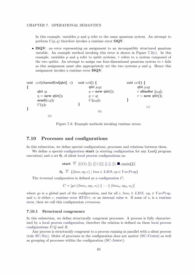
CHAPTER 7. OPERATIONAL SEMANTICS

In this example, variables p and q refer to the same quantum system. An attempt toperform U(p, q) therefore invokes a runtime error OQV.

• ISQV: an error representing an assignment to an incompatibly structured quantumvariable. An example method invoking this error is shown in Figure 7.3(c). In thisexample, variables p and q refer to qubit systems, r refers to a system composed ofthe two qubits. An attempt to assign one four-dimensional quantum system to r failsas this assignment must also appropriately set the two systems p and q. Hence thisassignment invokes a runtime error ISQV.

void ex1(channelEnd[qbit] c)

qbit q;q = new qbit();send(c,q);U(q);

(a)

void ex2() qbit p,q;q = new qbit();p = q;U(p,q);

(b)

void ex3() qbit p,q;r aliasfor [p,q];r = new q4it();

(c)

Figure 7.3: Example methods invoking runtime errors.

7.10 Processes and configurations

In this subsection, we define special configurations, processes and relations between them.We define a special configuration start (a starting configuration for any LanQ program

execution) and a set 0c of silent local process configurations as:

start def= [(((1), []), []) | (([], [], [], []),,main())]

0cdef= (lms, vp, ε) | lms ∈ LMS, vp ∈ V arProp

The terminal configuration is defined as a configuration C:

C = [gs | (lms1, vp1, v1) ‖ · · · ‖ (lmsn, vpn, vn)]

where gs is a global part of the configuration, and for all i, lmsi ∈ LMS, vpi ∈ V arProp,and vi is either ε, runtime error RTErr, or an internal value v. If some of vi is a runtimeerror, then we call this configuration erroneous.

7.10.1 Structural congruence

In this subsection, we define structurally congruent processes. A process is fully character-ized by a local process configuration, therefore the relation is defined on these local processconfigurations P,Q and R.

Any process is structurally congruent to a process running in parallel with a silent process(rule SC-Nil). Order of processes in the configuration does not matter (SC-Comm) as wellas grouping of processes within the configuration (SC-Assoc).

65

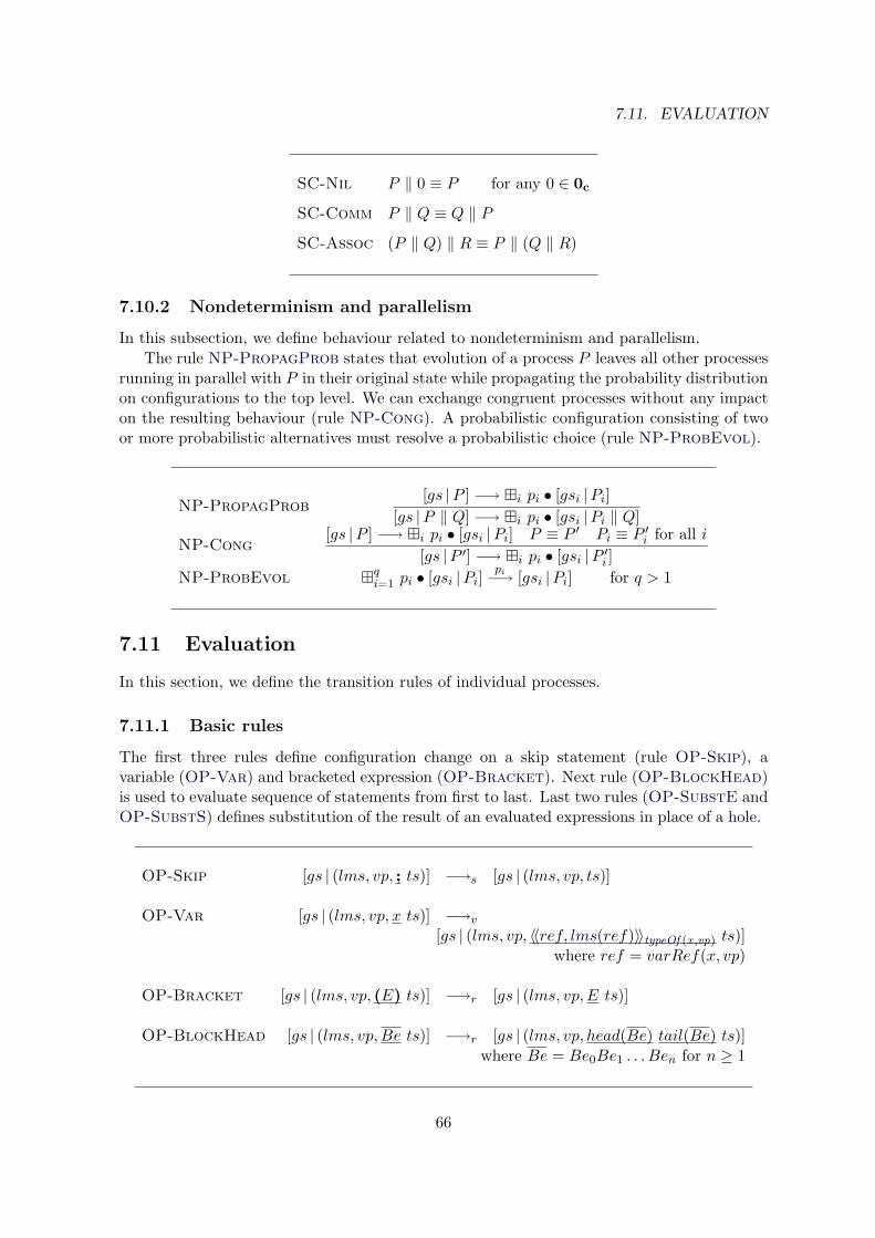
7.11. EVALUATION

SC-Nil P ‖ 0 ≡ P for any 0 ∈ 0c

SC-Comm P ‖ Q ≡ Q ‖ P

SC-Assoc (P ‖ Q) ‖ R ≡ P ‖ (Q ‖ R)

7.10.2 Nondeterminism and parallelism

In this subsection, we define behaviour related to nondeterminism and parallelism.The rule NP-PropagProb states that evolution of a process P leaves all other processes

running in parallel with P in their original state while propagating the probability distributionon configurations to the top level. We can exchange congruent processes without any impacton the resulting behaviour (rule NP-Cong). A probabilistic configuration consisting of twoor more probabilistic alternatives must resolve a probabilistic choice (rule NP-ProbEvol).

NP-PropagProb[gs |P ] −→ i pi • [gsi |Pi]

[gs |P ‖ Q] −→ i pi • [gsi |Pi ‖ Q]

NP-Cong[gs |P ] −→ i pi • [gsi |Pi] P ≡ P ′ Pi ≡ P ′

i for all i[gs |P ′] −→ i pi • [gsi |P ′

i ]NP-ProbEvol q

i=1 pi • [gsi |Pi]pi−→ [gsi |Pi] for q > 1

7.11 Evaluation

In this section, we define the transition rules of individual processes.

7.11.1 Basic rules

The first three rules define configuration change on a skip statement (rule OP-Skip), avariable (OP-Var) and bracketed expression (OP-Bracket). Next rule (OP-BlockHead)is used to evaluate sequence of statements from first to last. Last two rules (OP-SubstE andOP-SubstS) defines substitution of the result of an evaluated expressions in place of a hole.

OP-Skip [gs | (lms, vp, ; ts)] −→s [gs | (lms, vp, ts)]

OP-Var [gs | (lms, vp, x ts)] −→v

[gs | (lms, vp, 〈〈ref, lms(ref)〉〉typeOf (x ,vp) ts)]where ref = varRef(x, vp)

OP-Bracket [gs | (lms, vp, (E) ts)] −→r [gs | (lms, vp,E ts)]

OP-BlockHead [gs | (lms, vp,Be ts)] −→r [gs | (lms, vp, head(Be) tail(Be) ts)]where Be = Be0Be1 . . . Ben for n ≥ 1

66

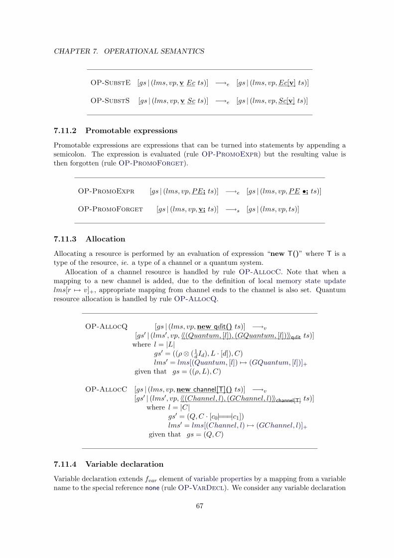
CHAPTER 7. OPERATIONAL SEMANTICS

OP-SubstE [gs | (lms, vp,v Ec ts)] −→e [gs | (lms, vp,Ec[v] ts)]

OP-SubstS [gs | (lms, vp,v Sc ts)] −→e [gs | (lms, vp, Sc[v] ts)]

7.11.2 Promotable expressions

Promotable expressions are expressions that can be turned into statements by appending asemicolon. The expression is evaluated (rule OP-PromoExpr) but the resulting value isthen forgotten (rule OP-PromoForget).

OP-PromoExpr [gs | (lms, vp, PE; ts)] −→e [gs | (lms, vp, PE •; ts)]

OP-PromoForget [gs | (lms, vp,v; ts)] −→s [gs | (lms, vp, ts)]

7.11.3 Allocation

Allocating a resource is performed by an evaluation of expression “new T()” where T is atype of the resource, ie. a type of a channel or a quantum system.

Allocation of a channel resource is handled by rule OP-AllocC. Note that when amapping to a new channel is added, due to the definition of local memory state updatelms[r 7→ v]+, appropriate mapping from channel ends to the channel is also set. Quantumresource allocation is handled by rule OP-AllocQ.

OP-AllocQ [gs | (lms, vp,new qdit() ts)] −→v

[gs′ | (lms′, vp, 〈〈(Quantum, [l]), (GQuantum, [l])〉〉qd it ts)]where l = |L|

gs′ = ((ρ⊗ (1dId), L · [d]), C)

lms′ = lms[(Quantum, [l]) 7→ (GQuantum, [l])]+given that gs = ((ρ, L), C)

OP-AllocC [gs | (lms, vp,new channel[T]() ts)] −→v

[gs′ | (lms′, vp, 〈〈(Channel, l), (GChannel, l)〉〉channel[T] ts)]where l = |C|

gs′ = (Q,C · [c0|== |=

c1])lms′ = lms[(Channel, l) 7→ (GChannel, l)]+

given that gs = (Q,C)

7.11.4 Variable declaration

Variable declaration extends fvar element of variable properties by a mapping from a variablename to the special reference none (rule OP-VarDecl). We consider any variable declaration

67

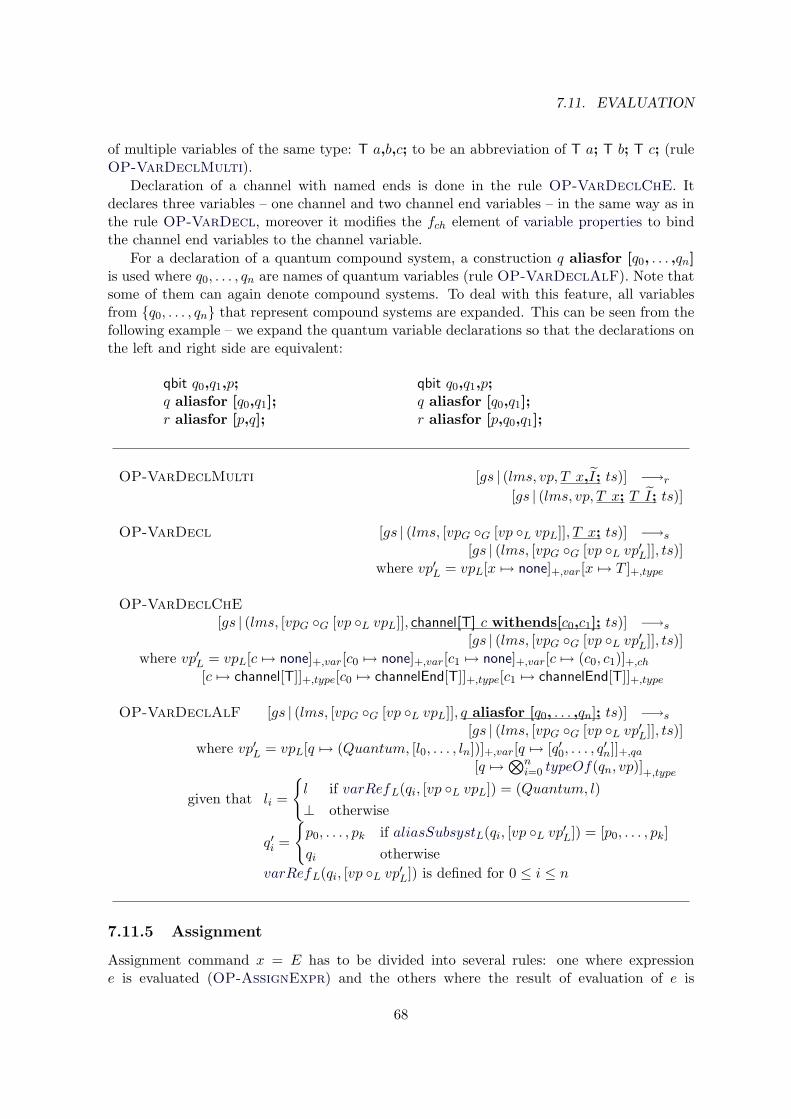
7.11. EVALUATION

of multiple variables of the same type: T a,b,c; to be an abbreviation of T a; T b; T c; (ruleOP-VarDeclMulti).

Declaration of a channel with named ends is done in the rule OP-VarDeclChE. Itdeclares three variables – one channel and two channel end variables – in the same way as inthe rule OP-VarDecl, moreover it modifies the fch element of variable properties to bindthe channel end variables to the channel variable.

For a declaration of a quantum compound system, a construction q aliasfor [q0, . . . ,qn]is used where q0, . . . , qn are names of quantum variables (rule OP-VarDeclAlF). Note thatsome of them can again denote compound systems. To deal with this feature, all variablesfrom q0, . . . , qn that represent compound systems are expanded. This can be seen from thefollowing example – we expand the quantum variable declarations so that the declarations onthe left and right side are equivalent:

qbit q0,q1,p;q aliasfor [q0,q1];r aliasfor [p,q];

qbit q0,q1,p;q aliasfor [q0,q1];r aliasfor [p,q0,q1];

OP-VarDeclMulti [gs | (lms, vp, T x,I; ts)] −→r

[gs | (lms, vp, T x; T I; ts)]

OP-VarDecl [gs | (lms, [vpG G [vp L vpL]], T x; ts)] −→s

[gs | (lms, [vpG G [vp L vp′L]], ts)]where vp′L = vpL[x 7→ none]+,var[x 7→ T ]+,type

OP-VarDeclChE[gs | (lms, [vpG G [vp L vpL]], channel[T] c withends[c0,c1]; ts)] −→s

[gs | (lms, [vpG G [vp L vp′L]], ts)]where vp′L = vpL[c 7→ none]+,var[c0 7→ none]+,var[c1 7→ none]+,var[c 7→ (c0, c1)]+,ch

[c 7→ channel[T]]+,type[c0 7→ channelEnd[T]]+,type[c1 7→ channelEnd[T]]+,type

OP-VarDeclAlF [gs | (lms, [vpG G [vp L vpL]], q aliasfor [q0, . . . ,qn]; ts)] −→s

[gs | (lms, [vpG G [vp L vp′L]], ts)]where vp′L = vpL[q 7→ (Quantum, [l0, . . . , ln])]+,var[q 7→ [q′0, . . . , q

′n]]+,qa

[q 7→⊗n

i=0 typeOf(qn, vp)]+,type

given that li =

l if varRefL(qi, [vp L vpL]) = (Quantum, l)⊥ otherwise

q′i =

p0, . . . , pk if aliasSubsystL(qi, [vp L vp′L]) = [p0, . . . , pk]qi otherwise

varRefL(qi, [vp L vp′L]) is defined for 0 ≤ i ≤ n

7.11.5 Assignment

Assignment command x = E has to be divided into several rules: one where expressione is evaluated (OP-AssignExpr) and the others where the result of evaluation of e is

68

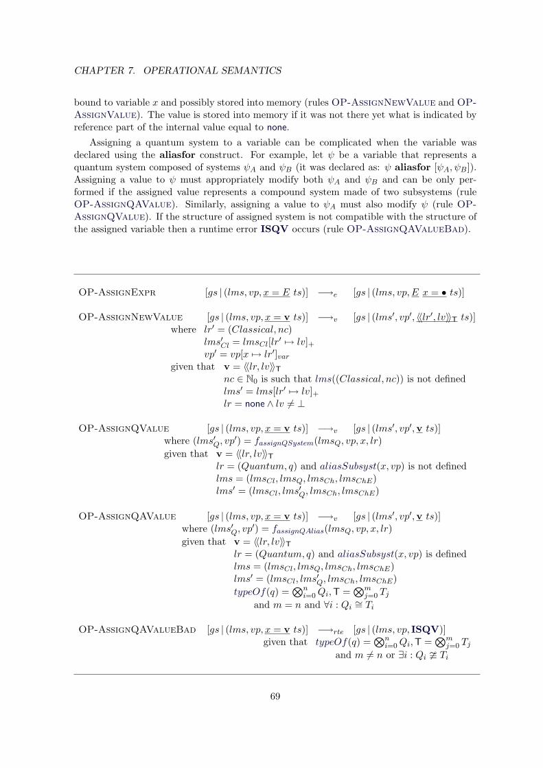
CHAPTER 7. OPERATIONAL SEMANTICS

bound to variable x and possibly stored into memory (rules OP-AssignNewValue and OP-AssignValue). The value is stored into memory if it was not there yet what is indicated byreference part of the internal value equal to none.

Assigning a quantum system to a variable can be complicated when the variable wasdeclared using the aliasfor construct. For example, let ψ be a variable that represents aquantum system composed of systems ψA and ψB (it was declared as: ψ aliasfor [ψA, ψB]).Assigning a value to ψ must appropriately modify both ψA and ψB and can be only per-formed if the assigned value represents a compound system made of two subsystems (ruleOP-AssignQAValue). Similarly, assigning a value to ψA must also modify ψ (rule OP-AssignQValue). If the structure of assigned system is not compatible with the structure ofthe assigned variable then a runtime error ISQV occurs (rule OP-AssignQAValueBad).

OP-AssignExpr [gs | (lms, vp, x = E ts)] −→e [gs | (lms, vp,E x = • ts)]

OP-AssignNewValue [gs | (lms, vp, x = v ts)] −→v [gs | (lms′, vp′, 〈〈lr′, lv〉〉T ts)]where lr′ = (Classical, nc)

lms′Cl = lmsCl[lr′ 7→ lv]+vp′ = vp[x 7→ lr′]var

given that v = 〈〈lr, lv〉〉Tnc ∈ N0 is such that lms((Classical, nc)) is not definedlms′ = lms[lr′ 7→ lv]+lr = none ∧ lv 6= ⊥

OP-AssignQValue [gs | (lms, vp, x = v ts)] −→v [gs | (lms′, vp′,v ts)]where (lms′Q, vp

′) = fassignQSystem(lmsQ, vp, x, lr)given that v = 〈〈lr, lv〉〉T

lr = (Quantum, q) and aliasSubsyst(x, vp) is not definedlms = (lmsCl, lmsQ, lmsCh, lmsChE)lms′ = (lmsCl, lms′Q, lmsCh, lmsChE)

OP-AssignQAValue [gs | (lms, vp, x = v ts)] −→v [gs | (lms′, vp′,v ts)]where (lms′Q, vp

′) = fassignQAlias(lmsQ, vp, x, lr)given that v = 〈〈lr, lv〉〉T

lr = (Quantum, q) and aliasSubsyst(x, vp) is definedlms = (lmsCl, lmsQ, lmsCh, lmsChE)lms′ = (lmsCl, lms′Q, lmsCh, lmsChE)typeOf(q) =

⊗ni=0Qi,T =

⊗mj=0 Tj

and m = n and ∀i : Qi ∼= Ti

OP-AssignQAValueBad [gs | (lms, vp, x = v ts)] −→rte [gs | (lms, vp, ISQV)]given that typeOf(q) =

⊗ni=0Qi,T =

⊗mj=0 Tj

and m 6= n or ∃i : Qi Ti

69

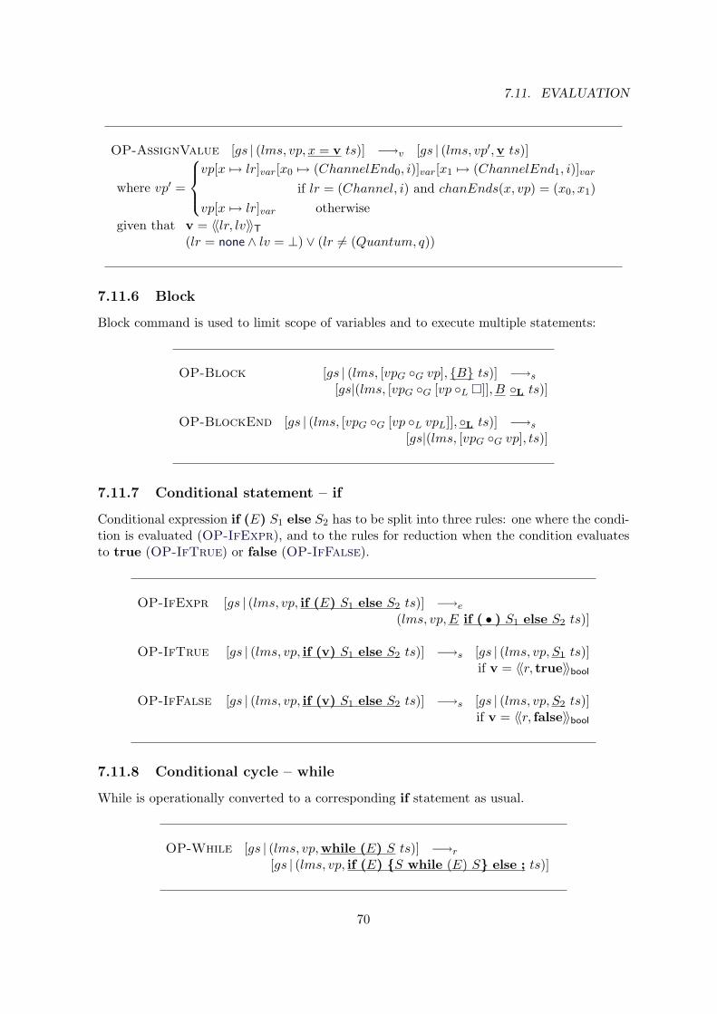
7.11. EVALUATION

OP-AssignValue [gs | (lms, vp, x = v ts)] −→v [gs | (lms, vp′,v ts)]

where vp′ =

vp[x 7→ lr]var[x0 7→ (ChannelEnd0, i)]var[x1 7→ (ChannelEnd1, i)]var

if lr = (Channel, i) and chanEnds(x, vp) = (x0, x1)vp[x 7→ lr]var otherwise

given that v = 〈〈lr, lv〉〉T(lr = none ∧ lv = ⊥) ∨ (lr 6= (Quantum, q))

7.11.6 Block

Block command is used to limit scope of variables and to execute multiple statements:

OP-Block [gs | (lms, [vpG G vp], B ts)] −→s

[gs|(lms, [vpG G [vp L ]], B L ts)]

OP-BlockEnd [gs | (lms, [vpG G [vp L vpL]], L ts)] −→s

[gs|(lms, [vpG G vp], ts)]

7.11.7 Conditional statement – if

Conditional expression if (E) S1 else S2 has to be split into three rules: one where the condi-tion is evaluated (OP-IfExpr), and to the rules for reduction when the condition evaluatesto true (OP-IfTrue) or false (OP-IfFalse).

OP-IfExpr [gs | (lms, vp, if (E) S1 else S2 ts)] −→e

(lms, vp,E if ( • ) S1 else S2 ts)]

OP-IfTrue [gs | (lms, vp, if (v) S1 else S2 ts)] −→s [gs | (lms, vp, S1 ts)]if v = 〈〈r, true〉〉bool

OP-IfFalse [gs | (lms, vp, if (v) S1 else S2 ts)] −→s [gs | (lms, vp, S2 ts)]if v = 〈〈r, false〉〉bool

7.11.8 Conditional cycle – while

While is operationally converted to a corresponding if statement as usual.

OP-While [gs | (lms, vp,while (E) S ts)] −→r

[gs | (lms, vp, if (E) S while (E) S else ; ts)]

70

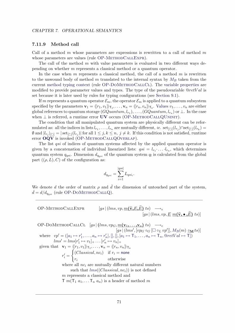
CHAPTER 7. OPERATIONAL SEMANTICS

7.11.9 Method call

Call of a method m whose parameters are expressions is rewritten to a call of method mwhose parameters are values (rule OP-MethodCallExpr).

The call of the method m with value parameters is evaluated in two different ways de-pending on whether m represents a classical method or a quantum operator.

In the case when m represents a classical method, the call of a method m is rewrittento the unwound body of method m translated to the internal syntax by MB taken from thecurrent method typing context (rule OP-DoMethodCallCl). The variable properties aremodified to provide parameter values and types. The type of the pseudovariable @retV al isset because it is later used by rules for typing configurations (see Section 9.1).

Ifm represents a quantum operator Em, the operator Em is applied to a quantum subsystemspecified by the parameters v1 = 〈〈r1, v1〉〉T1 , . . . ,vn = 〈〈rn, vn〉〉Tn . Values v1, . . . , vn are eitherglobal references to quantum storage (GQuantum, lr1), . . . , (GQuantum, lrn) or⊥. In the casewhen ⊥ is referred, a runtime error UV occurs (OP-MethodCallQUninit).

The condition that all manipulated quantum system are physically different can be refor-mulated as: all the indices in lists lr1 , . . . , lrn are mutually different, ie. set[](lrj )∩set[](lrk) =∅ and |lrj |[] = | set[](lrj )| for all 1 ≤ j, k ≤ n, j 6= k. If this condition is not satisfied, runtimeerror OQV is invoked (OP-MethodCallQOverlap).

The list qsi of indices of quantum systems affected by the applied quantum operator isgiven by a concatenation of individual linearized lists: qsi = lr1 · . . . ·lrn , which determinesquantum system qqsi. Dimension dqqsi of the quantum system ql is calculated from the globalpart ((ρ, L), C) of the configuration as:

dqqsi =|qsi|∑i=1

Lqsii .

We denote d the order of matrix ρ and d the dimension of untouched part of the system,d = d/dqqsi (rule OP-DoMethodCallQ).

OP-MethodCallExpr [gs | (lms, vp,m(v,E,E) ts) −→e

[gs | (lms, vp,E m(v, • ,E) ts)]

OP-DoMethodCallCl [gs | (lms, vpG,m(v1, . . . ,vn) ts) −→e

[gs | (lms′, [vpG G [ L vp′]],MB(m) M ts)]where vp′ = ([a1 7→ r′1, . . . , an 7→ r′n], [], [], [a1 7→ T1, . . . , an 7→ Tn,@retV al 7→ T])

lms′ = lms[r′1 7→ v1]+ . . . [r′n 7→ vn]+given that v1 = 〈〈r1, v1〉〉T1 , . . . ,vn = 〈〈rn, vn〉〉Tn

r′i =

(Classical, nci) if ri = none

ri otherwisewhere all nci are mutually different natural numbers

such that lms((Classical, nci)) is not definedm represents a classical method andT m(T1 a1, . . .Tn an) is a header of method m

71

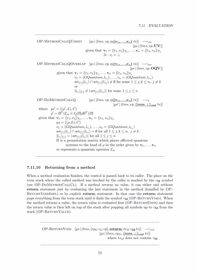
7.11. EVALUATION

OP-MethodCallQUninit [gs | (lms, vp,m(v1, . . . ,vn) ts)] −→rte

[gs | (lms, vp,UV)]given that v1 = 〈〈r1, v1〉〉T1 , . . . ,vn = 〈〈rn, vn〉〉Tn

∃i : vi = ⊥

OP-MethodCallQOverlap [gs | (lms, vp,m(v1, . . . ,vn) ts)] −→rte

[gs | (lms, vp,OQV)]given that v1 = 〈〈r1, v1〉〉T1 , . . . ,vn = 〈〈rn, vn〉〉Tn

v1 = (GQuantum, lr1), . . . , vn = (GQuantum, lrn)set[](lrj ) ∩ set[](lrk) 6= ∅ for some 1 ≤ j, k ≤ n, j 6= k

or|lrj |[] 6= | set[](lrj )| for some 1 ≤ j ≤ n

OP-DoMethodCallQ [gs | (lms, vp,m(v1, . . . ,vn) ts)] −→v

[gs′ | (lms, vp, 〈〈none,⊥〉〉void ts)]where gs′ = ((ρ′, L), C)

ρ′ = ΠT (Em ⊗ Id(ΠρΠT ))Πgiven that v1 = 〈〈r1, v1〉〉T1 , . . . ,vn = 〈〈rn, vn〉〉Tn

gs = ((ρ, L), C)v1 = (GQuantum, lr1), . . . , vn = (GQuantum, lrn)set[](lrj ) ∩ set[](lrk) = ∅ for all 1 ≤ j, k ≤ n, j 6= k

|lrj |[] = | set[](lrj )| for all 1 ≤ j ≤ nΠ is a permutation matrix which places affected quantum

systems to the head of ρ in the order given by v1, . . . ,vnm represents a quantum operator Em

7.11.10 Returning from a method

When a method evaluation finishes, the control is passed back to its caller. The place on theterm stack where the called method was invoked by the caller is marked by the M symbol(see OP-DoMethodCallCl). If a method returns no value, it can either end withoutreturn statement just by evaluating the last statement in the method (handled by OP-ReturnVoidImpl) or by explicit return; statement. In that case the return; statementpops everything from the term stack until it finds the symbol M (OP-ReturnVoid). Whenthe method returns a value, the return value is evaluated first (OP-ReturnExpr) and thenthe return value is then left on top of the stack after popping all symbols up to M from thestack (OP-ReturnValue).

OP-ReturnVoid [gs | (lms, [vpG G vp], return; tsM M ts)] −→ret

[gs | (lms, vpG, 〈〈none,⊥〉〉void ts)]where tsM does not contain M

72

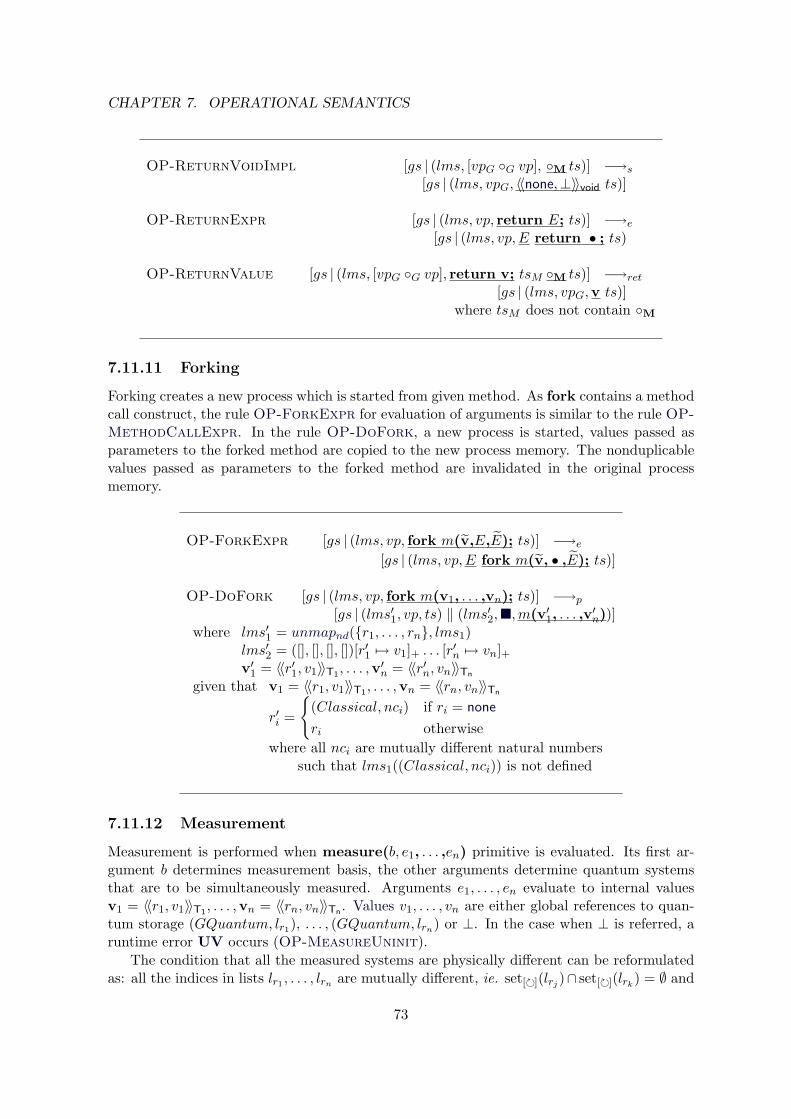
CHAPTER 7. OPERATIONAL SEMANTICS

OP-ReturnVoidImpl [gs | (lms, [vpG G vp], M ts)] −→s

[gs | (lms, vpG, 〈〈none,⊥〉〉void ts)]

OP-ReturnExpr [gs | (lms, vp, return E; ts)] −→e

[gs | (lms, vp,E return • ; ts)

OP-ReturnValue [gs | (lms, [vpG G vp], return v; tsM M ts)] −→ret

[gs | (lms, vpG,v ts)]where tsM does not contain M

7.11.11 Forking

Forking creates a new process which is started from given method. As fork contains a methodcall construct, the rule OP-ForkExpr for evaluation of arguments is similar to the rule OP-MethodCallExpr. In the rule OP-DoFork, a new process is started, values passed asparameters to the forked method are copied to the new process memory. The nonduplicablevalues passed as parameters to the forked method are invalidated in the original processmemory.

OP-ForkExpr [gs | (lms, vp, fork m(v,E,E); ts)] −→e

[gs | (lms, vp,E fork m(v, • ,E); ts)]

OP-DoFork [gs | (lms, vp, fork m(v1, . . . ,vn); ts)] −→p

[gs | (lms′1, vp, ts) ‖ (lms′2,,m(v′1, . . . ,v′n))]

where lms′1 = unmapnd(r1, . . . , rn, lms1)lms′2 = ([], [], [], [])[r′1 7→ v1]+ . . . [r′n 7→ vn]+v′1 = 〈〈r′1, v1〉〉T1 , . . . ,v

′n = 〈〈r′n, vn〉〉Tn

given that v1 = 〈〈r1, v1〉〉T1 , . . . ,vn = 〈〈rn, vn〉〉Tn

r′i =

(Classical, nci) if ri = none

ri otherwisewhere all nci are mutually different natural numbers

such that lms1((Classical, nci)) is not defined

7.11.12 Measurement

Measurement is performed when measure(b, e1, . . . ,en) primitive is evaluated. Its first ar-gument b determines measurement basis, the other arguments determine quantum systemsthat are to be simultaneously measured. Arguments e1, . . . , en evaluate to internal valuesv1 = 〈〈r1, v1〉〉T1 , . . . ,vn = 〈〈rn, vn〉〉Tn . Values v1, . . . , vn are either global references to quan-tum storage (GQuantum, lr1), . . . , (GQuantum, lrn) or ⊥. In the case when ⊥ is referred, aruntime error UV occurs (OP-MeasureUninit).

The condition that all the measured systems are physically different can be reformulatedas: all the indices in lists lr1 , . . . , lrn are mutually different, ie. set[](lrj )∩ set[](lrk) = ∅ and

73

7.11. EVALUATION

|lrj |[] = | set[](lrj )| for all 1 ≤ j, k ≤ n, j 6= k. If this condition is not satisfied, runtimeerror OQV is invoked (OP-MeasureOverlap).

The list qsi of indices of quantum systems to be measured is given by a concatenationof individual linearized lists: qsi = lr1 · . . . ·lrn , which determines quantum system qqsi. Di-mension dqqsi of the quantum system ql is calculated from the global part ((ρ, L), C) of theconfiguration as:

dqqsi =|qsi|∑i=1

Lqsii .

We denote d the order of matrix ρ and d the dimension of unmeasured part of the system,d = d/dqqsi .

In quantum mechanics, the possible results of the measurement are eigenvalues of theobservable. We assign to each eigenvalue an index in a list of all eigenvalues. This index isreturned as a result of evaluated measure expression. Indeed, it is possible that two or moreeigenvalues are the same (they are called degenerate eigenvalues). In this case, the obtainedresult is the first index of corresponding eigenvalue in the list. The list is indexed from zero.

Now we can formulate the rules for measurement:

OP-MeasureExpr [gs | (lms, vp,measure(v,E,E) ts] −→e

[gs | (lms, vp,E measure(v, • ,E) ts)]

OP-MeasureUninit [gs | (lms, vp,measure(vb,v1, . . . ,vn) ts)] −→rte

[gs | (lms, vp,UV)]given that v1 = 〈〈r1, v1〉〉T1 , . . . ,vn = 〈〈rn, vn〉〉Tn

∃i : vi = ⊥

OP-MeasureOverlap [gs | (lms, vp,measure(vb,v1, . . . ,vn) ts)] −→rte

[gs | (lms, vp,OQV)]given that v1 = 〈〈r1, v1〉〉T1 , . . . ,vn = 〈〈rn, vn〉〉Tn

v1 = (GQuantum, lr1), . . . , vn = (GQuantum, lrn)set[](lrj ) ∩ set[](lrk) 6= ∅ for some 1 ≤ j, k ≤ n, j 6= k

or|lrj |[] 6= | set[](lrj )| for some 1 ≤ j ≤ n

74

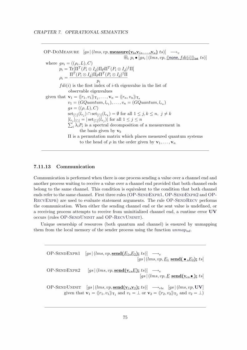
CHAPTER 7. OPERATIONAL SEMANTICS

OP-DoMeasure [gs | (lms, vp,measure(vb,v1, . . . ,vn) ts)] −→v

i pi • [gsi | (lms, vp, 〈〈none, fdi(i)〉〉int ts)]where gsi = ((ρi, L), C)

pi = Tr[ΠT (Pi ⊗ Id)ΠρΠT (Pi ⊗ Id)†Π]

ρi =ΠT (Pi ⊗ Id)ΠρΠT (Pi ⊗ Id)†Π

pifdi(i) is the first index of i-th eigenvalue in the list of

observable eigenvaluesgiven that v1 = 〈〈r1, v1〉〉T1 , . . . ,vn = 〈〈rn, vn〉〉Tn

v1 = (GQuantum, lr1), . . . , vn = (GQuantum, lrn)gs = ((ρ, L), C)set[](lrj ) ∩ set[](lrk) = ∅ for all 1 ≤ j, k ≤ n, j 6= k

|lrj |[] = | set[](lrj )| for all 1 ≤ j ≤ n∑i λiPi is a spectral decomposition of a measurement in

the basis given by vbΠ is a permutation matrix which places measured quantum systems

to the head of ρ in the order given by v1, . . . ,vn

7.11.13 Communication

Communication is performed when there is one process sending a value over a channel end andanother process waiting to receive a value over a channel end provided that both channel endsbelong to the same channel. This condition is equivalent to the condition that both channelends refer to the same channel. First three rules (OP-SendExpr1, OP-SendExpr2 and OP-RecvExpr) are used to evaluate statement arguments. The rule OP-SendRecv performsthe communication. When either the sending channel end or the sent value is undefined, ora receiving process attempts to receive from uninitialized channel end, a runtime error UVoccurs (rules OP-SendUninit and OP-RecvUninit).

Unique ownership of resources (both quantum and channel) is ensured by unmappingthem from the local memory of the sender process using the function unmapnd.

OP-SendExpr1 [gs | (lms, vp, send(E1,E2); ts)] −→e

[gs | (lms, vp,E1 send( • ,E2); ts]

OP-SendExpr2 [gs | (lms, vp, send(vc,E); ts)] −→e

[gs | (lms, vp,E send(vc, • ); ts]

OP-SendUninit [gs | (lms, vp, send(v1,v2); ts)] −→rte [gs | (lms, vp,UV]given that v1 = 〈〈r1, v1〉〉T1 and v1 = ⊥ or v2 = 〈〈r2, v2〉〉T2 and v2 = ⊥)

75

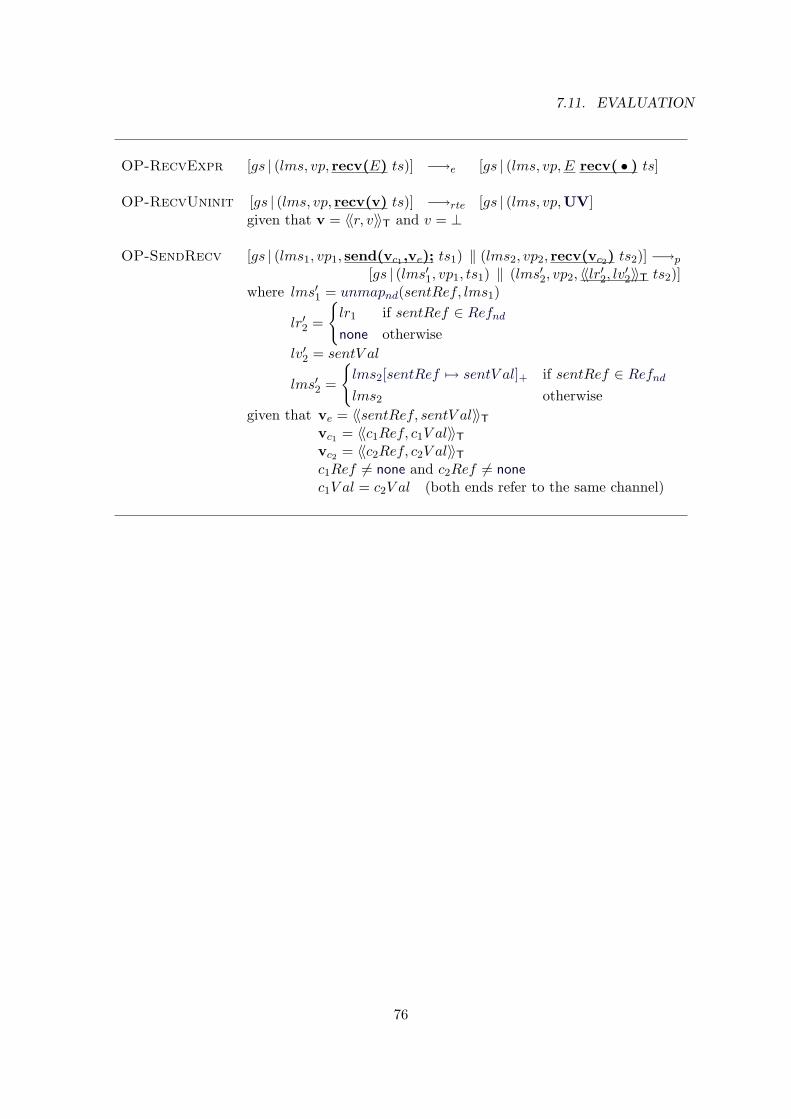
7.11. EVALUATION

OP-RecvExpr [gs | (lms, vp, recv(E) ts)] −→e [gs | (lms, vp,E recv( • ) ts]

OP-RecvUninit [gs | (lms, vp, recv(v) ts)] −→rte [gs | (lms, vp,UV]given that v = 〈〈r, v〉〉T and v = ⊥

OP-SendRecv [gs | (lms1, vp1, send(vc1,ve); ts1) ‖ (lms2, vp2, recv(vc2) ts2)] −→p

[gs | (lms′1, vp1, ts1) ‖ (lms′2, vp2, 〈〈lr′2, lv′2〉〉T ts2)]where lms′1 = unmapnd(sentRef, lms1)

lr′2 =

lr1 if sentRef ∈ Refndnone otherwise

lv′2 = sentV al

lms′2 =

lms2[sentRef 7→ sentV al]+ if sentRef ∈ Refndlms2 otherwise

given that ve = 〈〈sentRef, sentV al〉〉Tvc1 = 〈〈c1Ref, c1V al〉〉Tvc2 = 〈〈c2Ref, c2V al〉〉Tc1Ref 6= none and c2Ref 6= nonec1V al = c2V al (both ends refer to the same channel)

76

Chapter 8

Unique resource ownership

In this chapter, we prove that a resource, ie. a channel, a channel end, or a quantum system,is accessible to at most one process at a time.

Unique resource ownership is a natural requirement that must be fulfilled when we requesta deterministic evolution of individual processes running in a system. If two or more processeswere allowed to use the same resource at a time, we could get to the situation when they allwant to perform an exclusive operation on a resource. Then the order in which the operationswould be performed would be nondeterministic and could possibly lead to different results.

To ensure unique resource ownership, we must solve the issue here which a consequenceof the fact that variables referring to resources may refer both to an individual resource anda group of them.1 We must ensure that a resource, be it referred from a variable denoting agroup of resources or individual ones, gets inaccessible from a process when the control overthe resource is passed from this process to another one.

To solve this issue, we use the following idea: A group of resources is accessible from aprocess only if the process can access all of the resources which are elements of the group.

By accessibility of a quantum system to a process we mean that there is a mapping fromthe structured reference layer to the system memory layer. This mapping is stored in the localmemory state element lms in the local process configuration which describes the process state.This concept is formally defined for different kinds of resources in the following sections.

8.1 Unique quantum system ownership

In this section, we prove that a quantum system is always accessible by at most one process.

Definition 8.1.1. Let C = [gs | ls1 ‖ · · · ‖ lsn] be a configuration. Let us have a quantumsystem Q stored in the system memory at place referred by (GQuantum, [n]) ∈ RefG wheren ∈ N, and let Pi be a process described by the local process configuration lsi = (lms, vp, ts).We say that the quantum system Q is accessible to the process P iff there is a local referencel ∈ RefQ such that lms(l) = (GQuantum, p) where n ∈ set[](p).

Next we state what we mean by unique ownership of a quantum system. We formulate itas a property of a configuration.

1An example of a variable referring to a group of resources is an aliased quantum variable – it refers toseveral distinct quantum systems. Similarly, a channel variable can be seen as a group of two variables denotingindividual channel ends.

77

8.1. UNIQUE QUANTUM SYSTEM OWNERSHIP

Definition 8.1.2. Let C = [gs | ls1 ‖ · · · ‖ lsn] be a configuration. We say that C satisfiesunique quantum system ownership property if for any quantum system Q, there is at most oneprocess P described by the local process configuration lsi = (lms, vp, ts) for some i ∈ 1, . . . , nsuch that Q is accessible to P .

Lemma 8.1.3. The starting configuration start defined in Section 7.10 satisfies unique quan-tum system ownership property.

Proof. There is no resource stored in the system memory, therefore the lemma holds trivially.

Next we show that if a configuration which satisfies unique quantum system ownershipproperty is evolved by a transition, then the unique quantum system ownership propertyholds also for the new configuration.

Lemma 8.1.4. Let C0 be a configuration and C1 = qi=1pi • Ci,1 a mixed configuration such

that C0 −→ C1. If C0 satisfies unique quantum system ownership property then also Ci,1satisfies unique quantum system ownership property for all i.

Proof. This lemma trivially holds for all the transitions that only manipulate one process, ie.all the transition rules that form the relation −→ up to −→p. They do not change a localmemory state of any other process, hence if C0 satisfies unique quantum system ownershipproperty then also Ci,1 trivially satisfies unique quantum system ownership property for all i.

We must prove this lemma for the individual rules forming −→p, ie. for the rules OP-DoFork and OP-SendRecv:

OP-DoFork: By the definition of the rule OP-DoFork and by Lemma 7.5.2 we know thatthe quantum systems passed to the new process are not accessible to the original process.By the definition of the rule OP-DoFork, the quantum resources are accessible onlyto the new process. Therefore the configuration C1 satisfies unique quantum systemownership property,

OP-SendRecv: By the definition of the rule OP-SendRecv and by Lemma 7.5.2 we knowthat the quantum systems passed along the channel to the receiving process are notaccessible to the sending process in C1. By the definition of the rule OP-SendRecv,the quantum resources are accessible only to the receiving process. Therefore the con-figuration C1 satisfies unique quantum system ownership property.

Lemma 8.1.5. Let C0 = qi=1pi •Ci,0, q ≥ 1 be a mixed configuration and C1 be a configura-

tion such that C0pi−→ C1. If Ci,0 satisfies unique quantum system ownership property for all

i then also C1 satisfies unique quantum system ownership property.

Proof. Obvious from the definition of the rule NP-ProbEvol.

Theorem 8.1.6 (Unique quantum system ownership). For any configuration C such thatstart −→∗ C it holds that any quantum system stored in the system memory is accessible toat most one process.

Proof. Corollary of the Lemmata 8.1.3, 8.1.4 and 8.1.5.

78

CHAPTER 8. UNIQUE RESOURCE OWNERSHIP

8.2 Unique channel end ownership

In this section, we prove that a channel end is always accessible by at most one process.

Definition 8.2.1. Let Cnf = [gs | ls1 ‖ · · · ‖ lsn] be a configuration, gs = (Q,C). Let us havea channel D = D0|== |=D1 ∈ set(C) where D0, D1 denote ends of a channel, and let D be storedin the system memory at place referred by (GChannel, n) ∈ RefG where n ∈ N. Let Pi be aprocess described by the local process configuration lsi = (lms, vp, ts). We say that the channelend Di is accessible to the process P , i ∈ 0, 1, iff lms(ChannelEndi) = (GChannel, n).

Next we state what we mean by unique ownership of a channel end. We formulate it as aproperty of a configuration.

Definition 8.2.2. Let C = [gs | ls1 ‖ · · · ‖ lsn] be a configuration. We say that C satisfiesunique channel end ownership property if for any channel D = D0 |== |=

D1, there is atmost one process P0 described by the local process configuration lsi = (lms, vp, ts) for somei ∈ 1, . . . , n such that D0 is accessible to P0, and at most one process P1 described by thelocal process configuration lsj = (lms, vp, ts) for some j ∈ 1, . . . , n such that D1 is accessibleto P1.

Lemma 8.2.3. The starting configuration start defined in Section 7.10 satisfies unique chan-nel end ownership property.

Proof. There is no resource stored in the system memory, therefore the lemma holds trivially.

Next we show that if a configuration which satisfies unique channel end ownership propertyis evolved by some transition, then the unique channel end ownership property also holds inthe resulting configuration.

Lemma 8.2.4. Let C0 be a configuration and C1 = qi=1pi • Ci,1 a mixed configuration such

that C0 −→ C1. If C0 satisfies unique channel end ownership property then also Ci,1 satisfiesunique channel end ownership property for all i.

Proof. This lemma trivially holds for all the transitions that only manipulate one process,ie. all the transition rules that form the relation −→ up to −→p. They do not change alocal memory state of any other process, hence if C0 satisfies unique channel end ownershipproperty then also Ci,1 trivially satisfies unique channel end ownership property for all i.

We must prove this lemma for the individual rules forming −→p, ie. for the rules OP-DoFork and OP-SendRecv:

OP-DoFork: By the definition of the rule OP-DoFork, namely from the usage of localmemory state update function, we see that a channel end can be mapped into the newprocess local memory in two ways: either a channel end is directly passed from theoriginal process, or indirectly a channel end is passed as a part of its parent channel.

In both cases, the channel end is not accessible to the original process, being unmappedby the function unmapnd from the original process memory (see Lemmata 7.5.3 and7.5.4).

The channel end is hence accessible only to the new process, therefore the configurationC1 satisfies unique channel end ownership property,

79

8.3. UNIQUE CHANNEL OWNERSHIP

OP-SendRecv: Similarly, by the definition of the rule OP-SendRecv, namely from theusage of local memory state update function, we see that a channel end can be mappedinto the receiving process local memory in two ways: either a channel end is directlysent over a channel from the sending process, or a channel end is passed indirectly as apart of its parent channel. Clearly, the proof of this case is straightforward alterationof the case OP-DoFork.

Lemma 8.2.5. Let C0 = qi=1pi • Ci,0, q ≥ 1 be a mixed configuration and C1 be a configu-

ration such that C0pi−→ C1. If Ci,0 satisfies unique channel end ownership property for all i

then also C1 satisfies unique channel end ownership property.

Proof. Obvious from the definition of the rule NP-ProbEvol.

Theorem 8.2.6 (Unique channel end ownership). For any configuration C such thatstart −→∗ C it holds that any channel end of any channel stored in the system memoryis accessible to at most one process.

Proof. Corollary of the Lemmata 8.2.3, 8.2.4 and 8.2.5.

8.3 Unique channel ownership

In this section, we prove that a channel is always accessible by at most one process.

Definition 8.3.1. Let C = [gs | ls1 ‖ · · · ‖ lsn] be a configuration. Let us have a channelD, let D be stored in the system memory at place referred by (GChannel, n) ∈ RefG wheren ∈ N, and let Pi be a process described by the local process configuration lsi = (lms, vp, ts).We say that the channel D is accessible to the process P iff there is a local reference l ∈ RefChsuch that lms(l) = (GChannel, n).

Next we state what we mean by unique ownership of a channel. We formulate it as aproperty of a configuration.

Definition 8.3.2. Let C = [gs | ls1 ‖ · · · ‖ lsn] be a configuration. We say that C satisfiesunique channel ownership property if for any channel D, there is at most one process Pdescribed by the local process configuration lsi = (lms, vp, ts) for some i ∈ 1, . . . , n suchthat D is accessible to P .

Lemma 8.3.3. The starting configuration start defined in Section 7.10 satisfies unique chan-nel ownership property.

Proof. There is no resource stored in the system memory, therefore the lemma holds trivially.

Next we show that if a configuration which satisfies unique channel ownership propertyis evolved by a transition, then the unique channel ownership property holds also for theresulting configuration.

80

CHAPTER 8. UNIQUE RESOURCE OWNERSHIP

Lemma 8.3.4. Let C0 be a configuration and C1 = qi=1pi • Ci,1 a mixed configuration such

that C0 −→ C1. If C0 satisfies unique channel ownership property then also Ci,1 satisfiesunique channel ownership property for all i.

Proof. This lemma trivially holds for all the transitions that only manipulate one process, ie.all the transition rules that form the relation −→ up to −→p. They do not change a localmemory state of any other process, hence if C0 satisfies unique channel ownership propertythen also Ci,1 trivially satisfies unique channel ownership property for all i.

We must prove this lemma for the individual rules forming −→p, ie. for the rules OP-DoFork and OP-SendRecv:

OP-DoFork: By the definition of the rule OP-DoFork, namely from the usage of localmemory state update function, we see that a channel can be mapped into the newprocess local memory only when a channel is directly passed from the original process.

The channel is unmapped from the original process memory by the function unmapndif it is passed to the new process, but also in the case when one of its ends is passed tothe new process (see Lemmata 7.5.3 and 7.5.4).

Hence then number of processes to which the channel is accessible can only be decreased.Therefore the configuration C1 satisfies unique channel ownership property,

OP-SendRecv: By the definition of the rule OP-SendRecv, namely from the usage oflocal memory state update function, we know that a channel can be mapped into thereceiving process local memory only when a channel is directly passed along the channelfrom the sending process. Clearly, the proof of this case is straightforward alteration ofthe case OP-DoFork.

Lemma 8.3.5. Let C0 = qi=1pi • Ci,0, q ≥ 1 be a mixed configuration and C1 be a configu-

ration such that C0pi−→ C1. If Ci,0 satisfies unique channel ownership property for all i then

also C1 satisfies unique channel ownership property.

Proof. Obvious from the definition of the rule NP-ProbEvol.

Theorem 8.3.6 (Unique channel ownership). For any configuration C such thatstart −→∗ C it holds that any channel stored in the system memory is accessible to atmost one process.

Proof. Corollary of the Lemmata 8.3.3, 8.3.4 and 8.3.5.

Theorem 8.3.7 (Unique resource ownership). For any configuration C such thatstart −→∗ C it holds that any resource stored in the system memory is accessible to atmost one process.

Proof. Corollary of the Theorems 8.1.6, 8.2.6 and 8.3.6.

81

8.3. UNIQUE CHANNEL OWNERSHIP

82

Chapter 9

Type soundness

In this chapter, we prove type soundness (see eg. [Wright and Felleisen, 1994]) for LanQ.To prove type soundness theorem, we first define typing on configurations. Then in series

of progress lemmata proofs, we prove that any typable configuration can be reduced by somesemantic rule. After this proof, we prove series of type preservation lemmata stating that if aconfiguration gets reduced to another configuration, either a runtime error occurs or the typeof the configuration is preserved. These lemmata straightforwardly imply type soundness ofthe language.

However, we cannot prove the type soundness property for the unrestricted languagebecause it is possible that a program gets to a stuck configuration during the evaluation.This can happen because the send and recv constructs are blocking actions. Consider aprocess which attempts to send a value over a channel where no other process is receivingthe values from the other end of the channel. Then no semantic rule can be applied to thesending process. Symmetrically, it is indeed possible to define a process which attempts toreceive a value from a channel where no other process sends a value over this channel. Sucha process also cannot evolve, therefore the evaluation can get to a stuck configuration.

In other words, we can prove type soundness only for the noncommunicating part of thelanguage. Nevertheless, if to each send statement there is a corresponding recv expression,then it can be proved that the evaluation of a well-typed configuration never gets stuck, hencetype soundness could be proved for the unrestricted language.

9.1 Typing of configurations

To prove LanQ type soundness, we follow the approach of [Bierman, Parkinson, and Pitts,2003]. Before proving type preservation, we define typing of configurations in this subsectionin Figures 9.1 and 9.2.

Any configuration C = [gs | ls1 ‖ · · · ‖ lsn] is assigned a type T , written as C : T which isa cartesian product of types of local process configurations ls1, . . . , lsn. If the type of lsi isTi then T = (T1, . . . , Tn) (see the typing rule T-Config).

We call a configuration which can be assigned a type a well-typed configuration.The typing rules provide rules for well-formedness of configurations, hence also for local

process configurations. This indeed means that structure of variable properties and a termstack are tightly connected: To any block end mark L on the term stack, the variableproperties must contain a nonempty list of variable properties [vp L vpL] ∈ V arPropL (see

83

9.2. PROGRESS

rule TC-BlockEnd); to any method call mark M on the term stack, the variable propertiesmust contain a nonempty list of lists of variable properties [vpG G vp] ∈ V arProp (see rulesTC-RetHole, TC-RetExpr, TC-RetVoid and TC-RetImpl).

Typing of local process configurations as depicted in Figure 9.1 needs a deeper explanation.Contrary to usual typing of configurations known eg. from λ-calculi where one configurationcontains only one expression, we deal with the situation where there are many “expressions” inone configuration. These expressions are in our case term stack elements and they altogetherform a term stack of a local process configuration.

The type of a local process configuration is defined as σ → τ for types σ, τ . The type σspecifies the type of the hole in the top term stack element, τ specifies the type of the resultvalue. When there is no hole in the top term stack element, σ is void.

According to the configuration syntax, the top term stack element TE can contain atmost one hole. As the hole type σ is always known and the variable typing context can bededuced from variable properties, the type τ ′ of TE is derivable from the typing rules definedin Chapter 5.

If TE is the only term stack element in the local process configuration, its type determinesthe type of the result value τ . Otherwise, the type τ ′ is the type of a hole in the term stackelement right beneath TE and we can continue with typing the local process configurationwhere TE is popped from the term stack.

To derive variable typing context from local process configuration variable properties, wedefine a function vpContext. This function is defined as follows:

Definition 9.1.1. We define a function vpContext : V arProp→ (Names Types) whichcreates a variable typing context from variable properties as:

vpContext([L1 G K]) def= vpContextL(K)

vpContext() def= []

where vpContextL : V arPropL → (Names Types) is a function for getting a variabletyping context from local variable properties defined as:

vpContextL([K1 L (fvar, fch, fqa, ftype)])def= vpContextL(K1) ∗ ftype

vpContextL() def= []

9.2 Progress

In this section, we prove series of progress lemmata, ie. assertions claiming that any well-typed configuration which is not terminal can be reduced by some semantic rule. It alsofollows from the proof that the choice of the semantic rule for a single process is unique,hence the single process evolution is deterministic.

Lemma 9.2.1 (Progress Lemma for probabilism). Let C0 = qi=1pi • [gsi | lsi,0] be a mixed

configuration such that ` C0 : τ . Then there exists a configuration C1 such that C0p−→ C1.

Proof. Such a mixed configuration C0 is reduced by the rule NP-ProbEvol.

84

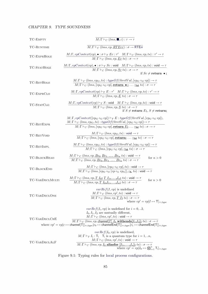
CHAPTER 9. TYPE SOUNDNESS

TC-Empty M ; Γ `C (lms,, ε) : τ → τ

TC-Runtime M ; Γ `C (lms, vp,RTErr) : σ → RTErr

TC-ExprHoleM ; Γ, vpContext(vp), • : σ `T Ec : τ ′ M ; Γ `C (lms, vp, ts) : τ ′ → τ

M ; Γ `C (lms, vp,Ec ts) : σ → τ

TC-StatHoleM ; Γ, vpContext(vp), • : σ `T Sc : void M ; Γ `C (lms, vp, ts) : void→ τ

M ; Γ `C (lms, vp, Sc ts) : σ → τif Sc 6= return • ;

TC-RetHoleM ; Γ `C (lms, vpG, ts) : typeOf(@retV al, [vpG G vp])→ τ

M ; Γ `C (lms, [vpG G vp], return • ; . . . M ts) : σ → τ

TC-ExprCloM ; Γ, vpContext(vp) `T E : τ ′ M ; Γ `C (lms, vp, ts) : τ ′ → τ

M ; Γ `C (lms, vp,E ts) : σ → τ

TC-StatCloM ; Γ, vpContext(vp) `T S : void M ; Γ `C (lms, vp, ts) : void→ τ

M ; Γ `C (lms, vp, S ts) : σ → τif S 6= return E;, S 6= return;

TC-RetExpr

M ; Γ, vpContext([vpG G vp]) `T E : typeOf(@retV al, [vpG G vp]),M ; Γ `C (lms, vpG, ts) : typeOf(@retV al, [vpG G vp])→ τ

M ; Γ `C (lms, [vpG G vp], return E; . . . M ts) : σ → τ

TC-RetVoidM ; Γ `C (lms, vpG, ts) : void→ τ

M ; Γ `C (lms, [vpG G vp], return; . . . M ts) : σ → τ

TC-RetImplM ; Γ `C (lms, vpG, ts) : typeOf(@retV al, [vpG G vp])→ τ

M ; Γ `C (lms, [vpG G vp], M ts) : σ → τ

TC-BlockHeadM ; Γ `C (lms, vp,Be0 Be1 . . . Ben ts) : void→ τ

M ; Γ `C (lms, vp,Be0 Be1 . . . Ben ts) : σ → τfor n > 0

TC-BlockEndM ; Γ `C (lms, [vpG G vp], ts) : void→ τ

M ; Γ `C (lms, [vpG G [vp L vpL]], L ts) : void→ τ

TC-VarDeclMultiM ; Γ `C (lms, vp, T I0; T I1, . . . ,In; ts) : void→ τ

M ; Γ `C (lms, vp, T I0,I1, . . . ,In; ts) : σ → τfor n > 0

TC-VarDeclOne

varRef(I, vp) is undefinedM ; Γ `C (lms, vp′, ts) : void→ τ

M ; Γ `C (lms, vp, T I; ts) : σ → τwhere vp′ = vp[I 7→ T]+,type

TC-VarDeclChE

varRef(Ii, vp) is undefined for i = 0, ..2,I0, I1, I2 are mutually different,M ; Γ `C (lms, vp′, ts) : void→ τ

M ; Γ `C (lms, vp, channel[T ] I0 withends[I1,I2]; ts) : σ → τwhere vp′ = vp[c 7→ channel[T]]+,type[c0 7→ channelEnd[T]]+,type[c1 7→ channelEnd[T]]+,type

TC-VarDeclAlF

varRef(I0, vp) is undefined,M ; Γ `T Ii : Ti Ti is a quantum type for i = 1, ..n,

M ; Γ `C (lms, vp′, ts) : void→ τ

M ; Γ `C (lms, vp, I0 aliasfor [I1, . . . ,In]; ts) : σ → τwhere vp′ = vp[I0 7→

⊗ni=1 Ti]+,type

Figure 9.1: Typing rules for local process configurations.

85

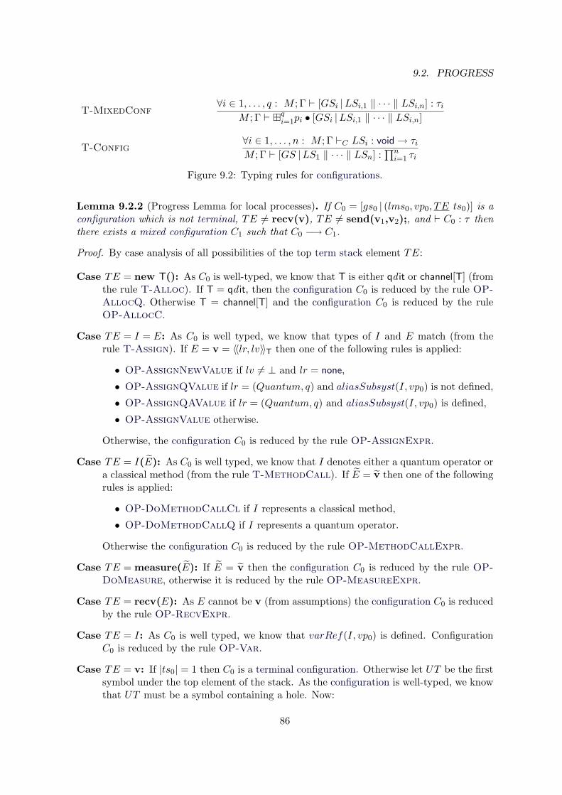
9.2. PROGRESS

T-MixedConf∀i ∈ 1, . . . , q : M ; Γ ` [GSi |LSi,1 ‖ · · · ‖ LSi,n] : τi

M ; Γ ` qi=1pi • [GSi |LSi,1 ‖ · · · ‖ LSi,n]

T-Config∀i ∈ 1, . . . , n : M ; Γ `C LSi : void→ τiM ; Γ ` [GS |LS1 ‖ · · · ‖ LSn] :

∏ni=1 τi

Figure 9.2: Typing rules for configurations.

Lemma 9.2.2 (Progress Lemma for local processes). If C0 = [gs0 | (lms0, vp0, TE ts0)] is aconfiguration which is not terminal, TE 6= recv(v), TE 6= send(v1,v2);, and ` C0 : τ thenthere exists a mixed configuration C1 such that C0 −→ C1.

Proof. By case analysis of all possibilities of the top term stack element TE:

Case TE = new T(): As C0 is well-typed, we know that T is either qd it or channel[T] (fromthe rule T-Alloc). If T = qd it, then the configuration C0 is reduced by the rule OP-AllocQ. Otherwise T = channel[T] and the configuration C0 is reduced by the ruleOP-AllocC.

Case TE = I = E: As C0 is well typed, we know that types of I and E match (from therule T-Assign). If E = v = 〈〈lr, lv〉〉T then one of the following rules is applied:

• OP-AssignNewValue if lv 6= ⊥ and lr = none,

• OP-AssignQValue if lr = (Quantum, q) and aliasSubsyst(I, vp0) is not defined,

• OP-AssignQAValue if lr = (Quantum, q) and aliasSubsyst(I, vp0) is defined,

• OP-AssignValue otherwise.

Otherwise, the configuration C0 is reduced by the rule OP-AssignExpr.

Case TE = I(E): As C0 is well typed, we know that I denotes either a quantum operator ora classical method (from the rule T-MethodCall). If E = v then one of the followingrules is applied:

• OP-DoMethodCallCl if I represents a classical method,

• OP-DoMethodCallQ if I represents a quantum operator.

Otherwise the configuration C0 is reduced by the rule OP-MethodCallExpr.

Case TE = measure(E): If E = v then the configuration C0 is reduced by the rule OP-DoMeasure, otherwise it is reduced by the rule OP-MeasureExpr.

Case TE = recv(E): As E cannot be v (from assumptions) the configuration C0 is reducedby the rule OP-RecvExpr.

Case TE = I: As C0 is well typed, we know that varRef(I, vp0) is defined. ConfigurationC0 is reduced by the rule OP-Var.

Case TE = v: If |ts0| = 1 then C0 is a terminal configuration. Otherwise let UT be the firstsymbol under the top element of the stack. As the configuration is well-typed, we knowthat UT must be a symbol containing a hole. Now:

86

CHAPTER 9. TYPE SOUNDNESS

Case UT = Ec: Configuration C0 is reduced by the rule OP-SubstE.

Case UT = Sc: Configuration C0 is reduced by the rule OP-SubstS.

Case TE = (E): Configuration C0 is reduced by the rule OP-Bracket.

Case TE = T I;: If TE = T I; then the configuration C0 is reduced by the rule OP-VarDecl. Otherwise it is reduced by the rule OP-VarDeclMulti.

Case TE = channel[T] I withends[I,I];: Configuration C0 is reduced by the rule OP-Var-DeclChE.

Case TE = q aliasfor [q0, . . . ,qn];: Configuration C0 is reduced by the rule OP-VarDecl-AlF.

Case TE = ;: Configuration C0 is reduced by the rule OP-Skip.

Case TE = PE;: If PE = v then the configuration C0 is reduced by the rule OP-Promo-Forget, otherwise it is reduced by OP-PromoExpr.

Case TE = L: Configuration C0 is reduced by the rule OP-BlockEnd.

Case TE = Be: Configuration C0 is reduced by the rule OP-BlockHead.

Case TE = B: Configuration C0 is reduced by the rule OP-Block.

Case TE = if (E) S1 else S2: If E = v, then the configuration is reduced by the rule OP-IfTrue (OP-IfFalse) when v is true (false). Otherwise, the configuration C0 isreduced by the rule OP-IfExpr.

Case TE = while (E) S: Configuration C0 is reduced by the rule OP-While.

Case TE = M: Configuration C0 is reduced by the rule OP-ReturnVoidImpl.

Case TE = return;: Configuration C0 is reduced by the rule OP-ReturnVoid.

Case TE = return E;: If E = v then the configuration C0 is reduced by the rule OP-ReturnValue, otherwise it is reduced by OP-ReturnExpr.

Case TE = fork m(E);: If E = v then the configuration C0 is reduced by the rule OP-DoFork. Otherwise it is reduced by the rule OP-ForkExpr.

Case TE = send(E1,E2);: If E1 6= v then the configuration C0 is reduced by the rule OP-SendExpr1. If E2 6= v, the configuration C0 is reduced by the rule OP-SendExpr2.Case E1 = v1 and E2 = v2 is prohibited by the assumptions.

Lemma 9.2.3 (Progress Lemma for communication). Let C0 = [gs0 | (lms0, vp0, recv(v) ts0) ‖(lms1, vp1, send(v1,v2); ts1) ‖ ls2 ‖ · · · ‖ lsn] : τ be a well-typed configuration. Then thereexists a configuration C1 such that C0 −→ C1.

Proof. Such a configuration is not terminal because of the elements recv(v) and send(v1,v2);on tops of the process term stacks. It is reduced by the rule OP-SendRecv.

87

9.3. TYPE PRESERVATION

Corollary 9.2.4. It is possible that a process evolves to a stuck configuration. This is thecase when one process attempts to send/receive a value over a channel end and there is nomatching process receiving/sending over the corresponding channel end.

9.3 Type preservation

9.3.1 Evaluation theorems

In the definition of LanQ semantics, we assumed that an expression always evaluates to avalue (or diverges or gets stuck due to incorrect send/recv pairing, or invokes a runtimeerror). This assumption was used in all rules which manipulate a subexpression Sub of astatement or an expression: The subexpression Sub is pushed onto the top of the term stackand the place of the awaited result in the original statement/expression is marked with a hole• (see eg. the rule OP-AssignExpr). We expect that if the evaluation correctly finishes, thesubexpression evaluates to an internal value that in a subsequent step replaces the hole.

However, we have not yet shown that the subexpression evaluation accomplishes this asser-tion. We have to prove that the statement/expression awaiting the result of the subexpressionevaluation is not modified before the evaluation of the subexpression yields an internal value(unless a runtime error occurs).

This will be shown in this subsection. We will use the following semantic predicates onconfigurations:

• ExpOk which is defined for configurations where the top term stack element of the firstlocal process configuration is some expression E, and

• BFOk and StkRetOk which is defined for configurations where the top term stackelement of the first local process configuration is some block-forming statement B.

Satisfiability of these predicates is determined by the future evolution of the configurationsin question.

The defined predicates are then used in the proof of the statement that if the syntacticpredicate RetOk defined in Chapter 5.1 is satisfied for a block-forming statement B then anycontrol path of evaluation of B reaches a return; or return E; statement, or a runtime error,or diverges, or gets stuck due to incorrect send/recv pairing (see Lemma 9.3.10). This proofis later used in proving type preservation lemma for −→s (see Lemma 9.3.16, proof of thecase OP-ReturnVoidImpl).

Definition 9.3.1. For an expression E, we define a predicate ExpOk(E): ExpOk(E) issatisfied iff for any configuration C0 = [gs0 | (lms0, vp0, E ts0)] : τ , the evaluation of C0 eitherdiverges or gets stuck due to incorrect send/recv pairing, or reaches one of the followingconfigurations:

• [gsn | (lms0,n, vp0,n,v ts0) ‖ · · · ‖ (lmsk,n, vpk,n, tsk,n)], k ≥ 0, or

• [gsn | (lms0,n, vp0,n, RTErr) ‖ · · · ‖ (lmsk,n, vpk,n, tsk,n)], k ≥ 0.

Definition 9.3.2. For a block-forming statement B, we define a predicate BFOk(B):BFOk(B) is satisfied iff for any configuration C0 = [gs0 | (lms0, vp0, B ts0)] : τ , the eval-uation either diverges or gets stuck due to incorrect send/recv pairing, or reaches one of thefollowing configurations:

88

CHAPTER 9. TYPE SOUNDNESS

• [gsn | (lms0,n, vp0,n, ts0) ‖ · · · ‖ (lmsk,n, vpk,n, tsk,n)], k ≥ 0, or

• [gsn | (lms0,n, vp0,n, return; ts0,n ts0) ‖ · · · ‖ (lmsk,n, vpk,n, tsk,n)], k ≥ 0, ts0,n does notcontain M, or

• [gsn | (lms0,n, vp0,n, return v; ts0,n ts0) ‖ · · · ‖ (lmsk,n, vpk,n, tsk,n)], k ≥ 0, ts0,n doesnot contain M, or

• [gsn | (lms0,n, vp0,n, RTErr) ‖ · · · ‖ (lmsk,n, vpk,n, tsk,n)], k ≥ 0.

We further define a predicate StkRetOk(B): StkRetOk(E) is satisfied iff for any well-typed configuration C0 = [gs0 | (lms0, vp0, B M ts0)] : τ , the evaluation either diverges orgets stuck due to incorrect send/recv pairing, or reaches one of the following configurations:

• [gsn | (lms0,n, vp0,n,v ts0) ‖ · · · ‖ (lmsk,n, vpk,n, tsk,n)], k ≥ 0, or

• [gsn | (lms0,n, vp0,n, RTErr) ‖ · · · ‖ (lmsk,n, vpk,n, tsk,n)], k ≥ 0.

Lemma 9.3.3. Let B be a block-forming statement such that BFOk(B). Then StkRetOk(B).

Proof. The evaluation starts from the following configuration:

[gs0 | (lms0, vp0, B M ts0)]

From BFOk(B) we know that evolution of this configuration:

• Diverges or gets stuck due to incorrect send/recv pairing, or gets to a configuration:

[gsn | (lmsn, vpn, RTErr) ‖ · · · ‖ (lmsk,n, vpk,n, tsk,n)]

therefore the lemma holds.

• Gets to a configuration:

[gsn′ | (lmsn′ , vpn′ , return; tsn′ M ts0) ‖ · · · ‖ (lmsk,n′ , vpk,n′ , tsk,n′)]

By application of OP-ReturnVoid, the 0-th process gets to a configuration:

[gsn′ | (lmsn′ , vpn′ , 〈〈none,⊥〉〉void ts0) ‖ · · · ‖ (lmsk,n′ , vpk,n′ , tsk,n′)]

therefore the lemma holds.

• Gets to a configuration:

[gsn′ | (lmsn′ , vpn′ , return v; tsn′ M ts0) ‖ · · · ‖ (lmsk,n′ , vpk,n′ , tsk,n′)]

By application of OP-ReturnValue, the 0-th process gets to a configuration:

[gsn′ | (lmsn′ , vpn′ ,v ts0) ‖ · · · ‖ (lmsk,n′ , vpk,n′ , tsk,n′)]

therefore the lemma holds.

89

9.3. TYPE PRESERVATION

We want to prove that for any expression E, the predicate ExpOk(E) is satisfied. Wedo this by defining inductive syntactic predicates ExpOki and BFOki with respect to thestructure of E and B, respectively. The dependency is the following (a ← b means a isdependent on b):

ExpOk0 BFOk0oo ExpOk1

oo . . .oo ExpOkioo BFOkioo · · ·oo

Definition 9.3.4. Let E be an expression, B be a block-forming statement. We define pred-icates ExpOk0(E) and BFOk0(B) :

ExpOk0(E) ⇐⇒ E does not contain I(E) as its subexpression.BFOk0(B) ⇐⇒ B contains only such subexpressions E which satisfy ExpOk0(E).

For any i ∈ N0, we further define predicates ExpOki+1(E) and BFOki+1(B) :

ExpOki+1(E) ⇐⇒ For any subexpression E0 of E, ExpOki(E0) is satisfiedor E0 = I(E) and BFOki(MB(I)) is satisfied.

BFOki+1(B) ⇐⇒ B contains only such subexpressions E which satisfy ExpOki+1(E).

Next we show the connection between the syntactic predicates ExpOki(E) (BFOki(E))and their semantic counterparts ExpOk (BFOk).

Lemma 9.3.5. Let E be an expression such that ExpOk0(E). Then ExpOk(E) is satisfied.

Proof. By induction on the structure of E. Let C0 = [gs0 | (lms0, vp0, E ts0)] : τ be anyconfiguration. Base case:

Case E = v: ExpOk(v) trivially.

Case E = I: By application of OP-Var we reach configuration [gs | (lms, vp,v ts0)], henceExpOk(E).

Case E = new T(): By application of OP-AllocC/OP-AllocQ reaches configuration[gs | (lms, vp,v ts0)], hence ExpOk(E).

Case E = I = v: By application of OP-AssignNewValue/OP-AssignQAValue/OP-AssignQValue/OP-AssignValue we reach configuration [gs | (lms, vp,v ts0)],hence ExpOk(E); by application of OP-AssignQAValueBad we reach configuration[gs | (lms, vp, ISQV)], hence ExpOk(E).

Case E = recv(v): By application of OP-SendRecv we reach configuration[gs | (lms, vp,v ts0)], hence ExpOk(E); by application of OP-RecvUninit we reachconfiguration [gs | (lms, vp,UV)], hence ExpOk(E). If there is no corresponding sendstatement, the configuration gets stuck due to incorrect send/recv pairing.

Case E = measure(v): By subsequent application of rules OP-DoMeasure andNP-ProbEvol we reach configuration [gs | (lms, vp,v ts0)], hence ExpOk(E); by ap-plication of OP-MeasureUninit we reach configuration [gs | (lms, vp,UV)], henceExpOk(E); by application of OP-MeasureOverlap we reach configuration[gs | (lms, vp,OQV)], hence ExpOk(E).

90

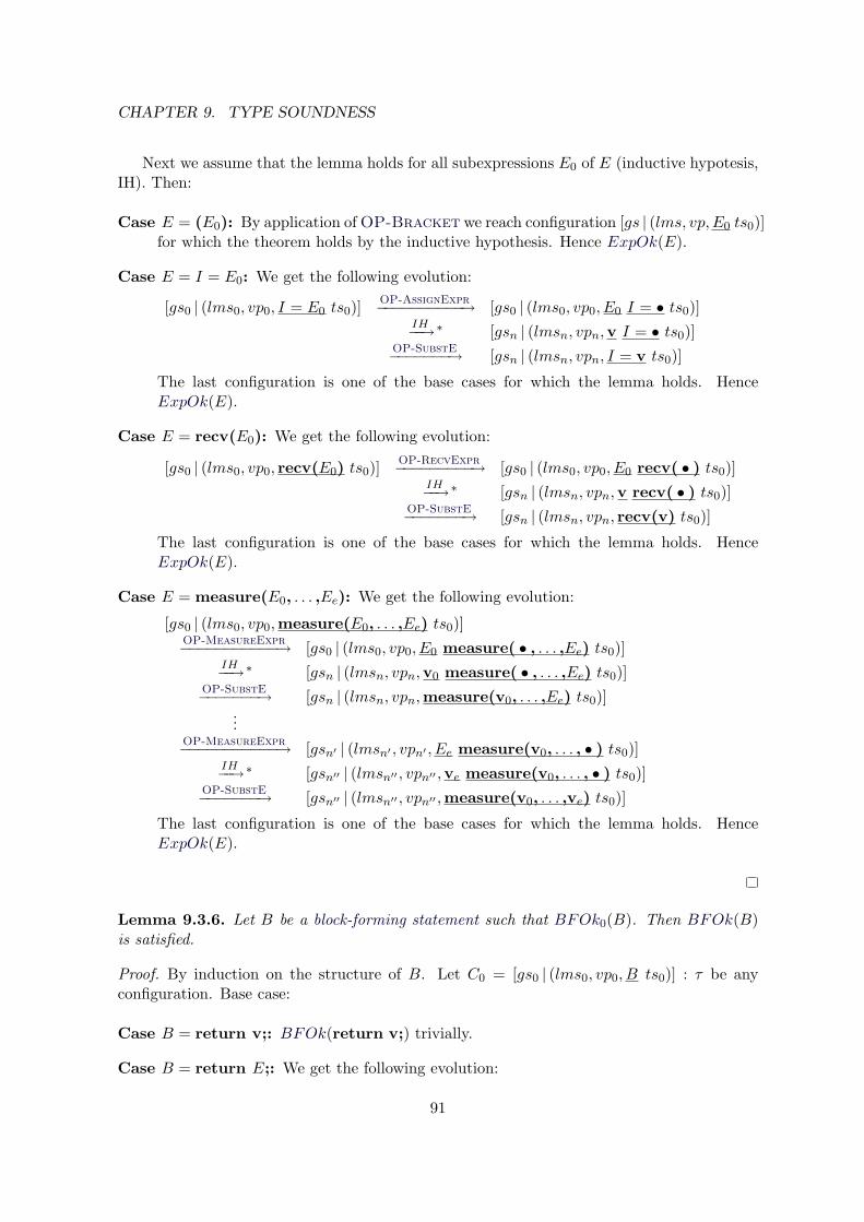
CHAPTER 9. TYPE SOUNDNESS

Next we assume that the lemma holds for all subexpressions E0 of E (inductive hypotesis,IH). Then:

Case E = (E0): By application of OP-Bracket we reach configuration [gs | (lms, vp,E0 ts0)]for which the theorem holds by the inductive hypothesis. Hence ExpOk(E).

Case E = I = E0: We get the following evolution:

[gs0 | (lms0, vp0, I = E0 ts0)]OP-AssignExpr−−−−−−−−−−→ [gs0 | (lms0, vp0, E0 I = • ts0)]

IH−−→∗ [gsn | (lmsn, vpn,v I = • ts0)]OP-SubstE−−−−−−−→ [gsn | (lmsn, vpn, I = v ts0)]

The last configuration is one of the base cases for which the lemma holds. HenceExpOk(E).

Case E = recv(E0): We get the following evolution:

[gs0 | (lms0, vp0, recv(E0) ts0)]OP-RecvExpr−−−−−−−−−→ [gs0 | (lms0, vp0, E0 recv( • ) ts0)]

IH−−→∗ [gsn | (lmsn, vpn,v recv( • ) ts0)]OP-SubstE−−−−−−−→ [gsn | (lmsn, vpn, recv(v) ts0)]

The last configuration is one of the base cases for which the lemma holds. HenceExpOk(E).

Case E = measure(E0, . . . ,Ee): We get the following evolution:

[gs0 | (lms0, vp0,measure(E0, . . . ,Ee) ts0)]OP-MeasureExpr−−−−−−−−−−−→ [gs0 | (lms0, vp0, E0 measure( • , . . . ,Ee) ts0)]

IH−−→∗ [gsn | (lmsn, vpn,v0 measure( • , . . . ,Ee) ts0)]OP-SubstE−−−−−−−→ [gsn | (lmsn, vpn,measure(v0, . . . ,Ee) ts0)]

...OP-MeasureExpr−−−−−−−−−−−→ [gsn′ | (lmsn′ , vpn′ , Ee measure(v0, . . . , • ) ts0)]

IH−−→∗ [gsn′′ | (lmsn′′ , vpn′′ ,ve measure(v0, . . . , • ) ts0)]OP-SubstE−−−−−−−→ [gsn′′ | (lmsn′′ , vpn′′ ,measure(v0, . . . ,ve) ts0)]

The last configuration is one of the base cases for which the lemma holds. HenceExpOk(E).

Lemma 9.3.6. Let B be a block-forming statement such that BFOk0(B). Then BFOk(B)is satisfied.

Proof. By induction on the structure of B. Let C0 = [gs0 | (lms0, vp0, B ts0)] : τ be anyconfiguration. Base case:

Case B = return v;: BFOk(return v;) trivially.

Case B = return E;: We get the following evolution:

91

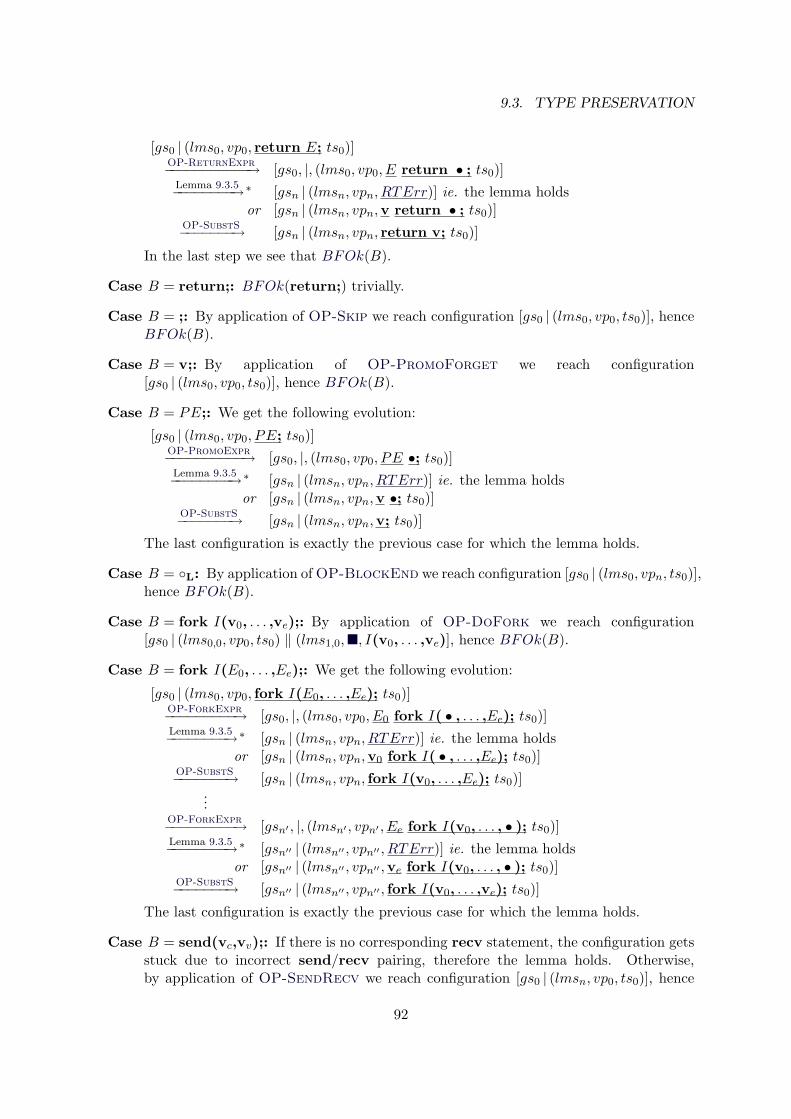
9.3. TYPE PRESERVATION

[gs0 | (lms0, vp0, return E; ts0)]OP-ReturnExpr−−−−−−−−−−−→ [gs0, |, (lms0, vp0, E return • ; ts0)]

Lemma 9.3.5−−−−−−−−→∗ [gsn | (lmsn, vpn, RTErr)] ie. the lemma holdsor [gsn | (lmsn, vpn,v return • ; ts0)]

OP-SubstS−−−−−−−→ [gsn | (lmsn, vpn, return v; ts0)]

In the last step we see that BFOk(B).

Case B = return;: BFOk(return;) trivially.

Case B = ;: By application of OP-Skip we reach configuration [gs0 | (lms0, vp0, ts0)], henceBFOk(B).

Case B = v;: By application of OP-PromoForget we reach configuration[gs0 | (lms0, vp0, ts0)], hence BFOk(B).

Case B = PE;: We get the following evolution:

[gs0 | (lms0, vp0, PE; ts0)]OP-PromoExpr−−−−−−−−−−→ [gs0, |, (lms0, vp0, PE •; ts0)]Lemma 9.3.5−−−−−−−−→∗ [gsn | (lmsn, vpn, RTErr)] ie. the lemma holds

or [gsn | (lmsn, vpn,v •; ts0)]OP-SubstS−−−−−−−→ [gsn | (lmsn, vpn,v; ts0)]

The last configuration is exactly the previous case for which the lemma holds.

Case B = L: By application of OP-BlockEnd we reach configuration [gs0 | (lms0, vpn, ts0)],hence BFOk(B).

Case B = fork I(v0, . . . ,ve);: By application of OP-DoFork we reach configuration[gs0 | (lms0,0, vp0, ts0) ‖ (lms1,0,, I(v0, . . . ,ve)], hence BFOk(B).

Case B = fork I(E0, . . . ,Ee);: We get the following evolution:

[gs0 | (lms0, vp0, fork I(E0, . . . ,Ee); ts0)]OP-ForkExpr−−−−−−−−−→ [gs0, |, (lms0, vp0, E0 fork I( • , . . . ,Ee); ts0)]Lemma 9.3.5−−−−−−−−→∗ [gsn | (lmsn, vpn, RTErr)] ie. the lemma holds

or [gsn | (lmsn, vpn,v0 fork I( • , . . . ,Ee); ts0)]OP-SubstS−−−−−−−→ [gsn | (lmsn, vpn, fork I(v0, . . . ,Ee); ts0)]

...OP-ForkExpr−−−−−−−−−→ [gsn′ , |, (lmsn′ , vpn′ , Ee fork I(v0, . . . , • ); ts0)]Lemma 9.3.5−−−−−−−−→∗ [gsn′′ | (lmsn′′ , vpn′′ , RTErr)] ie. the lemma holds

or [gsn′′ | (lmsn′′ , vpn′′ ,ve fork I(v0, . . . , • ); ts0)]OP-SubstS−−−−−−−→ [gsn′′ | (lmsn′′ , vpn′′ , fork I(v0, . . . ,ve); ts0)]

The last configuration is exactly the previous case for which the lemma holds.

Case B = send(vc,vv);: If there is no corresponding recv statement, the configuration getsstuck due to incorrect send/recv pairing, therefore the lemma holds. Otherwise,by application of OP-SendRecv we reach configuration [gs0 | (lmsn, vp0, ts0)], hence

92

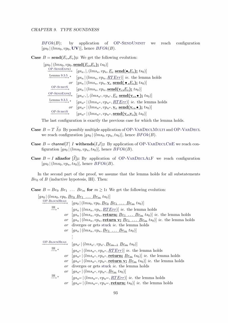
CHAPTER 9. TYPE SOUNDNESS

BFOk(B); by application of OP-SendUninit we reach configuration[gs0 | (lms0, vp0,UV)], hence BFOk(B).

Case B = send(Ec,Ev);: We get the following evolution:

[gs0 | (lms0, vp0, send(Ec,Ev); ts0)]OP-SendExpr1−−−−−−−−−−→ [gsa, |, (lmsa, vpa, Ec send(•,Ev); ts0)]Lemma 9.3.5−−−−−−−−→∗ [gsn | (lmsn, vpn, RTErr)] ie. the lemma holds

or [gsn | (lmsn, vpn,vc send( • ,Ev); ts0)]OP-SubstS−−−−−−−→ [gsn | (lmsn, vpn, send(vc,Ev); ts0)]

OP-SendExpr2−−−−−−−−−−→ [gsn′ , |, (lmsn′ , vpn′ , Ev send(vc, • ); ts0)]Lemma 9.3.5−−−−−−−−→∗ [gsn′′ | (lmsn′′ , vpn′′ , RTErr)] ie. the lemma holds

or [gsn′′ | (lmsn′′ , vpn′′ ,vv send(vc, • ); ts0)]OP-SubstS−−−−−−−→ [gsn′′ | (lmsn′′ , vpn′′ , send(vc,vv); ts0)]

The last configuration is exactly the previous case for which the lemma holds.

Case B = T I;: By possibly multiple application of OP-VarDeclMulti and OP-VarDeclwe reach configuration [gs0 | (lms0, vpn, ts0)], hence BFOk(B).

Case B = channel[T ] I withends[I,I];: By application of OP-VarDeclChE we reach con-figuration [gs0 | (lms0, vpn, ts0)], hence BFOk(B).

Case B = I aliasfor [I];: By application of OP-VarDeclAlF we reach configuration[gs0 | (lms0, vpn, ts0)], hence BFOk(B).

In the second part of the proof, we assume that the lemma holds for all substatementsBe0 of B (inductive hypotesis, IH). Then:

Case B = Be0 Be1 . . . Bem for m ≥ 1: We get the following evolution:

[gs0 | (lms0, vp0, Be0 Be1 . . . Bem ts0)]OP-BlockHead−−−−−−−−−−→ [gs0 | (lms0, vp0, Be0 Be1 . . . Bem ts0)]

IH−→∗ [gsn | (lmsn, vpn, RTErr)] ie. the lemma holdsor [gsn | (lmsn, vpn, return; Be1 . . . Bem ts0)] ie. the lemma holdsor [gsn | (lmsn, vpn, return v; Be1 . . . Bem ts0)] ie. the lemma holdsor diverges or gets stuck ie. the lemma holdsor [gsn | (lmsn, vpn, Be1 . . . Bem ts0)]

...OP-BlockHead−−−−−−−−−−→ [gsn′ | (lmsn′ , vpn′ , Bem−1 Bem ts0)]

IH−→∗ [gsn′′ | (lmsn′′ , vpn′′ , RTErr)] ie. the lemma holdsor [gsn′′ | (lmsn′′ , vpn′′ , return; Bem ts0)] ie. the lemma holdsor [gsn′′ | (lmsn′′ , vpn′′ , return v; Bem ts0)] ie. the lemma holdsor diverges or gets stuck ie. the lemma holdsor [gsn′′ | (lmsn′′ , vpn′′ , Bem ts0)]

IH−→∗ [gsn′′′ | (lmsn′′′ , vpn′′′ , RTErr)] ie. the lemma holdsor [gsn′′′ | (lmsn′′′ , vpn′′′ , return; ts0)] ie. the lemma holds

93

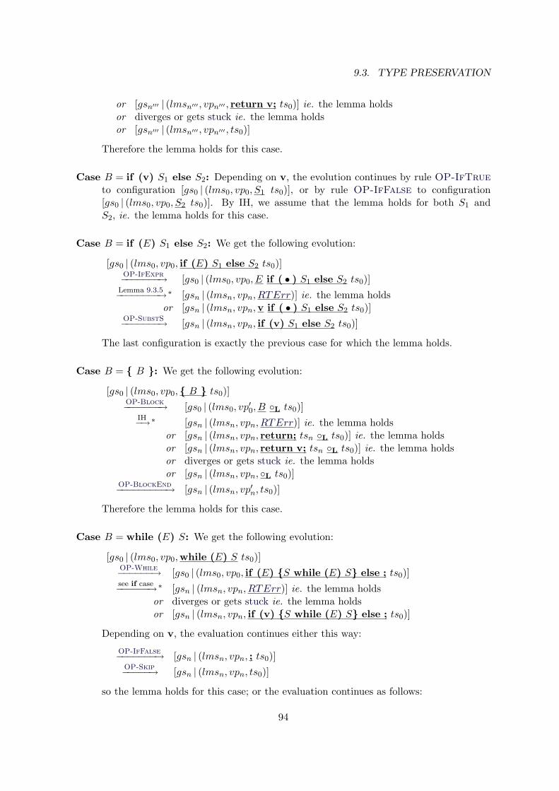
9.3. TYPE PRESERVATION

or [gsn′′′ | (lmsn′′′ , vpn′′′ , return v; ts0)] ie. the lemma holdsor diverges or gets stuck ie. the lemma holdsor [gsn′′′ | (lmsn′′′ , vpn′′′ , ts0)]

Therefore the lemma holds for this case.

Case B = if (v) S1 else S2: Depending on v, the evolution continues by rule OP-IfTrueto configuration [gs0 | (lms0, vp0, S1 ts0)], or by rule OP-IfFalse to configuration[gs0 | (lms0, vp0, S2 ts0)]. By IH, we assume that the lemma holds for both S1 andS2, ie. the lemma holds for this case.

Case B = if (E) S1 else S2: We get the following evolution:

[gs0 | (lms0, vp0, if (E) S1 else S2 ts0)]OP-IfExpr−−−−−−−→ [gs0 | (lms0, vp0, E if ( • ) S1 else S2 ts0)]

Lemma 9.3.5−−−−−−−−→∗ [gsn | (lmsn, vpn, RTErr)] ie. the lemma holdsor [gsn | (lmsn, vpn,v if ( • ) S1 else S2 ts0)]

OP-SubstS−−−−−−−→ [gsn | (lmsn, vpn, if (v) S1 else S2 ts0)]

The last configuration is exactly the previous case for which the lemma holds.

Case B = B : We get the following evolution:

[gs0 | (lms0, vp0, B ts0)]OP-Block−−−−−−−→ [gs0 | (lms0, vp′0, B L ts0)]

IH−→∗ [gsn | (lmsn, vpn, RTErr)] ie. the lemma holdsor [gsn | (lmsn, vpn, return; tsn L ts0)] ie. the lemma holdsor [gsn | (lmsn, vpn, return v; tsn L ts0)] ie. the lemma holdsor diverges or gets stuck ie. the lemma holdsor [gsn | (lmsn, vpn, L ts0)]

OP-BlockEnd−−−−−−−−−→ [gsn | (lmsn, vp′n, ts0)]

Therefore the lemma holds for this case.

Case B = while (E) S: We get the following evolution:

[gs0 | (lms0, vp0,while (E) S ts0)]OP-While−−−−−−→ [gs0 | (lms0, vp0, if (E) S while (E) S else ; ts0)]see if case−−−−−−→∗ [gsn | (lmsn, vpn, RTErr)] ie. the lemma holds

or diverges or gets stuck ie. the lemma holdsor [gsn | (lmsn, vpn, if (v) S while (E) S else ; ts0)]

Depending on v, the evaluation continues either this way:

OP-IfFalse−−−−−−−→ [gsn | (lmsn, vpn, ; ts0)]OP-Skip−−−−−→ [gsn | (lmsn, vpn, ts0)]

so the lemma holds for this case; or the evaluation continues as follows:

94

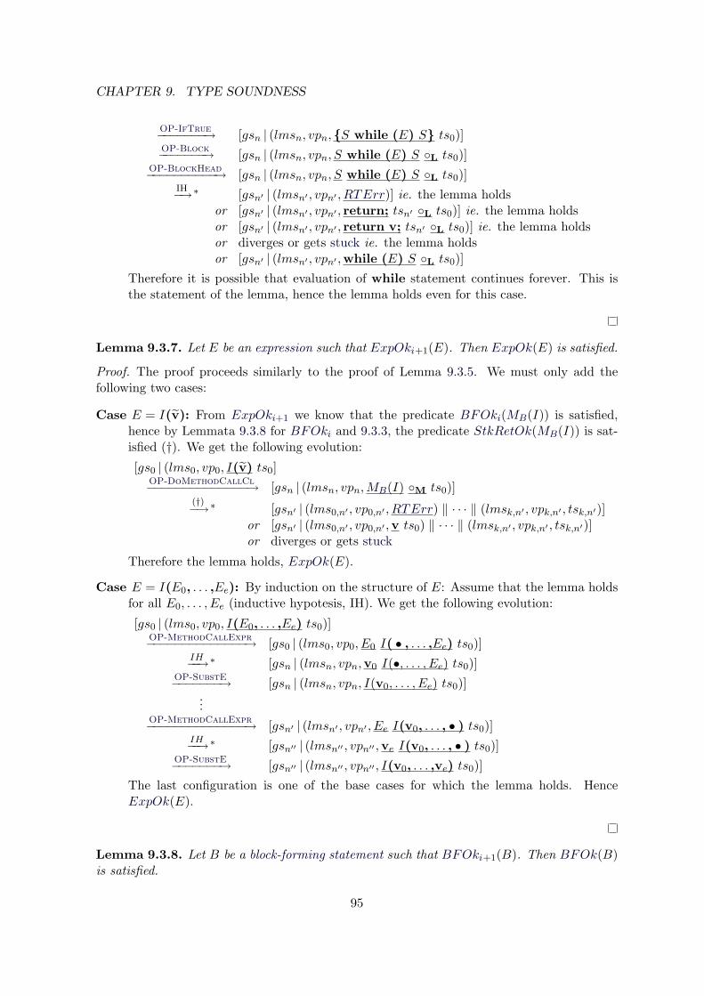
CHAPTER 9. TYPE SOUNDNESS

OP-IfTrue−−−−−−−→ [gsn | (lmsn, vpn,S while (E) S ts0)]OP-Block−−−−−−−→ [gsn | (lmsn, vpn, S while (E) S L ts0)]

OP-BlockHead−−−−−−−−−−→ [gsn | (lmsn, vpn, S while (E) S L ts0)]IH−→∗ [gsn′ | (lmsn′ , vpn′ , RTErr)] ie. the lemma holds

or [gsn′ | (lmsn′ , vpn′ , return; tsn′ L ts0)] ie. the lemma holdsor [gsn′ | (lmsn′ , vpn′ , return v; tsn′ L ts0)] ie. the lemma holdsor diverges or gets stuck ie. the lemma holdsor [gsn′ | (lmsn′ , vpn′ ,while (E) S L ts0)]

Therefore it is possible that evaluation of while statement continues forever. This isthe statement of the lemma, hence the lemma holds even for this case.

Lemma 9.3.7. Let E be an expression such that ExpOki+1(E). Then ExpOk(E) is satisfied.

Proof. The proof proceeds similarly to the proof of Lemma 9.3.5. We must only add thefollowing two cases:

Case E = I(v): From ExpOki+1 we know that the predicate BFOki(MB(I)) is satisfied,hence by Lemmata 9.3.8 for BFOki and 9.3.3, the predicate StkRetOk(MB(I)) is sat-isfied (†). We get the following evolution:

[gs0 | (lms0, vp0, I(v) ts0]OP-DoMethodCallCl−−−−−−−−−−−−−−→ [gsn | (lmsn, vpn,MB(I) M ts0)]

(†)−→∗ [gsn′ | (lms0,n′ , vp0,n′ , RTErr) ‖ · · · ‖ (lmsk,n′ , vpk,n′ , tsk,n′)]or [gsn′ | (lms0,n′ , vp0,n′ ,v ts0) ‖ · · · ‖ (lmsk,n′ , vpk,n′ , tsk,n′)]or diverges or gets stuck

Therefore the lemma holds, ExpOk(E).

Case E = I(E0, . . . ,Ee): By induction on the structure of E: Assume that the lemma holdsfor all E0, . . . , Ee (inductive hypotesis, IH). We get the following evolution:

[gs0 | (lms0, vp0, I(E0, . . . ,Ee) ts0)]OP-MethodCallExpr−−−−−−−−−−−−−−→ [gs0 | (lms0, vp0, E0 I( • , . . . ,Ee) ts0)]

IH−−→∗ [gsn | (lmsn, vpn,v0 I(•, . . . , Ee) ts0)]OP-SubstE−−−−−−−→ [gsn | (lmsn, vpn, I(v0, . . . , Ee) ts0)]

...OP-MethodCallExpr−−−−−−−−−−−−−−→ [gsn′ | (lmsn′ , vpn′ , Ee I(v0, . . . , • ) ts0)]

IH−−→∗ [gsn′′ | (lmsn′′ , vpn′′ ,ve I(v0, . . . , • ) ts0)]OP-SubstE−−−−−−−→ [gsn′′ | (lmsn′′ , vpn′′ , I(v0, . . . ,ve) ts0)]

The last configuration is one of the base cases for which the lemma holds. HenceExpOk(E).

Lemma 9.3.8. Let B be a block-forming statement such that BFOki+1(B). Then BFOk(B)is satisfied.

95

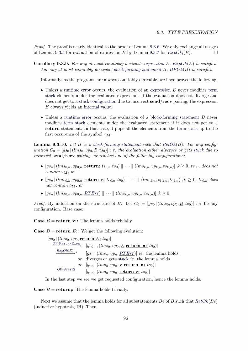
9.3. TYPE PRESERVATION

Proof. The proof is nearly identical to the proof of Lemma 9.3.6. We only exchange all usagesof Lemma 9.3.5 for evaluation of expression E by Lemma 9.3.7 for ExpOki(E).

Corollary 9.3.9. For any at most countably derivable expression E, ExpOk(E) is satisfied.For any at most countably derivable block-forming statement B, BFOk(B) is satisfied.

Informally, as the programs are always countably derivable, we have proved the following:

• Unless a runtime error occurs, the evaluation of an expression E never modifies termstack elements under the evaluated expression. If the evaluation does not diverge anddoes not get to a stuck configuration due to incorrect send/recv pairing, the expressionE always yields an internal value,

• Unless a runtime error occurs, the evaluation of a block-forming statement B nevermodifies term stack elements under the evaluated statement if it does not get to areturn statement. In that case, it pops all the elements from the term stack up to thefirst occurence of the symbol M.

Lemma 9.3.10. Let B be a block-forming statement such that RetOk(B). For any config-uration C0 = [gs0 | (lms0, vp0, B ts0)] : τ , the evaluation either diverges or gets stuck due toincorrect send/recv pairing, or reaches one of the following configurations:

• [gsn | (lms0,n, vp0,n, return; ts0,n ts0) ‖ · · · ‖ (lmsk,n, vpk,n, tsk,n)], k ≥ 0, ts0,n does notcontain M, or

• [gsn | (lms0,n, vp0,n, return v; ts0,n ts0) ‖ · · · ‖ (lmsk,n, vpk,n, tsk,n)], k ≥ 0, ts0,n doesnot contain M, or

• [gsn | (lms0,n, vp0,n, RTErr) ‖ · · · ‖ (lmsk,n, vpk,n, tsk,n)], k ≥ 0.

Proof. By induction on the structure of B. Let C0 = [gs0 | (lms0, vp0, B ts0)] : τ be anyconfiguration. Base case:

Case B = return v;: The lemma holds trivially.

Case B = return E;: We get the following evolution:

[gs0 | (lms0, vp0, return E; ts0)]OP-ReturnExpr−−−−−−−−−−−→ [gs0, |, (lms0, vp0, E return • ; ts0)]ExpOk(E)−−−−−−→∗ [gsn | (lmsn, vpn, RTErr)] ie. the lemma holds

or diverges or gets stuck ie. the lemma holdsor [gsn | (lmsn, vpn,v return • ; ts0)]

OP-SubstS−−−−−−−→ [gsn | (lmsn, vpn, return v; ts0)]

In the last step we see we get requested configuration, hence the lemma holds.

Case B = return;: The lemma holds trivially.

Next we assume that the lemma holds for all substatements Be of B such that RetOk(Be)(inductive hypotesis, IH). Then:

96

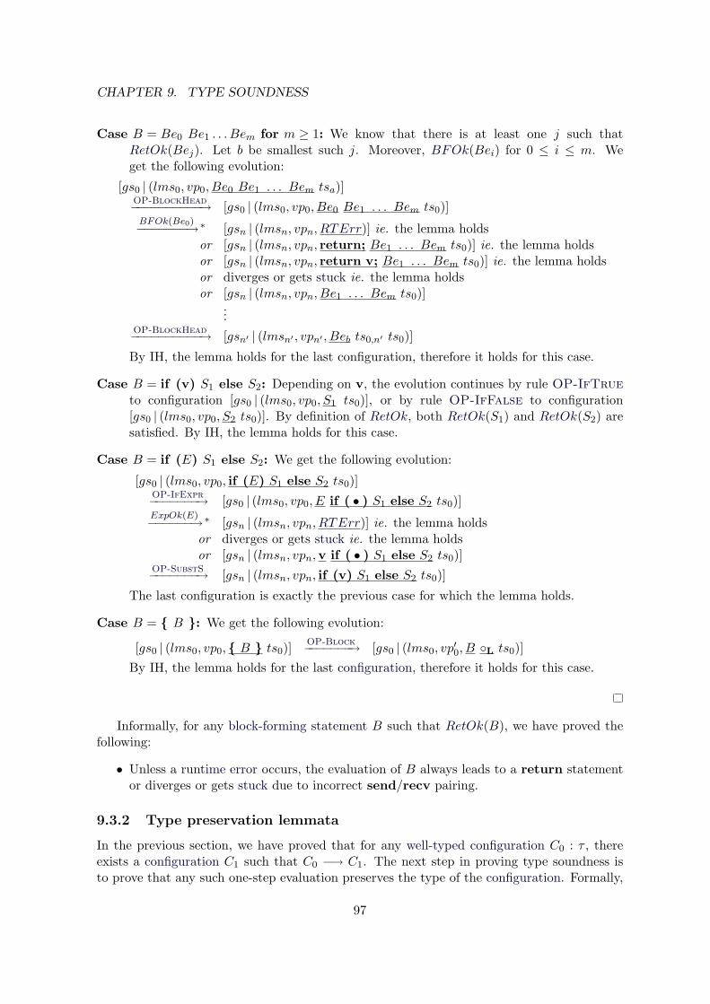
CHAPTER 9. TYPE SOUNDNESS

Case B = Be0 Be1 . . . Bem for m ≥ 1: We know that there is at least one j such thatRetOk(Bej). Let b be smallest such j. Moreover, BFOk(Bei) for 0 ≤ i ≤ m. Weget the following evolution:

[gs0 | (lms0, vp0, Be0 Be1 . . . Bem tsa)]OP-BlockHead−−−−−−−−−−→ [gs0 | (lms0, vp0, Be0 Be1 . . . Bem ts0)]BFOk(Be0)−−−−−−−→∗ [gsn | (lmsn, vpn, RTErr)] ie. the lemma holds

or [gsn | (lmsn, vpn, return; Be1 . . . Bem ts0)] ie. the lemma holdsor [gsn | (lmsn, vpn, return v; Be1 . . . Bem ts0)] ie. the lemma holdsor diverges or gets stuck ie. the lemma holdsor [gsn | (lmsn, vpn, Be1 . . . Bem ts0)]

...OP-BlockHead−−−−−−−−−−→ [gsn′ | (lmsn′ , vpn′ , Beb ts0,n′ ts0)]

By IH, the lemma holds for the last configuration, therefore it holds for this case.

Case B = if (v) S1 else S2: Depending on v, the evolution continues by rule OP-IfTrueto configuration [gs0 | (lms0, vp0, S1 ts0)], or by rule OP-IfFalse to configuration[gs0 | (lms0, vp0, S2 ts0)]. By definition of RetOk, both RetOk(S1) and RetOk(S2) aresatisfied. By IH, the lemma holds for this case.

Case B = if (E) S1 else S2: We get the following evolution:

[gs0 | (lms0, vp0, if (E) S1 else S2 ts0)]OP-IfExpr−−−−−−−→ [gs0 | (lms0, vp0, E if ( • ) S1 else S2 ts0)]ExpOk(E)−−−−−−→∗ [gsn | (lmsn, vpn, RTErr)] ie. the lemma holds

or diverges or gets stuck ie. the lemma holdsor [gsn | (lmsn, vpn,v if ( • ) S1 else S2 ts0)]

OP-SubstS−−−−−−−→ [gsn | (lmsn, vpn, if (v) S1 else S2 ts0)]

The last configuration is exactly the previous case for which the lemma holds.

Case B = B : We get the following evolution:

[gs0 | (lms0, vp0, B ts0)]OP-Block−−−−−−−→ [gs0 | (lms0, vp′0, B L ts0)]

By IH, the lemma holds for the last configuration, therefore it holds for this case.

Informally, for any block-forming statement B such that RetOk(B), we have proved thefollowing:

• Unless a runtime error occurs, the evaluation of B always leads to a return statementor diverges or gets stuck due to incorrect send/recv pairing.

9.3.2 Type preservation lemmata

In the previous section, we have proved that for any well-typed configuration C0 : τ , thereexists a configuration C1 such that C0 −→ C1. The next step in proving type soundness isto prove that any such one-step evaluation preserves the type of the configuration. Formally,

97

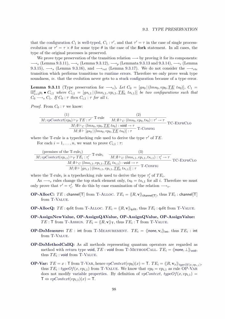
9.3. TYPE PRESERVATION

that the configuration C1 is well-typed, C1 : τ ′, and that τ ′ = τ in the case of single process-evolution or τ ′ = τ × θ for some type θ in the case of the fork statement. In all cases, thetype of the original processes is preserved.

We prove type preservation of the transition relation −→ by proving it for its components:−→v (Lemma 9.3.11), −→e (Lemma 9.3.12), −→p (Lemmata 9.3.13 and 9.3.14), −→r (Lemma9.3.15), −→s (Lemma 9.3.16), and −→ret (Lemma 9.3.17). We do not consider the −→rte

transition which performs transitions to runtime errors. Therefore we only prove weak typesoundness, ie. that the evolution never gets to a stuck configuration because of a type error.

Lemma 9.3.11 (Type preservation for −→v). Let C0 = [gs0 | (lms0, vp0, TE ts0)], C1 =qi=1pi • Ci,1 where Ci,1 = [gsi,1 | (lmsi,1, vpi,1, TEi tsi,1)] be two configurations such that

C0 −→v C1. If C0 : τ then Ci,1 : τ for all i.

Proof. From C0 : τ we know:

(1)T-rule

M ; vpContext(vp0) `T TE : τ ′(2)

M ; ∅ `C (lms0, vp0, ts0) : τ ′ → τTC-ExprClo

M ; ∅ `C (lms0, vp0, TE ts0) : void→ τT-Config

M ; ∅ ` [gs0 | (lms0, vp0, TE ts0)] : τ

where the T-rule is a typechecking rule used to derive the type τ ′ of TE.For each i = 1, . . . , n, we want to prove Ci,1 : τ :

(premises of the T-rulei) T-ruleiM ; vpContext(vpi,1) `T TEi : τ ′

i

(3)M ; ∅ `C (lmsi,1, vpi,1, tsi,1) : τ ′

i → τTC-ExprClo

M ; ∅ `C (lmsi,1, vpi,1, TEi tsi,1) : void→ τT-Config

M ; ∅ ` [gsi,1 | (lmsi,1, vpi,1, TEi tsi,1)] : τ

where the T-rulei is a typechecking rule used to derive the type τ ′i of TEi.As −→v rules change the top stack element only, ts0 = tsi,1 for all i. Therefore we must

only prove that τ ′ = τ ′i . We do this by case examination of the relation −→v.

OP-AllocC: TE : channel[T] from T-Alloc. TEi = 〈〈R,v〉〉channel[T], thus TEi : channel[T]from T-Value.

OP-AllocQ: TE : qd it from T-Alloc. TEi = 〈〈R,v〉〉qd it, thus TEi : qd it from T-Value.

OP-AssignNewValue, OP-AssignQAValue, OP-AssignQValue, OP-AssignValue:TE : T from T-Assign. TEi = 〈〈R,v〉〉T, thus TEi : T from T-Value.

OP-DoMeasure: TE : int from T-Measurement. TEi = 〈〈none,vi〉〉int, thus TEi : intfrom T-Value.

OP-DoMethodCallQ: As all methods representing quantum operators are regarded asmethod with return type void, TE : void from T-MethodCall. TEi = 〈〈none,⊥〉〉void,thus TEi : void from T-Value.

OP-Var: TE = x : T from T-Var, hence vpContext(vp0)(x) = T. TEi = 〈〈R,vx〉〉typeOf (x ,vpi,1 ),thus TEi : typeOf(x, vpi,1) from T-Value. We know that vp0 = vpi,1 as rule OP-Vardoes not modify variable properties. By definition of vpContext, typeOf(x, vpi,1) =T⇔ vpContext(vpi,1)(x) = T.

98

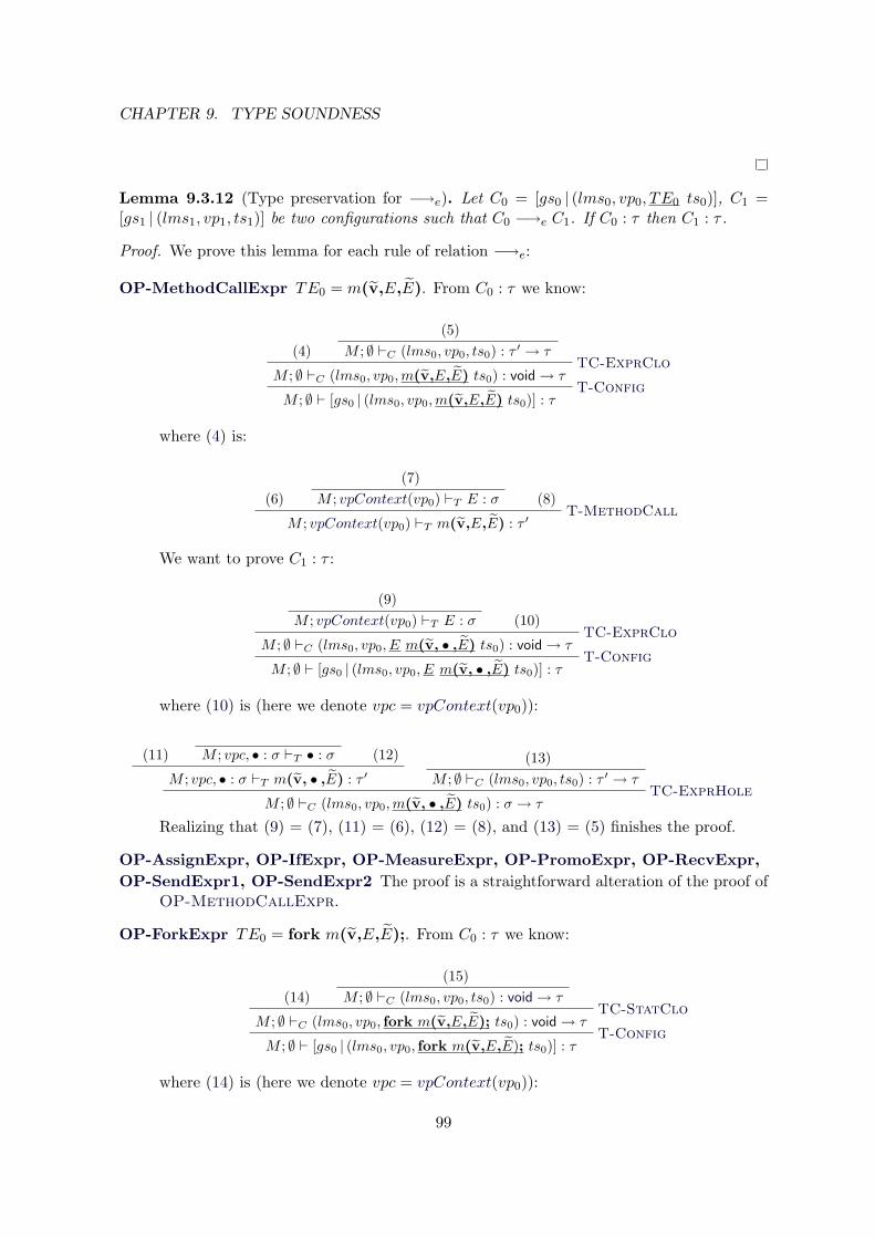
CHAPTER 9. TYPE SOUNDNESS

Lemma 9.3.12 (Type preservation for −→e). Let C0 = [gs0 | (lms0, vp0, TE0 ts0)], C1 =[gs1 | (lms1, vp1, ts1)] be two configurations such that C0 −→e C1. If C0 : τ then C1 : τ .

Proof. We prove this lemma for each rule of relation −→e:

OP-MethodCallExpr TE0 = m(v,E,E). From C0 : τ we know:

(4)(5)

M ; ∅ `C (lms0, vp0, ts0) : τ ′ → τTC-ExprClo

M ; ∅ `C (lms0, vp0,m(v,E,E) ts0) : void→ τT-Config

M ; ∅ ` [gs0 | (lms0, vp0,m(v,E,E) ts0)] : τ

where (4) is:

(6)(7)

M ; vpContext(vp0) `T E : σ (8)T-MethodCall

M ; vpContext(vp0) `T m(v,E,E) : τ ′

We want to prove C1 : τ :

(9)M ; vpContext(vp0) `T E : σ (10)

TC-ExprCloM ; ∅ `C (lms0, vp0, E m(v, • ,E) ts0) : void→ τ

T-ConfigM ; ∅ ` [gs0 | (lms0, vp0, E m(v, • ,E) ts0)] : τ

where (10) is (here we denote vpc = vpContext(vp0)):

(11) M ; vpc, • : σ `T • : σ (12)

M ; vpc, • : σ `T m(v, • ,E) : τ ′(13)

M ; ∅ `C (lms0, vp0, ts0) : τ ′ → τTC-ExprHole

M ; ∅ `C (lms0, vp0,m(v, • ,E) ts0) : σ → τ

Realizing that (9) = (7), (11) = (6), (12) = (8), and (13) = (5) finishes the proof.

OP-AssignExpr, OP-IfExpr, OP-MeasureExpr, OP-PromoExpr, OP-RecvExpr,OP-SendExpr1, OP-SendExpr2 The proof is a straightforward alteration of the proof of

OP-MethodCallExpr.

OP-ForkExpr TE0 = fork m(v,E,E);. From C0 : τ we know:

(14)(15)

M ; ∅ `C (lms0, vp0, ts0) : void→ τTC-StatClo

M ; ∅ `C (lms0, vp0, fork m(v,E,E); ts0) : void→ τT-Config

M ; ∅ ` [gs0 | (lms0, vp0, fork m(v,E,E); ts0)] : τ

where (14) is (here we denote vpc = vpContext(vp0)):

99

9.3. TYPE PRESERVATION

(16)(17)

M ; vpc `T E : σ (18)T-MethodCall

M ; vpc `T m(v,E,E); : τ ′ m is a classical methodT-Fork

M ; vpc `T fork m(v,E,E); : void

We want to prove C1 : τ :

(19)M ; vpContext(vp0) `T E : σ (20)

TC-ExprCloM ; ∅ `C (lms0, vp0, E fork m(v, • ,E); ts0) : void→ τ

T-ConfigM ; ∅ ` [gs0 | (lms0, vp0, E fork m(v, • ,E); ts0)] : τ

where (20) is (here we denote vpc = vpContext(vp0)):

(21) M ; vpc, • : σ `T • : σ (22)

M ; vpc, • : σ `T m(v, • ,E); : τ ′

M ; vpc, • : σ `T fork m(v, • ,E); : void

(23)M ; ∅ `C (lms0, vp0, ts0) : void→ τ

TC-StatHoleM ; ∅ `C (lms0, vp0, fork m(v, • ,E); ts0) : σ → τ

Realizing that (19) = (17), (22) = (18), (21) = (16), and (23) = (15) finishes the proof.

OP-ReturnExpr TE0 = return E;. We know that vp0 = vp1 = [vpG G vp], ts0 =. . . M tsr. Denote by ρ = typeOf(@retV al, vp1). From C0 : τ we know:

(24)M ; vpContext(vp0) `T E : ρ

(25)M ; ∅ `C (lms0, vpG, tsr) : ρ→ τ

TC-RetExprM ; ∅ `C (lms0, vp0, return E; . . . M tsr) : void→ τ

T-ConfigM ; ∅ ` [gs0 | (lms0, vp0, return E; . . . M tsr)] : τ

We want to prove C1 : τ :

(26)M ; vpContext(vp0) `T E : ρ (27)

TC-ExprCloM ; ∅ `C (lms0, vp0, E return • ; . . . M tsr) : void→ τ

T-ConfigM ; ∅ ` [gs0 | (lms0, vp0, E return • ; . . . M tsr)] : τ

where (27) is:

(28)M ; ∅ `C (lms0, vpG, tsr) : ρ→ τ

TC-RetHoleM ; ∅ `C (lms0, vp0, return • ; . . . M tsr) : void→ τ

Realizing that (26) = (24), and (28) = (25) finishes the proof.

OP-DoMethodCallCl TE0 = m(v). From C0 : τ we know:

(29)(30)

M ; ∅ `C (lms0, vp0, ts0) : τ ′ → τTC-ExprClo

M ; ∅ `C (lms0, vp0,m(v0, . . . ,vn) ts0) : void→ τT-Config

M ; ∅ ` [gs0 | (lms0, vp0,m(v0, . . . ,vn) ts0)] : τ

100

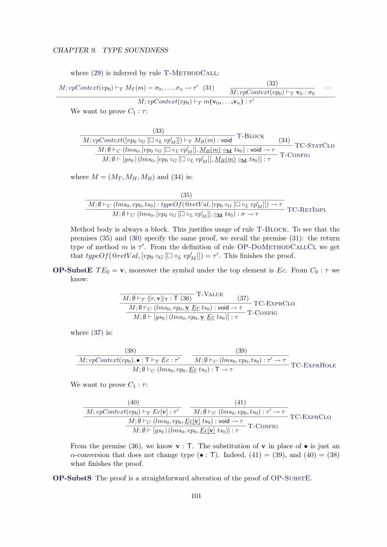
CHAPTER 9. TYPE SOUNDNESS

where (29) is inferred by rule T-MethodCall:

M ; vpContext(vp0) `T MT (m) = σ0, . . . , σn → τ ′ (31)(32)

M ; vpContext(vp0) `T v0 : σ0· · ·

M ; vpContext(vp0) `T m(v0, . . . ,vn) : τ ′

We want to prove C1 : τ :

(33)T-Block

M ; vpContext([vp0 G [ L vp′M ]]) `T MB(m) : void (34)

TC-StatCloM ; ∅ `C (lms0, [vp0 G [ L vp′

M ]],MB(m) M ts0) : void→ τT-Config

M ; ∅ ` [gs0 | (lms0, [vp0 G [ L vp′M ]],MB(m) M ts0)] : τ

where M = (MT ,MH ,MB) and (34) is:

(35)M ; ∅ `C (lms0, vp0, ts0) : typeOf(@retV al, [vp0 G [ L vp′

M ]])→ τTC-RetImpl

M ; ∅ `C (lms0, [vp0 G [ L vp′M ]], M ts0) : σ → τ

Method body is always a block. This justifies usage of rule T-Block. To see that thepremises (35) and (30) specify the same proof, we recall the premise (31): the returntype of method m is τ ′. From the definition of rule OP-DoMethodCallCl we getthat typeOf(@retV al, [vp0 G [ L vp′M ]]) = τ ′. This finishes the proof.

OP-SubstE TE0 = v, moreover the symbol under the top element is Ec. From C0 : τ weknow:

T-ValueM ; ∅ `T 〈〈r,v〉〉T : T (36) (37)

TC-ExprCloM ; ∅ `C (lms0, vp0,v Ec ts0) : void→ τ

T-ConfigM ; ∅ ` [gs0 | (lms0, vp0,v Ec ts0)] : τ

where (37) is:

(38)M ; vpContext(vp0), • : T `T Ec : τ ′

(39)M ; ∅ `C (lms0, vp0, ts0) : τ ′ → τ

TC-ExprHoleM ; ∅ `C (lms0, vp0, Ec ts0) : T→ τ

We want to prove C1 : τ :

(40)M ; vpContext(vp0) `T Ec[v] : τ ′

(41)M ; ∅ `C (lms0, vp0, ts0) : τ ′ → τ

TC-ExprCloM ; ∅ `C (lms0, vp0, Ec[v] ts0) : void→ τ

T-ConfigM ; ∅ ` [gs0 | (lms0, vp0, Ec[v] ts0)] : τ

From the premise (36), we know v : T. The substitution of v in place of • is just anα-conversion that does not change type (• : T). Indeed, (41) = (39), and (40) = (38)what finishes the proof.

OP-SubstS The proof is a straightforward alteration of the proof of OP-SubstE.

101

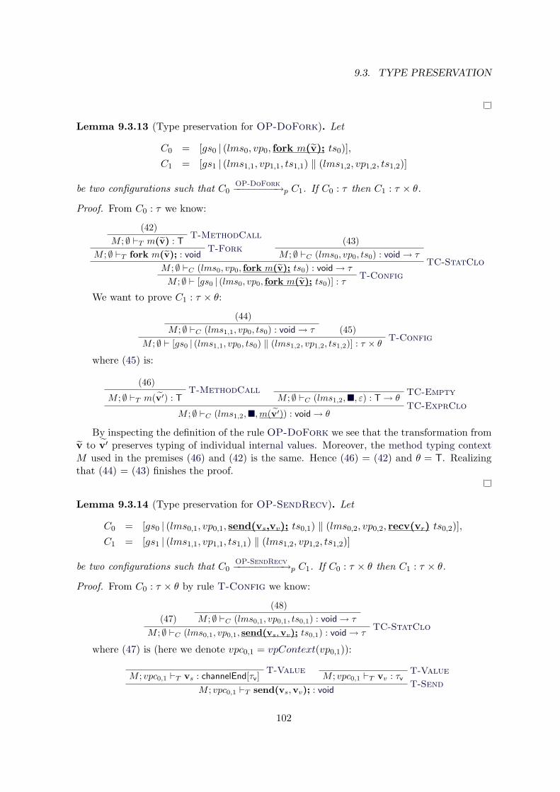
9.3. TYPE PRESERVATION

Lemma 9.3.13 (Type preservation for OP-DoFork). Let

C0 = [gs0 | (lms0, vp0, fork m(v); ts0)],C1 = [gs1 | (lms1,1, vp1,1, ts1,1) ‖ (lms1,2, vp1,2, ts1,2)]

be two configurations such that C0OP-DoFork−−−−−−−−→p C1. If C0 : τ then C1 : τ × θ.

Proof. From C0 : τ we know:

(42)T-MethodCall

M ; ∅ `T m(v) : TT-Fork

M ; ∅ `T fork m(v); : void

(43)M ; ∅ `C (lms0, vp0, ts0) : void→ τ

TC-StatCloM ; ∅ `C (lms0, vp0, fork m(v); ts0) : void→ τ

T-ConfigM ; ∅ ` [gs0 | (lms0, vp0, fork m(v); ts0)] : τ

We want to prove C1 : τ × θ:

(44)M ; ∅ `C (lms1,1, vp0, ts0) : void→ τ (45)

T-ConfigM ; ∅ ` [gs0 | (lms1,1, vp0, ts0) ‖ (lms1,2, vp1,2, ts1,2)] : τ × θ

where (45) is:

(46)T-MethodCall

M ; ∅ `T m(v′) : TTC-Empty

M ; ∅ `C (lms1,2,, ε) : T→ θTC-ExprClo

M ; ∅ `C (lms1,2,,m(v′)) : void→ θ

By inspecting the definition of the rule OP-DoFork we see that the transformation fromv to v′ preserves typing of individual internal values. Moreover, the method typing contextM used in the premises (46) and (42) is the same. Hence (46) = (42) and θ = T. Realizingthat (44) = (43) finishes the proof.

Lemma 9.3.14 (Type preservation for OP-SendRecv). Let

C0 = [gs0 | (lms0,1, vp0,1, send(vs,vv); ts0,1) ‖ (lms0,2, vp0,2, recv(vr) ts0,2)],C1 = [gs1 | (lms1,1, vp1,1, ts1,1) ‖ (lms1,2, vp1,2, ts1,2)]

be two configurations such that C0OP-SendRecv−−−−−−−−−→p C1. If C0 : τ × θ then C1 : τ × θ.

Proof. From C0 : τ × θ by rule T-Config we know:

(47)(48)

M ; ∅ `C (lms0,1, vp0,1, ts0,1) : void→ τTC-StatClo

M ; ∅ `C (lms0,1, vp0,1, send(vs,vv); ts0,1) : void→ τ

where (47) is (here we denote vpc0,1 = vpContext(vp0,1)):

T-ValueM ; vpc0,1 `T vs : channelEnd[τv]

T-ValueM ; vpc0,1 `T vv : τv

T-SendM ; vpc0,1 `T send(vs,vv); : void

102

CHAPTER 9. TYPE SOUNDNESS

and (here we denote vpc0,2 = vpContext(vp0,2)):

T-ValueM ; vpc0,2 `T vr : channelEnd[θ′]

T-RecvM ; vpc0,2 `T recv(vr) : θ′

(49)M ; ∅ `C (lms0,1, vp0,2, ts0,2) : θ′ → θ

TC-ExprCloM ; ∅ `C (lms0,2, vp0,2, recv(vr) ts0,2) : void→ θ

We want to prove C1 : τ × θ:

(50)M ; ∅ `C (lms1,1, vp0,1, ts0,1) : void→ τ (51)

T-ConfigM ; ∅ ` [gs0 | (lms1,1, vp0,1, ts0,1) ‖ (lms1,2, vp1,2,vv ts1,2)] : τ × θ

where (51) is (here we denote vpc1,2 = vpContext(vp1,2)):

T-ValueM ; vpc1,2 `T vv : θ′′

(52)M ; ∅ `C (lms1,2, vp0,2, ts0,2) : θ′′ → θ

TC-ExprCloM ; ∅ `C (lms1,2, vp0,2,vv ts0,2) : void→ θ

By inspecting the definition of rule OP-SendRecv we see that vs and vr are ends of thesame channel, hence their types match. Therefore, θ′ = τv. Indeed, θ′′ = τv. As changes inlocal memory state do not change type of internal values, (52) = (49). Realizing that (50) =(48) finishes the proof.

Lemma 9.3.15 (Type preservation for −→r). Let C0 = [gs0 | (lms0, vp0, TE0 ts0)], C1 =[gs1 | (lms1, vp1, ts1)] be two configurations such that C0 −→r C1. If C0 : τ then C1 : τ .

Proof. We prove this lemma for each rule of relation −→r:

OP-BlockHead TE0 = Be = Be0 Be1 . . . Ben where n ≥ 1. From C0 : τ we know:

(53)M ; ∅ `C (lms0, vp0, Be0 Be1 . . . Ben ts0) : void→ τ

TC-BlockHeadM ; ∅ `C (lms0, vp0, Be ts0) : void→ τ

T-ConfigM ; ∅ ` [gs0 | (lms0, vp0, Be ts0)] : τ

We want to prove C1 : τ :

(54)M ; ∅ `C (lms0, vp0, Be0 Be1 . . . Ben ts0) : void→ τ

T-ConfigM ; ∅ ` [gs0 | (lms0, vp0, Be0 Be1 . . . Ben ts0)] : τ

Indeed, (53) = (54).

103

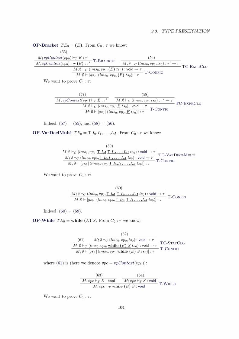
9.3. TYPE PRESERVATION

OP-Bracket TE0 = (E). From C0 : τ we know:(55)

M ; vpContext(vp0) `T E : τ ′T-Bracket

M ; vpContext(vp0) `T (E) : τ ′(56)

M ; ∅ `C (lms0, vp0, ts0) : τ ′ → τTC-ExprClo

M ; ∅ `C (lms0, vp0, (E) ts0) : void→ τT-Config

M ; ∅ ` [gs0 | (lms0, vp0, (E) ts0)] : τ

We want to prove C1 : τ :

(57)M ; vpContext(vp0) `T E : τ ′

(58)M ; ∅ `C (lms0, vp0, ts0) : τ ′ → τ

TC-ExprCloM ; ∅ `C (lms0, vp0, E ts0) : void→ τ

T-ConfigM ; ∅ ` [gs0 | (lms0, vp0, E ts0)] : τ

Indeed, (57) = (55), and (58) = (56).

OP-VarDeclMulti TE0 = T I0,I1, . . . ,In;. From C0 : τ we know:

(59)M ; ∅ `C (lms0, vp0,T I0; T I1, . . . ,In; ts0) : void→ τ

TC-VarDeclMultiM ; ∅ `C (lms0, vp0,T I0,I1, . . . , In; ts0) : void→ τ

T-ConfigM ; ∅ ` [gs0 | (lms0, vp0,T I0,I1, . . . ,In; ts0)] : τ

We want to prove C1 : τ :

(60)M ; ∅ `C (lms0, vp0,T I0; T I1, . . . ,In; ts0) : void→ τ

T-ConfigM ; ∅ ` [gs0 | (lms0, vp0,T I0; T I1, . . . ,In; ts0)] : τ

Indeed, (60) = (59).

OP-While TE0 = while (E) S. From C0 : τ we know:

(61)(62)

M ; ∅ `C (lms0, vp0, ts0) : void→ τTC-StatClo

M ; ∅ `C (lms0, vp0,while (E) S ts0) : void→ τT-Config

M ; ∅ ` [gs0 | (lms0, vp0,while (E) S ts0)] : τ

where (61) is (here we denote vpc = vpContext(vp0)):

(63)M ; vpc `T E : bool

(64)M ; vpc `T S : void

T-WhileM ; vpc `T while (E) S : void

We want to prove C1 : τ :

104

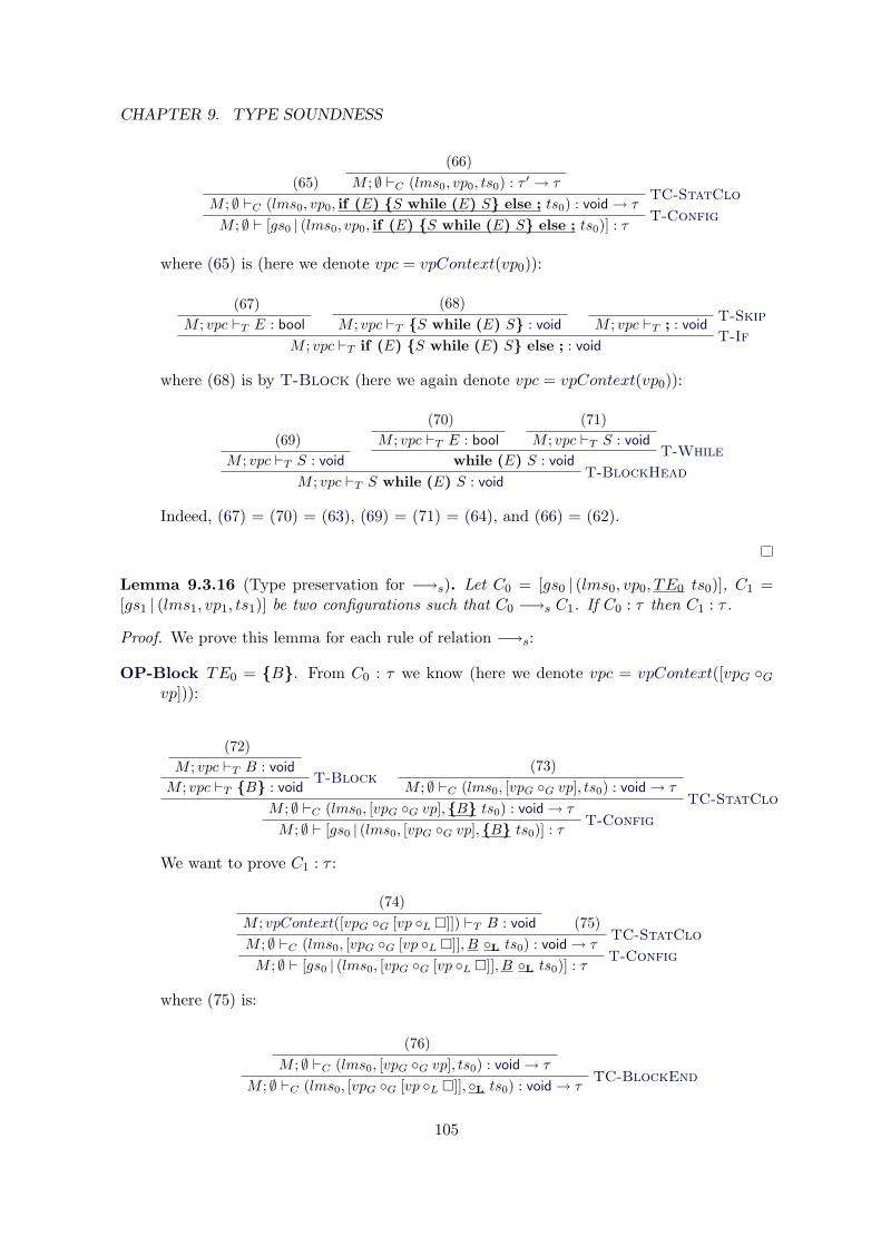
CHAPTER 9. TYPE SOUNDNESS

(65)(66)

M ; ∅ `C (lms0, vp0, ts0) : τ ′ → τTC-StatClo

M ; ∅ `C (lms0, vp0, if (E) S while (E) S else ; ts0) : void→ τT-Config

M ; ∅ ` [gs0 | (lms0, vp0, if (E) S while (E) S else ; ts0)] : τ

where (65) is (here we denote vpc = vpContext(vp0)):

(67)M ; vpc `T E : bool

(68)M ; vpc `T S while (E) S : void

T-SkipM ; vpc `T ; : void

T-IfM ; vpc `T if (E) S while (E) S else ; : void

where (68) is by T-Block (here we again denote vpc = vpContext(vp0)):

(69)M ; vpc `T S : void

(70)M ; vpc `T E : bool

(71)M ; vpc `T S : void

T-Whilewhile (E) S : void

T-BlockHeadM ; vpc `T S while (E) S : void

Indeed, (67) = (70) = (63), (69) = (71) = (64), and (66) = (62).

Lemma 9.3.16 (Type preservation for −→s). Let C0 = [gs0 | (lms0, vp0, TE0 ts0)], C1 =[gs1 | (lms1, vp1, ts1)] be two configurations such that C0 −→s C1. If C0 : τ then C1 : τ .

Proof. We prove this lemma for each rule of relation −→s:

OP-Block TE0 = B. From C0 : τ we know (here we denote vpc = vpContext([vpG Gvp])):

(72)M ; vpc `T B : void

T-BlockM ; vpc `T B : void

(73)M ; ∅ `C (lms0, [vpG G vp], ts0) : void→ τ

TC-StatCloM ; ∅ `C (lms0, [vpG G vp],B ts0) : void→ τ

T-ConfigM ; ∅ ` [gs0 | (lms0, [vpG G vp],B ts0)] : τ

We want to prove C1 : τ :

(74)M ; vpContext([vpG G [vp L ]]) `T B : void (75)

TC-StatCloM ; ∅ `C (lms0, [vpG G [vp L ]], B L ts0) : void→ τ

T-ConfigM ; ∅ ` [gs0 | (lms0, [vpG G [vp L ]], B L ts0)] : τ

where (75) is:

(76)M ; ∅ `C (lms0, [vpG G vp], ts0) : void→ τ

TC-BlockEndM ; ∅ `C (lms0, [vpG G [vp L ]], L ts0) : void→ τ

105

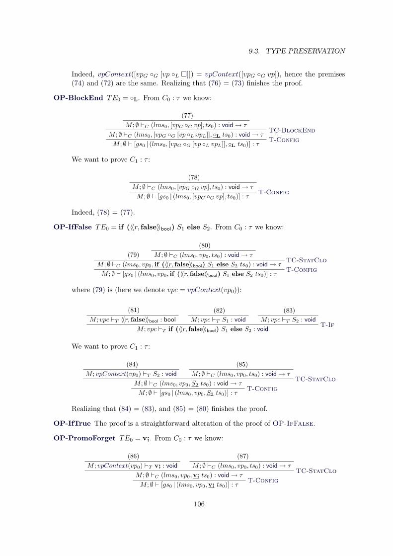
9.3. TYPE PRESERVATION

Indeed, vpContext([vpG G [vp L ]]) = vpContext([vpG G vp]), hence the premises(74) and (72) are the same. Realizing that (76) = (73) finishes the proof.

OP-BlockEnd TE0 = L. From C0 : τ we know:

(77)M ; ∅ `C (lms0, [vpG G vp], ts0) : void→ τ

TC-BlockEndM ; ∅ `C (lms0, [vpG G [vp L vpL]], L ts0) : void→ τ

T-ConfigM ; ∅ ` [gs0 | (lms0, [vpG G [vp L vpL]], L ts0)] : τ

We want to prove C1 : τ :

(78)M ; ∅ `C (lms0, [vpG G vp], ts0) : void→ τ

T-ConfigM ; ∅ ` [gs0 | (lms0, [vpG G vp], ts0)] : τ

Indeed, (78) = (77).

OP-IfFalse TE0 = if (〈〈r, false〉〉bool) S1 else S2. From C0 : τ we know:

(79)(80)

M ; ∅ `C (lms0, vp0, ts0) : void→ τTC-StatClo

M ; ∅ `C (lms0, vp0, if (〈〈r, false〉〉bool) S1 else S2 ts0) : void→ τT-Config

M ; ∅ ` [gs0 | (lms0, vp0, if (〈〈r, false〉〉bool) S1 else S2 ts0)] : τ

where (79) is (here we denote vpc = vpContext(vp0)):

(81)M ; vpc `T 〈〈r, false〉〉bool : bool

(82)M ; vpc `T S1 : void

(83)M ; vpc `T S2 : void

T-IfM ; vpc `T if (〈〈r, false〉〉bool) S1 else S2 : void

We want to prove C1 : τ :

(84)M ; vpContext(vp0) `T S2 : void

(85)M ; ∅ `C (lms0, vp0, ts0) : void→ τ

TC-StatCloM ; ∅ `C (lms0, vp0, S2 ts0) : void→ τ

T-ConfigM ; ∅ ` [gs0 | (lms0, vp0, S2 ts0)] : τ

Realizing that (84) = (83), and (85) = (80) finishes the proof.

OP-IfTrue The proof is a straightforward alteration of the proof of OP-IfFalse.

OP-PromoForget TE0 = v;. From C0 : τ we know:

(86)M ; vpContext(vp0) `T v; : void

(87)M ; ∅ `C (lms0, vp0, ts0) : void→ τ

TC-StatCloM ; ∅ `C (lms0, vp0,v; ts0) : void→ τ

T-ConfigM ; ∅ ` [gs0 | (lms0, vp0,v; ts0)] : τ

106

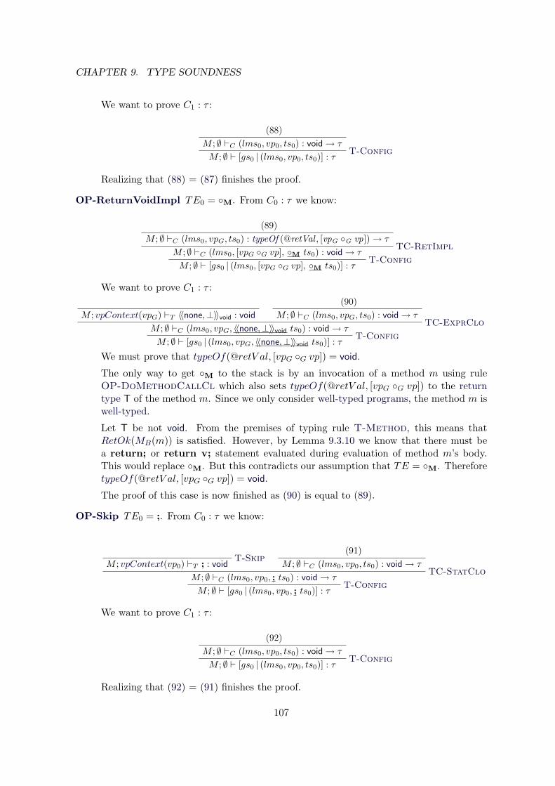
CHAPTER 9. TYPE SOUNDNESS

We want to prove C1 : τ :

(88)M ; ∅ `C (lms0, vp0, ts0) : void→ τ

T-ConfigM ; ∅ ` [gs0 | (lms0, vp0, ts0)] : τ

Realizing that (88) = (87) finishes the proof.

OP-ReturnVoidImpl TE0 = M. From C0 : τ we know:

(89)M ; ∅ `C (lms0, vpG, ts0) : typeOf (@retVal , [vpG G vp])→ τ

TC-RetImplM ; ∅ `C (lms0, [vpG G vp], M ts0) : void→ τ

T-ConfigM ; ∅ ` [gs0 | (lms0, [vpG G vp], M ts0)] : τ

We want to prove C1 : τ :

M ; vpContext(vpG) `T 〈〈none,⊥〉〉void : void

(90)M ; ∅ `C (lms0, vpG, ts0) : void→ τ

TC-ExprCloM ; ∅ `C (lms0, vpG, 〈〈none,⊥〉〉void ts0) : void→ τ

T-ConfigM ; ∅ ` [gs0 | (lms0, vpG, 〈〈none,⊥〉〉void ts0)] : τ

We must prove that typeOf(@retV al, [vpG G vp]) = void.

The only way to get M to the stack is by an invocation of a method m using ruleOP-DoMethodCallCl which also sets typeOf(@retV al, [vpG G vp]) to the returntype T of the method m. Since we only consider well-typed programs, the method m iswell-typed.

Let T be not void. From the premises of typing rule T-Method, this means thatRetOk(MB(m)) is satisfied. However, by Lemma 9.3.10 we know that there must bea return; or return v; statement evaluated during evaluation of method m’s body.This would replace M. But this contradicts our assumption that TE = M. ThereforetypeOf(@retV al, [vpG G vp]) = void.

The proof of this case is now finished as (90) is equal to (89).

OP-Skip TE0 = ;. From C0 : τ we know:

T-SkipM ; vpContext(vp0) `T ; : void

(91)M ; ∅ `C (lms0, vp0, ts0) : void→ τ

TC-StatCloM ; ∅ `C (lms0, vp0, ; ts0) : void→ τ

T-ConfigM ; ∅ ` [gs0 | (lms0, vp0, ; ts0)] : τ

We want to prove C1 : τ :

(92)M ; ∅ `C (lms0, vp0, ts0) : void→ τ

T-ConfigM ; ∅ ` [gs0 | (lms0, vp0, ts0)] : τ

Realizing that (92) = (91) finishes the proof.

107

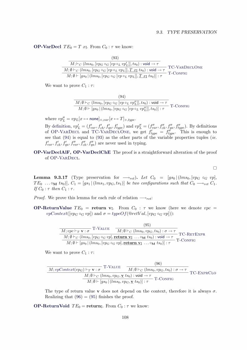
9.3. TYPE PRESERVATION

OP-VarDecl TE0 = T x;. From C0 : τ we know:

(93)M ;`C (lms0, [vpG G [vp L vp′

L]], ts0) : void→ τTC-VarDeclOne

M ; ∅ `C (lms0, [vpG G [vp L vpL]], T x; ts0) : void→ τT-Config

M ; ∅ ` [gs0 | (lms0, [vpG G [vp L vpL]], T x; ts0)] : τ

We want to prove C1 : τ :

(94)M ; ∅ `C (lms0, [vpG G [vp L vp′′

L]], ts0) : void→ τT-Config

M ; ∅ ` [gs0 | (lms0, [vpG G [vp L vp′′L]], ts0)] : τ

where vp′′L = vpL[x 7→ none]+,var[x 7→ T ]+,type.

By definition, vp′L = (f ′var, f′ch, f

′qa, f

′type) and vp′′L = (f ′′var, f

′′ch, f

′′qa, f

′′type). By definitions

of OP-VarDecl and TC-VarDeclOne, we get f ′type = f ′′type. This is enough tosee that (94) is equal to (93) as the other parts of the variable properties tuples (ie.f ′var, f

′ch, f

′qa, f

′′var, f

′′ch, f

′′qa) are never used in typing.

OP-VarDeclAlF, OP-VarDeclChE The proof is a straightforward alteration of the proofof OP-VarDecl.

Lemma 9.3.17 (Type preservation for −→ret). Let C0 = [gs0 | (lms0, [vpG G vp],TE0 . . . M ts0)], C1 = [gs1 | (lms1, vpG, ts1)] be two configurations such that C0 −→ret C1.If C0 : τ then C1 : τ .

Proof. We prove this lemma for each rule of relation −→ret:

OP-ReturnValue TE0 = return v;. From C0 : τ we know (here we denote vpc =vpContext([vpG G vp]) and σ = typeOf(@retV al, [vpG G vp])):

T-ValueM ; vpc `T v : σ

(95)M ; ∅ `C (lms0, vpG, ts0) : σ → τ

TC-RetExprM ; ∅ `C (lms0, [vpG G vp], return v; . . . M ts0) : void→ τ

T-ConfigM ; ∅ ` [gs0 | (lms0, [vpG G vp], return v; . . . M ts0)] : τ

We want to prove C1 : τ :

T-ValueM ; vpContext(vpG) `T v : σ

(96)M ; ∅ `C (lms0, vpG, ts0) : σ → τ

TC-ExprCloM ; ∅ `C (lms0, vpG,v ts0) : void→ τ

T-ConfigM ; ∅ ` [gs0 | (lms0, vpG,v ts0)] : τ

The type of return value v does not depend on the context, therefore it is always σ.Realizing that (96) = (95) finishes the proof.

OP-ReturnVoid TE0 = return;. From C0 : τ we know:

108

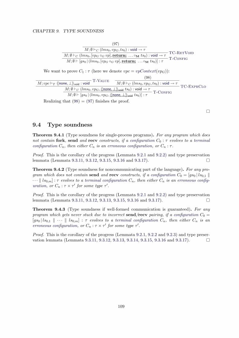
CHAPTER 9. TYPE SOUNDNESS

(97)M ; ∅ `C (lms0, vpG, ts0) : void→ τ

TC-RetVoidM ; ∅ `C (lms0, [vpG G vp], return; . . . M ts0) : void→ τ

T-ConfigM ; ∅ ` [gs0 | (lms0, [vpG G vp], return; . . . M ts0)] : τ

We want to prove C1 : τ (here we denote vpc = vpContext(vpG)):

T-ValueM ; vpc `T 〈〈none,⊥〉〉void : void

(98)M ; ∅ `C (lms0, vpG, ts0) : void→ τ

TC-ExprCloM ; ∅ `C (lms0, vpG, 〈〈none,⊥〉〉void ts0) : void→ τ

T-ConfigM ; ∅ ` [gs0 | (lms0, vpG, 〈〈none,⊥〉〉void ts0)] : τ

Realizing that (98) = (97) finishes the proof.

9.4 Type soundness

Theorem 9.4.1 (Type soundness for single-process programs). For any program which doesnot contain fork, send and recv constructs, if a configuration C0 : τ evolves to a terminalconfiguration Cn, then either Cn is an erroneous configuration, or Cn : τ .

Proof. This is the corollary of the progress (Lemmata 9.2.1 and 9.2.2) and type preservationlemmata (Lemmata 9.3.11, 9.3.12, 9.3.15, 9.3.16 and 9.3.17).

Theorem 9.4.2 (Type soundness for noncommunicating part of the language). For any pro-gram which does not contain send and recv constructs, if a configuration C0 = [gs0 | ls0,1 ‖· · · ‖ ls0,m] : τ evolves to a terminal configuration Cn, then either Cn is an erroneous config-uration, or Cn : τ × τ ′ for some type τ ′.

Proof. This is the corollary of the progress (Lemmata 9.2.1 and 9.2.2) and type preservationlemmata (Lemmata 9.3.11, 9.3.12, 9.3.13, 9.3.15, 9.3.16 and 9.3.17).

Theorem 9.4.3 (Type soundness if well-formed communication is guaranteed). For anyprogram which gets never stuck due to incorrect send/recv pairing, if a configuration C0 =[gs0 | ls0,1 ‖ · · · ‖ ls0,m] : τ evolves to a terminal configuration Cn, then either Cn is anerroneous configuration, or Cn : τ × τ ′ for some type τ ′.

Proof. This is the corollary of the progress (Lemmata 9.2.1, 9.2.2 and 9.2.3) and type preser-vation lemmata (Lemmata 9.3.11, 9.3.12, 9.3.13, 9.3.14, 9.3.15, 9.3.16 and 9.3.17).

109

9.4. TYPE SOUNDNESS

110

Chapter 10

Comparison with related work

In this chapter, we compare LanQ features with several other languages and process algebras.This comparison can be used as a simple key when LanQ is appropriate for desired usage andwhen another language should be better chosen.

We first briefly recall the properties of LanQ. The other formalisms will be presented in asimilar manner.

10.1 LanQ

Theoretical features:

• Category of the formalism: imperative language with several process-algebraic features

• Formal semantics: yes, operational

• Type soundness: yes

• Mixed or pure states: mixed

Practical features:

• Simulator implemented: yes, Java

LanQ is a complex language. It combines a programming language with several featuresof process algebras – process creation, interprocess communication. The comparison withseveral other existing formalisms follows.

10.2 Omer: QCL

Theoretical features:

• Category of the formalism: imperative language

• Formal semantics: no

• Type soundness: no

• Mixed or pure states: pure

Practical features:

111

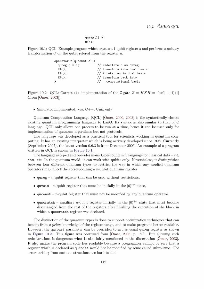
10.2. OMER: QCL

qureg[1] a;

U(a);

Figure 10.1: QCL: Example program which creates a 1-qubit register a and performs a unitarytransformation U on the qubit refered from the register a.

operator z(quconst c) qureg q = c; // redeclare c as quregH(q); // transform into dual basisX(q); // X-rotation in dual basisH(q); // transform back into

// computational basis

Figure 10.2: QCL: Correct (?) implementation of the Z-gate Z = HXH = |0〉〈0| − |1〉〈1|(from [Omer, 2003]).

• Simulator implemented: yes, C++, Unix only

Quantum Computation Language (QCL) [Omer, 2000, 2003] is the syntactically closestexisting quantum programming language to LanQ. Its syntax is also similar to that of Clanguage. QCL only allows one process to be run at a time, hence it can be used only forimplementation of quantum algorithms but not protocols.

The language was developed as a practical tool for scientists working in quantum com-puting. It has an existing interpreter which is being actively developed since 1998. Currently(September 2007), the latest version 0.6.3 is from December 2006. An example of a programwritten in QCL is shown in Figure 10.1.

The language is typed and provides many types found in C language for classical data – int,char, etc. In the quantum world, it can work with qubits only. Nevertheless, it distinguishesbetween four different quantum types to restrict the way in which any applied quantumoperators may affect the corresponding a n-qubit quantum register:

• qureg – n-qubit register that can be used without restrictions,

• quvoid – n-qubit register that must be initially in the |0〉⊗n state,

• quconst – n-qubit register that must not be modified by any quantum operator,

• quscratch – auxiliary n-qubit register initially in the |0〉⊗n state that must becomedisentangled from the rest of the registers after finishing the execution of the block inwhich a quscratch register was declared.

The distinction of the quantum types is done to support optimization techniques that canbenefit from a priori knowledge of the register usage, and to make programs better readable.However, the quconst parameter can be overriden to act as usual qureg register as shownin Figure 10.2. This figure was borrowed from [Omer, 2003, p. 80]. But allowing suchredeclarations is dangerous what is also fairly mentioned in the dissertation [Omer, 2003].It also makes the program code less readable because a programmer cannot be sure that aregister which is declared as quconst would not be modified by some called subroutine. Theerrors arising from such constructions are hard to find.

112

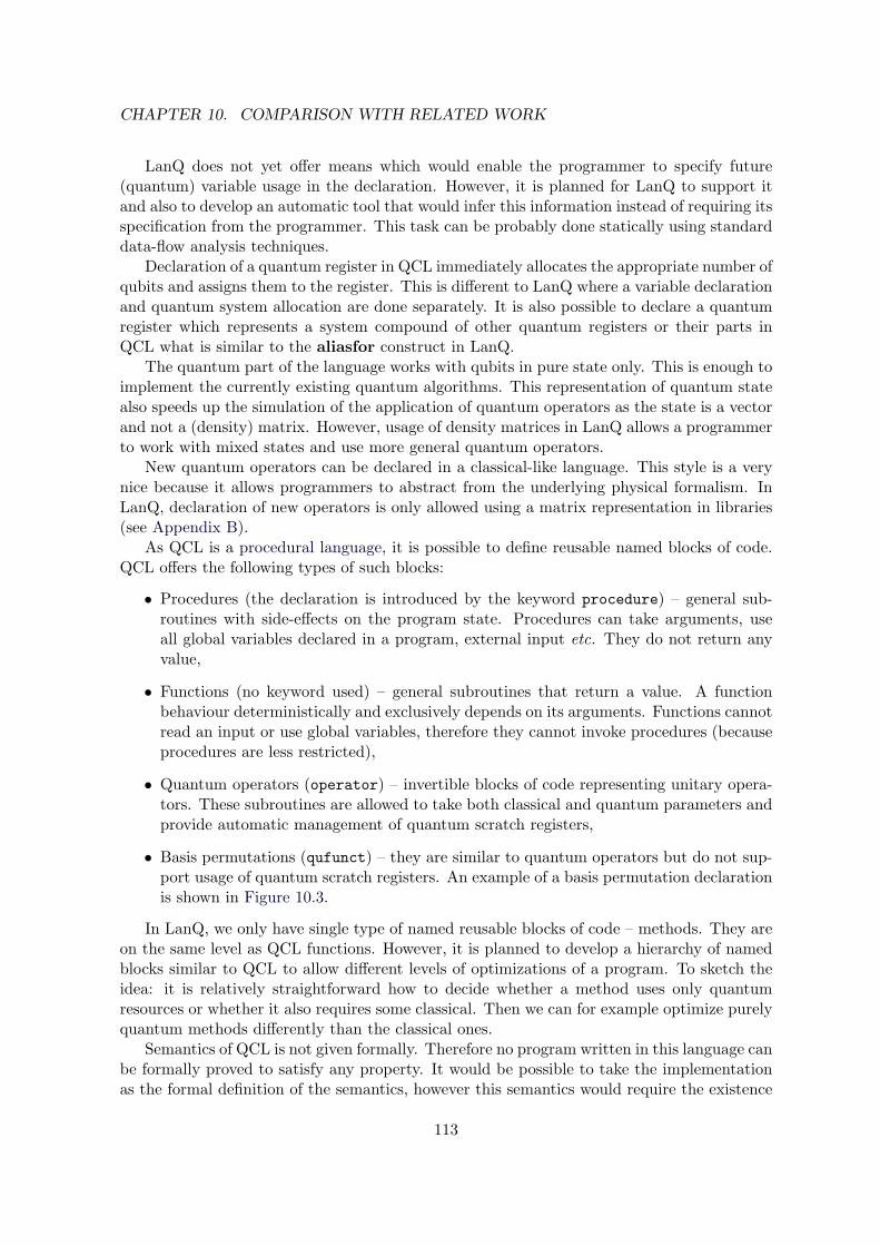
CHAPTER 10. COMPARISON WITH RELATED WORK

LanQ does not yet offer means which would enable the programmer to specify future(quantum) variable usage in the declaration. However, it is planned for LanQ to support itand also to develop an automatic tool that would infer this information instead of requiring itsspecification from the programmer. This task can be probably done statically using standarddata-flow analysis techniques.

Declaration of a quantum register in QCL immediately allocates the appropriate number ofqubits and assigns them to the register. This is different to LanQ where a variable declarationand quantum system allocation are done separately. It is also possible to declare a quantumregister which represents a system compound of other quantum registers or their parts inQCL what is similar to the aliasfor construct in LanQ.

The quantum part of the language works with qubits in pure state only. This is enough toimplement the currently existing quantum algorithms. This representation of quantum statealso speeds up the simulation of the application of quantum operators as the state is a vectorand not a (density) matrix. However, usage of density matrices in LanQ allows a programmerto work with mixed states and use more general quantum operators.

New quantum operators can be declared in a classical-like language. This style is a verynice because it allows programmers to abstract from the underlying physical formalism. InLanQ, declaration of new operators is only allowed using a matrix representation in libraries(see Appendix B).

As QCL is a procedural language, it is possible to define reusable named blocks of code.QCL offers the following types of such blocks:

• Procedures (the declaration is introduced by the keyword procedure) – general sub-routines with side-effects on the program state. Procedures can take arguments, useall global variables declared in a program, external input etc. They do not return anyvalue,

• Functions (no keyword used) – general subroutines that return a value. A functionbehaviour deterministically and exclusively depends on its arguments. Functions cannotread an input or use global variables, therefore they cannot invoke procedures (becauseprocedures are less restricted),

• Quantum operators (operator) – invertible blocks of code representing unitary opera-tors. These subroutines are allowed to take both classical and quantum parameters andprovide automatic management of quantum scratch registers,

• Basis permutations (qufunct) – they are similar to quantum operators but do not sup-port usage of quantum scratch registers. An example of a basis permutation declarationis shown in Figure 10.3.

In LanQ, we only have single type of named reusable blocks of code – methods. They areon the same level as QCL functions. However, it is planned to develop a hierarchy of namedblocks similar to QCL to allow different levels of optimizations of a program. To sketch theidea: it is relatively straightforward how to decide whether a method uses only quantumresources or whether it also requires some classical. Then we can for example optimize purelyquantum methods differently than the classical ones.

Semantics of QCL is not given formally. Therefore no program written in this language canbe formally proved to satisfy any property. It would be possible to take the implementationas the formal definition of the semantics, however this semantics would require the existence

113

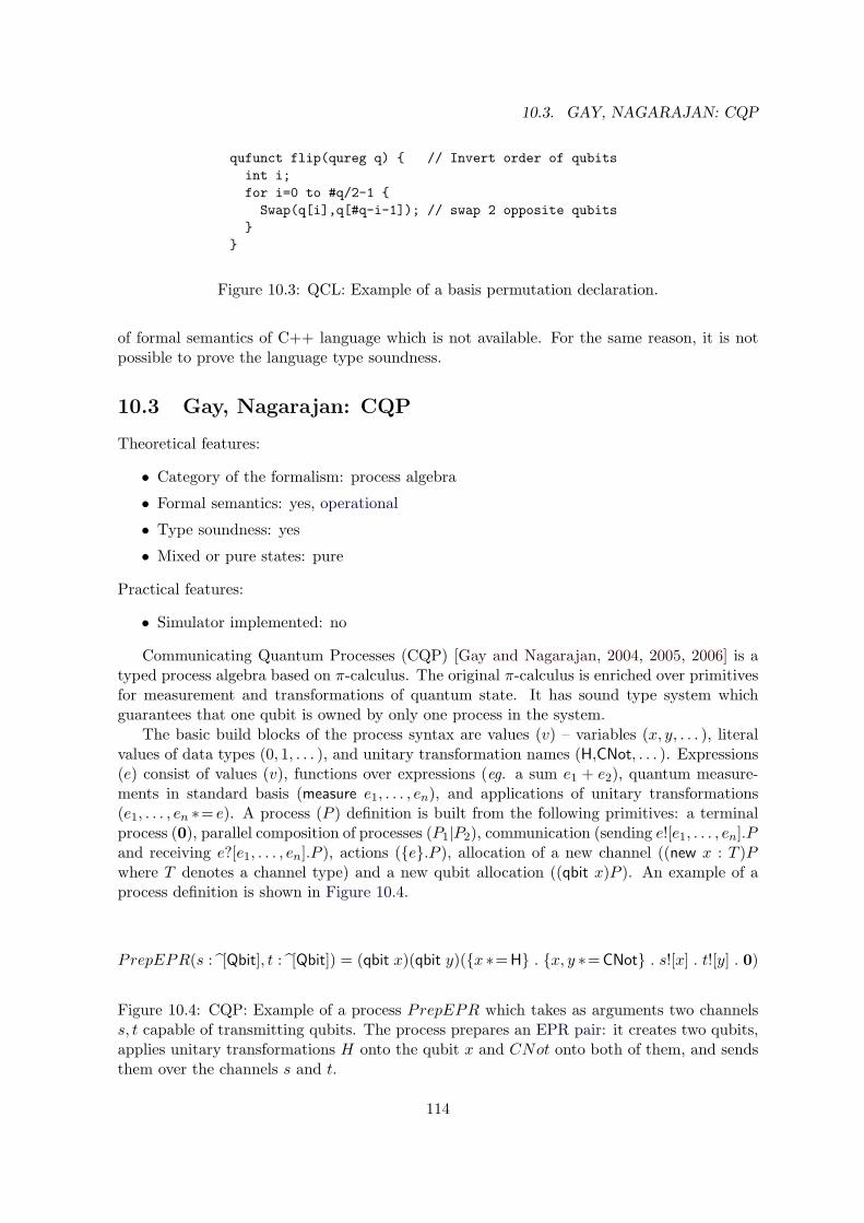
10.3. GAY, NAGARAJAN: CQP

qufunct flip(qureg q) // Invert order of qubitsint i;for i=0 to #q/2-1 Swap(q[i],q[#q-i-1]); // swap 2 opposite qubits

Figure 10.3: QCL: Example of a basis permutation declaration.

of formal semantics of C++ language which is not available. For the same reason, it is notpossible to prove the language type soundness.

10.3 Gay, Nagarajan: CQP

Theoretical features:

• Category of the formalism: process algebra

• Formal semantics: yes, operational

• Type soundness: yes

• Mixed or pure states: pure

Practical features:

• Simulator implemented: no

Communicating Quantum Processes (CQP) [Gay and Nagarajan, 2004, 2005, 2006] is atyped process algebra based on π-calculus. The original π-calculus is enriched over primitivesfor measurement and transformations of quantum state. It has sound type system whichguarantees that one qubit is owned by only one process in the system.

The basic build blocks of the process syntax are values (v) – variables (x, y, . . . ), literalvalues of data types (0, 1, . . . ), and unitary transformation names (H,CNot, . . . ). Expressions(e) consist of values (v), functions over expressions (eg. a sum e1 + e2), quantum measure-ments in standard basis (measure e1, . . . , en), and applications of unitary transformations(e1, . . . , en ∗= e). A process (P ) definition is built from the following primitives: a terminalprocess (0), parallel composition of processes (P1|P2), communication (sending e![e1, . . . , en].Pand receiving e?[e1, . . . , en].P ), actions (e.P ), allocation of a new channel ((new x : T )Pwhere T denotes a channel type) and a new qubit allocation ((qbit x)P ). An example of aprocess definition is shown in Figure 10.4.

PrepEPR(s : [Qbit], t : [Qbit]) = (qbit x)(qbit y)(x ∗=H . x, y ∗=CNot . s![x] . t![y] . 0)

Figure 10.4: CQP: Example of a process PrepEPR which takes as arguments two channelss, t capable of transmitting qubits. The process prepares an EPR pair: it creates two qubits,applies unitary transformations H onto the qubit x and CNot onto both of them, and sendsthem over the channels s and t.

114

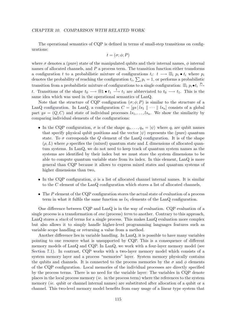
CHAPTER 10. COMPARISON WITH RELATED WORK

The operational semantics of CQP is defined in terms of small-step transitions on config-urations:

t = (σ;φ;P )

where σ denotes a (pure) state of the manipulated qubits and their internal names, φ internalnames of allocated channels, and P a process term. The transition function either transformsa configuration t to a probabilistic mixture of configurations ti: t −→ i pi • ti where pidenotes the probability of reaching the configuration ti,

∑i pi = 1, or performs a probabilistic

transition from a probabilistic mixture of configurations to a single configuration: i pi•tipi−→

t. Transitions of the shape t0 −→ 1 • t11−→ t1 are abbreviated to t0 −→ t1. This is the

same idea which was used in the operational semantics of LanQ.Note that the structure of CQP configuration (σ;φ;P ) is similar to the structure of a

LanQ configuration. In LanQ, a configuration C = [gs | ls1 ‖ · · · ‖ lsn] consists of a globalpart gs = (Q,C) and state of individual processes ls1, . . . , lsn. We show the similarity bycomparing individual elements of the configurations:

• In the CQP configuration, σ is of the shape q0, . . . , qn = |ψ〉 where qi are qubit namesthat specify physical qubit positions and the vector |ψ〉 represents the (pure) quantumstate. To σ corresponds the Q element of the LanQ configuration. It is of the shape(ρ, L) where ρ specifies the (mixed) quantum state and L dimensions of allocated quan-tum systems. In LanQ, we do not need to keep track of quantum system names as thesystems are identified by their index but we must store the system dimensions to beable to compute quantum variable state from its index. In this element, LanQ is moregeneral than CQP because it allows to express mixed states and quantum systems ofhigher dimensions than two,

• In the CQP configuration, φ is a list of allocated channel internal names. It is similarto the C element of the LanQ configuration which stores a list of allocated channels,

• The P element of the CQP configuration stores the actual state of evaluation of a processterm in what it fulfils the same function as lsi elements of the LanQ configuration.

One difference between CQP and LanQ is in the way of evaluation. CQP evaluation of asingle process is a transformation of one (process) term to another. Contrary to this approach,LanQ stores a stack of terms for a single process. This makes LanQ evaluation more complexbut also allows it to simply handle higher-level programming languages features such asvariable scope handling or returning a value from a method.

Another difference lies in variable handling. In LanQ, it is possible to have many variablespointing to one resource what is unsupported by CQP. This is a consequence of differentmemory models of LanQ and CQP. In LanQ, we work with a four-layer memory model (seeSection 7.1). In contrast, CQP works with a two-layer memory model which consists of asystem memory layer and a process “memories” layer. System memory physically containsthe qubits and channels. It is connected to the process memories by the σ and φ elementsof the CQP configuration. Local memories of the individual processes are directly specifiedby the process terms. There is no need for the variable layer: The variables in CQP denoteplaces in the local process memory (ie. in the process term) where the references to the systemmemory (ie. qubit or channel internal names) are substituted after allocation of a qubit or achannel. This two-level memory model benefits from easy usage of a linear type system that

115

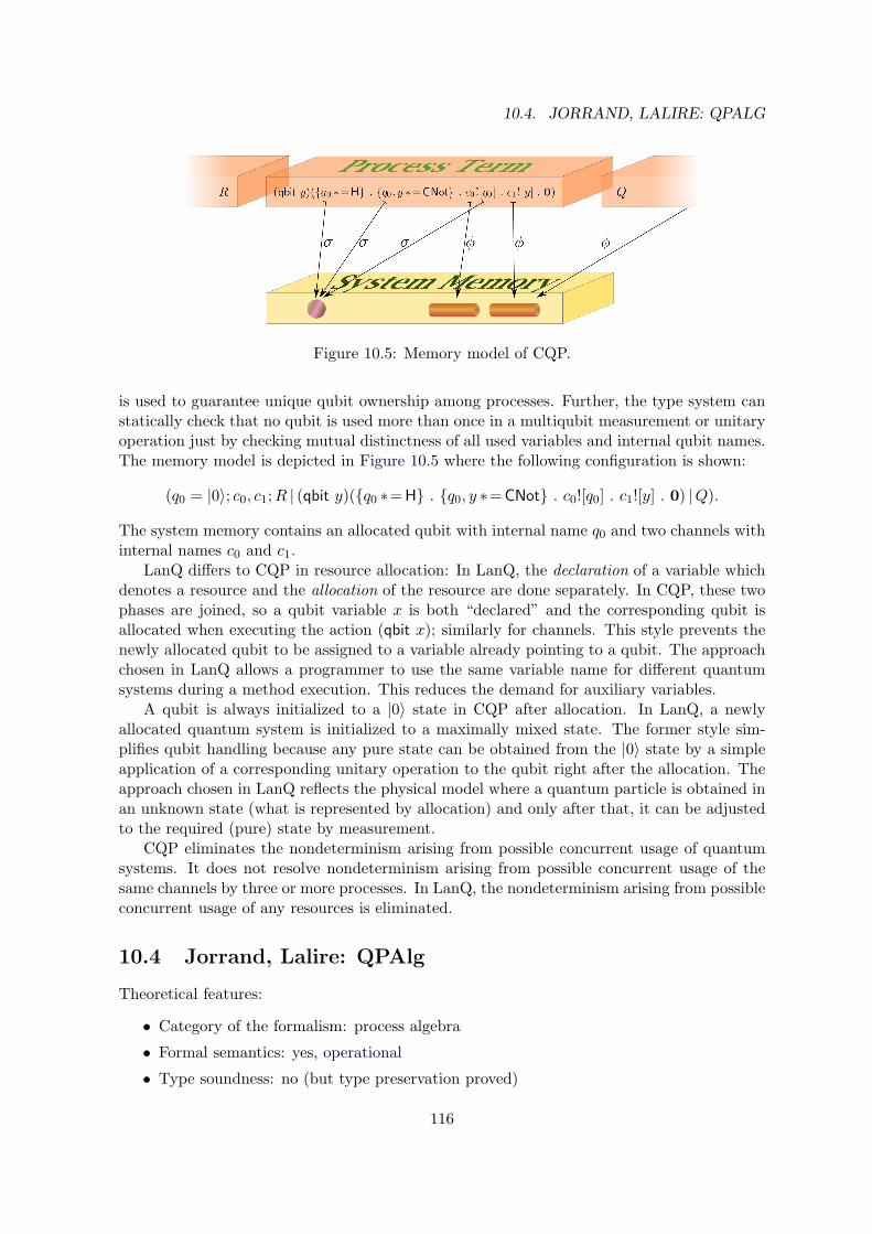
10.4. JORRAND, LALIRE: QPALG

Figure 10.5: Memory model of CQP.

is used to guarantee unique qubit ownership among processes. Further, the type system canstatically check that no qubit is used more than once in a multiqubit measurement or unitaryoperation just by checking mutual distinctness of all used variables and internal qubit names.The memory model is depicted in Figure 10.5 where the following configuration is shown:

(q0 = |0〉; c0, c1;R | (qbit y)(q0 ∗=H . q0, y ∗=CNot . c0![q0] . c1![y] . 0) |Q).

The system memory contains an allocated qubit with internal name q0 and two channels withinternal names c0 and c1.

LanQ differs to CQP in resource allocation: In LanQ, the declaration of a variable whichdenotes a resource and the allocation of the resource are done separately. In CQP, these twophases are joined, so a qubit variable x is both “declared” and the corresponding qubit isallocated when executing the action (qbit x); similarly for channels. This style prevents thenewly allocated qubit to be assigned to a variable already pointing to a qubit. The approachchosen in LanQ allows a programmer to use the same variable name for different quantumsystems during a method execution. This reduces the demand for auxiliary variables.

A qubit is always initialized to a |0〉 state in CQP after allocation. In LanQ, a newlyallocated quantum system is initialized to a maximally mixed state. The former style sim-plifies qubit handling because any pure state can be obtained from the |0〉 state by a simpleapplication of a corresponding unitary operation to the qubit right after the allocation. Theapproach chosen in LanQ reflects the physical model where a quantum particle is obtained inan unknown state (what is represented by allocation) and only after that, it can be adjustedto the required (pure) state by measurement.

CQP eliminates the nondeterminism arising from possible concurrent usage of quantumsystems. It does not resolve nondeterminism arising from possible concurrent usage of thesame channels by three or more processes. In LanQ, the nondeterminism arising from possibleconcurrent usage of any resources is eliminated.

10.4 Jorrand, Lalire: QPAlg

Theoretical features:

• Category of the formalism: process algebra

• Formal semantics: yes, operational

• Type soundness: no (but type preservation proved)

116

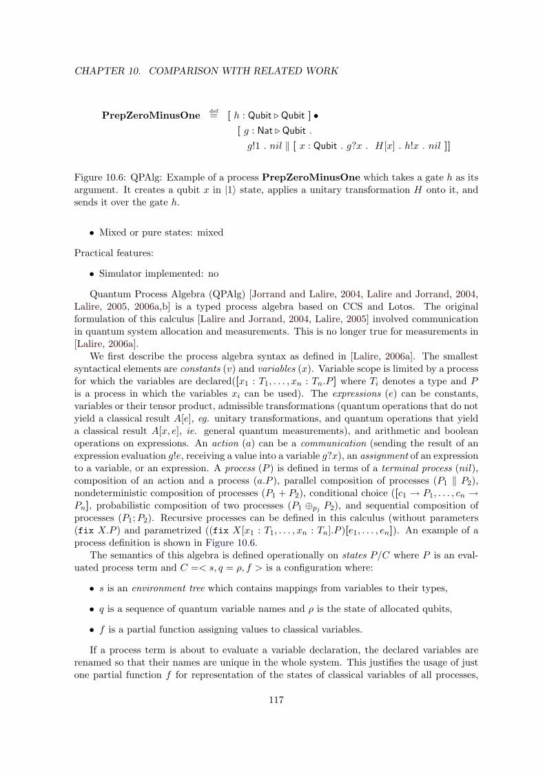
CHAPTER 10. COMPARISON WITH RELATED WORK

PrepZeroMinusOne def= [ h : Qubit . Qubit ] •[ g : Nat . Qubit .

g!1 . nil ‖ [ x : Qubit . g?x . H[x] . h!x . nil ]]

Figure 10.6: QPAlg: Example of a process PrepZeroMinusOne which takes a gate h as itsargument. It creates a qubit x in |1〉 state, applies a unitary transformation H onto it, andsends it over the gate h.

• Mixed or pure states: mixed

Practical features:

• Simulator implemented: no

Quantum Process Algebra (QPAlg) [Jorrand and Lalire, 2004, Lalire and Jorrand, 2004,Lalire, 2005, 2006a,b] is a typed process algebra based on CCS and Lotos. The originalformulation of this calculus [Lalire and Jorrand, 2004, Lalire, 2005] involved communicationin quantum system allocation and measurements. This is no longer true for measurements in[Lalire, 2006a].

We first describe the process algebra syntax as defined in [Lalire, 2006a]. The smallestsyntactical elements are constants (v) and variables (x). Variable scope is limited by a processfor which the variables are declared([x1 : T1, . . . , xn : Tn.P ] where Ti denotes a type and Pis a process in which the variables xi can be used). The expressions (e) can be constants,variables or their tensor product, admissible transformations (quantum operations that do notyield a classical result A[e], eg. unitary transformations, and quantum operations that yielda classical result A[x, e], ie. general quantum measurements), and arithmetic and booleanoperations on expressions. An action (a) can be a communication (sending the result of anexpression evaluation g!e, receiving a value into a variable g?x), an assignment of an expressionto a variable, or an expression. A process (P ) is defined in terms of a terminal process (nil),composition of an action and a process (a.P ), parallel composition of processes (P1 ‖ P2),nondeterministic composition of processes (P1 + P2), conditional choice ([c1 → P1, . . . , cn →Pn], probabilistic composition of two processes (P1 ⊕pj P2), and sequential composition ofprocesses (P1;P2). Recursive processes can be defined in this calculus (without parameters(fix X.P ) and parametrized ((fix X[x1 : T1, . . . , xn : Tn].P )[e1, . . . , en]). An example of aprocess definition is shown in Figure 10.6.

The semantics of this algebra is defined operationally on states P/C where P is an eval-uated process term and C =< s, q = ρ, f > is a configuration where:

• s is an environment tree which contains mappings from variables to their types,

• q is a sequence of quantum variable names and ρ is the state of allocated qubits,

• f is a partial function assigning values to classical variables.

If a process term is about to evaluate a variable declaration, the declared variables arerenamed so that their names are unique in the whole system. This justifies the usage of justone partial function f for representation of the states of classical variables of all processes,

117

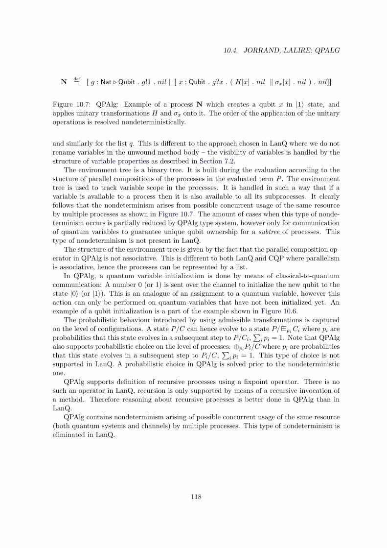
10.4. JORRAND, LALIRE: QPALG

N def= [ g : Nat . Qubit . g!1 . nil ‖ [ x : Qubit . g?x . ( H[x] . nil ‖ σx[x] . nil ) . nil]]

Figure 10.7: QPAlg: Example of a process N which creates a qubit x in |1〉 state, andapplies unitary transformations H and σx onto it. The order of the application of the unitaryoperations is resolved nondeterministically.

and similarly for the list q. This is different to the approach chosen in LanQ where we do notrename variables in the unwound method body – the visibility of variables is handled by thestructure of variable properties as described in Section 7.2.

The environment tree is a binary tree. It is built during the evaluation according to thestucture of parallel compositions of the processes in the evaluated term P . The environmenttree is used to track variable scope in the processes. It is handled in such a way that if avariable is available to a process then it is also available to all its subprocesses. It clearlyfollows that the nondeterminism arises from possible concurrent usage of the same resourceby multiple processes as shown in Figure 10.7. The amount of cases when this type of nonde-terminism occurs is partially reduced by QPAlg type system, however only for communicationof quantum variables to guarantee unique qubit ownership for a subtree of processes. Thistype of nondeterminism is not present in LanQ.

The structure of the environment tree is given by the fact that the parallel composition op-erator in QPAlg is not associative. This is different to both LanQ and CQP where parallelismis associative, hence the processes can be represented by a list.

In QPAlg, a quantum variable initialization is done by means of classical-to-quantumcommunication: A number 0 (or 1) is sent over the channel to initialize the new qubit to thestate |0〉 (or |1〉). This is an analogue of an assignment to a quantum variable, however thisaction can only be performed on quantum variables that have not been initialized yet. Anexample of a qubit initialization is a part of the example shown in Figure 10.6.

The probabilistic behaviour introduced by using admissible transformations is capturedon the level of configurations. A state P/C can hence evolve to a state P/pi Ci where pi areprobabilities that this state evolves in a subsequent step to P/Ci,

∑i pi = 1. Note that QPAlg

also supports probabilistic choice on the level of processes: ⊕piPi/C where pi are probabilitiesthat this state evolves in a subsequent step to Pi/C,

∑i pi = 1. This type of choice is not

supported in LanQ. A probabilistic choice in QPAlg is solved prior to the nondeterministicone.

QPAlg supports definition of recursive processes using a fixpoint operator. There is nosuch an operator in LanQ, recursion is only supported by means of a recursive invocation ofa method. Therefore reasoning about recursive processes is better done in QPAlg than inLanQ.

QPAlg contains nondeterminism arising of possible concurrent usage of the same resource(both quantum systems and channels) by multiple processes. This type of nondeterminism iseliminated in LanQ.

118

Chapter 11

Conclusion

We have developed an imperative typed quantum programming language LanQ that also hasseveral features of process algebras. It supports implementation of algorithms and multipartyprotocols that use both quantum and classical data. The statements manipulating quantumand classical data can be arbitrarily interleaved.

We have defined the language syntax which is similar to the syntax of C language, itsoperational semantics and its type system. We have proved language type soundness forthe restricted part of the language which does not contain send and recv statements, andfor the whole language provided the executed programs are guaranteed to use only a well-formed communication. This makes the language very usable for scientists who can use it forverification of properties of quantum algorithms and protocols.

We have shown that individual resources are guaranteed to be accesible to at most oneprocess at a time. This way we minimize nondeterminism – there is no nondeterminism inevolution of individual processes running in the system. The only nondeterminism arises fromthe choice of order of simultaneously running processes evolution. This feature significantlysimplifies the language implementation.

The language has existing simulator available from the address http://lanq.sf.net/.The existence of this implementation brings the language to the stage when it can be practi-cally used for implementation of quantum algorithms and protocols, and makes it a usable toolfor a machine-assisted formal verification of the properties of the algorithms and protocols.

There are several directions which the future research on LanQ can take, both theoreticallyand practically. We outline those most remarkable in the following paragraphs.

From the theoretical point of view, it would be nice to develop a notion of process equiv-alence for LanQ. It can be then used to develop optimization techniques for LanQ programs.

LanQ does not have denotational semantics yet. Creation of this type of semantics is ahard task. The semantics will be probably first developed for the single-process part of thelanguage. Then it will be probably developed for the restricted language without communi-cating capabilities. The latter semantics will surely benefit from the fact that the evolutionof individual processes is deterministic, the only nondeterminism arises from the possibilityof different order of evaluation of different processes.

From practical point of view, there are several improvements that should be done to makeLanQ more comfortable for its users. It would be convenient to allow programmers to definequantum operators in a classical-like language.

Simulator speed is currently painful. The main reason is the time complexity of manip-

119

ulation with density matrix that represents quantum state of allocated quantum systems.This can be solved by using several different implementations of quantum memory – oneusing mixed states, other using pure states, other for example stabilizer states, and possiblyin the future another one for a real quantum memory. The user could choose which of theimplementations he prefers for an execution of his program. This would indeed involve smallchanges in the semantics, at least for a quantum system allocation because the maximallymixed state is not be expressible in some of these formalisms.

The quantum systems that are not used remain in the system memory. Therefore weshould (theoretically) elaborate and (practically) implement a kind of garbage collector thatfrees inaccessible resources from the system memory.

120

References

S. Aaronson and D. Gottesman. Improved simulation of stabilizer circuits. Phys. Rev. A, 70(5), 2004.

S. Abramsky and B. Coecke. A categorical semantics of quantum protocols. quant-ph/0402130, 2004. URL http://www.arxiv.org/abs/quant-ph/0402130.

S. Abramsky and G. McCusker. Game semantics. In H. Schwichtenberg and U. Berger, editors,Computational Logic: Proceedings of the 1997 Marktoberdorf Summer School, pages 1–56.Springer-Verlag, 1999.

R. Alleaume, J. Bouda, C. Branciard, T. Debuisschert, M. Dianati, N. Gisin, M. Godfrey,P. Grangier, T. Langer, A. Leverrier, N. Lutkenhaus, P. Painchault, M. Peev, A. Poppe,T. Pornin, J. Rarity, R. Renner, G. Ribordy, M. Riguidel, L. Salvail, A. Shields, H. We-infurter, and A. Zeilinger. SECOQC White Paper on Quantum Key Distribution andCryptography. quant-ph/0701168, 2007. URL http://www.arxiv.org/abs/quant-ph/0701168.

T. Altenkirch and J. Grattage. A functional quantum programming language. quant-ph/0409065, 2004. URL http://www.arxiv.org/abs/quant-ph/0409065.

J. Baeten. A brief history of process algebra. Technical Report CSR 04-02, Vakgroep In-formatica, Technische Universiteit Eindhoven, 2004. URL http://www.win.tue.nl/fm/0402history.pdf.

J. C. M. Baeten and W. P. Weijland. Process algebra. Cambridge University Press, NewYork, NY, USA, 1990. ISBN 0-521-40043-0.

R. Baltazar, P. amd Chadha, P. Mateus, and A. Sernadas. Towards model-checking quantumsecurity protocols. In Dini, P., editor, Proceedings of the First Workshop on QuantumSecurity: QSec’07. IEEE Press, 2007.

C. Bennett and G. Brassard. Quantum Cryptography: Public Key Distribution and CoinTossing. In Proceedings of IEEE International Conference on Computers Systems andSignal Processing, pages 175–179, India, Dec. 1984. Bangalore.

C. H. Bennett and S. J. Wiesner. Communication via one- and two-particle operators oneinstein-podolsky-rosen states. Phys. Rev. Lett., 69(20):2881–2884, Nov 1992. doi: 10.1103/PhysRevLett.69.2881.

C. H. Bennett, G. Brassard, and N. D. Mermin. Quantum cryptography without Bell’stheorem. Phys. Rev. Lett., 68(5):557–559, 1992.

121

REFERENCES

C. H. Bennett, G. Brassard, C. Crepeau, R. Jozsa, A. Peres, and W. K. Wootters. Teleportingan unknown quantum state via dual classical and einstein-podolsky-rosen channels. Phys.Rev. Lett., 70(13):1895–1899, Mar 1993. doi: 10.1103/PhysRevLett.70.1895.

J. Bergstra and J. Klop. Process algebra for synchronous communication. Information andControl, 60(1/3):109–137, 1984.

J. A. Bergstra, A. Ponse, and S. A. Smolka, editors. Handbook of Process Algebra, New York,NY, USA, 2001. Elsevier Science Inc. ISBN 0444828303.

E. Bernstein and U. Vazirani. Quantum complexity theory. SIAM J. Comput., 26(5):1411–1473, 1997. URL http://citeseer.ist.psu.edu/bernstein97quantum.html.

S. Bettelli, T. Calarco, and L. Serafini. Toward an architecture for quantum programming,2001. URL http://www.arxiv.org/abs/cs.PL/0103009.

G. Bierman, M. Parkinson, and A. Pitts. MJ: An imperative core calculus for Java and Javawith effects. Technical Report 563, Cambridge University Computer Laboratory, April2003. URL citeseer.ist.psu.edu/article/bierman03mj.html.

L. Cardelli. Type systems. In A. B. Tucker, editor, The Computer Science and Engineer-ing Handbook. CRC Press, 2004. URL http://research.microsoft.com/Users/luca/Papers/TypeSystems.pdf.

D. Cazorla, F. Cuartero, V. V. Ruiz, F. L. Pelayo, and J. J. Pardo. Algebraic theory ofprobabilistic and nondeterministic processes. J. Log. Algebr. Program., 55(1-2):57–103,2003.

B. Coecke. Kindergarten Quantum Mechanics. quant-ph/0510032, 2005. URL http://www.arxiv.org/abs/quant-ph/0510032.

D. Deutsch. Quantum computational networks. Proceedings of the Royal Societyof London Ser. A, A425(1868):73–90, 1989. URL http://citeseer.ist.psu.edu/deutsch85quantum.html.

D. Deutsch. Quantum theory, the Church-Turing principle and the universal quantum com-puter. Proceedings of the Royal Society of London Ser. A, A400:97–117, 1985. URLhttp://citeseer.ist.psu.edu/deutsch85quantum.html.

D. Deutsch and R. Jozsa. Rapid Solution of Problems by Quantum Computation. In Pro-ceedings: Mathematical and Physical Sciences, volume 439, pages 553–558, 1992.

A. Einstein, B. Podolsky, and N. Rosen. Can quantum-mechanical description of physicalreality be considered complete? Phys. Rev., 47(10):777–780, May 1935. doi: 10.1103/PhysRev.47.777.

A. K. Ekert. Quantum cryptography based on bell’s theorem. Phys. Rev. Lett., 67(6):661–663,1991.

R. Feynman. The Feynman Lectures on Physics, The Definitive Edition Volume 3. Addison-Wesley, 2006. ISBN 0805390499.

122

REFERENCES

R. Feynman. Simulating Physics with Computers. International Journal of The-oretical Physics, 21(6&7):467–488, 1982. URL http://citeseer.ist.psu.edu/feynman82simulating.html.

W. Fokkink. Introduction to Process Algebra. Springer-Verlag New York, Inc., Secaucus, NJ,USA, 2000. ISBN 354066579X.

S. Gay and M. Hole. Subtyping for session types in the pi calculus. Acta Informatica, 42(2):191–225, 2005.

S. J. Gay. Quantum programming languages: Survey and bibliography. MathematicalStructures in Computer Science, 16(4), 2006. URL http://www.dcs.gla.ac.uk/~simon/publications/QPLsurvey.pdf.

S. J. Gay and R. Nagarajan. Communicating Quantum Processes. quant-ph/0409052, 2004.URL http://www.arxiv.org/abs/quant-ph/0409052.

S. J. Gay and R. Nagarajan. Communicating quantum processes. In POPL ’05: Proceedingsof the 32nd ACM Symposium on Principles of Programming Languages, pages 145–157,2005. ISBN 1-58113-830-X.

S. J. Gay and R. Nagarajan. Types and typechecking for Communicating Quantum Processes.Mathematical. Structures in Comp. Sci., 16:375–406, 2006. ISSN 0960-1295.

S. J. Gay, R. Nagarajan, and N. Papanikolaou. QMC: A Model Checker for Quantum Systems.quant-ph/0704.3705v2, 2007. URL http://www.arxiv.org/abs/quant-ph/0704.3705v2.

I. Glendinning. Quantum programming languages and tools, 2005. URL http://www.vcpc.univie.ac.at/~ian/hotlist/qc/programming.shtml. Online catalogue.

D. Gottesman. The heisenberg representation of quantum computers. quant-ph/9807006,1998. URL http://www.arxiv.org/abs/quant-ph/9807006.

J. Gruska. Foundations of Computing. International Thomson Publishing Computer Press,1997. ISBN 1-85032-243-0.

J. Gruska. Quantum Computing. McGraw-Hill, 1999. ISBN 0-07-709503-0.

C. A. R. Hoare. Communicating sequential processes. Commun. ACM, 26(1):100–106, 1983.ISSN 0001-0782. doi: http://doi.acm.org/10.1145/357980.358021.

P. Jorrand and M. Lalire. Toward a quantum process algebra. In CF ’04: Proceedings of the1st conference on Computing frontiers, pages 111–119, New York, NY, USA, 2004. ACMPress. ISBN 1-58113-741-9. doi: http://doi.acm.org/10.1145/977091.977108.

E. Knill. Conventions for quantum pseudocode. Technical Report LAUR-96-2724, Los AlamosNational Laboratory, 1996. URL http://citeseer.ist.psu.edu/knill96conventions.html.

D. E. Knuth. The Art of Computer Programming, Volumes 1-3. Addison Wesley Professional,1998. ISBN 0-201-48541-9.

123

REFERENCES

N. Kobayashi, B. C. Pierce, and D. N. Turner. Linearity and the Pi-Calculus. In POPL ’96:Proceedings of the 23rd ACM SIGPLAN-SIGACT symposium on Principles of programminglanguages, pages 358–371, New York, NY, USA, 1996. ACM Press. ISBN 0-89791-769-3.doi: http://doi.acm.org/10.1145/237721.237804.

A. Kondacs and J. Watrous. On the power of quantum finite state automata. In FOCS ’97:Proceedings of the 38th Annual Symposium on Foundations of Computer Science (FOCS’97), page 66, Washington, DC, USA, 1997. IEEE Computer Society. ISBN 0-8186-8197-7.

M. Lalire. A Probabilistic Branching Bisimulation for Quantum Processes. quant-ph/0508116,2005. URL http://www.arxiv.org/abs/quant-ph/0508116.

M. Lalire. Developpement d’une notation alorithmique pour le calcul quantique. PhD thesis,Grenoble Institute of Technology, 2006a.

M. Lalire. Relations among Quantum Processes: Bisimilarity and Congruence. Mathematical.Structures in Comp. Sci., 16(3), 2006b. ISSN 0960-1295.

M. Lalire and P. Jorrand. A process-algebraic approach to concurrent and distributedquantum computation: operational semantics. quant-ph/0407005, 2004. URL http://www.arxiv.org/abs/quant-ph/0407005.

M. Lampis, K. G. Ginis, and N. S. Papaspyrou. Quantum data and control made easier. InP. Selinger, editor, Preliminary Proceedings of the 4th International Workshop on Quan-tum Programming Languages, pages 73–86, 2006. The final version will be published inElectronic Notes in Theoretical Computer Science.

D. W. Leung. Quantum computation by measurements. International Journal of QuantumInformation, 2(1):33–34, 2004.

D. Mayers. Quantum key distribution and string oblivious transfer in noisy channels. InCRYPTO ’96: Proceedings of the 16th Annual International Cryptology Conference onAdvances in Cryptology, pages 343–357, London, UK, 1996. Springer-Verlag. ISBN 3-540-61512-1.

J. McCarthy. A Basis for a Mathematical Theory of Computation. In P. Braffort andD. Hirschberg, editors, Computer Programming and Formal Systems, pages 33–70. North-Holland, Amsterdam, 1963. URL http://citeseer.ist.psu.edu/mccarthy63basis.html.

R. Milner. A theory of type polymorphism in programming. Journal of Computer and SystemSciences, 17:348–375, 1978.

R. Milner. A calculus of communicating systems, volume 92. Springer Verlag, 1980. ISBN0-387-10235-3.

R. Milner, J. Parrow, and D. Walker. A calculus of mobile processes, i. Inf. Comput., 100(1):1–40, 1992. ISSN 0890-5401. doi: http://dx.doi.org/10.1016/0890-5401(92)90008-4.

H. Mlnarık. LanQ – an Imperative Quantum Programming Language. In MEMICS 2006,2nd Doctoral Workshop on Mathematical and Engineering Methods in Computer Science,

124

REFERENCES

pages 113–120. Faculty of Information Technology, Brno University of Technology, 2006,Oct. 2006a. ISBN 80-214-3287-X.

H. Mlnarık. Operational Semantics of Quantum Programming Language LanQ. TechnicalReport FIMU-RS-2006-10, Faculty of Informatics, Masaryk University, 2006, Dec. 2006b.

H. Mlnarık. Operational Semantics and Type Soundness of Quantum Programming LanguageLanQ. quant-ph/0708.0890, 2007. URL http://arxiv.org/abs/0708.0890.

G. E. Moore. Cramming more components onto integrated circuits. Electronics, 38(8), April1965.

M. Nielsen and I. Chuang. Quantum computation and quantum information. CambridgeUniversity Press, 2000.

M. A. Nielsen. Universal quantum computation using only projective measurement, quantummemory, and preparation of the |0〉 state. Phys. Lett. A, 308(2-3):96–100, 2003.

B. Omer. Quantum programming in QCL. Master’s thesis, TU Vienna, 2000.

B. Omer. Structured Quantum Programming. PhD thesis, TU Vienna, 2003. URL http://tph.tuwien.ac.at/~oemer/doc/structquprog.ps.

C. Palamidessi. Comparing the expressive power of the synchronous and the asynchronousπ-calculus. In POPL ’97: Proceedings of the 24th ACM SIGPLAN-SIGACT symposiumon Principles of programming languages, pages 256–265, New York, NY, USA, 1997. ACMPress. ISBN 0-89791-853-3. doi: http://doi.acm.org/10.1145/263699.263731.

S. Perdrix. State transfer instead of teleportation in measurement-based quantum computa-tion. International Journal of Quantum Information, 3(1):219–223, 2005.

A. Peres. Quantum Theory: Concepts and Methods. Kluwer, 1995. ISBN 978-0-7923-3632-7.

J. Preskill. Lecture notes on physics 219/computer science 219 course, quantum computation,2000. Available at http://www.theory.caltech.edu/people/preskill/ph219/.

R. Raussendorf and H. J. Briegel. A one-way quantum computer. Phys. Rev. Lett., 86(22):5188–5191, May 2001. doi: 10.1103/PhysRevLett.86.5188.

J. W. Sanders and P. Zuliani. Quantum programming. In MPC, volume 1837 of LectureNotes in Computer Science, pages 80–99. Springer, 2000. ISBN 3-540-67727-5.

D. Scott and C. Strachey. Towards a mathematical semantics for computer languages.In J. Fox, editor, Proceedings Symposium Computers and Automata, pages 19–46.Polytechnic Institute of Brooklyn Press, 1971. URL http://citeseer.ist.psu.edu/mccarthy63basis.html.

P. Selinger. Towards a quantum programming language. Mathematical. Structures inComp. Sci., 14(4):527–586, 2004. ISSN 0960-1295. doi: http://dx.doi.org/10.1017/S0960129504004256.

125

REFERENCES

P. Selinger. Dagger compact closed categories and completely positive maps. In P. Selinger,editor, Preliminary Proceedings of the 3rd International Workshop on Quantum Program-ming Languages, pages 127–148, 2005. The final version will be published in ElectronicNotes in Theoretical Computer Science.

P. Selinger and B. Valiron. A lambda calculus for quantum computation with classical control.Mathematical. Structures in Comp. Sci., 16(3):527–552, 2006. ISSN 0960-1295. doi: http://dx.doi.org/10.1017/S0960129506005238.

P. W. Shor. Algorithms for quantum computation: Discrete logarithms and factoring. InProceedings of the 35th Annual Symposium on Foundations of Computer Science. IEEEComputer Society Press, 1994.

M. Sipser. Introduction to the Theory of Computation, Second Edition. Course Technology,2005. ISBN 978-0534950972.

K. Slonneger and B. L. Kurtz. Formal syntax and semantics of programming languages: alaboratory based approach. Addison-Wesley, 1995. ISBN 0-201-65697-3.

A. van Tonder. A Lambda Calculus for Quantum Computation. quant-ph/0307150, 2003a.URL http://www.arxiv.org/abs/quant-ph/0307150.

A. van Tonder. Quantum computation, categorical semantics and linear logic. quant-ph/0312174, 2003b. URL http://www.arxiv.org/abs/quant-ph/0312174.

J. Watrous. On One-Dimensional Quantum Cellular Automata. In IEEE Symposium onFoundations of Computer Science, pages 528–537, 1995. URL http://citeseer.ist.psu.edu/watrous95onedimensional.html.

W. Wootters and W. Zurek. A single quantum cannot be cloned. Nature, 299:802–803, 1982.

A. K. Wright and M. Felleisen. A syntactic approach to type soundness. Information and Com-putation, 115(1):38–94, 1994. URL http://citeseer.ist.psu.edu/wright92syntactic.html.

N. Yoshida and V. T. Vasconcelos. Language primitives and type discipline for structuredcommunication-based programming revisited: Two systems for higher-order session com-munication. Electron. Notes Theor. Comput. Sci., 171(4):73–93, 2007. ISSN 1571-0661.doi: http://dx.doi.org/10.1016/j.entcs.2007.02.056.

P. Zuliani. Quantum Programming. PhD thesis, University of Oxford, 2001. URL http://web.comlab.ox.ac.uk/oucl/work/paolo.zuliani/pzthesis.ps.gz.

126

Index

S-list, 45

accessible resourcechannel, 80channel end, 79quantum, 77

aliased quantum variable, 60aliasSubsyst, 57aliasSubsystL, 57argument types, 40

basis, 5computational, 5diagonal, 6Hadamard, 6standard, 5

basis vectors, 5BFOk, 88BFOk0, 90BFOki, 90blacksquare, 47block-forming statements, 35blocks, 35bra-ket notation, 6

categorical semantics, 15chanEnds, 57chanEndsL, 57channel type, 39closed expression, 37closed statement, 37closed term, 37CNOT, 10coalesce of g and f , 48communication

asynchronous, 18synchronous, 18

configuration, 54configuration syntax, 36

denotational semantics, 14density matrix, 8density operator, 8

reduced, 10dual basis, 6

empty variable properties tuple, 56entanglement, 10EPR pair, 10EPR state, 10erroneous configuration, 65ExpOk, 88ExpOk0, 90ExpOki, 90

fassignQAlias, 63fassignQSystemDirect, 61fassignQSystemInAlias, 61fassignQSystem, 62finite-dimensional Hilbert space, 5first-order, 15function lms, 55

g ∗ f , 48global reference, 50ground type, 39

Hadamard transformation, 7hermitian matrix, 8higher-order, 15Hilbert space, 5hole, 37

internal value, 63

layerstructured reference, 50system memory, 50value, 50variable, 50

127

INDEX

linearize, 46linearizebot, 46list length, 45list of lists of partial function tuples, 47list of partial function tuples, 47LMS, 55LMSQ, 55lmsQ, 55LMSChE , 55lmsChE , 55LMSCh, 55lmsCh, 55LMSCl, 55lmsCl, 55local, 49local memory state, 55local memory state update, 60local operations, 10local process configuration, 55local process memory, 49local reference, 50localAliasedV ars, 62

matrixdensity, 8hermitian, 8positive, 8trace, 8

maximally mixed state, 9measurement

projective, 7von Neumann, 7

memory reference, 51method, 33method body, 35method declaration, 33method header, 35method type, 40method typing context, 40mixed configuration, 56mixed state, 8

Names, 48

observable, 8operational semantics, 14operator

completely positive, 11

positive, 11trace-preserving, 11

paradigmfunctional, 15imperative, 15logical, 15

partial function tuple, 47partial trace, 10Pauli matrices, 7positive matrix, 8probability amplitudes, 6procedural language, 15program, 33projective measurement, 7projector, 7proper quantum variable, 60pure state, 6

quantum type, 39qubit, 5

recursive S-list, 45reduced density operator, 10Ref , 51RefG, 51RefL, 50RefQ, 50RefChE , 50RefCh, 50RefCl, 50RefGCh, 50RefGQ, 50Refnd, 51replacement, 46

list of partial function tuples, 47RetOk, 42return type, 40RTErr, 37rule

NP-Cong, 66NP-ProbEvol, 66NP-PropagProb, 66OP-AllocC, 67OP-AllocQ, 67OP-AssignExpr, 69OP-AssignNewValue, 69OP-AssignQAValueBad, 69

128

INDEX

OP-AssignQAValue, 69OP-AssignQValue, 69OP-AssignValue, 70OP-BlockEnd, 70OP-BlockHead, 66OP-Block, 70OP-Bracket, 66OP-DoFork, 73OP-DoMeasure, 75OP-DoMethodCallCl, 71OP-DoMethodCallQ, 72OP-ForkExpr, 73OP-IfExpr, 70OP-IfFalse, 70OP-IfTrue, 70OP-MeasureExpr, 74OP-MeasureOverlap, 74OP-MeasureUninit, 74OP-MethodCallExpr, 71OP-MethodCallQOverlap, 72OP-MethodCallQUninit, 72OP-PromoExpr, 67OP-PromoForget, 67OP-RecvExpr, 76OP-RecvUninit, 76OP-ReturnExpr, 73OP-ReturnValue, 73OP-ReturnVoidImpl, 73OP-ReturnVoid, 72OP-SendExpr1, 75OP-SendExpr2, 75OP-SendUninit, 75OP-Skip, 66OP-SubstE, 67OP-SubstS, 67OP-VarDeclAlF, 68OP-VarDeclMulti, 68OP-VarDecl, 68OP-Var, 66OP-While, 70SC-Assoc, 65SC-Comm, 65SC-Nil, 65

runtime error, 64ISQV, 65OQV, 64UV, 64

semantics, 14categorical, 15denotational, 14operational, 14

spectral decomposition, 8square, 47starting configuration, 65StkEl, 37StkRetOk, 89strong type soundness, 16stuck, 64superoperator, 11syntax, 14

block-forming elementary statement, 35block-forming statement, 35constant, 35expression, 35identifier, 35lists, 35number, 35promotable expression, 35recursive list, 35reference, 35runtime error, 37statement, 35term stack element, 37type, 35value, 35variable declaration, 35

system memory, 49

tensor product, 9term stack, 56terminal configuration, 65trace, 8type

bool, 39channel, 39channel end, 39compound system, 39int, 39MeasurementBasis, 39qdit, 39qbit, 39qtrit, 39Ref, 51RTErr, 39

129

INDEX

void, 39typeOf , 57Types, 40typing context, 40

unique channel end ownership property, 79unique channel ownership property, 80unique quantum system ownership prop-

erty, 78unitary, 6unmapQ, 58unmapChE , 59unmapCh, 59unmapnd, 58update, 46

list of partial function tuples, 47

V alues, 40variable declarations, 35variable properties, 55variable properties tuple, 56variable typing context, 40V arProp, 56V arPropL, 56varRef , 57varRefL, 57vector

bra, 6ket, 6orthogonal, 5orthonormal, 5

vector spacebasis, 5complete, 5

von Neumann measurement, 7vpContext, 84

weak type soundness, 16well-typed configuration, 83well-typed method, 43well-typed program, 40

130

Part III

Appendix

131

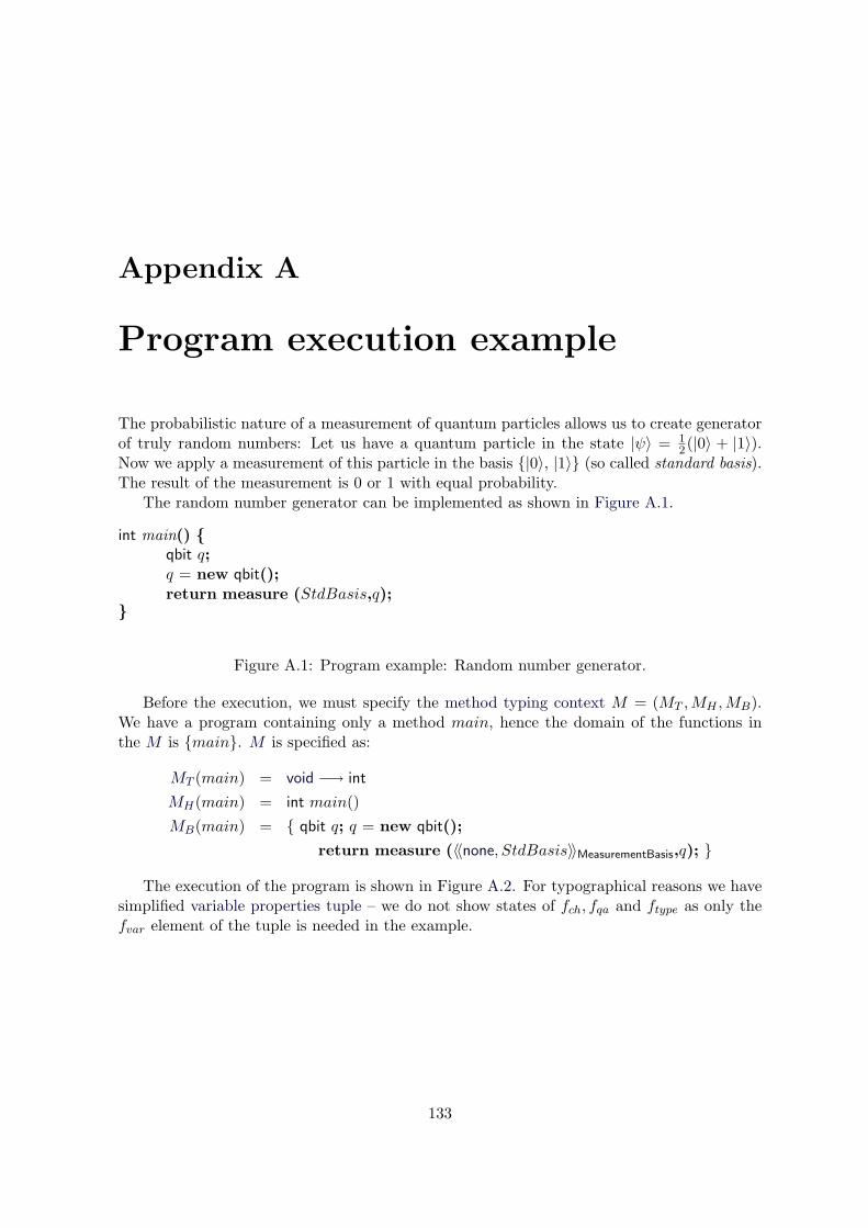
Appendix A

Program execution example

The probabilistic nature of a measurement of quantum particles allows us to create generatorof truly random numbers: Let us have a quantum particle in the state |ψ〉 = 1

2(|0〉 + |1〉).Now we apply a measurement of this particle in the basis |0〉, |1〉 (so called standard basis).The result of the measurement is 0 or 1 with equal probability.

The random number generator can be implemented as shown in Figure A.1.

int main() qbit q;q = new qbit();return measure (StdBasis,q);

Figure A.1: Program example: Random number generator.

Before the execution, we must specify the method typing context M = (MT ,MH ,MB).We have a program containing only a method main, hence the domain of the functions inthe M is main. M is specified as:

MT (main) = void −→ int

MH(main) = int main()MB(main) = qbit q; q = new qbit();

return measure (〈〈none, StdBasis〉〉MeasurementBasis,q);

The execution of the program is shown in Figure A.2. For typographical reasons we havesimplified variable properties tuple – we do not show states of fch, fqa and ftype as only thefvar element of the tuple is needed in the example.

133

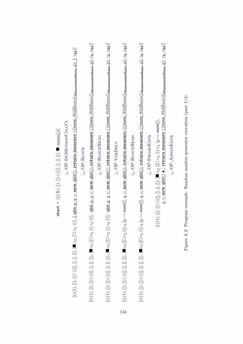
star

t=

[(((

1),[

]),[

])|(

([],

[],[],

[]),,m

ain

())]

↓ eO

P-D

oM

ethodC

allC

l

[(((

1),[

]),[

])|(

([],

[],[],

[]),[

G

[ L

♦]],

qbitq;q

=new

qbit()

;re

turn

mea

sure

(〈〈non

e,StdBasis〉〉 M

easu

rem

entB

asis,q)

; M

)]

↓ sO

P-B

lock

[(((

1),[

]),[

])|(

([],

[],[],

[]),[

G

[[ L

♦]L

♦]],

qbitq;q

=new

qbit()

;re

turn

mea

sure

(〈〈non

e,StdBasis〉〉 M

easu

rem

entB

asis,q)

;L M

)]

↓ rO

P-B

lockH

ead

[(((

1),[

]),[

])|(

([],

[],[],

[]),[

G

[[ L

♦]L

♦]],

qbitq;q

=new

qbit()

;re

turn

mea

sure

(〈〈non

e,StdBasis〉〉 M

easu

rem

entB

asis,q)

;L M

)]

↓ sO

P-V

arD

ecl

[(((

1),[

]),[

])|(

([],

[],[],

[]),[

G

[[ L

♦]L[q7→

non

e]]],q

=new

qbit()

;re

turn

mea

sure

(〈〈non

e,StdBasis〉〉 M

easu

rem

entB

asis,q)

;L M

)]

↓ rO

P-B

lockH

ead

[(((

1),[

]),[

])|(

([],

[],[],

[]),[

G

[[ L

♦]L[q7→

non

e]]],q

=new

qbit()

;re

turn

mea

sure

(〈〈non

e,StdBasis〉〉 M

easu

rem

entB

asis,q)

;L M

)]

↓ eO

P-P

romoExpr

[(((

1),[

]),[

])|(

([],

[],[],

[]),[

G

[[ L

♦]L

[q7→

non

e]]],

q=

new

qbit()•

;re

turn

mea

sure

(〈〈non

e,StdBasis〉〉 M

easu

rem

entB

asis,q)

; L M

)]

↓ eO

P-A

ssig

nExpr

Fig

ure

A.2

:P

rogr

amex

ampl

e:R

ando

mnu

mbe

rge

nera

tor

exec

utio

n(p

art

1/4)

.

134

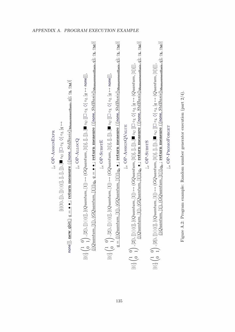
APPENDIX A. PROGRAM EXECUTION EXAMPLE

↓ eO

P-A

ssig

nExpr

[(((

1),[

]),[

])|(

([],

[],[],

[]),[

G

[[ L

♦]L

[q7→

non

e]]],

new

qbit()q

=••

;re

turn

mea

sure

(〈〈non

e,StdBasis〉〉 M

easu

rem

entB

asis,q)

; L M

)]

↓ vO

P-A

llocQ

[((1 2

( 10

01) ,[

2]),

[])|(

([],

[(Quantum,[

1])7→

(GQuantum,[

1])],[

],[]),[

G

[[ L

♦]L

[q7→

non

e]]],

〈〈(Quantum,[

1]),

(GQuantum,[

1])〉〉

Q2q

=••

;re

turn

mea

sure

(〈〈non

e,StdBasis〉〉 M

easu

rem

entB

asis,q)

; L M

)]

↓ eO

P-S

ubst

E

[((1 2

( 10

01) ,[

2]),

[])|(

([],

[(Quantum,[

1])7→

(GQuantum,[

1])],[

],[]),[

G

[[ L

♦]L

[q7→

non

e]]],

q=〈〈(Quantum,[

1]),

(GQuantum,[

1])〉〉

Q2•

;re

turn

mea

sure

(〈〈non

e,StdBasis〉〉 M

easu

rem

entB

asis,q)

; L M

)]

↓ vO

P-A

ssig

nQ

Value

[((1 2

( 10

01) ,[

2]),

[])|(

([],

[(Quantum,[

1])7→

(GQuantum,[

1])],[

],[]),[

G

[[ L

♦]L

[q7→

(Quantum,[

1])]

]],〈〈(Quantum,[

1]),

(GQuantum,[

1])〉〉

Q2•

;re

turn

mea

sure

(〈〈non

e,StdBasis〉〉 M

easu

rem

entB

asis,q)

; L M

)]

↓ eO

P-S

ubst

S

[((1 2

( 10

01) ,[

2]),

[])|(

([],

[(Quantum,[

1])7→

(GQuantum,[

1])],[

],[]),[

G

[[ L

♦]L

[q7→

(Quantum,[

1])]

]],〈〈(Quantum,[

1]),

(GQuantum,[

1])〉〉

Q2

;re

turn

mea

sure

(〈〈non

e,StdBasis〉〉 M

easu

rem

entB

asis,q)

; L M

)]

↓ sO

P-P

romoForget

Fig

ure

A.2

:P

rogr

amex

ampl

e:R

ando

mnu

mbe

rge

nera

tor

exec

utio

n(p

art

2/4)

.

135

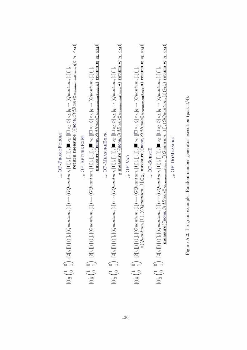
↓ sO

P-P

romoForget

[((1 2

( 10

01) ,[

2]),

[])|(

([],

[(Quantum,[

1])7→

(GQuantum,[

1])],[

],[]),[

G

[[ L

♦]L

[q7→

(Quantum,[

1])]

]],re

turn

mea

sure

(〈〈non

e,StdBasis〉〉 M

easu

rem

entB

asis,q)

; L M

)]

↓ eO

P-R

eturnExpr

[((1 2

( 10

01) ,[

2]),

[])|(

([],

[(Quantum,[

1])7→

(GQuantum,[

1])],[

],[]),[

G

[[ L

♦]L

[q7→

(Quantum,[

1])]

]],m

easu

re(〈〈

non

e,StdBasis〉〉 M

easu

rem

entB

asis,q)

retu

rn•; L M

)]

↓ eO

P-M

easu

reExpr

[((1 2

( 10

01) ,[

2]),

[])|(

([],

[(Quantum,[

1])7→

(GQuantum,[

1])],[

],[]),[

G

[[ L

♦]L

[q7→

(Quantum,[

1])]

]],q

mea

sure

(〈〈non

e,StdBasis〉〉 M

easu

rem

entB

asis,•)

retu

rn•; L M

)]

↓ vO

P-V

ar

[((1 2

( 10

01) ,[

2]),

[])|(

([],

[(Quantum,[

1])7→

(GQuantum,[

1])],[

],[]),[

G

[[ L

♦]L

[q7→

(Quantum,[

1])]

]],〈〈(Quantum,[

1]),

(GQuantum,[

1])〉〉

Q2m

easu

re(〈〈

non

e,StdBasis〉〉 M

easu

rem

entB

asis,•)

retu

rn•; L M

)]

↓ eO

P-S

ubst

E

[((1 2

( 10

01) ,[

2]),

[])|(

([],

[(Quantum,[

1])7→

(GQuantum,[

1])],[

],[]),[

G

[[ L

♦]L

[q7→

(Quantum,[

1])]

]],m

easu

re(〈〈

non

e,StdBasis〉〉 M

easu

rem

entB

asis,〈〈(Quantum,[

1]),

(GQuantum,[

1])〉〉

Q2)re

turn•; L M

)]

↓ vO

P-D

oM

easu

re

Fig

ure

A.2

:P

rogr

amex

ampl

e:R

ando

mnu

mbe

rge

nera

tor

exec

utio

n(p

art

3/4)

.

136

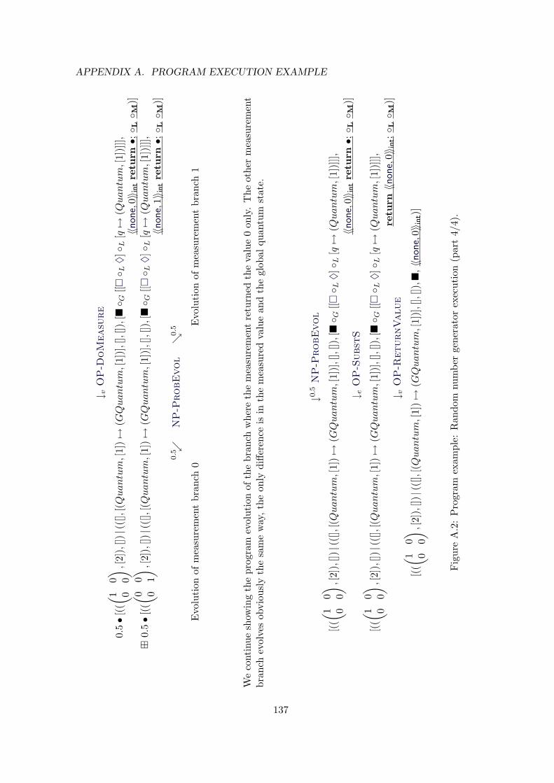
APPENDIX A. PROGRAM EXECUTION EXAMPLE

↓ vO

P-D

oM

easu

re

0.5•

[((( 1

00

0) ,[2]

),[])|(

([],

[(Quantum,[

1])7→

(GQuantum,[

1])],[

],[]),[

G

[[ L

♦]L

[q7→

(Quantum,[

1])]

]],〈〈n

one,

0〉〉 in

tre

turn•; L M

)]

0.5•

[((( 0

00

1) ,[2]

),[])|(

([],

[(Quantum,[

1])7→

(GQuantum,[

1])],[

],[]),[

G

[[ L

♦]L

[q7→

(Quantum,[

1])]

]],〈〈n

one,

1〉〉 in

tre

turn•; L M

)]0.5

NP-P

robEvol

0.5

Evo

luti

onof

mea

sure

men

tbr

anch

0E

volu

tion

ofm

easu

rem

ent

bran

ch1

We

cont

inue

show

ing

the

prog

ram

evol

utio

nof

the

bran

chw

here

the

mea

sure

men

tre

turn

edth

eva

lue

0on

ly.

The

othe

rm

easu

rem

ent

bran

chev

olve

sob

viou

sly

the

sam

ew

ay,th

eon

lydi

ffere

nce

isin

the

mea

sure

dva

lue

and

the

glob

alqu

antu

mst

ate.

↓0.5

NP-P

robEvol

[((( 1

00

0) ,[2]

),[])|(

([],

[(Quantum,[

1])7→

(GQuantum,[

1])],[

],[]),[

G

[[ L

♦]L

[q7→

(Quantum,[

1])]

]],〈〈 n

one,

0〉〉 in

tre

turn•; L M

)]↓ e

OP-S

ubst

S

[((( 1

00

0) ,[2]

),[])|(

([],

[(Quantum,[

1])7→

(GQuantum,[

1])],[

],[]),[

G

[[ L

♦]L

[q7→

(Quantum,[

1])]

]],re

turn〈〈n

one,

0〉〉 in

t; L M

)]↓ v

OP-R

eturnValue

[((( 1

00

0) ,[2]

),[])|(

([],

[(Quantum,[

1])7→

(GQuantum,[

1])],[

],[]),,〈〈n

one,

0〉〉 in

t)]

Fig

ure

A.2

:P

rogr

amex

ampl

e:R

ando

mnu

mbe

rge

nera

tor

exec

utio

n(p

art

4/4)

.

137

138

Appendix B

Implementation

B.1 LanQ simulator

LanQ simulator has been implemented in Java language. It is therefore a multiplatformimplementation which runs on any platform supported by Java 5. The simulator is publiclyavailable from the address http://lanq.sourceforge.net/. Its source code without librarieshas in total nearly 12,500 lines of code (more than 31,000 lines of code with comments andblank lines used to logically structure the code).

The simulator can output the sequence of configurations and transitions of a programrun to support quantum program and protocol verification. Currently, only text and LaTeXoutputs are supported, XML output is planned. XML is a machine-readable format. There-fore after adding support for XML to LanQ, it can be used by other tools which can be forexample:

• User-friendly debugger – a (graphical) application which supports a step-by-step evalu-ation of a program and a visualisation of its configuration to allow programmers effec-tively find any bugs in their code,

• Model checker – this tool would check formulas expressing properties of given configu-rations and/or sequences of transitions.

These tools are not available yet. However, they would help LanQ to become a moreusable tool.

User-defined operators and methods which are defined in libraries are supported by theexisting implementation. An example of a library (partly taken from the LanQ standardlibrary) is shown in Figure B.1. The operators and methods can be compiled to a Java classand then used. Hermitian operators and unitary matrices can be specified in matrix form.Note that the decision whether the given Hermitian operator represents a valid quantumoperation or not is left on the user.

The simulator is run by a command:java -jar lanq.jar

executed in the same directory where the file lanq.jar is stored. In this form, it displayshelp on command-line parameters and exists.

A LanQ program is run by the command:java -jar lanq.jar [options] file.lanq

139

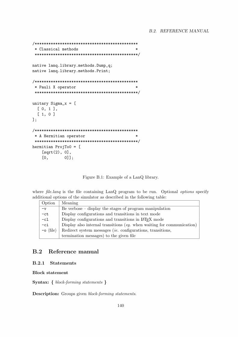
B.2. REFERENCE MANUAL

/********************************************** Classical methods **********************************************/

native lanq.library.methods.Dump_q;native lanq.library.methods.Print;

/********************************************** Pauli X operator **********************************************/

unitary Sigma_x = [[ 0, 1 ],[ 1, 0 ]

];

/********************************************** A Hermitian operator **********************************************/hermitian ProjTo0 = [

[sqrt(2), 0],[0, 0]];

Figure B.1: Example of a LanQ library.

where file.lanq is the file containing LanQ program to be run. Optional options specifyadditional options of the simulator as described in the following table:

Option Meaning-v Be verbose – display the stages of program manipulation-ct Display configurations and transitions in text mode-cl Display configurations and transitions in LATEX mode-ci Display also internal transitions (eg. when waiting for communication)-o 〈file〉 Redirect system messages (ie. configurations, transitions,

termination messages) to the given file

B.2 Reference manual

B.2.1 Statements

Block statement

Syntax: block-forming statements

Description: Groups given block-forming statements.

140

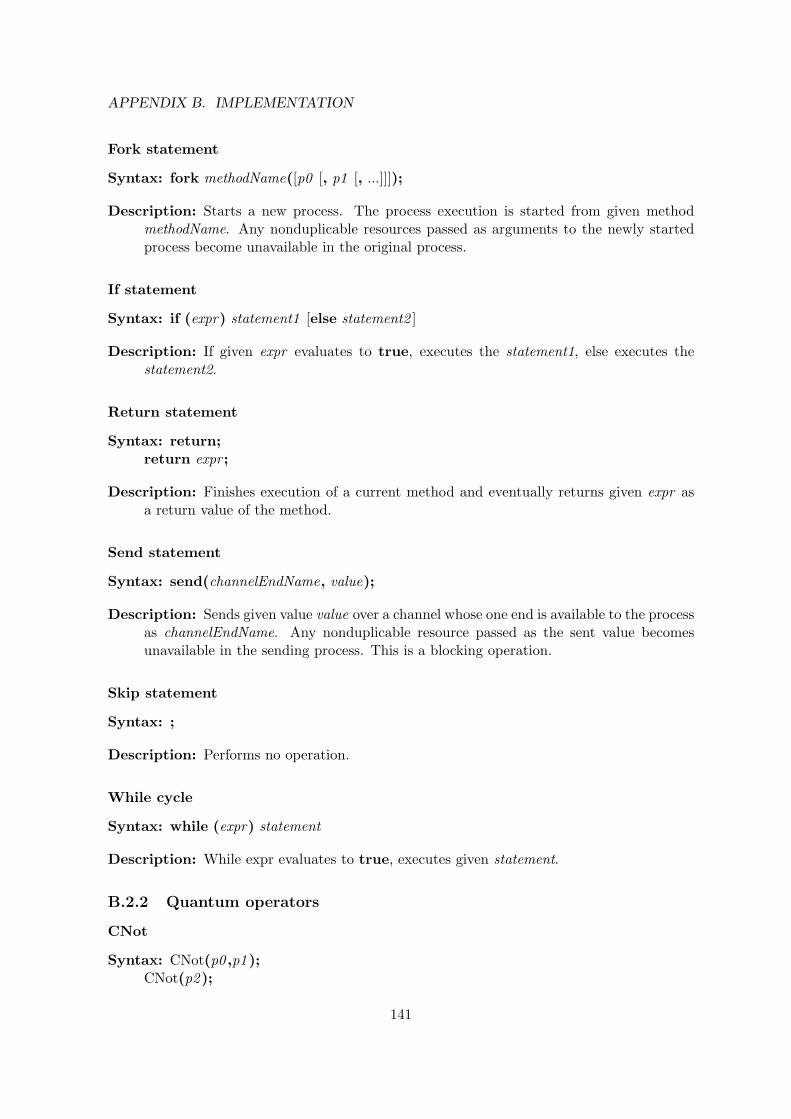
APPENDIX B. IMPLEMENTATION

Fork statement

Syntax: fork methodName([p0 [, p1 [, ...]]]);

Description: Starts a new process. The process execution is started from given methodmethodName. Any nonduplicable resources passed as arguments to the newly startedprocess become unavailable in the original process.

If statement

Syntax: if (expr) statement1 [else statement2 ]

Description: If given expr evaluates to true, executes the statement1, else executes thestatement2.

Return statement

Syntax: return;return expr ;

Description: Finishes execution of a current method and eventually returns given expr asa return value of the method.

Send statement

Syntax: send(channelEndName, value);

Description: Sends given value value over a channel whose one end is available to the processas channelEndName. Any nonduplicable resource passed as the sent value becomesunavailable in the sending process. This is a blocking operation.

Skip statement

Syntax: ;

Description: Performs no operation.

While cycle

Syntax: while (expr) statement

Description: While expr evaluates to true, executes given statement.

B.2.2 Quantum operators

CNot

Syntax: CNot(p0 ,p1 );CNot(p2 );

141

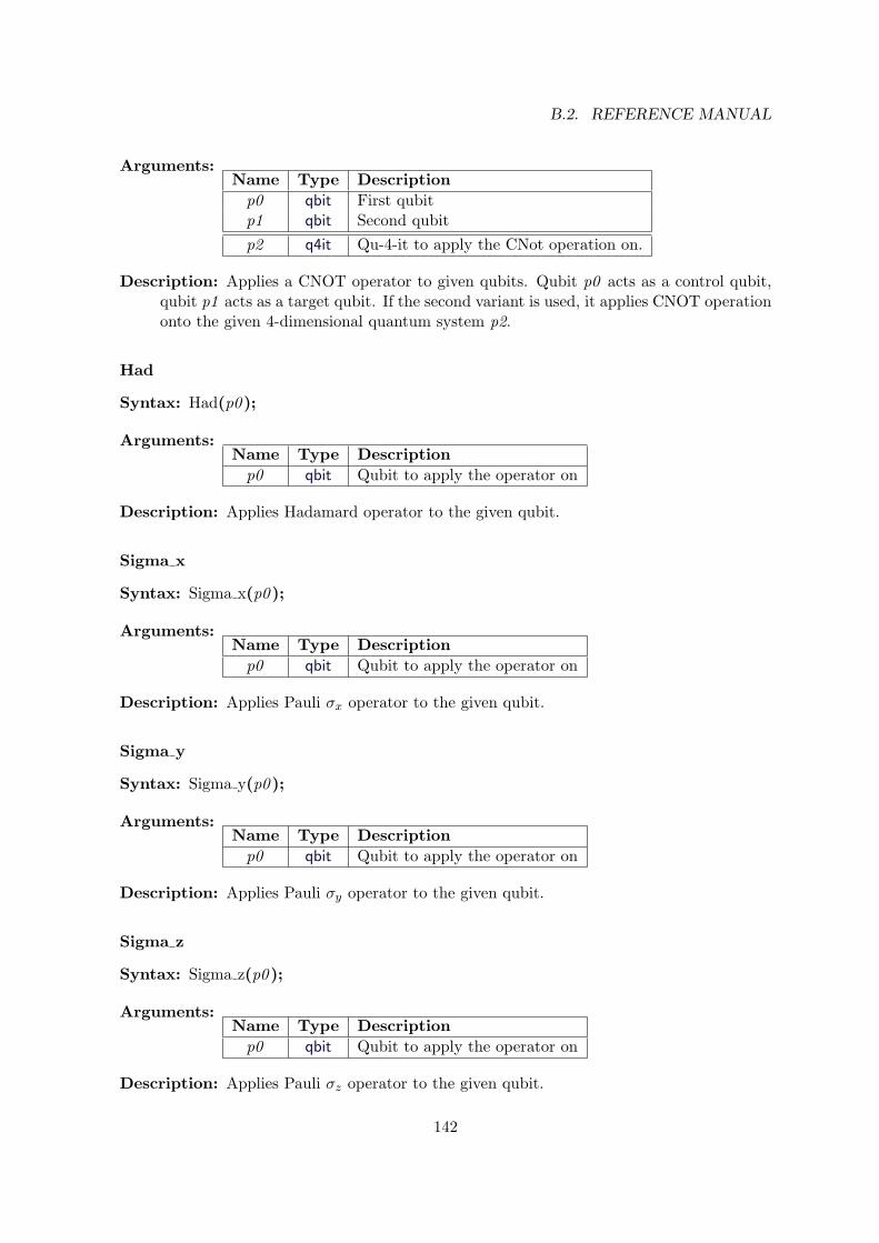
B.2. REFERENCE MANUAL

Arguments:Name Type Description

p0 qbit First qubitp1 qbit Second qubitp2 q4it Qu-4-it to apply the CNot operation on.

Description: Applies a CNOT operator to given qubits. Qubit p0 acts as a control qubit,qubit p1 acts as a target qubit. If the second variant is used, it applies CNOT operationonto the given 4-dimensional quantum system p2.

Had

Syntax: Had(p0 );

Arguments:Name Type Description

p0 qbit Qubit to apply the operator on

Description: Applies Hadamard operator to the given qubit.

Sigma x

Syntax: Sigma x(p0 );

Arguments:Name Type Description

p0 qbit Qubit to apply the operator on

Description: Applies Pauli σx operator to the given qubit.

Sigma y

Syntax: Sigma y(p0 );

Arguments:Name Type Description

p0 qbit Qubit to apply the operator on

Description: Applies Pauli σy operator to the given qubit.

Sigma z

Syntax: Sigma z(p0 );

Arguments:Name Type Description

p0 qbit Qubit to apply the operator on

Description: Applies Pauli σz operator to the given qubit.

142

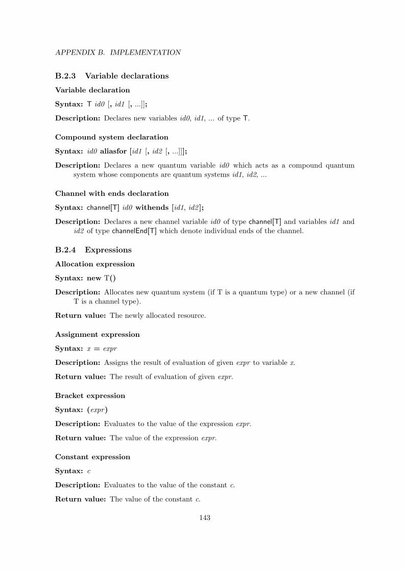
APPENDIX B. IMPLEMENTATION

B.2.3 Variable declarations

Variable declaration

Syntax: T id0 [, id1 [, ...]];

Description: Declares new variables id0, id1, ... of type T.

Compound system declaration

Syntax: id0 aliasfor [id1 [, id2 [, ...]]];

Description: Declares a new quantum variable id0 which acts as a compound quantumsystem whose components are quantum systems id1, id2, ...

Channel with ends declaration

Syntax: channel[T] id0 withends [id1, id2 ];

Description: Declares a new channel variable id0 of type channel[T] and variables id1 andid2 of type channelEnd[T] which denote individual ends of the channel.

B.2.4 Expressions

Allocation expression

Syntax: new T()

Description: Allocates new quantum system (if T is a quantum type) or a new channel (ifT is a channel type).

Return value: The newly allocated resource.

Assignment expression

Syntax: x = expr

Description: Assigns the result of evaluation of given expr to variable x.

Return value: The result of evaluation of given expr.

Bracket expression

Syntax: (expr)

Description: Evaluates to the value of the expression expr.

Return value: The value of the expression expr.

Constant expression

Syntax: c

Description: Evaluates to the value of the constant c.

Return value: The value of the constant c.

143

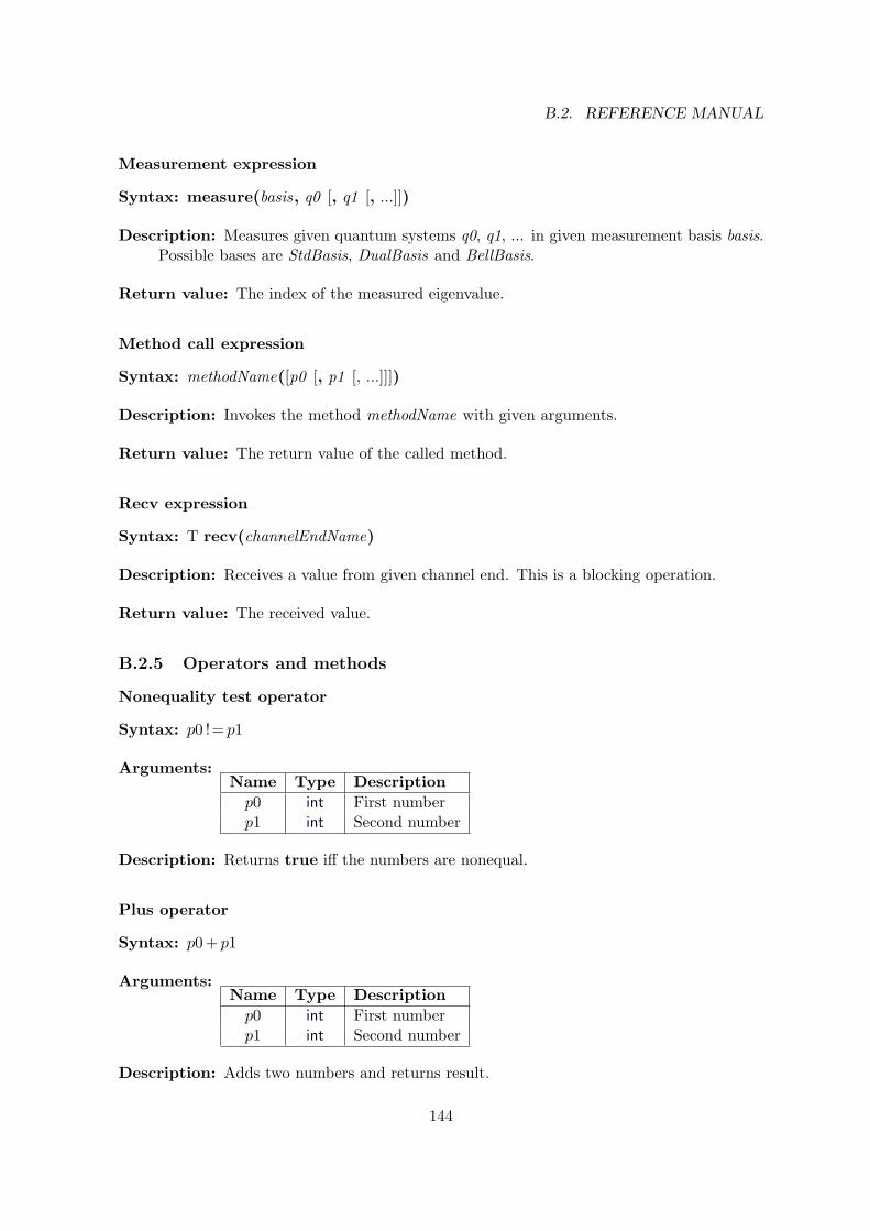
B.2. REFERENCE MANUAL

Measurement expression

Syntax: measure(basis, q0 [, q1 [, ...]])

Description: Measures given quantum systems q0, q1, ... in given measurement basis basis.Possible bases are StdBasis, DualBasis and BellBasis.

Return value: The index of the measured eigenvalue.

Method call expression

Syntax: methodName([p0 [, p1 [, ...]]])

Description: Invokes the method methodName with given arguments.

Return value: The return value of the called method.

Recv expression

Syntax: T recv(channelEndName)

Description: Receives a value from given channel end. This is a blocking operation.

Return value: The received value.

B.2.5 Operators and methods

Nonequality test operator

Syntax: p0 != p1

Arguments:Name Type Descriptionp0 int First numberp1 int Second number

Description: Returns true iff the numbers are nonequal.

Plus operator

Syntax: p0 + p1

Arguments:Name Type Descriptionp0 int First numberp1 int Second number

Description: Adds two numbers and returns result.

144

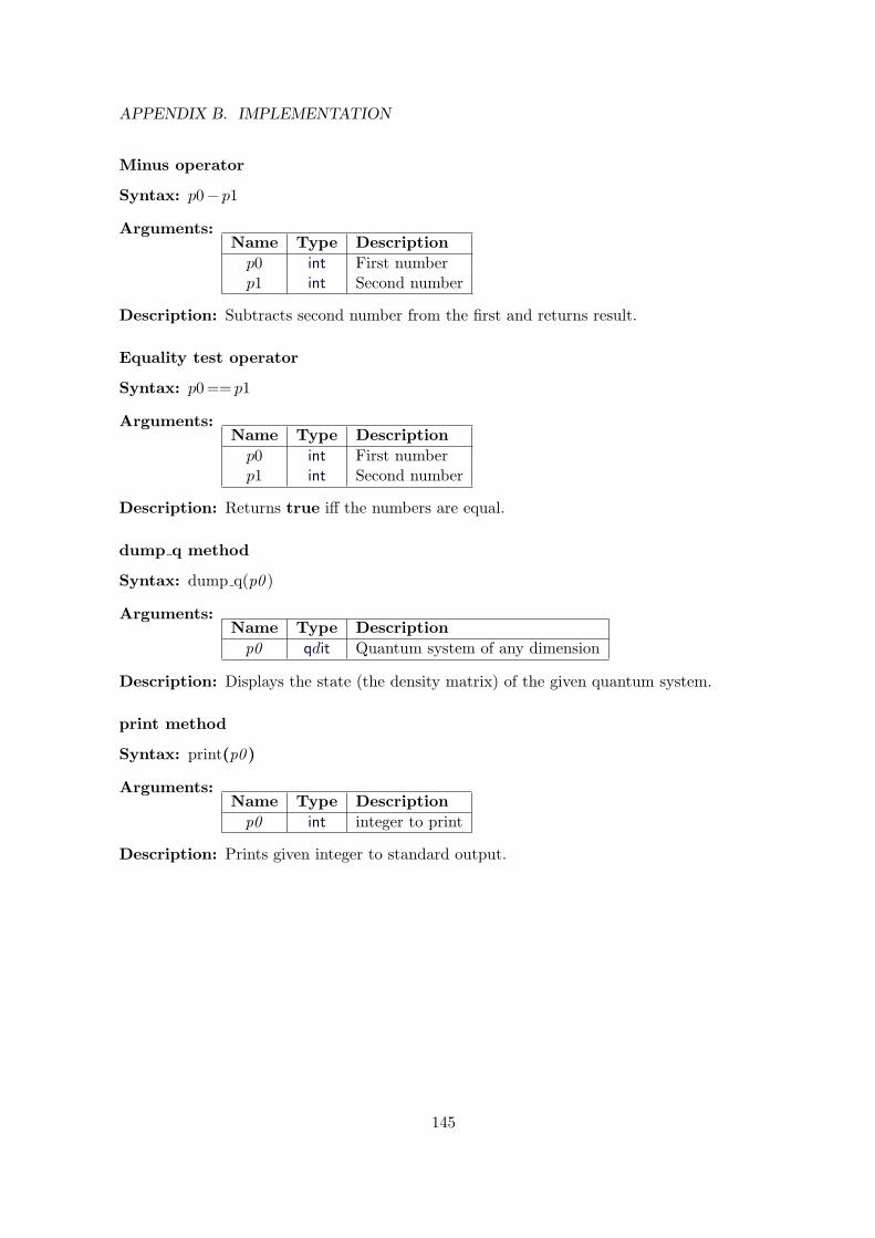
APPENDIX B. IMPLEMENTATION

Minus operator

Syntax: p0− p1

Arguments:Name Type Descriptionp0 int First numberp1 int Second number

Description: Subtracts second number from the first and returns result.

Equality test operator

Syntax: p0 == p1

Arguments:Name Type Descriptionp0 int First numberp1 int Second number

Description: Returns true iff the numbers are equal.

dump q method

Syntax: dump q(p0 )

Arguments:Name Type Description

p0 qdit Quantum system of any dimension

Description: Displays the state (the density matrix) of the given quantum system.

print method

Syntax: print(p0 )

Arguments:Name Type Description

p0 int integer to print

Description: Prints given integer to standard output.

145