quantum mesoscopic scattering: disordered systems and
TRANSCRIPT
HAL Id: jpa-00247057https://hal.archives-ouvertes.fr/jpa-00247057
Submitted on 1 Jan 1995
HAL is a multi-disciplinary open accessarchive for the deposit and dissemination of sci-entific research documents, whether they are pub-lished or not. The documents may come fromteaching and research institutions in France orabroad, or from public or private research centers.
L’archive ouverte pluridisciplinaire HAL, estdestinée au dépôt et à la diffusion de documentsscientifiques de niveau recherche, publiés ou non,émanant des établissements d’enseignement et derecherche français ou étrangers, des laboratoirespublics ou privés.
Quantum Mesoscopic Scattering: Disordered Systemsand Dyson Circular Ensembles
Rodolfo Jalabert, Jean-Louis Pichard
To cite this version:Rodolfo Jalabert, Jean-Louis Pichard. Quantum Mesoscopic Scattering: Disordered Systems andDyson Circular Ensembles. Journal de Physique I, EDP Sciences, 1995, 5 (3), pp.287-324.�10.1051/jp1:1995128�. �jpa-00247057�

J. Phys. I France 5 (1995) 287-324 MARcH1995, PAGE 287
Classification
PA ysics Abstracts
05.608 72.10B 72.15R 72.20M
Quantum Mesoscopic Scattering: Disordered Systems and DysonCircular Ensembles
Rodolfo A. Jalabert (~,2) and Jean-Louis Pichard (~)
(~) CEA, Service de Physique de l'Etat Condensé, Centre d'Études de Saclay, 91191 Gif-sur-
Yvette Cedex, France
(~) Division de Physique Théorique(*), Institut de Physique Nucléaire, 91406 Orsay Cedex,France
(Received 9 September1994, accepted December1994)
Abstract. We consider elastic reflection and transmission of electrons bya
disordered sys-
tem characterized by a 2N x 2N scattering matrix S. Expressmg S in terms of the N ra-
dial parameters and of the four NM N unitary matrices used for the standard transfer matrix
parametrization, we calculate their probability distributions for the circular orthogonal (COE)and unitary (CUE) Dyson ensembles. In this parametrization, we explicitly compare the COE-
CUE distributions with those suitable for quasi-id conductors and insulators. Then, returningto the usual eigenvalue-eigenvector parametrization of S,
we study the distributions of the scat-
tering phase shifts. For a quasi-id metallic system, lriicroscopic simulations show that the phaseshift density and correlation functions
areclose to those of the circular ensembles. When quasi-
id longitudinal localization breaks S into two uncorrelated reflection matrices, the phase shift
form factor b(k) exhibits a crossover from a behavior characteristic of two uncoupled COE-CUE
(small k) to asingle COE-CUE behavior (large k). Outside quasi-one dimension, we find that
the phase shift density is no longer uniform and S remains nonzero alter disorder averagmg. We
use perturbation theory to calculate the deviations to the isotropic Dyson distributions. When
the electron dynamics is no longer zero dimensional in the transverse directions, small-kcorrec-
tions to the COE-CUE behavior of b(k) appear, which are relriiniscent of the dimensionality-dependent non-universal regime of energy level statistics. Using
aknown relation between the
scattenng phase shifts and the system energy levels, we analyse those corrections to the universal
random matrix behavior of S which result from d-dimensional diffusionon
short time scales.
l. Introduction
The discovery of universal conductance fluctuations [1-3] (UCF characterizing trie sensitivity
of trie conductance of small metallic samples to a change of trie Fermi energy, magnetic field
or impurity configuration) bas geuerated a sustained interest in quantum mesoscopic physics
(*) Unité de Recherche des Universités Paris XI et Paris VI associée auCNRS.
© Les Editions de Physique 1995
288 JOURNAL DE PHYSIQUE I N°3
since the mid eighties. Mesoscopic systems have a size of the order of the electron phase-coherence length L~, 1-e- a scale intermediate between single atoms (microscopic) and bulk
solids (macroscopic). First, it is in terms of quantum interference between diiferent multiplescatteriug paths that UCF has been understood [2, 3]. The umversality of the phenomenon(reproducible fluctuations of order e~ /h, independently of the mean conductance) quickly lead
physicists [4, Si to understand UCF as a signature of a more general universality resulting from
the eigenvalue correlations of random matrices.
The standard random matrix ensembles were introduced in the context of Nuclear Physics[6-9] and later found to also descnbe the statistical properties of quantum systems whose
classical analogs are chactic [10,11]. Contrary to a microscopic approach where the systemHamiltoniau H, scattering matrix S or transfer matrix M result from a more or less arbitrarydistribution of the substrate potential, random matrix theory (RMT)
assumes for H, S or M
statistical ensembles resulting from an hypothesis of maximum randomness, given the systemsymmetries (time-reversal symmetry, spin rotation symmetry, current conservation) plus a few
additionnai constraints.
A direct relationship between conductance fluctuations and RMT comes from the Thouless
expression of the conductance
~2G
=N(E~)
,
(1.1)
given by the number of one-electron (~) levels N(E~) which lie within an energy bond of width
E~=
Dh/L~ centered around the Fermi energy Ef. The Thouless energy E~ is the inverse
characteristic time for an electron to diffuse through the sample (of size L). The electron
diffusion coefficient is D=
ufl/d, where vf is the Fermi velocity, the elastic mean free path,and d the spatial dimension of the sample. Fluctuations in the number of levels within E~ are
therefore related to conductance fluctuations. The analysis of fluctuations in the spectrum of
non-interacting electrons in metallic partides was initiated by Gorkov aud Eliashberg [12]. The
relevance of RMT was proved by Efetov [13] and complemented by Altshuler and Shklovskii [4]who noticed non-RMT behavior for energy separations larger thon E~. Using a diagramaticperturbation theory for the density-density correlation function in the weak disorder limit
kl » 1 (k is the Fermi wave vector), they showed that the correlation between energy levels is
correctly described by the universal RMT laws for energy scales smaller thon E~, but is weaker
(and dimensionality dependent) beyond Ec(~).Pionieered by Imry [Si, an alternative approach relating UCF and random matrix theories is
based on the Landauer formula, which gives the conductance in terms of the total transmission
coefficient of the sample (at the Fermi energy), considered as a single, complex elastic scatterer.
For a twc-probe measurement where the disordered sample is attached between two perfectreservoirs with an infinitesimal diiference m their electrochemical potentials, the conductance
(measured in units of e~/h) is
g =Tr[ttt] (1.2)
The transmission matrix t con be expressed in terms of the transfer matrix M, for which a
standard random matrix theory ("global approach") has been developed [14,15]. A set of N
(~)Throughout this work we will treat spinless electrons and thereforewe
will not write spin-degeneracy jactons.
(~) This limit oi the universal RMT lawsis
specifically denved ignonng electron-electron interaction.
N°3 SCATTERING IN DISORDERED SYSTEMS 289
real positive parameters describing the radial part of the 2Nx 2N transfer matrix M (precisedefinitions are given m the next section) are trie relevant "eigenvalues" in this approach, and
their probability distribution is
P(lÀal)= exP (-fl7i(lÀal))
,
(13)
N N
7i(lÀal)"
£ '°g lÀa Àbl + £ V(Àa) (1.4)a<b a=i
This is trie usual RMT Coulomb gas analogy with logarithmic pairwise interaction, a systemdependent confining potential V(À), and an inverse temperature fl
=1, 2,4 depending on trie
system symmetries. This distribution corresponds to trie most random statistical ensemble for
M given trie average density p(À) of radial parameters, which controls trie average conductance
(g). In this maximum entropy ensemble, V(À) and p(À) are related by an integral relation m
trie large N-limit [16]:
C is a constant, and to leading order in N this mean-field equation expresses trie equilibriumof a charge at resulting from its interaction with the remaining charges and the confiningpotential.
In this work we examine the statistical properties of another matrix related to quantumtransport in disordered systems: the scattering matrix S.
First, the relation between M and S is straightforward, since M con be expressed in terms
of the reflection and transmission submatrices which define S. This allows us to show that
the À-statistics characterizing the Dyson ensembles coincides with a "global approach" for
M, given a particular confining potential V(À). Using this equivalence, the detailed proofof it being given in this work, the quantum transport properties associated with the circular
ensembles bave been obtained [17], including trie weak-localization eifects and the quantumfluctuations of various linear statistics of trie À-parameters (conductance, shot-noise power,
conductance of a normal-superconducting microbridge, etc). This equivalence bas also been
derived by Baranger and Mello [18], and bas been confirmed in their numerical simulations of
chaotic billiards.
Second, smce S is unitary, its 2N eigenvalues (exp (19m)) are just given by the 2N phaseshifts (9m). In the Dyson circular ensembles, where all matrices S with a given symmetry
are equally probable, the phase shift statistics follow trie same universal level correlations thon
in the Gaussian ensembles of corresponding symmetry. The applicability of Dyson circular
ensembles for chactic scattering bas been established by the pioneering work of Blümel and
Smilansky [19], as for as trie twc-level form factor for trie phase shifts is concerned. Further
evidence comes from numerical studies of 2 x 2 matrices describing trie scatteriug through
chactic cavities [20].However, a ballistic chaotic cavity, with a conductance of order N/2 and where the electronic
motion is essentially zero-dimensioual after a(short) time of flight, diifers from a disordered
conductor or insulator. The introduction of bulk disorder in the dot reduces the conductance to
smaller values of order Ni IL (L »,
metallic regime) and enhances the time interval iii which
the electron motion depends on system dimensionality. Trie diifusive motion of trie carriers
after a(short) characteristic time Te limits (rather thon improves) the validity of the standard
RMT distributions. The subject of this study consists precisely m understanding this apparent
290 JOURNAL DE PHYSIQUE I N°3
paradox: the fact that the introduction in a cavity of bulk disorder drives the statistics of S
away from the circulai ensembles. For this p1÷rpose, we extensively study disordered systems
where non-interacting electrons are elastically scatterered by microscopic imp1÷rities contained
m a rectangular dot of various aspect ratios. We derive 1÷seful relations between diiferent
parametrizations of H, M and S, involving the energy levels (E,), the radial parameters (Àa)and the phase shifts (9m).
The paper is organized as follows. After presenting the basic definitions of oui mortel and the
relationship between S and M, we derive (Sect. 3) trie metric of S in trie polar decomposition,and therefore trie probability distribution of trie radial parameters assuming a Dysou distri-
bution for the scattering matrix iii trie time-symmetric case (the case without time-reversal
symmetry is worked in Appendix D). In Section 4 we use this parametrization to discuss the
diiferences and similarities between the circular ensemble distributions and those suitable for
quasi-one dimensional disordered systems. In Section 5 we start the statistical analysis of the
phase shifts of S for long conductors with weak disorder. In Section 6 we study the scatteringphase shifts in quasi-là insulators and show that their correlations are well described by those
of two uncoupled circular ensembles. In Section 7 we calculate by diagrammatic perturba-tion theory trie mean values of trie S-matrix, which are needed to understand trie phase shift
anisotropy fo1÷nd outside trie weak disorder, quasi-là limit. In Section 8 we present numerical
results for geometries other than quasi-one dimensional strips (1.e. squares and thin slabs) and
show that, after trie spectrum is unfolded, there is a rougir agreement with trie circular ensem-
bles, though noticeable discrepancies are visible in trie number variance. These deviations are
analyzed in Section 9, using the known deviations of metallic spectra from the R-M.T. behavior
and exploiting a relationship betweeu scatteriug phase shifts and the energy levels (AppendixB). Appendix A gives a summary of the methods and results of the numerical simulations,and in Appendix C, we use a semidassical approach to complement our understauding of the
res1÷lts, induding the meaning of the Wigner time.
2. Scattering, Transfer, Transport and À-Parameters
Using only the system symmetries (current conservation, time reversai symmetry, spin rotation
symmetry) one can show that both S and M can be expressed in terms of the N radial
parameters (Àa) of M and 4 (2 in the presence >of time reversai symmetry) N x N auxiliaryunitary matrices. In this parametrization, we shall show the similarities and the diiferences
between the distributions implied by the circular ensembles and those describing in the weak
scattering limit long quasi-là disordered conductors and insulators. To make concrete our
explorations, we introduce in what follows the essential elements of the particular microscopicmortel on which we test the validity of Dyson circular ensembles.
We consider an mfinite strip composed of two semi-infinite perfectly conductiug leads of
width L~ connected by a disordered part of same width and of longitudinal length L~ (Fig. l).Assuming non-mteracting electrons and hard-wall boundary conditions for trie transverse partof the wavefunction, the scattering states m the leads at the Fermi energy Ef
=
h~k2 /2m sat-
isfy the condition k2=
(n7r/L~)2 + k(, where k is the Fermi wavevector, n7r/L~ the quantizedtransverse wavevector and kn the longitudinal momentum. The various transverse momenta
labeled by the index n(n
=1,...,N) which satisfy this relationship with k( > 0 defiue the
N propagating charnels of the leads. Since each channel can carry two waves travelling m
opposite directions, asymptotically for from trie disordered region trie wave function can be
specified by a 2N-component vector on trie two stries of the disordered part. Iii each lead trie
N°3 SCATTERING IN DISORDERED SYSTEMS 291
A C
B y ~
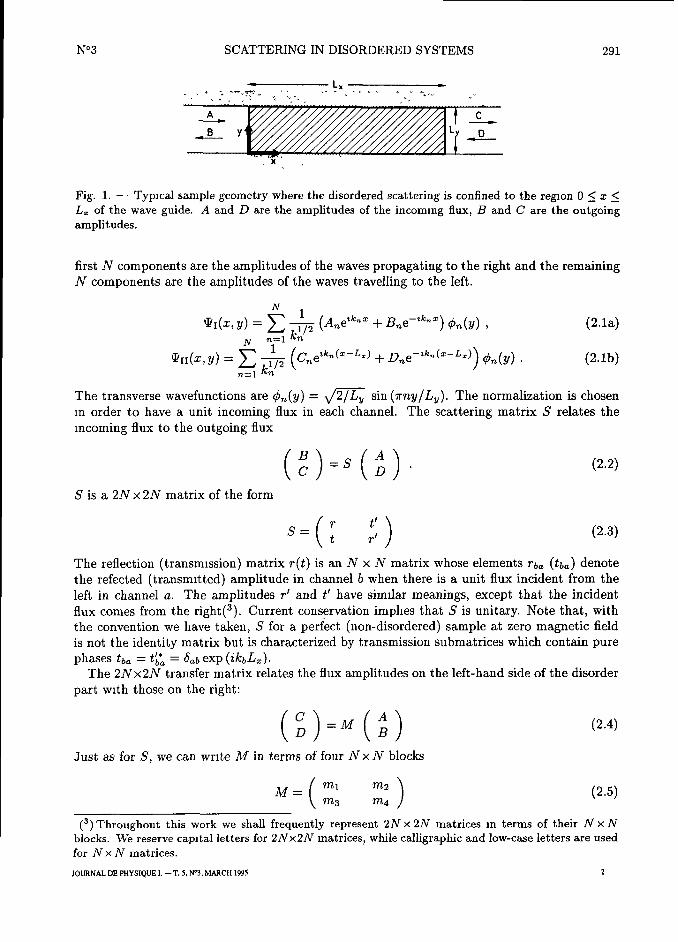
Fig. l. Typical sample geometry where the disordered scattering is confined to trie region 0 <z <
L~ of thewave
guide. A and D arethe amplitudes of the incomiug flux, B and C
arethe outgoing
amplitudes.
first N components are trie amplitudes of trie waves propagating to trie right and trie remainiugN components are trie amplitudes of trie waves travelling to trie left.
i~I(x,Yj=
( jiA»e~kn~ + B»e-~kn~) <»(y)
,
(~.ia)
4ÎII(X, il)=
£ £(Cne'~"~~~~~l + Dne~'~"~~~L~)) ~b~(y) j2,ib~
~=~kn
The transverse wavefunctions are #n(g)=
fi sin(7rng/L~). Trie normalization is chosen
m order to bave a unit incoming flux in each channel. Trie scattering matrix S relates trie
mcomiug flux to trie outgoing flux
1$ =S (2.2)
S is a 2N x 2N matrix of trie form
S=Î
(2.3)~
The reflection (transmission) matrix r(t) is an N x N matrix whose elements rôa (tôa) denote
trie refected (transmitted) amplitude in channel b when there is a unit flux incident from trie
left in channel a. Trie amplitudes r' and t' bave similar meanings, except that trie incident
flux comes from trie right(~). Current conservation imphes that S is unitary. Note that, with
trie convention we bave taken, S for a perfect (non-disordered) sample at zero magnetic field
is not trie identity matrix but is characterized by transmission submatrices which contain pure
phases tôa"
t[[=
ôaô exp (ikôL~).Trie 2Nx2N transfer matrix relates trie flux amplitudes on trie left-baud side of trie disorder
part with those on trie right:
l~=M
~ (2.4)D B
Just as for S, we can wnte M in terms of four NXN blocks
M=
l~~ ~~ (2.5)m3 m4
(~)Throughout this work weshall frequently represent 2N x 2N matrices in terms of their NM N
blocks. We reservecapital letters for 2Nx2N matrices, while calligraphic and low-case letters are
used
for NM N matrices.
JOURNAL DE PHYSIQUE1. T. 5, Nô, MARCH1995 2
292 JOURNAL DE PHYSIQUE I N°3
The reflection and transmission matrices of S con be expressed in terms of trie block matrices
m, of M. Introducing trie polar representatiou [21, 22] of M, we bave:
r =
-m[~m3"
-u~~)Ru~~),
(2.6a)
t=
(m()~~=
ul~)Tu~~),
(2.6b)
r'=
m2mj~=
u~~)Ru~~),
(2.6c)
t'=
ml=
u(~)Tu(~),
(2.6d)
where u(~) (l=
1,...,4) are arbitrary N x N unitary matrices. R and T are real diagonalNx N matrices whose non-zero elements (labeled by only one index) are trie square roots of
trie reflection and transmission eigenvalues, which can be expressed as a function of trie real
positive diagonal elements Àa (a=
1,.,
N) of trie NXN diagonal matrix characterizing trie
radial part of M:
à 1/2
~~ ~l +~Àa~~'~~~
i1/2
~1
+ Àa~~'~~~
Iii this À-parametrization, M and S can then be written as
M=
[~~ ~i~~ (Iji)i~/~~(~[(i/~ [~ ~ij~
,~~.~~
~(3) o _~ ~- ~(l) o~
~ ~(4) ~- ~ ~ ~(2) (~.~)
Since ttt=
uiT~u), trie dimensionless conductance con be expressed as
~ i~1 Àa
~~'~~~
The conductance is therefore a hnear statistics of trie radial parameters (Àa) of M. Note that
s1÷ch a simple relationship does not exist between g and trie scattering pliase-shifts (9a), since
trie relation between trie eigenval1÷es of S and those of ttt depends on trie eigenvectors of S
and on trie u-matrices.
In trie absence of a maguetic field there is time-reversal symmetry, trie S-matrix is symmetric(S
=
S~) and trie polar decomposition bas only two arbitrary 1÷nitary matrices since
u(3)~
~jl)T j~ 11 ~~
u14j~
~j2)T j~ ~~~~
In this case trie number of independeut parameters is to 2N2 + N. We bave N2 parametersfor each of trie two N x N unitary matrices and N for trie diagonal matrix À. Without time-
reversal symmetry (unitarycase with spin degeneracy) trie number of indepeudent parameters
of S land M) is 4N2 (trie N extra parameters of trie polar decompositions (2.9) and (2.8) are
due to trie fact that theyare not unique ils] ). In trie symplectic case occurring when there is
a strong spin-orbit scattering m trie disordered part and no applied magnetic field, trie spindegeneracy is removed and each matrix element becomes a 2 x 2 quaternion matrix, which
doubles trie size of M and S, but ul~) and u(~)are also given [22] in terms of u(~) aud u(~) and
trie bave a twofold degeneracy (Kramers degeneracy).
N°3 SCATTERING IN DISORDERED SYSTEMS 293
3. Invariant Measure of S in the Polar Decomposition
In this section we calculate trie invariant measure p(dS) of S in terms of trie radial parameters(Àa) and trie matrices u~~) We present here trie time-symmetric case (fl
=1), while trie
unitary case (fl=
2) relevant when a magnetic field is applied is considered in Appendix D.
Our calc1÷lations bave recently been extended by Frahm [23] for trie symplectic case (fl=
4).In trie orthogonal case S is 1÷nitary symmetric and can be decomposed as:
s=wTzw=uTru=YTY. (3.i)
The first equality simply means trie diagonalizatiou of S and introduces trie 2N phase shifts
of S through trie diagonal elements exp(19m) of Z and a 2N x 2N orthogonal matrix W
containing trie eigenvectors of S. Trie second equality results of trie polar representation of S
where trie real matrix r and trie block-diagonal unitary matrix U are giveu by equation (2.9)with conditions (2.Il). Trie last decomposition holds for any unitary symmetric matrix and
introduces a 2N x 2N unitary matrix Y which is not unique, but specified up to an orthogonaltransformation. Following Dyson [7], trie measure of
aneighbourhood dS of S is given m
terms of trie infinitesimal variations dÙ~j of trie matrix elements of a real symmetric matrix
dû defined by:
dS=
Y~ (idù) Y,
(3.2)
2N
p(dS)=
fl dM~j (3.3)
>ij
This definition is independent of trie particular choice of trie unitary matrix Y and we use this
freedom of choice to take a convenient Y for expressingdû in trie À-parametrization. To this
end, we note that r is real symmetric and unitary, with eigenvalues +1 and diagonalizable by
an orthogonal transformation O:
r=
oT D o, (3.4)
D=
~°
-
Il(3.5)
The NXN blocks of O are diagonal matrices given by
~~ v5~'
~~ Vi~ ~~~~
Writing trie diagonal matrix D asF2, with
F=
.j,
(3.7)~
one can write 5 asY~Y, with
~ ~ ~ ~ Î~ÎÎ~~I -iÎÎ~~~ ~~'~~

294 JOURNAL DE PHYSIQUE I N°3
Since Y is unitary, its infinitesimal variations can be expressed as
dY=
ôY Y, (3.9)
where trie matrix ôY is antihermitic. Analogously, for trie block components of U we can write
du(~l=
ôu(~) u(~),
ôu(~)=
da(~) + i dsl~),
1=1, 2. (3.10)
da(~) (ds(~)) are real antisymmetric (symmetric) Nx N matrices. Trie Haar measure p(du(~l)for trie unitary matrices u(~l satisfies p(du(~))
=fl~ dsl) fl~~~daf/dsf/. Therefore trie in-
finitesimal variations of Y and S are given by
~ i (dQ P d~' ~~+ôY
" j (dQ P dP Q) ~
~i
Q~ÎÎÎ~~IÎ-Î'~ÎÎÎ~~)~)~ ~Î~ôÎÎÎ~~~~ÎÎÎÎÎÎ~Î'~~
'
~~'~~~
dS=
Y~(ôY ôY*)Y=
Y~(idù)Y (3.12)
This gives us trie real symmetric matrix dû in terms of the radial parameters (Àa ), the unitarymatrices u(~) and their infinitesimal variations (dÀa) and ôu(~). We just need to calculate a
Jacobean which can be decomposed as the product of three determinants,
(3.13a)p~ N
1~ ~~
,
§ dÙa,a+N §2/Ç(1 + ~a~
ama>à+Ndmôa+N =1 2
Il Ilda~~~da~~~ (3.13b)
j~~~'~~~~~~'~~~ ij ~ Î~~~~~~~ j~ ~
~Î~
Î~~~~~~~
'
~ ~ ~~
(3.13c)which eventually gives for the invariant measure of the symmetric unitary matrix S
~~~~~ §(l +
a)3/~ §l
/Àa 1
/Àô
~~~~~ ~~~"~~~~ ~~'~~~
in terms of the measure p(dÀ)=
fl$~~ dÀa of the matrix and of the Haar measures p(du(~))of the matrices u(~)
4. Dyson Circular Ensembles and Quasi-lD Disordered Systems
For the Dyson circular ensembles the number of S-matrices in a volume element dS of measure
p(dS) around a given S is just proportional to p(dS):
P(dS)=
)p(dS)
,
(4.1)
N°3 SCATTERING IN DISORDERED SYSTEMS 295
V is a normalization constant. Using the À-parametrization,one obtains that the matrices
u(~)are independent of each other (except by symmetry relations) and distributed according to
the invariant Haar measure on the unitary group, while the N parameters Àa are statisticallymdependent of the u-matrices and have a joint probability distribution which can be expressed
mthe usual Coulomb gas analogy as a Gibbs function
P(lÀal)= exP (-fl7i(lÀal)) 14.2)
The symmetry parameter fl plays the role of an inverse temperature and the effective Hamil-
tonian 7i is characterized by a logarithmic pairwise interaction and a one-body potential:
N N
7i(lÀal)"
£ f(Àa> Àb) + £ V(Àa) (4.3)
a<b a=i
/(à~, à~)=
-iogjà~ à~j,
j4.4)
VIA)- IN + ~ù~l '°~ ii + À) 14.5)
This Coulomb gas analogy characterizes the orthogonal, unitary and symplectic ensembles
which ailler not only by the value of the "temperature" fl~~, but also by the presence ofa
small fl-dependent correction to the leadiug behavior of VIA) in a large N-expansion. It
is remarkable that the pairwise interaction for the À-parameter is the same as in the globalmaximum entropy approach to the transfer matrix ils], while V(À) diifers
m two important
aspects: it is essentially proportional to log instead of log~ [24] for large values of À, and the
prefactor is just the number of modes N instead of the classical conductance Nl/L~. These
diiferences are not surprising since forward and backward scatterings are essentially put on the
same footing in the circular ensembles, leading to a total transmission intensity of the order of
the total reflection intensity, T m R mN/2 (up to weak-localization corrections) [17,18]. For
a disordered conductor or insulator, the refection R is much larger than the transmission T.
Clearly, bulk diffusion characterized by an elastic mean-free-path cannnot be described by the
circular ensembles, which are appropriate for systems where an injected carrier is subjected to
a chactic dynamics before finding (with equal chance) one of the two injection leads. However,
as shown by Beenakker [25], in the large N-limit, the density-density correlation function
(and therefore the variance of any linear statistics hke the conductance) depends only on the
pairwise interaction, and net on the particular form for V(À). Consequently, bath the circular
ensembles and the global maximum entropy approach to the transfer matrix yield identical
UCF [26] values 2/(16fl), slightly diiferent from the perturbative microscopic result [2,3] for
quasi-là disordered conductors 2/(lsfl).In the polar representation of S, one can precisely see the diiference between the circular
ensembles and those appropriate for quasi-one dimensional disordered systems. For this, we
just need to recall what we know from another statistical approach introduced for arbitrary N
by Dorokhov [27] from microscopic considerations and by Mello et ai. [21,28] froma maximum
entropy assumption for the infinitesimal transfer matrix of the building block of a quasi-là
serres. These works are based on an isotropy hypothesis: it is assumed that the u-matrices
are distributed with the Haar measure on the unitary group and statistically independent from
the radial part of M (see Eq. (2.8)). This limits their conclusions to quasi-one dimension and
yields aFokker-Planck equation for P((Àa )) which implies the same UCF and weak-localization
corrections for quasi-là conductors as those given by diagrammatic calculations. The evolution
296 JOURNAL DE PHYSIQUE I N°3
of P((Àa)) witl the length L~ of the disordered part is given by a heat equation where the
Laplacian becomes trie radial part of the Laplace-Beltrami operator on a space of uegative
curvature. Using Sutherland's transformation, Beenakker and Rejaei [29] have mapped this
diffusion equation on to a Schrôdinger equation (with imagmary time) of a quantum set of
point-like partiales free to move on a half fine (the positive part of the real axis) within a certain
potential. For arbitrary values of fl, these partiales have a pairwise interaction, attractive for
fl=
1 and repulsive for fl=
4, making it diilicult to find the solution. Fortunately, this
interaction vanishes for fl=
2, and the solution of the diffusion eq1÷ation is red1÷ced to an
exactly solvable quantum N-body froc fermion problem. This gives for the unitary case a
pairwise interaction
f(Àa Àô)"
In )Àa Àô) In ~arcsinh~(/~) arcsmh~ (fi)
,
(4.6)2 2
which reduces to the usual logarithmic interaction assumed by the global approach for )Àa
Àô) < 1, but which is halved if )Àa Àô) » 1 in the quasi-là dilfusive or localized limit. This
discrepancy is responsible for trie slightly diiferent UCF values characterizing ballistic quantumdots with chaotic dynamics and quasi-là disordered conductors.
In the localized regime, the global and local approaches give identical symmetry dependenceof the localization lengths, though the (log) conductance fluctuations ailler by a factor 2 in
the quasi-là localized limit [30]. The latter point again is consistent with the halving of the
pairwise interaction f(Àa Àô) for large eigenvalue separations given by the local approach. For
metals aria insulators far from a quasi-one dimensional shape, a more dramatic shrinkage of the
validity of the universal RMT-correlations has been observed [24]. This means that transverse
diffusion (oreven more transverse localization [31]) yields a more significant reduction of the
RMT pairwise interaction than that obtained in quasi-one dimension by Beenakker and Rejaei.To address this problem, we return to the study of the more familiar scattering phase shifts of
S.
5. Scattering Phase Shifts in Quasi-lD Metals and a Single Circular Ensemble
As discussed in the previous section, when applied to quasi-là conductors, trie circular ensem-
bles give trie right statistics for trie u-matrices, and locally trie correct interaction f(Àa, Àô), but
certainly not trie appropriate confining potential V(À). Using now trie eigenvalue-eigenvectorparametrization of S, we study trie phase shift distribution in trie case of weak disorder and
quasi-là samples. We first introduce trie basic notation, then write trie expected universal
correlation for Dyson ensembles, which we compare to our numerical results.
Since the S-matrix is unitary, its 2N eigenvalues are given by 2N phase shifts 9m. FollowingBlümel and Smilansky [19] we write the phase shift deusity as
Mco
p(9)=
~ (ô(9 9m)j= ~
~exp (-in9)jTr S"1
,
(5.ljm=1
~n=-co
where the angular brackets mdicate average over the ensemble of disordered sarnples and M=
2N is the dimension of S. The two-point corielation function R2 is defined by
M
R2(61,62)=
~j (à(61 6m)à(92 6m,)) (5.2)
m#m'
N°3 SCATTERING IN DISORDERED SYSTEMS 297
When the phase-shift distribution is uniform (p(9)=
M/27r) the two-point correlation function
depends only on the diiferenceJ~ =
92 91,
R2(11)"
) f((()Tr S'~)~) l) exp (inJ~) (5.3)
The twc-level cluster function is defined, for the reduced variable r =J~M/27r, in the limit
where the number of phases M goes to iufinity,as:
Y2(r)=
lim É~~(r),
(5.4)M-ce
~~~~ ~ÎÎ~ l~Î~ ~~~ÎÎ~~
~~'~~
Using expression (5.3) we bave
t'~(r)=
ùIi 2
Ése
Cos (~]~),
(5.6)
»=1
where Fourier components se are giveu by
se=
((jTr snj2) -1 (s.7)
The argument r of trie cluster f1÷nction goes from -co to +co, and trie Fourier transform of
Y2, trie two-level form factor (TLFF), is given by
b(k)=
j~dr Y2(r)exp(27rikr) (5.8)
Comparing trie Fourier transform of Y2 and trie Fourier coefficients of É~~ in trie large M limit,
we can identify
sem
b(n/M),
M » (5.9)
For matrices S belon#ng to Dyson ensembles, trie distribution of phase shifts is given bytrie Co1÷lomb gas analogy:
P(19al)=
jexP (-fl7ilÙal) (5.i°)
where trie effective Hamiltonian is
M
7i((9a))=
£ log )e'°a e~°b) (5.Il)
a<b
The d1÷ster f1÷nctions of trie circ1÷lar ensembles bave 1÷niversal forms which depend ouly ou
trie system symmetries. For trie 1÷nitary and orthogonal ensembles là is an even f1÷nction of its
argument and bas trie form [9] (~)
(~)We follow the standard notation: Si(z)=
/~ "~~ dy; Ci(z)=
C + Inz + /~ ~°~~ ~dy;
oY o
Y
e(z)=
-1/2, 0,1/2, forz < 0, z =
0, z > o respectively; C=
0.5772.. isthe Euler constant.
298 JOURNAL DE PHYSIQUE I N°3
~~sin 7rr
~
5 12a)y~ (r)=
7rr
~Î~(T)"
~~))~)(~ll'~T) ~'~~(T))
~~~)~ )~(Î) (~.~~~)~
The corresponding form factors are also even functions of their argument, and bave trie
universal forms:
b~~(k)=
Il k if k §
° if k 2 '
(5.13a)
Il 2k + k In (1 + 2k) if k § 1
boE(k)= ~ j (2k
+1j ~ ~
(5.13b)~ 2k 1
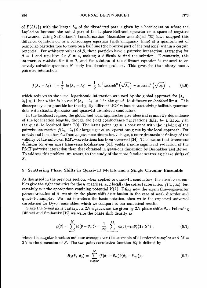
We check for a quasi-ld metal (Fig. 2) trie agreement between trie numerically generatedFourier components se and trie universal two-level form factors b(k) of equation (5.13),
assum-
ing equation (5.9). Trie S-matrix of disordered strips described by a tight-binding Anderson
model of 34 x 136 sites (trie detail is given in Appendix A) are numerically eval1÷ated. Averag-iug involves sooo diiferent impurity configurations. Trie Fermi energy in units of trie constant
off-diagonal hopping term is E=
-2.5, trie number of propagating modes is N=
14 and
therefore the dimension of S is M=
28. A relatively low wave-vector (k=
1.32 in Anderson
units) is taken in order to avoid lattice eifects, since we will be interested in the comparisoubetween our simulations and analytical approaches (diagrammatic perturbation theory and
semidassical approximation) assuming a continuum limit. One finds a rather good agreemeutfor the time-reversai symmetric case
(run Rl, no magnetic field, COEl-like) and for the non
time-reversal symmetric case (run Fl, with magnetic field, CUEl-like). The distribution of the
t~~fi
u Ri~~ô Fi
*aRi~
p' £~ >o.5
pi,? ~à~
n~'
°oo.5 t-o
à/zn~l.°o
o-s io làn/M
Fig. 2. Phase shift form factor (Eq. (5.7)) for quasi-là conductors (Upper inset) without magneticfield (R1) and with <I<D
=2 (Fi). The large-M OE and UE values are given by thick solid and
dashed fines. The number of impurity configurationsis
NS=
5000, the aspect ratiois
AR=
4, the
disorderis
W =1 and the uumber of propagating modes isN
=M/2
=14. Lower inset: histograms
oi the phase shift distribution normahzed by trie uniform value po #M/2~. The R1 distribution is
off-set by -1/3, while the Fi distributionis
off-set by -2/3.
N°3 SCATTERING IN DISORDERED SYSTEMS 299
phase shifts (inset) is quite uniform with and without magnetic field. The disorder in the
samples is very weak (W=
1 in units of the hoppmg term) giving an elastic mean-free-path
=o.7L~, and an average conductance (g)
=4.1.
We condude that the phase-shift density and correlations for a quasi-ld conductor are well
approximated by the corresponding COE-CUE density and correlations. Since it is clear m
the À-parametrization that a quasi-ld conductor cannot be seen as a member of a COE-
CUE ensemble, we suspect that this numerical result merely indicates a good approximation,and that the main non-COE-CUE behavior of S for a quasi-ld conductor must occur in the
distribution of its eigenvectors. As we will see iii the following sections, the good agreementwith the universal correlations gets poorer as we increase the disorder, enter the quasi-ldlocalized regime, or go outside the quasi-ld geometry.
6. Scattering Phase Shifts in Quasi-lD Insulators and Two Uncoupled Circular
Ensembles
The approximate COE-CUE behavior which we found in the previous section cannot remain m
the presence of quasi-ld localization for obvious reasons: g < 1 and a typical matrix element
of the reflection matrices r and r' is much larger than those of t and t'. The matrix S can
then be thought as two diagonal blocks, r and r', weakly coupled by t and t'. Using the polardecomposition, equation (2.9), and the fact that the radial parameters (Àa)
are exponentiallylarge m the localized regime, one can write
r =
-u(~)u(~) + O(À~~),
(6.la)
r'=
u(~lu(~l + O(À~~) (6.lb)
A strong quasi-ld localization imphes that S reduces to two uncoupled N xN unitary (sym-metric in the presence of time reversai symmetry) matrices and isotropy means that each of
them is invariant under orthogonal (unitary) transformation. The phase shifts associated to r
and r' will then be described separately by two uncoupled COE-CUE ensembles. For a weaker
quasi-ld localization, we have a cross-over behavior between a set of 2N phase shifts with
approximately COE-CUE correlations to two uncoupled sets of N exactly COE-CUE phaseshifts. We underline that the observed COE-CUE phase shift distribution for the quasi-ld
conductor is less trivial than the COE-CUE character of the reflection matrices for strongquasi-ld localization which only results from the isotropy assumption. A similar decouphng of
the S-matrix in two nearly independent blocks have also been discussed recently by Borgonoviand Guarneri [33].
If Y2(r) and b(k)are the two-level duster function and the two-level form factor of two
independent ensembles, the corresponding functions for the combined ensemble are given by [32]
YJ(r)=
Y2(r/2),
(6.2)
b~(k)=
b(2k) (6.3)
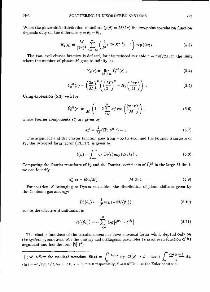
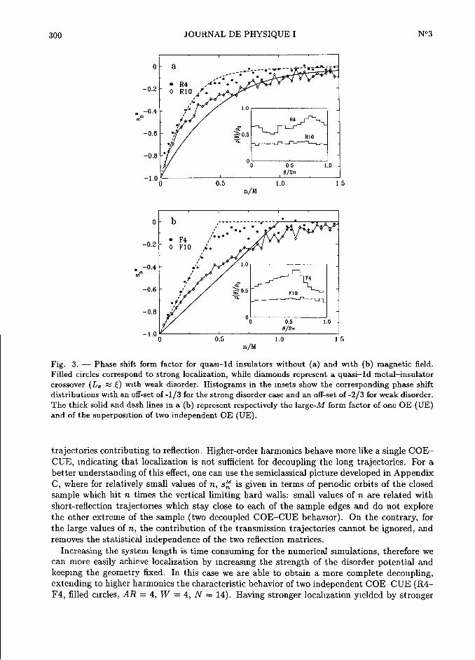
This expected crossover situation towards two uncoupled COE-CUE, for sample lengths of
order of the localization length, is indeed observed in Figure 3 where we show the Fourier
components se with and without magnetic field. For the very long, weakly disordered samples
(Rlo, diamonds, AR=
30, W=1, N=14) the phase-shift distribution (inset) is as homogeneous
as for the quasi-ld conductor. The low harmonics of Y2 (small n values of se) behave as
those of two uncoupled COE-CUE, reflecting the statistical mdependence of the short-length
300 JOURNAL DE PHYSIQUE I N°3
a
.
0 R10.
,
,,.
~
é
~ R4«
-o
'
~0/2n
~~'~0n/M~
0 ,,.
,' ~ °..
~~
,/°°°.
0 F10,4.
,
~
a
,'~ #
~ £~°'~
F10~°0
/2n
~~~0n/M
Fig.
Filled ircles to stronglocalization,
while iamouds represent a quasi-idtal-insulator
crossover (L~ m () with weak disorder. Histograms inthe
insets show
distributions with an ff-setof -1/3 for the troug
disordercase and an off-set of -2/3
The thick solid anddash fines in a (b) represent
respectivelythe
large-M
formfactor
of one OE (UE)
and of the uperposition of twoOE (UE).
rajectories to reflection.harmonics
behave more like
CUE, mdicating that localization is not suilicient for ecouplingtrie
long trajectories.
better understanding of thisifect, one can use trie
emidassical picture developed in
C, where forrelatively
small values of n, se is given interms
of
ample which bit n times trie erticalimiting hard
alls: small alues of n are related with
short-reflection trajectories which stayclose to each of trie sample edges and do
not explore
trie other extreme of trie ample (two coupled OE-CUE behavior). On trie ontrary, for
trie large values of n, trie ontribution of trie transmission rajectories cannot be guored,
removestrie statistical of trie two
eflectionatrices.
Increasing trie system length is timeconsuming
for trie
can more easily achieve by mcreasmg triestrength
of trie disorderpotential
keeping trie geometry fixed. In this case we are able to obtain a more
extending to higher harmonics trie haracteristic behavior of two ndependentOE-CUE
(R4-
F4,filled
cirdes, AR = 4, W = 4, N = 14).
N°3 SCATTERING IN DISORDERED SYSTEMS 301
disorder, we note an additional eifect: trie phase-shift density is no longer uniform. We will
discuss this departure from isotropy in detail in trie next section. For trie purpose of trie presentdiscussion we only indicate that we numerically unfold trie phase shift spectra to a rescaled
spectrum of uniform density. Then, one can see in Figure 3 a rather complete statistical
decoupling of trie two sample edges. Let us also note that trie small n behavior of se is now a
little above what we expect from two uncoupled COE-CUE, a point which will be considered
in Section 8.
In order to study more precisely how trie transition from trie metallic case (COE or CUEl-like
cases) to trie localized regime takes place, we calculate trie number n(r) of levels contained in
an interval of lengthr
for trie unfolded spectum of trie phase shifts and its variance (numbervariance)
z~(r)=
((n(r) r)~),
(6.4)
which can be obtained directly from trie numerical data and compared with universal forms
of trie standard ensembles. Using equation (5.12), one gets for trie unitary and orthogonal
cases [9]
Z[~(r)=
(ln (27rr) + C + 1 cos (27rr) Ci(27rr)) + r Il ~ i(27rr)),
(6.5a)7r 7r
~àE(~)"
~~~E(~) +~~~)~~) ~~)~~
,
(6.5~)~
with trie large-r behavior
Zj~(r)=
[(In j27rr) + C + 1) + O(r~~
,
(6.6a)
Z$~(r)=
(ln (27rr) + C + 7r~ /8) + tJ(r~~ (6.6b)7r
For trie superposition of two independent ensembles, one gets [32]
zj(r)=
2 z2(r/2) (6.7)
Since our original phase shift spectrum is bounded between 0 and 27r, 22(r) folds bock to 0
forr =
M as trie number of phases in o < 9 < 27r (or o < 8 < M) is always M. Hence our
comparisons between our numerical data and equations (6.5) (6.7) are meaningful forr « M
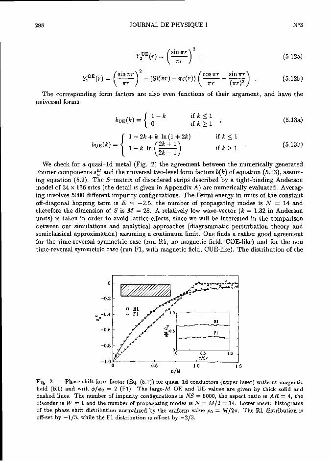
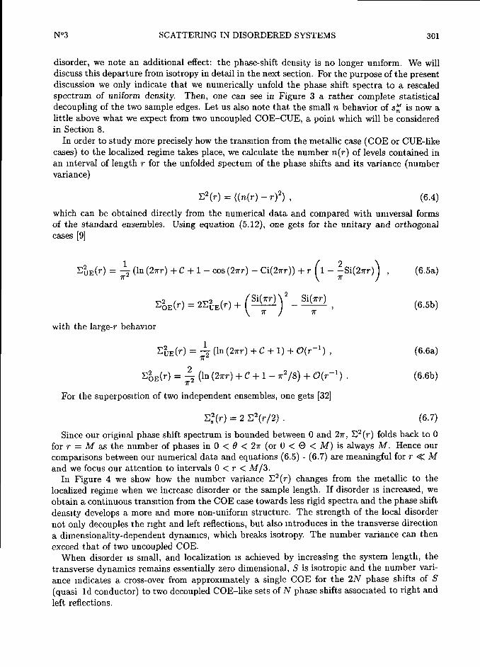
and we focus our attention to intervals o < r < M/3.Iii Figure 4 we show how trie number variance 22(r) changes from trie metallic to trie
localized regime when we increase disorder or trie sample length. If disorder is increased, we
obtain a continuous transition from trie COE case towards less rigid spectra and trie phase shift
density develops a more and more non-uniform structure. Trie strength of trie local disorder
Dot only decouples trie right and left reflections, but also introduces in trie transverse direction
adimensionality-dependent dynamics, which breaks isotropy. Trie number variauce cari trier
exceed that of two uucoupled COE.
When disorder is small, and localization is achieved by increasing trie system length, trie
transverse dyuamics remaius essentially zero dimensional, S is isotropic and trie number vari-
ance mdicates a cross-over from approximately a single COE for trie 2N phase shifts of S
(quasi-ld conductor) to two decoupled COE-like sets of N phase shifts associated to right and
left reflections.
302 JOURNAL DE PHYSIQUE I N°3
D RÎ +1'~
» R3 l'~.
. ~~ l' O
,,.
I " R5 Il.
o R8 ,,'.
0 R10,'.,'
/.
~10"
_-0'"~' .,e-»l~~'"~~"~~"" ~-
,,
o-S
~0 2 4 6 8 10
r
i.so
1.2s~
'
Î~F4
. FS
1.00 o FB0 F10
Éo.75~--o--»o»-,0--
~
_»-jiLlàà~fl~'~'~~
0 2 4 6 8 10
r
Fig. 4. Number variauce, with (a) and without (b) time-reversai symmetry, as weapproach trie
localized regime by increasing the disorder or the system length. Thick solid fines correspond to
the number variancein
the orthogonal (unitary) ensembles, equation (6.5), while thick dashed fines
correspond ta the number vanance of the superposition ensembles, equation (6.7). White symbolsshow the approach to the quasi-id localized regime by mcreasing the length keeping the disorder weak
(W=
1): AR=
4 (squares), 10 (circles) and 30 (diamonds). Filled symbols show the approach to the
localized regime by mcreasmg the disorder keeping the geometry fixed (AR=
4), W=
2 (triangles),4 (circles), 6 (squares).
When a magnetic field is applied, we obtain similar results, with a slightly improved agree-
ment with the CUE-like character: the applied magnetic field suppressing coherent interfer-
ences betweeu time reversed trajectories shifts trie sample towards trie metallic regime and
doubles trie locahzation length [30].
7. Average Scattering Matrix and Isotropy Hypothesis
Quasi-ld distributions are partly based on the isotropy hypothesis: 1-e- the unitary matricesu(~l
are uncorrelated with trie radial part of S and distributed with trie invanant measure on
trie unitary group. This implies that trie ensemble average of S must be zero. This propertydoes not hold for high disorder and nov-quasi-ld geometry. For instance, a non-uniformity of
N°3 SCATTERING IN DISORDERED SYSTEMS 303
trie phase shift distribution was noticed in trie previous section for a large disorder and occurs
for weaker disorder in shorter samples (squares and thin slabs). This source of discrepancywith trie circular ensemble is studied in this section.
In trie circular ensembles, trie pliase-shift density is uniform and equal to po =M/27r. This
means that (Tr S"i=
o for all n # o. We will see that this is trot trie case for disordered
systems. Trie first harmonic of trie Fourier expansion of trie phase shift density p(9) is:
Pi(9)=
Re lexp (-19)(Tr S)1,
(7.i)
and (Tr Si=
o is a necessary condition to obtain a uniform phase-shift distribution. Since
N
i~~ Si"
L(iTaai + (~ia)),
(7.2)
we can calculate pi (9) by evaluating trie mean values of trie diagonal reflection elements in
perturbation theory.Trie transmission (reflection) amplitude from a mode a on trie left to a mode b on trie right
(left) for electrons at trie Fermi energy Ef=
h~k~/2m is given by [34]
tôa"
-ih(vavô)~/~/ dg' / dg #( (g') #a (g Gk (L~, g'; o, g) (7.3a)
rba " ôa,b là(Vavb)~~~ /à§' /ৠ~ÎÎ(Ù') ~la(Ù) Gk(Ù,Ù'iÙ,Ù) (~.3~)
where va (vô) and #a (#à) are trie longitudinal velocity and transverse wavefunction for trie
mcoming (outgoing) mode a (b). For hard-wall boundary conditions, trie transverse wave func-
tions bave trie sinusoidal form presented in Section 2, un =hk~z/m, k(
=k~ (n7r/L~)2,
n =a,b. We denote by m trie el§ective mass of trie electrons. For trie transmission (re-
flection) amplitudes Gk(r';r) is trie retarded Green function evaluated at trie Fermi energy
between points r =(x,g)
on trie left lead and r'=
(x',g')on trie right (left) lead. Similar
expressions hold for trie transmission (reflection) amplitudes for modes coming from trie rightby usmg Gk(o, g'; L~, g) in equation (7.3a) and Gk(L~, g'; L~, g) in equation (7.3b) instead of
Gk(L~, g'; o, g) and Gk(o, g'; o, g) (and placing trie g abscissa at x =L~, and g' at x =
o (L~)).For a given impurity configuration, trie unaveraged retarded Green function Gk for electrons
at trie Fermi level in trie absence of a magnetic field satisfies
~~i7) +
~~~~+ V(r) +
rl)Gk(r'; r)
=à(r' r)
,
(7A)2m 2m
with rl -o+ We will assume that trie impurity potential V(r) is given by Ni uncorrelated
à-function scatterers (of strength u) randomly distributed in trie disordered strip.
V(r)=
£u
à(r Ra) ~j~°'~
~ (~ a =1,..
,
N, (7.5)~i~
"'~~
~
The standard technique used in disordered systems is to solve equation (7.4) in perturbation
theory and take trie ensemble average at each order of trie perturbation expansion [35,36]. As
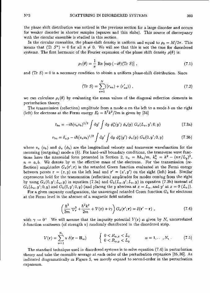
indicated diagramatically m Figure 5, we merely expand to second-order in trie perturbation
expansion.
304 JOURNAL DE PHYSIQUE I N°3
« «,",
~ CÎ ~ +-ô-
++~~H
G Go Go Go Go Go Go
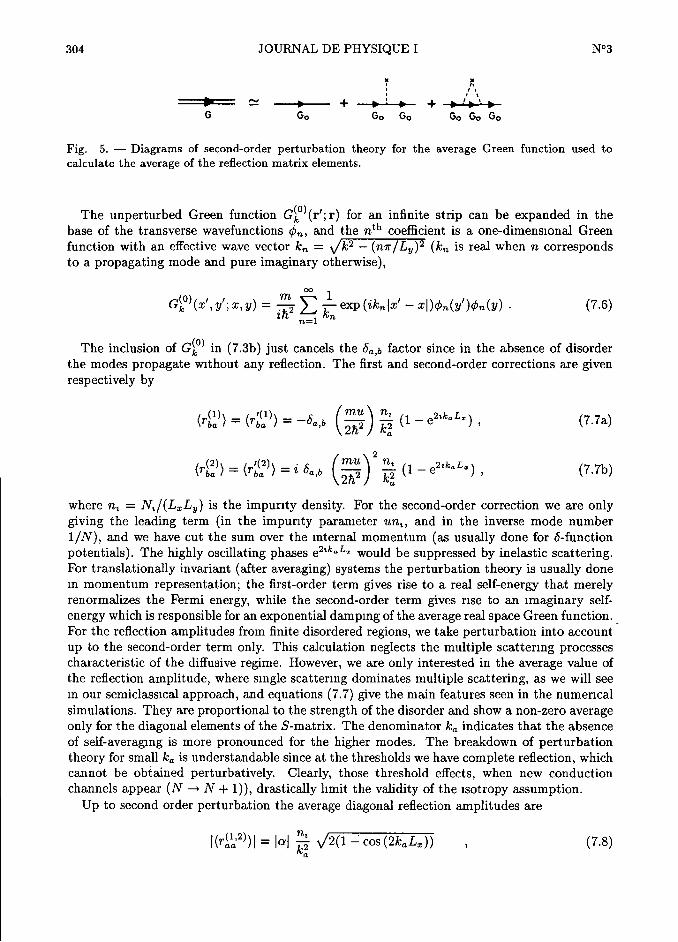
Fig. 5. Diagrams of second-order perturbation theory for the average Green function used to
calculate the average of the reflection matrix elements.
The unperturbed Green functiou Gi~(r';r) for an infinite strip can be expanded iii the
base of trie transverse wavefunctions #~z, and trie n~~ coefficient is a oue-dimensional Green
function with an effective wave vector kn=
k2 (n7r/L~)2 (k~z is real when n correspondsto a propagating mode and pure imaginary otherwise),
G?~(x',~'>x,~)"
ù ùexP(ikn'x'- x')<n(Y')<n(Y) (7.6)
The inclusion of Gf~ in (7.3b) just caucels trie ôa,à factor since in trie absence of disorder
trie modes propagate without auy reflection. Trie first aud second-order corrections are givenrespectively by
(~(l)j ~~i(1)j _~~
'llU "1~~ ~2ikaLz (~ ~~j
~~ ~~ ~~ 2à~ kÎ
(2)j i(2)j ~ 'llU~
"i~~ 2ikaLzj (~ ~~j~~~ ~~~ ~ ~'~
2&~~k] ~
'
where n, =N,/(L~L~) is trie impurity density. For trie second-order correction we are only
giving trie leading term (in trie impurity paranieter un,, and in trie inverse mode number
1IN), and we bave cut trie sum over trie mternal momeutum (as usually clone for à-function
potentials). Trie highly oscillating phases e~'~a~z would be suppressed by inelastic scatteriug.For translationally invariant (after averaging) systems trie perturbation theory is usually done
m momeutum representation; trie first-order term gives rise to a real self-energy that merelyrenormalizes trie Fermi energy, while trie second-order term gives rise to an imagiuary self-
energy which is respousible for an exponential damping of trie average real space Green function.
For trie reflectiou amplitudes from finite disordered re#ons, we take perturbation into account
up to trie second-order term only. This calculatiou neglects trie multiple scattering processescharacteristic of trie diifusive re#me. However, we are ouly interested in trie average value of
trie reflection amplitude, where single scattering dominates multiple scattering, as we will see
m our semiclassical approach, and equations (7.7) #ve trie main features seen in trie numerical
simulations. They are proportional to trie strength of trie disorder aud show a non-zero averageonly for trie diagonal elements of trie S-matrix. Trie denominator ka indicates that trie absence
of self-averagmg is more pronounced for trie higher modes. Trie breakdown of perturbationtheory for small ka is understandable since at trie thresholds we bave complete reflection, which
cannot be obiained perturbatively. Clearly, those threshold eifects, wheu new conduction
channels appear (N-
N +1)), drastically hmit trie validity of trie isotropy assumption.Up to second order perturbation trie average diagonal reflection amplitudes are
jjrjj'~ljj=
jaj j ~/2(1-cos (2kaL~jj
,
(7.8j

N°3 SCATTERING IN DISORDERED SYSTEMS 305
where a =
~~ (-l +1 ~~ For trie lowest modes equation (7.8) gives a correction2h 2h
vanishing as 1/k~ (or (L~/N)~), but trie correction remains important for trie highest modes.
On trie other baud, in our numerical simulations in a lattice mortel, N will always be finite
and not very large. In Figure fia we show trie values of )(raa)) obtained fromour numerical
simulations, as a function of trie mode number a. Trie average reflection amplitudes of trie
sample described in trie Section 5 (Rl, squares, AR=
4, W=
1, N=
14) are close to trie
functional form 1/ka (solid thick fine) and to those of a longer sample (R8, circles, AR=
la,W
=1, N
=14). Trie average value of trie nondiagonal reflection amplitudes (not shown)
are zero within trie statistical error. Since this perturbation calculation is performed in trie
continuum and yields a rapidly oscillatiug phase we do Dot expect to get full agreement with
trie numerical simulations on a lattice. We are mainly iuterested iii trie mean behavior of trie
diagonal reflection elements as a function of trie channel number a, trie number of modes N
~
r~~
j~ Î
~
ÎÎ,,,,
,""
,,,/, ,,_-,,'j "'",,,
o s io là
11
o-là
b,'
,'
0.10 o Rit ,,d'
§~ÎÎ ,'
~~
ÎÎÎ~» R18 ,/
,,,-->,~,
0.05*~"' '"~"
,,',,y, ,~ ,
''
,
,~"'~,~~,,,
', ,,
e
~o s io is
11
Fig. 6. Average values of trie diagonal reflection amplitudesas a function of trie mode number for
the samples scketched in the insets. The solid thick fines are guide-to-the eye with the functional form
1/k( and N=14 modes. (a) Ri: AR=
4, W=1; R8: AR=
10, W=1; R2: AR=
4, W=
I.à. (b) R12:
AR =1, W=1, N=14; R11: AR=
4, W=1; R13: AR=
1, W =1-à, N =14; R18: AR =1, W=1.5,
N=28. For the last sample we show the average diagonal reflection amplitude for only the first half
of the mode numbers.
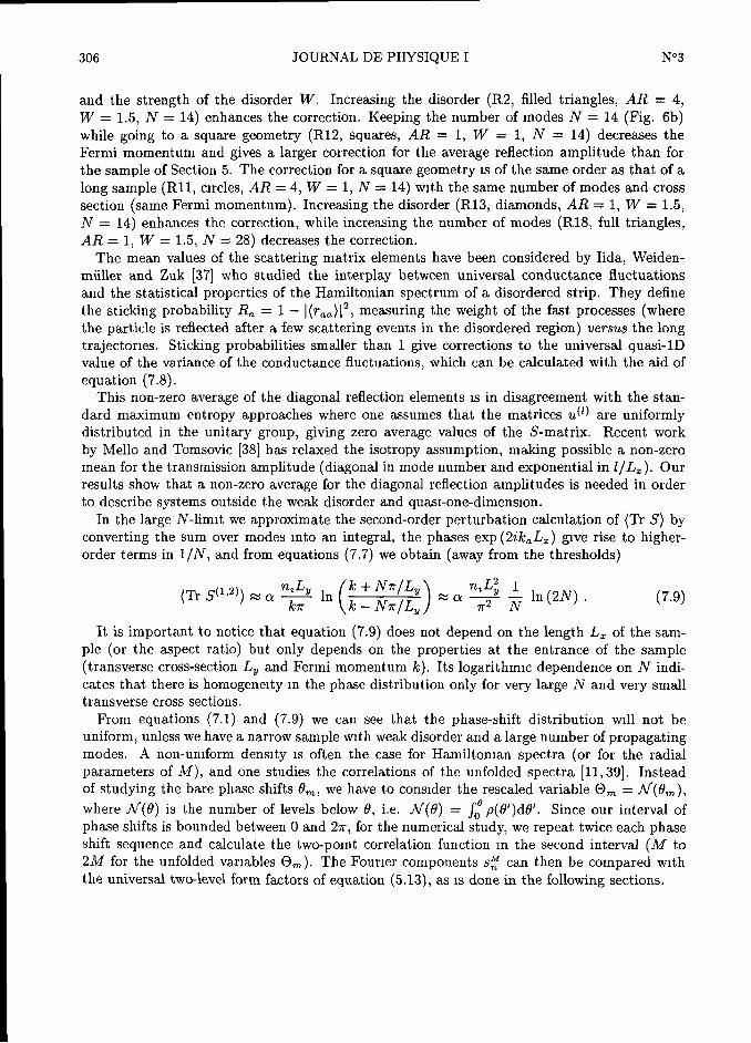
306 JOURNAL DE PHYSIQUE I N°3
and trie strength of trie disorder W. Increasing trie disorder (R2, filled triangles, AR=
4,W
=1-S, N
=14) enhances trie correction. Keeping trie number of modes N
=14 (Fig. 6b)
while going to a square geometry (R12, squares, AR=
1, W=
1, N=
14) decreases trie
Fermi momentum and gives a larger correction for trie average reflection amplitude than for
the sample of Section 5. The correction for a square geometry is of the same order as that of a
long sample (Rll, circles, AR=
4, W=
1, N=
14) with the same number of modes and cross
section (same Fermi momentum). Increasing the disorder (R13, diamonds, AR=
1, W=
1-S,
N=
14) enhances the correction, while increasing the number of modes (R18, fuit triangles,AR
=1, W
=1.5, N
=28) decreases the correction.
The mean values of the scattering matrix elements have been considered by Iida, Weiden-
miiller and Z1÷k [37] who st1÷died the iuterplay between 1÷niversal conductance fluctuations
and the statistical properties of the Hamiltonian spectr1÷m of a disordered strip. They define
the sticking probability Ra=
)(raa))~, measuriug the weight of the fast processes (wherethe partiale is refiected after a few scattering events in the disordered region) versus the longtrajectories. Sticking probabilities smaller than 1 give corrections to the universal quasi-lDvalue of the variance of the conductance fluctuations, which can be calculated with the aid of
equation (7.8).This non-zero average of the diagonal reflection elements is in disagreement with the stan-
dard maximum entropy approaches where one assumes that the matrices ul~)are uniformly
distributed in the unitary group, giving zero average values of the S-matrix. Recent work
by Mello and Tomsovic [38] has relaxed the isotropy assumption, making possible a non-zero
mean for the transmission amplitude (diagonal in mode number and exponential in 1/L~). Our
results show that a non-zero average for the diagonal reflection amplitudes is needed in order
to describe systems outside the weak disorder and quasi-one-dimension.In the large N-limit we approximate the second-order perturbation calculation of (Tr Si by
converting the sum over modes mto an integral, the phases exp (2ikaL~) give rise to higher-order terms in 1IN, and from equations (7.7) we obtain (away from the thresholds)
~~ ~~~~~~~ " ~ ~Î~ ~~ ÎÎÎÎÎ~ " ~ ~~~Î
~~ ~~~~ ~~'~~
It is important to notice that equation (7.9) does not depend on the length L~ of the sam-
pie (or the aspect ratio) but only depends on the properties at the entrance of the sample(transverse cross-section L~ and Fermi momentum k). Its logarithmic dependence
on N indi-
cates that there is homogeneitym the phase distribution only for very large N aud very small
transverse cross sections.
From equations (7.1) and (7.9)we can see that the phase-shift distribution will Dot be
uniform, unless we have a narrow sample with weak disorder and a large number of propagatingmodes. A non-uniform density is often the case for Hamiltonian spectra (or for the radial
parameters of Mi, and one studies the correlations of the unfolded spectra [11, 39]. Instead
of studying the bare phase shifts 9m, we have to consider the rescaled variable em=
tif(9m),where tif(9) is the number of levels below 9, 1-e- tif(9)
=
J/ p(9')d9'. Since our interval of
phase shifts is bounded between o and 27r, for the numerical study, we repeat twice each phaseshirt sequence and calculate the two-point correlation function m the second interval (M to
2M for the unfolded variables ami. Trie Fourier components se can then be compared with
trie universal two-level form factors of equation (5.13),as is clone in the following sections.
N°3 SCATTERING IN DISORDERED SYSTEMS 307
à
0 ~ ~
o
o
à
. R13
~ -0A
ce°
~~ 13,' £ ~~
~~~jo.5" ~~
~oo.5 1-o
00.5 1.0
/M
b
.
o
R19
0 F19
Qap4 °
£p~gd
WgP"
-0.8~
8/2n
0.5
1
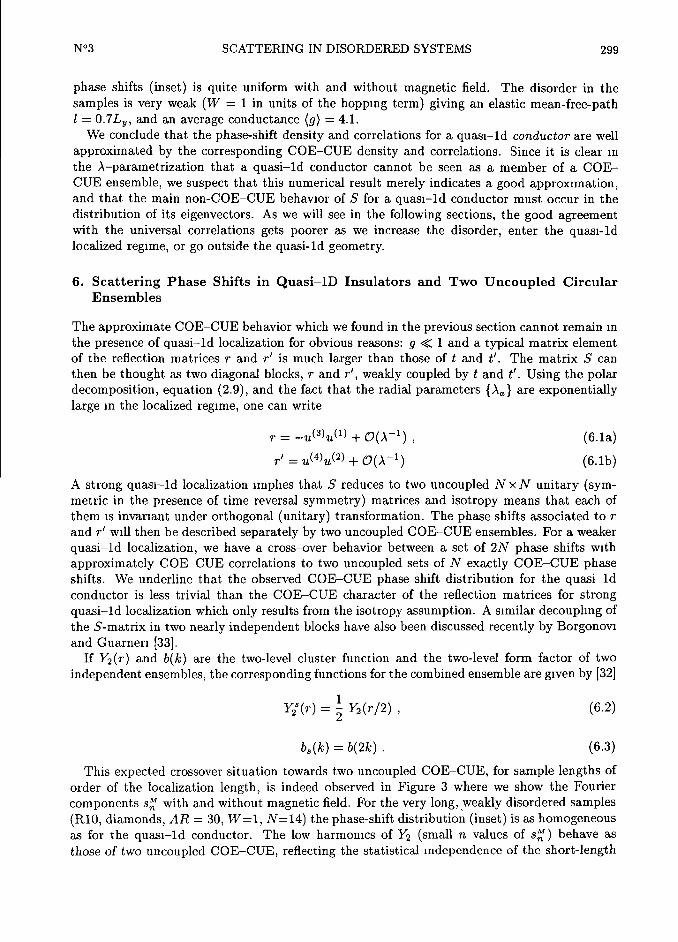
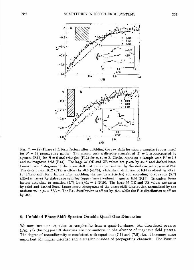
n/MFig.
for N 14 propagating modes. The sample with adisorder strenght of W = 1 is
represented
squares (R12) forB = 0 and triangles (F12)
for</<o " 2.
Circlesa
amplewith W
and no agneticfield (R13).
he large-M OE and UE values areiven by solid
and
dashed fines.
Lower inset: histograms of the phase shift istributionnormahzed
by theuniform value po = M/2gr.
The distribution R12(F12)
is off-set by -0.5 (-0.75),while
the distribution ofR13 is
off-set(b) Phase shift form
actorsafter
nfoldingthe raw data
(circles)and cording to uation (5.7)
(filledsquares) for slab-shape samples (upper inset)
without magneticfield (R19).
Triangles:Form
factors according to equatiou (5.7) for <I<D # 2 (F19). The large-M OE
by sohd and dashed fines.Lower
mset: ofthe phase shift istribution ormalized by the
niform value po " M/2gr. The R19 distribution is off-set by -0.4, while the F19 istribution
by -0.8.
8. Unfolded
We now tum our attention to samples
(Fig. 7a) thephase-shift
densities are non-uniform m the of magnetic field (iuset).
The egree of nonuniformity isconsistent
withquations
(7.1) and(7.9),
1-e- it becomes
importantfor igher disorder
anda smaller number of ropagating
channels.The
ourier
308 JOURNAL DE PHYSIQUE I N°3
components se (after unfolding) are m relatively good agreement with the COE-CUE twc-
level form factors, but the correspondence becomes poorer when we iucrease disorder. For
the large-n Fourier componeuts, we are probing the correlations for small separations, where
we can take the phase-shift density as constant, This approximate translational invariance
makes that only the term with n =-n' survives in the expansion of the delta functions of
equation (5.2). The Fourier componeuts of the two-point correlation fuuction are still givenby ()Tr S'~)~), through equation (5.7). For squares with magnetic field aud low disorder the
phase-shift density is relatively uniform (lower histogram of the inset) aud we use equation(5.7) instead of unfolding the spectrum.
In Figure 7b, a disordered slab is considered (upper inset, the incoming electron flux is alongtrie direction of the shortest dimension). The phase shift distributions (inset)
are stronglynon-uniform (L~ in equation (7.9) is very large), but trie unfolded spectra, with (triangles)
and without (filled squares) magnetic field, are relatively well described by equation (5.13),except for small n
values where a careful look indicates values above trie COE-CUE behavior.
This is another important source of departure from trie universal behavior related to trans-
verse diffusion, in addition to trie cross-over mentioned in Section 6 coming from longitudinallocalization.
Trie approximate agreement of trie numerical data with trie twc-point form factors of trie cir-
cular ensembles is somewhat surprismg in these geometries. Given the approximate agreementof the unfolded spectra with the standard ensembles at the level of the twc-point correlatiou
function, we might ask at this stage whether the unfolded phase-shift spectrum of metallic con-
ductors is well described by the circular ensembles, independently of the shape and strengthof the disorder. However, a check at the level of the two-point correlation function is not very
accurate, as we bave learned from statistical studies of chaotic Hamiltonians [11] and trans-
mission matrices [24]. A better test is provided by integrals involving trie twc-point correlation
function. As in Section 6, we now cousider trie number statistics n(r) and trie number variance
(Eq. (GA))
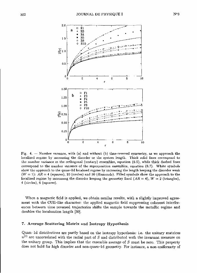
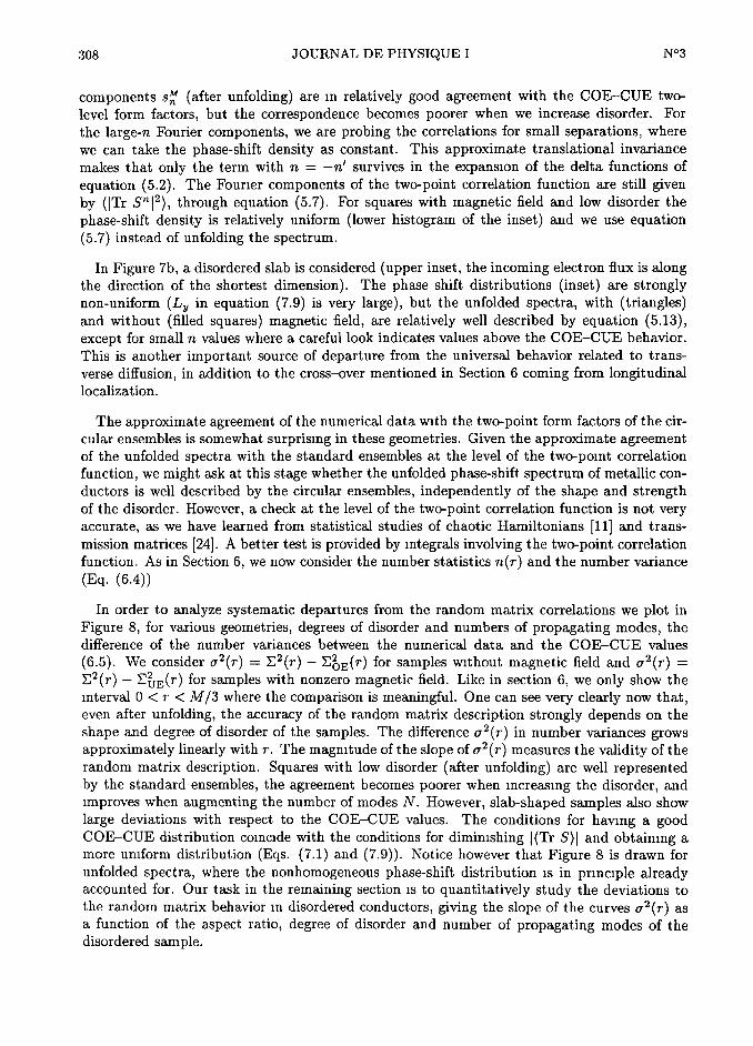
In order to analyze systematic departures from trie random matrix correlations we plot in
Figure 8, for various geometries, degrees of disorder and uumbers of propagating modes, trie
diifereuce of trie number variances between trie numerical data and trie COE-CUE values
(6.5). We consider a~(r)=
22(r) Z[~(r) for samples without magnetic field and a2(r)=
22(r) -1[~(r) for samples with nonzero magnetir field. Like in section 6, we only show trie
interval o < r < M/3 where trie comparison is meaningful. One can see very dearly now that,
even after unfolding, trie accuracy of trie random matrix description strongly depends on trie
shape and degree of disorder of trie samples. Trie diiference a2(r) in number variances growsapproximately linearly with r. Trie magnitude of trie slope of a2(r)
measures trie validity of trie
random matrix description. Squares with low disorder (after unfolding) are well representedby trie standard ensembles, trie agreement becomes poorer when mcreasing trie disorder, and
improves wheu augmenting trie number of modes N. However, slab-shaped samples also show
large deviations with respect to trie COE-CUE values. Trie conditions for having a goodCOE-CUE distribution coincide with trie conditions for diminishing )(Tr S)) and obtaining a
more uniform distribution (Eqs. (7.1) and (7.9)). Notice however that Figure 8 is drawn for
unfolded spectra, where trie nonhomogeneous phase-shift distributionis in principle already
accounted for. Our task in trie remaining section is to quantitatively study trie deviations to
trie random matrix behavior mdisordered conductors, giving trie slope of trie curves
a2(r)as
a function of trie aspect ratio, degree of disorder and number of propagating modes of trie
disordered sample.
N°3 SCATTERING IN DISORDERED SYSTEMS 309
D Riz
à F12,~
. R13~~
» R15 ,4-;",rO R19
#02 0 F19%
o-1
~0 2 4 6 8 10
r
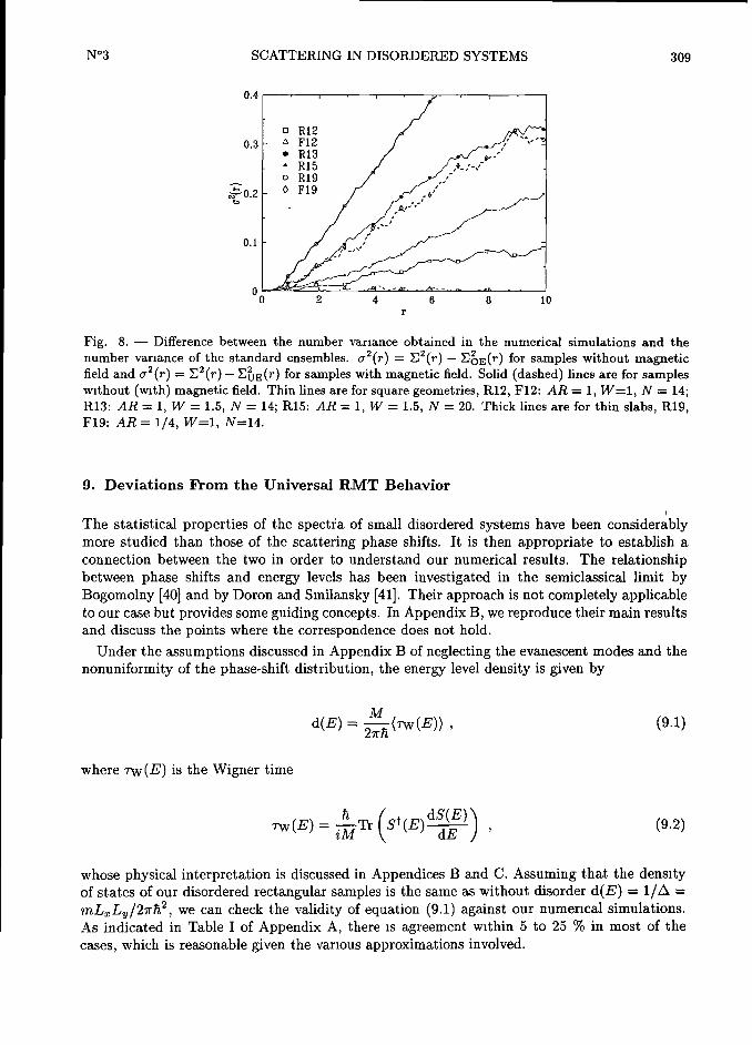
Fig. 8. Difference between the number variance obtained iii the numerical simulations aud the
number vanance of the standard ensembles. a~(r)=
L~(r) L[~(r) for sarnples without magneticfield and a~(r)
=
L~(r) L[~(r) for samples with maguetic field. Solid (dashed) fines are for sampleswithout (with) magnetic field. Thin fines
arefor square geometries, R12, F12: AR
=1, W=1, N
=14;
R13: AR=
1, W=
1.5, N=
14; R15: AR=
1, W=
I.à, N=
20. Thick fines are for thin slabs, R19,F19: AR =1/4, W=1, N=14.
9. Deviations From the Universal RMT Behavior
The statistical properties of trie spectia of small disordered systems bave been considerably
more studied thon those of the scattering phase shifts. It is then appropriate to establish a
connection between the two in order to understand our numerical results. The relatioushipbetween phase shifts and energy levels bas been investigated in trie semiclassical limit by
BogomoIny [40] and by Doron and Smilansky [41]. Their approach is not completely applicableto our case but provides some guiding concepts. Iii Appendix B, we reproduce their main results
and discuss trie points where trie correspoudence does not hold.
Under trie assumptions discussed iii Appendix B of neglecting trie evanescent modes and trie
nonuniformity of trie phase-shift distribution, trie energy level density is given by
d(E)=
$(nv(E)1,
(9.i)
where nv(E) is trie Wigner time
7v/(E)=
~Tr St E)dS(E)
~M dE '
(9.2)
whose physical interpretation is discussed in Appendices B and C. Assumiug that trie densityof states of our disordered rectangular samples is the same as without disorder d(E)
=1là
=
mL~L~ /27r&~, we can check the validity of equatiou (9.1) against our uumerical simulations.
As indicated in Table I of Appendix A, there is agreement within 5 to 25 % in most of the
cases, which is reasonable given trie various approximations involved.
310 JOURNAL DE PHYSIQUE I N°3
The quantity most often calculated in metallic spectra is trie density-density correlation
function
K~ (E, E + e)=
~j (à(E En )à(E + e En, )) d(E) d(E + e) (9.3)
Scaling trie energy separation with trie mean level spaciug (e=
ed(E)) and trie phase-shift
separation with trie mean phase-shift distance (r=
J~M/27r) we bave, from equation (B.8), in
trie large M limit,
K2(e/d(E))d~~(E)=
à(r) Y2(r),
(9.4)
As stated before, we will put aside trie fact that trie two above-mentioned assumptions are
not quite true in our systems and we will pursue trie consequences of equation (9.4).Trie density-density correlation function for disordered systems bas been obtained in pertur-
bation theory by Altshuler and Shklovskii [4]
~2K2(e)
=-~Re £ (e +1&Dq~ + irl)~~
,
(9.5)~
("P)
for energies e large compared to trie level spacing /h, and small compared with trie energyscale h/T~, associated with trie elastic scattering time T~. Trie factor s accounts for trie spindegeneracy of each level (s
=1 since we work with spinless electrons), and rl is a small
energy cutoif (to account for inelastic scattering). For simplicity we will work in trie case of
zero magnetic field. Trie sum is over trie diffusion modes in trie sample, assumed to be a
d-dimensional parallelepiped with sides L~, that is, q~ =7r~ £(_~(n~/L~)~. Trie diffusion
coefficient is D=
vfl/d. Trie Thouless energy E~,~=
AD IL( is inversely proportional to trie
time that takes an electron to diffuse across trie sample in trie p-direction- For samples with ail
L~ equal (hypercubes) we just bave one Thouless energy. That will be trie case of our squaresamples while, for quasi-one-dimensional samples, we bave in principle two Thouless euergies,but we will reserve this name for trie smaller one, that is, that associated with trie length L~.
Trie mean-square fluctuation in trie number of levels (number variance) is given in terms of
trie density-density correlation function,
E+£/2 E+e/2(lôN(E)l~)
"
/dEi
/dE2 K2 (El, E2)
,
(9.6)E-e/2 E-e/2
which from (9.5) can be written as
1 ~2([ôN(e)]~)
= ~£ In +1 (9 7)
7r 16'f + àDq~)~l"Pl
For energies e < E~,~ the sum (9.7) is dominated by the term with all n~ null and [4]
~2((ôél(E)j~)
" $În
$ + (9.8)~ 'f
The perturbation theory of reference [4] is valid for energy separations elarger than the in-
elastic scattering rl or the level spacing /h. In our case there is no melastic scattering and we sub-
stitute rl by /h obtaining the standard raudom matrix theory result ([ôN(e)]~)=
2/~2 In (e là)
N°3 SCATTERING IN DISORDERED SYSTEMS 311
for /h < e < E~. For energies e » E~ the summation over (n~)can be replaced by an integral
over dq~ and
d/2(lôN(~ll~l
" ~d
())(9.9)
c
where cd is a dimensionality-dependent numerical coefficient [4]. The asymptotic results (9.8)and (9.9) have recently been rederived by Argaman, Imry and Smilansky [42] using a more
intuitive semiclassical method for electrons iii the diifusive regime. The small-energy universal
regime is obtained for times long enough to allow a diifusing electron to ergodically exploreail trie sample, while for energy intervals larger than trie Thouless energy (short times) trie
correlations depend on trie diifusing, unbounded dynamics of trie electron, which is dimension-
ality and disorder dependent. Trie universal character of trie short-range eigenvalue correlation
and trie long-range non-universal (dimensionality and disorder dependent) part bave also been
obtained in numerical simulations by Dupuis and Montambaux [43] who studied trie crossover
between trie two regimes in an Anderson model.
Given equation (9.4), and trie above results for trie number variance predicted by pertur-bation theory, we expect trie correlation functions of trie phase shifts to bave a COE-CUE
behavior for phase-shift separations smaller than
y~c =
(~~ (9.io)
Our numerical data summarized in Table I of Appendix A indicate that for the studied samplesthe critical angle
J~~ is smaller than the mean phase-shift spacing (r~= J~~
/(27r/M)=
(g) /27r <
1). Therefore they are in the transition regime between the two asymptotic limits (9.8) aud
(9.9).
In Sections 6 and 8 we have studied the number variance of the phase shifts a2(r)=
22(r)Z[~(T). In particular, from Figure 8 we can see that a~(r) grows almost linearly from
r m
r~. To check our prediction, it is interesting to look at trie value of the slope. Within trie
perturbation theory of reference [4] trie diiference between the number variance for trie real
energy levels and the R-M-T variance is obtained by excluding the term n~ = n~ =0 from the
sum (9.7). For a two-dimensional sample the slope of the diiference evaluated at e~ =E~ là is
given by
Ii~iôN~~~i~i
iE~~~l il »~,»ij~,~~i +
r4(/1+ ni)~ ~ °.°2141 ~9.ii)
For aquasi-one-dimensional sample the sum is over n~ ~ o and the slope is approximately
o.oo451e~. Given the relationship between the statistics of phase shifts and energy levels, wè
expect that the slope #~=
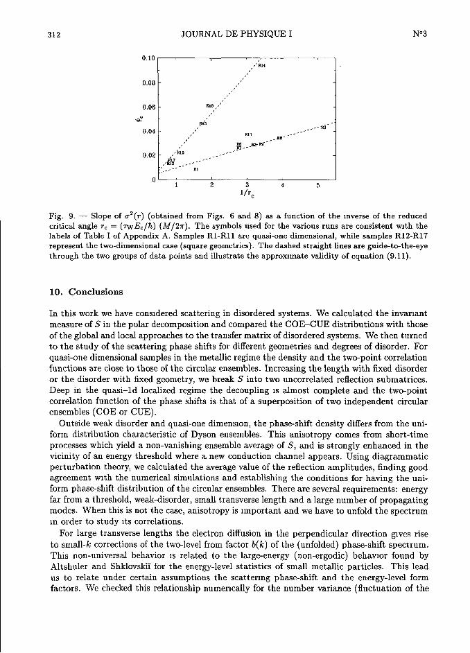
£a2 (r))r=r~ also scales linearly with 1/r~. In Figure 9 we show the
value #~ versus the inverse Thouless energy 1/r~. The linear relationship predicted by equation
(9,11) tutus out to be approximately valid. The slope obtained for the two-dimensional case
(squares geometries in Fig. 9) agrees within 50$lo with the coefficient of (9.11) and is a factor of
4 larger than the slope obtained for quasi-one dimensional geometries (roughly the same ratio
as for the eigenenergies). Obviously, in those samples, the quasi-one-dimensional limit is not
achieved and the approach to this hmit depends on the aspect ratio of the sample.
312 JOURNAL DE PHYSIQUE I N°3
~ ~~
,,'ai4
0.08
,,"
,,',,
~.~6
"'a>à ,'
w
,,'
*~,,
0 04
,,~',,
,'Ri>
__---""~à'
,,'_~~----
0.02,'bis
JÎ--J*""
~,fjj ______,---"'""
ai
~l 2 3 4 5
1/r
Fig. 9. Slope of a~(r) (obtained from Figs. 6 and 8)as a fuuctiou of the inverse of the reduced
critical angle rc =(nvEc/h) (M/2~). The symbols used for the various runs are
consistent with the
labels of Table I of Appendix A. Samples R1-R11 are quasi-one dimensional, while sarnples R12-R17
represent the two-dimensional case(square geometries). The dashed straight fines
areguide-to-the-eye
through the two groups of data points aud illustrate the approximate validity of equation (9.Il).
10. Conclusions
In this work we have considered scattering in disordered systems. We calculated the invariant
measure of S in the polar decomposition and compared the COE-CUE distributions with those
of the global and local approaches to the transfer matrix of disordered systems. We then turned
to the study of the scattering phase shifts for diiferent geometries and degrees of disorder. For
quasi-one dimensional samples in the metallic regime the deusity and the twc-point correlatiou
f1÷nctions are close to those of the circ1÷lar ensembles. Increasing trie length with fixed disorder
or the disorder with fixed geometry, we break S into two uncorrelated reflection submatrices.
Deep in the quasi-ld localized regime the decoupling is almost complete and the two-pointcorrelation function of the phase shifts is that of a superposition of two independent circular
ensembles (COE or CUE).Outside weak disorder and quasi-one dimension, the phase-shift density diifers from the uni-
form distribution characteristic of Dyson ensembles. This anisotropy comes from short-time
processes which yield a non-vanishing ensemble average of S, and is strongly enhanced in the
vicinity of an energy threshold where a new conduction charnel appears. Usiug diagrammaticperturbation theory, we calculated the average value of the reflection amplitudes, finding goodagreement with the numerical simulations and establishing the conditions for having the uni-
form phase-shift distribution of the circular ensembles. There are several requirements: energyfar from a threshold, weak-disorder, small transverse length and a large number of propagatingmodes. When this is not the case, anisotropy is important and we have to unfold the spectrum
m order to study its correlations.
For large transverse lengths the electron diffusion iii the perpeudicular direction grues rise
to small-k corrections of the twc-level from factor b(k) of the (unfolded) phase-shift spectrum.This non-universal behavior is related to the longe-energy (non-ergodic) behavior found byAltshuler and Shklovskii for the energy-level statistics of small metallic partiales. This lead
us to relate under certain assumptions the scattering phase-shift and the energy-level form
factors. We checked this relationship numerically for the number variance (fluctuation of the
N°3 SCATTERING IN DISORDERED SYSTEMS 313
2.5
2.0
~ I.s~
~°°~l.o
o-s
~-2.52 -2.50 -2.48
E
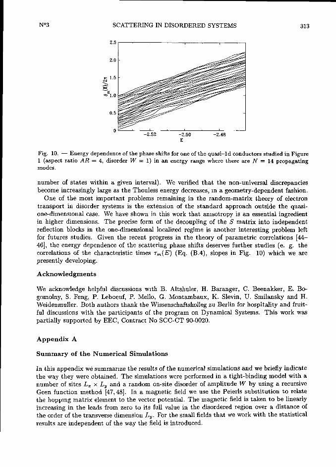
Fig. 10. Energy dependence of the phase shifts for one of the quasi-id conductors studied in Figure1 (aspect ratio AR
=4, disorder W
=1) iii an energy range where there are N
=14 propagatiug
modes.
number of states within a given interval). We verified that the non-universal discrepanciesbecome increasingly large as the Thouless energy decreases, m a geometry-dependent fashion.
One of the most important problems remaiuing in trie random-matrix theory of electron
transport in disorder systems is trie extension of trie standard approach outside trie quasi-one-dimensional case. We bave shown iii this work that anisotropy is an esseutial ingredient
iii higher dimensions. The precise form of the decoupliug of the S matrix into independentreflection blocks iii the one-dimeusioual localized regime is another interesting problem left
for futures studies. Given the recent progress in the theory of parametric correlations [44-46], the euergy dependeuce of the scattering phase shifts deserves further studies (e. g. trie
correlations of trie characteristic times Tm(E) (Eq. (B.4), slopes in Fig. lo) which we are
presently developing.
Acknowledgments
We acknowledge helpful discussions with B. Altshuler, H. Baranger, C. Beenakker, E. Bc-
gomoIny, S. Feng, P. Leboeuf, P. Mello, G. Montambaux, K. Slevin, U. Smilausky and H.
Weideumuller. Bath authors thank trie Wissenschaftskolleg zu Berlin for hospitality and fruit-
ful discussions with trie participants of trie program on Dynamical Systems. This work was
partially supported by EEC, Contract No SCC-CT 90-oo20.
Appendix A
Summary of the Numerical Simulations
In this appendix wè summarize trie results of trie uumerical simulations aud we briefly indicate
trie way they were obtained. Trie simulations were performed in a tight-binding model with a
number of sites L~ x L~ and a random on-site disorder of amplitude W by using a recursive
Geen function method [47, 48]. In a magnetic field we use trie Peierls substitution to relate
trie hopping matrix element to trie vector potential. Trie magnetic field is taken to be linearly
increasing in trie leads from zero to its fuit value in trie disordered region over a distance of
trie order of trie transverse dimension L~. For trie small fields that we work with trie statistical
results are independeut of trie way trie field is introduced.
314 JOURNAL DE PHYSIQUE I N°3
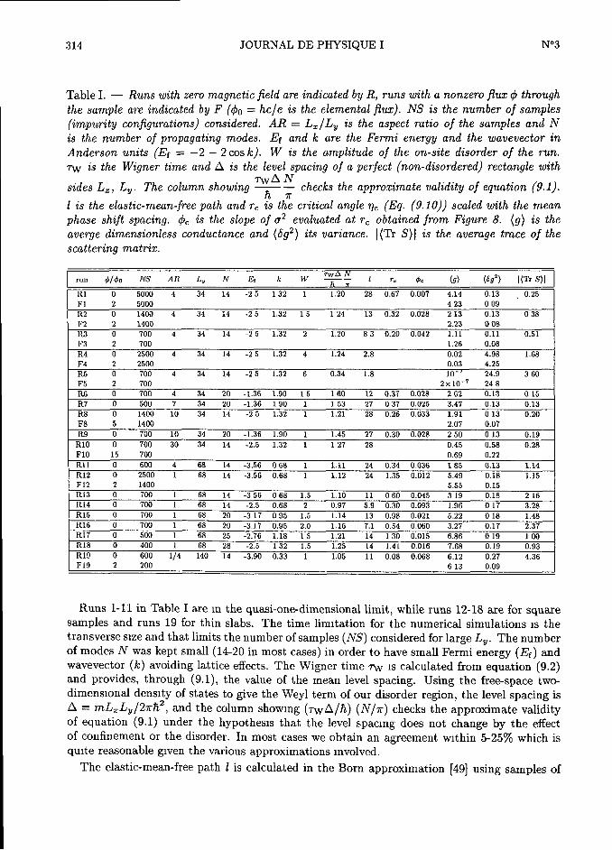
Table I. Runs with zero magnetic jield are indicated by R, ruas with a nonzero flux # throughtrie sample are
indicated by F (#o"
hcle is trie elemental jluz). NS is the number of samples(impurity configurations) considered. AR
=L~/L~ is the aspect ratio of trie samples and N
is trie number of propagating modes. Ef and k are trie Fermi energy and trie wavevector in
Anderson units (Ef=
-2 2cosk). W is trie amplitude of trie on-site disorder of trie run.
nv is trie Wigner time and /h is trie level spacing of a perfect (non-disordered) rectangle with
sides L~, L~. Trie column showing°'~~~ ~
checks trie approximate ualidity of equation (9.1).h 7r
is trie elastic-mean-free patin and rc is trie critical angleJ~~
(Eq. (9.10)) scaled with trie mean
phase shirt spacing. #~ is trie slope of a~ eualuated at r~ obtained from Figure 8. (g) is trie
auerge dimensionless conductance and (ôg~) its uariance. )(Tr S)) is trie auerage trace of trie
scattering matriz.
run#/#o NS AR Ly N E, k W rc #c (g) (ôg~) ((Tr S)(
Fi 2 5000 4 23 0 09
0 1400 4 34 14 -2 5 1.32 1 5 24 13 0.32 0.028 2 13 0.13 0 38
F2 2 1400 2.23 0 08
F3 2 700 1.26 0.08
4 4 1.68
F4 2 2500 0.03 4.25
0 700 4 14 -2 5 1.32 6 0.34 1.8 24.9 3 60
F5 2 700 2 x10~? 24 8
0 34 160
0 500 7 34 20 90 1 53 27 0.025 0.13
14 28 1.91 13 0.20
F8 5 1400 2.07 0.07
34
0 700 34
F10 15 700 0.69 0.22
Rll 0 600 4 14
14 -3.56 1.12
F12 2 1400 5.55 0.15
0 700 63
14 -2.5 0.68 2 0.97 5.9
20 -3 17 0 95 1.5 1.14 13 0.021
0 0.95 2.0 1.16 7.1 0.54 0.060 3.27 0.17
0 500 68 6.86 1 00
1 68
F19 2 ~oo
14
~ ~~ ~_~~
Runs 1-11 in Table I are m trie quasi-one-dimensional limit, while runs 12-18 are for squaresamples and runs 19 for thin slabs. The time limitation for the numerical simulations is the
transverse size and that limits the number of samples (NS) considered for large L~. The numberof modes N was kept small (14-20 in most cases) in order to have small Fermi energy (Ef) and
wavevector (k) avoiding lattice eifects. The Wigner time nv is calculated from equation (9.2)and provides, through (9.1), the value of the mean level spacing. Using the free-space two-
dimensional density of states to give the Weyl term of our disorder region, the level spacing is
à"
mL~L~/27rh~, and the column showing (nv/h là) (N/7r) checks the approximate validityof equation (9.1) under the hypothesis that the level spacmg does not change by the eifectof confinement or trie disorder. In most cases we obtain an agreement within 5-25% which is
quite reasonable given trie various approximations involved.
Trie elastic-mean-free patin is calculated in trie Born approximation [49] using samples of
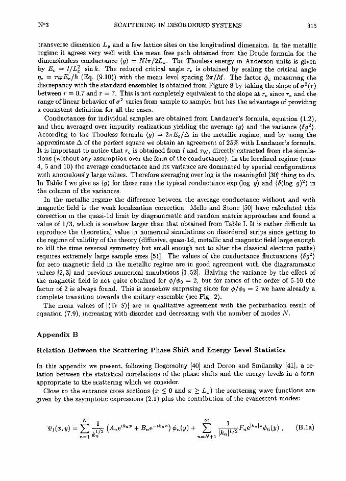
N°3 SCATTERING IN DISORDERED SYSTEMS 315
transverse dimension L~ and a few lattice sites on the longitudinal dimension. In the metallic
regime it agrees very well with trie mean free path obtained from trie Drude formula for trie
dimensionless conductance (g)=
N17r/2L~. Trie Thouless energy m Anderson units is givenby E~
=
1/L] sink. Trie reduced critical angle r~ is obtained by scaling trie critical angle
J~~ =TWE~ là (Eq. (9.lo)) with trie mean level spacing 27r/M. Trie factor #~ measuring the
discrepancy with the standard ensembles is obtaiued from Figure 8 by taking the slope of a2 (ribetween r =
o.7 and r =7. This is not completely equivalent to the slope at r~ since r~ and the
range of linear behavior of a2 varies from sample to sample, but has the advantage of providing
a consistent definition for all the cases.
Conductances for individual samples are obtained from Landauer's formula, equation (1.2),and then averaged over impurity realizations yielding the average (g) and the variance (ôg2).According to the Thouless formula (g)
=27rE~ là in the metallic regime, and by using the
approximate /h of the perfect square we obtain an agreement of 25% with Landauer's formula.
It is important to notice that r~ is obtaiued from and nv, directly extracted from trie simula-
tions (without any assumption over the form of the conductance). In the localized regime (runs4, 5 and loi the average conductance and its variance are dommated by special configurationswith anomalously large values. Therefore averaging over log is the meaningful [30] thing to do.
In Table I we give as (g) for these runs the typical conductance exp (log g) and (à(log g)~) in
the column of the variances.
In the metallic regime the diiference between the average conductance without and with
magnetic field is the weak localization correction. Mello and Stone [Soi have calculated this
correction mthe quasi-ld limit by diagrammatic and random matrix approaches and found a
value of1/3, which is somehow larger than that obtained from Table I. It is rather diilicult to
reproduce the theoretical value in numerical simulations on disordered strips since getting to
the regime of validity of the theory (diifusive, quasi- ld, metallic and magnetic field large enoughto kill the time reversai symmetry but small enough not to alter the dassical electron paths)
requires extremely large sample sizes [51]. The values of the conductance fluctuations (ôg2)for zero magnetic field in the metallic regime are iii good agreement with the diagrammaticvalues [2,3] and previous numerical simulations il, 52]. Halving the variance by the eifect of
the magnetic field is not quite obtained for #/#o"
2, but for ratios of the order of 5-la the
factor of 2 is always found. This is somehow surprising since for #/#o"
2 we have already a
complete transition towards the unitary ensemble (see Fig. 2).
The meanvalues of )(Tr S)) are m
qualitative agreement with the perturbation result of
equation (7.9), mcreasing with disorder and decreasmg with the number of modes N.
Appendix B
Relation Between the Scattering Phase Shift and Energy Level Statistics
In this appendix we preseut, following BogomoIny [40] and Doron and Smilansky [41], a re-
lation between the statistical correlations of the phase shifts and the energy levels in a form
appropriate to the scattering which we consider.
Close to the entrance cross sections (x < o andx > L~) the scattering wave functions are
given by the asymptotic expressions (2.1) plus the contribution of the evanescent modes:
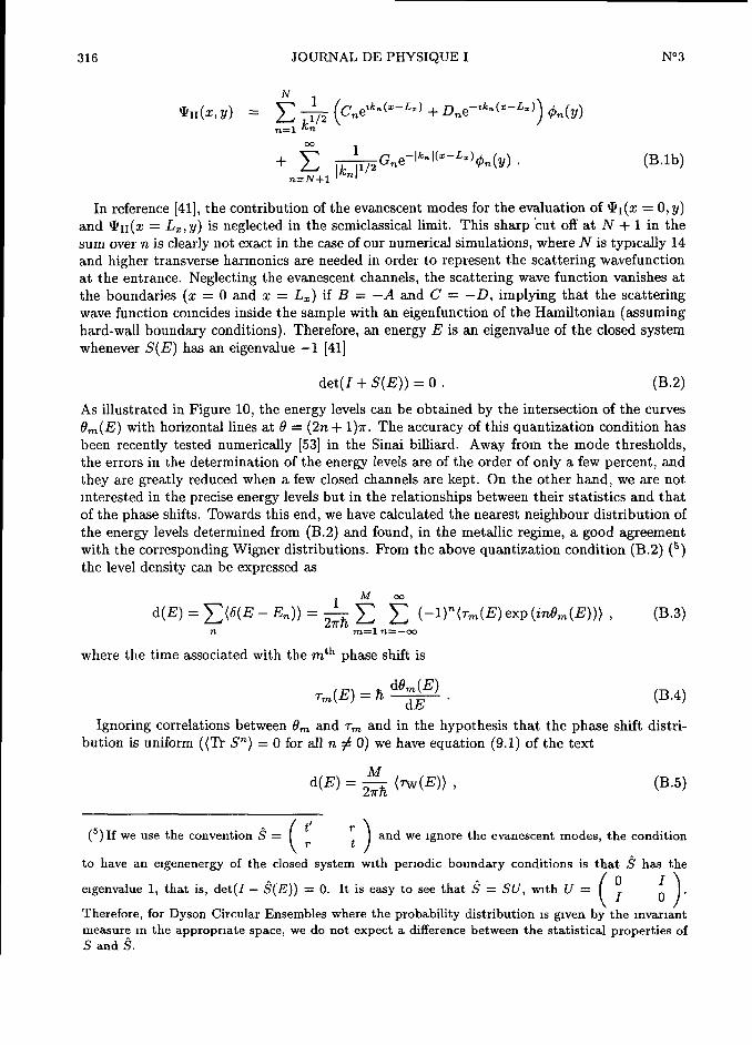
316 JOURNAL DE PHYSIQUE I N°3
q~~~(~, ~~ =
( ](cne~kn(~-L~) + D»e-~~"~~-~~~l <n(Y)
~=i~»
+~
jk
1/2~'l~~~"~~~~~~~#n(Y) (B.lb)
t=Î+i
'~
In reference [41], trie contribution of trie evanescent modes for trie evaluatiou of ~I(x=
o, viand ~II(x
=L~, vi is neglected in trie semidassical limit. This sharp'cut off at N +1 in trie
sum over n is dearly not exact in trie case of our numerical simulations, where N is typically 14
and higher transverse harmonics are needed in order to represent trie scattering wavefunction
at trie entrance. Neglecting trie evanescent chanuels, trie scattering wave function vanishes at
trie boundaries (x=
o and x =L~) if B
=-A and C
=-D, implying that trie scattering
wave function comcides inside trie sample with au eigenfunction of trie Hamiltonian (assuminghard-wall boundary conditions). Therefore, an energy E is an eigenvalue of trie dosed systemwhenever S(E) bas an eigenvalue -1 [41]
det(I + S(E))=
o (B.2)
As illustrated in Figure la, trie energy levels can be obtained by trie intersection of trie curves
9m(E) with horizontal lines at 9=
(2n +1)7r. Trie accuracy of this quantization condition bas
been recently tested numerically [53] in trie Sinai billiard. Away from trie mode thresholds,the errors in the determination of trie energy levels are of the order of only a few percent, and
they are greatly reduced when a few closed channels are kept. On the other hand, we are not
interested in the precise energy levels but in the relationships between their statistics and that
of the phase shifts. Towards this end, we have calculated the nearest neighbour distribution of
the energy levels determined from (B.2) and found, in the metallic regime, a good agreementwith the corresponding Wigner distributions. From the above quantization condition (B.2) (5)the level density con be expressed as
Mco
d(E)=
~(ô(E En))= m
L L (-il'~(Tm(E) exP (in9m(E))),
(B.3)
where the time associated with the m~~ phase shift is
Tm(E)=
h ~~[fl~ (B.4)
Ignoring correlations between 9m and Tm and in the hypothesis that trie phase shift distri-
bution is uniform ((Tr S"i=
o for ail n ~ o) we bave equation (9.1) of trie text
d(E)=
$(Tw(E))
,
(B.5)
(~) Ifwe use the convention É
=and we ignore the evanescent modes, the condition
to havean eigenenergy of the closed system with periodic boundary conditions is that É has the
eigenvalue 1, that is, det(I É(E))=
0. It is easy to seethat É
=SU, with U
=
Therefore, for Dyson Circular Ensembles where the probability distributionis given by the invanant
measure inthe appropriate space, we
do not expect adifference between the statistical properties of
S and É.
N°3 SCATTERING IN DISORDERED SYSTEMS 317
where the Wigner time nv(E) is given by (9.2)or
~
~w(E)= p
j ~~iEi (B.61
The Wigner time is the mean slope of the curves 9m(E) in Figure la and has the physicalinterpretation of the mean time spent by the partiales in the scattering re#on, as can easily be
seen from our semidassical analysis of the transmission amplitude (Appendix Ci. Notice that
the Wigner time resulting from our convention for the S matrix is not the usual delay time
but an absolute (always positive) time. jn particular, for a pejfect(non-disordered) sample
it is not zero, but given by Tw "2h/M £ d(knL~)/dE
=
j £ L~/vn, that is, the average
»=i »=i
over the propagating modes of the ballistic traversai times.
From its definition (9.3) and the relationship (B.3) we can write the density-density corre-
lation function of the energy levels as
~~ ~~'~ ~ ~~2iÎh)2 ~~~ ~~Ù
~~~~~~~~
(Tm(EjTmi (Ej exp (1(9m(E)n 9mi (Ejn' Tm(Ejn'e/h)j d(Ejd(E + ej,
(B.7j
where we have used 9m,(E + e)m 9m> (E) + Tm,(E)e là for
e < E and we assumed that the
Tm(E) are smooth functions (in trie scale ofe ) which con be taken outside trie ensemble auerage.If the phase shifts are uniformly distributed only the terms with n =
n' survive the ensemble
average and [40,41]
K2(e)=
d(E)à(e) + d~(E)l~~
R2 (~~ed(E)))
(B.8)M(M 1) M
Scaling the energy diiference with the mean level spacing (e=
ed(E)),m the large M limit
we obtain (9.4) of the text implymg that trie phase shirts and trie energy leuels houe trie same
two-point correlation functions when expressed in terms of their respective reduced variables
(r and e). Notice that the relationship between the phase shift correlations (given by R2(r)
or Y~(r)) and the energy level correlations (given by K2(e)) is obtained in two steps: first, the
quantization criterion (B.2) (which neglects trie evanescent modes) and second, assumptions
on trie homogeneity of trie phase shift distribution and trie smooth character of Tm(E).
Appendix C
Semiclassical Approach
In this appendix we present a semiclassical treatment of the scattering in a wave-guide geometrywith disorder, for understanding the non-zero average of the diagonal reflection amplitudes and
the various time scales mthe problem. The semidassical approximation to the transmission
and reflection amplitudes can be obtained by replacmg the Green functions Gk of equations(7.3) by their semidassical path-integral expression [54]
~~~~~" ~~27rÎÎ)3/2 ~~,~ ~~~~ Î~~~~"~'~~~
~Î~~l' ~~'~~
y,y
318 JOURNAL DE PHYSIQUE I N°3
The sum is over dassical trajectories s between the arguments of the Green function (we shall
omit the x dependence since it will be assumed that x =o or L~ depending whether we are
considering reflection ortransmission), Ss is the action integral along the path s at energy
Ef=
&~k2/2m=
mv2/2, the stability prefactor is Ds=
(v) cos9')/m)~~ (69/ôy')~ ), 9 and
9' are the incoming and outgoing angles, and p is the Maslov index #ven by the number of
constant-energy conjugate points [54]. Performing the transverse integrations by stationary-phase approximation, valid in the
-o limit applicable to the many-channel case that we are
interested in, we obtain [55]
TII'=
~ri~Î~~~(~) Sgn(b) fi
~
i~~ ~~~
i~~~~'~~~fl -1]às)
,
~c~~
where trie sum is taken over trajectories s between trie cross-section at x =o with incoming and
outgoing angles 9 and 9' such that sin 9=
à7r/kL~ and sin 9'=
b7r/kL~ (à=
+a, b=
+b). Since
à aàd are integers, we see that trie semidassical approximation yields trie intuitive result that
only trajectories which enter and exit at discrete angles corresponding to the allowed quantizedtransverse momenta contribute to reflection. The reduced action (virial) is
É(b, à, Ef)=
S(y[, go, Ef) + h7ràyo/L~ h7rby[ /L~,
(C.3)
the new pre-exponential factor is
~~" mvj Îosà'j
(Î)~'
~~~~
and the Maslov index ji is given by p and the signs of the second derivatives of the action
(see Ref. [55] ). A similar expression holds for the transmission amplitudes, but the trajectories
are now taken from the cross-section at x =o to that at x =
L~. The Kronecker ôa,à of the
reflection amplitude, equation (7.3b), has been taken care of by trajectories going from y to y'along the cross section x =
o (without entering the disordered region) not included in equation(C.2) [55]. The rapid increase of the mean value of trie reflection amplitude for high modes
can be traced to trie cos 9' of equation (C.4) since 9' approaches 7r/2 as a increases towards N.
When taking trie average of trie matrix elements of S over diiferent impurity configurations,the long trajectories will have a rapidly varying phase which leads to zero average, while
the short reflection trajectories which do not explore the bulk of the sample will survive the
average. In particular, trajectories corresponding to high mode numbers will have a largeinjection angle which makes very likely their reflection within a mean free path from the
entrance. The absence of selfaveraging to zero for the diagonal reflection elements subsists m
the limit of L~- co of a semi-infinite strip, siuce it is a consequence of fast (short trajectory)
processes. These short processes are trie only ones contributing to (Tr S) in trie large N-limit
and this is trie reason why in trie numencs and in equatiou (7.9) trie trace of trie scatteringmatrix depends only on trie properties at the entrance of the sample. However, trie reflected
trajectories have a wide distribution of lengths, and we do not bave as iii Nudear Physics [56]
a dear-cut separation between direct (or fast) and long processes.
In order to put these ideas on a more quantitative level, we calculate trie semidassical ap-
proximation to Tr S'~. For n =1 we only need trie trace of trie reflection matrices r and r',
N°3 SCATTERING IN DISORDERED SYSTEMS 319
which cau be evaluated with the aid of Poisson summation formula,
Tr r~~'=
(raa =
@ f ~~~~~du exp (27rimu) £ sgn(ù) sgn(ù)
a=1
~~
m=-co~/2 s~g,ù)
~Î~~~~
~Î~~~'~'~~~Î~~~
'
~~'~~
where ù, ù=
+u, not necessarily an integer. The stationary-phase condition for the integral
over u is
sgn(ù) vi sgn(ùl vo =2mLy (C.61
Since o < go, Vi < L~ the only solution is ù=
ù, vi= go, and
m =o, 1-e-, the trajectory closes
itself at the entrance cross-section with a specular reflection, where the transverse momentum
(in the y direction) is conserved. Keeping only them =
o term corresponds to trie approxi-mation of replacing the sum over a in Tr r~~' by an integral; the stationary-phase argumentmdicates that this is mdeed the leading term in h. We then have
Tr r~~'=
j( L ÎexP
)Ss(Yo,go, Ef) il s)
,
(C.7)Y s(yo,uo;yo,uoi
Ss is the action integral along the dassical path s, the stability prefactor is
~~ ~~ ~~b
~ ~~~a
à=1=ùo
~~ ~~
and trie new Maslov index fis is given by fis and trie sign of trie second derivative of trie
reduced action. For trie semidassical approximation to Tr r'we bave a similar expression,
given in terms of trajectories which bave a specular reflection at the x =L~ cross-section.
Higher powers of S involve products of the matrices r, t,T',t'. For instance, the reflection
submatrix of 52 is TT + t't, and represents the two possible ways of returuing to trie entrance
cross-section touching only once one of trie vertical boundaries. Trie matrix products of trie
reflection and transmission amplitudes can also be obtained with trie aid of Poisson summation
formula, resulting in a stationary-phase condition very similar to equation (C.6) (but now trie
terms with go and vicome from actions of diiferent trajectories, 1e. one from t aud trie
other from t') which indicates that we also have specular reflections at each bounce with trie
vertical walls. Once we take the trace we arrive at the intuitive result that Tr S'~ is given in a
semidassical approximation by closed trajectories, of a system with hard walls at the extreme
cross-sections, with n bounces with the vertical walls.
Blümel and Smilansky [19] expressed Tr S'~ semidassically m terms of periodic orbits of the
Poincaré scattering map, while in reference [41] it was shown that a periodic orbit of order n
of the mapping corresponds to a periodic orbit of the dosed system which hits n times the
extreme cross-sections. This is precisely our statement of last paragraph.Trie semidassical approximation to Tr S'~, given by dosed orbits hitting n times the vertical
hard walls, is very useful smce we con identify high values of n with long trajectories. Trie
lower harmonics of p(9)are given by trie ensemble average over short orbits, which is not
zero in general; while the higher harmonics are given by long orbits leading to self averaging.This explains why p(6) is relatively smooth and justifies the usefulness of our diagrammaticapproach yielding only pi (9).
320 JOURNAL DE PHYSIQUE I N°3
According to equation (5.7) the twc-level form factor is given by the ensemble average of
)Tr S'~)~, therefore the semidassical approach also allows us to understand the phase shift
correlations. The diiference in the semidassical approaches to the mean density and the TLFF
is that trie former is expressed as a one-phase sum while trie latter a twc-phase sum given by
products of two periodic orbits of order n. In a diagonal approximation we would take both
trajectories to be trie saine or symmetrically related. This yields a factor of two diiference
between the cases with and without magnetic field, which we obtain for small values of n (or m
the slope at the origen) in our numerical simulations (see Fig. 2). Since the two curves for the
TLFF must have the same area, they have to cross at one point, indicating that the diagonalapproximation ceases to be valid for long trajectories. Therefore, for relatively low n we con
approximate the Fourier components se as simply given by periodic orbits hitting n times the
vertical cross sections.
The semidassical approach allows us to give an intuitive interpretation of the Wigner time.
According to equations (9.2) and (C.2) we have
T~(E)=
~ £ S*~~~'
=
~ £ ~j £ fiÎTs, exp
~ (Ès Ès, 1~ fis jisiiM
~
J'dE iN
~h 2
iJ a, s(à,à)s,(a,à)(C.9)
The sum is over all pairs of trajectories s and s' contributing to T, T', t or t'. In performingthe ensemble average the short trajectories (where the diagonal approximation is valid) will
dominate and for s =s' we have
~ M
(nv(E))= p
~ £ Ès Ts,
(C.lo)
aô s~a,%
giving the standard interpretation of the Wigner time as the mean scattering time (mean time
of the dassical scattering trajectories averaged with their stability prefactor) or the inverse
escape rate [57] from the disordered region.The criterion developed Section 9 was to measure the departures from the circular ensembles
by trie parameterJ~~ =
nvE~/h, which is simply the ratio between the scattering and the
diffusion times across the sample. The agreement with RMT obtained for large values ofJ~~
translates into a Wigner time much larger thon the diifusing time for traversing the structure
(L( ID). That is, the particle spends in the disordered region enough time to sample it before
leaving.Separating the reflection and transmission trajectories s of equation (C.lo)
we see that, at
the semidassical level, the Wigner time can be decomposed into transmission and reflection
components. At the quantum mechanical level, this is not possible since the matrices T, T', t
and t' are not unitary, and for a given impurity realization we obtain an imaginary part when
usmg these matrices instead of S in equation (9.2). However, these imagmary parts vanish
under ensemble average giving well-defined transmission and reflection Wigner times. These
partial times can be related with trie dassical traversai times of a diffusion through a disordered
region connected with leads (diffusion from an entrance to an exit (58, 59j). Calling T~ =Î/uf
trie elastic scattering time, trie quasi-one-dimensional case can be discretized as a diffusion in
a one-dimensional lattice with m =L~ Il sites. In this model it has been shown [58, 59] that
the mean traversai and reflection times are given by
Tr " Te lÎl(j
lÎl + )),
(C.Il&)
N°3 SCATTERING IN DISORDERED SYSTEMS 321
(2~ ~'3
~ ~~
(C.llb)
Therefore, m the large m-limit, the mean traversai time is reduced by a factor of three with
respect to the diffusion time in an infinite chain, Tr m 1/3 Tem~
=1/3 (L] /2D). The dassical
transmission and reflection probabilities are
T=
,
(C.12a)
~m
m +1 '
(C.12b)
and the total dwell time is
TD "TTT + TRR
" Te Ill "L~ /Vf
,
(C.13)
consistent with our findings that the Wigner time is approximately independent of disorder
and coincides with the ballistic traversai time. For quasi-one-dimensional geometries the par-tial Wigner times obtained in the simulations after impurity average are in relatively goodagreement with the average diffusion times TTT and TRR. From equations (C.Il) and (C.12)
we con also calculate the mean length of trajectories contributing to se, that is, those hitting
n times the vertical walls at the entrance of the disordered region. For instance, forn =
2 we
have
2TTT~ + 2TRR~(C.14)~2 " T2 + R~
In the large m-limit, trajectories with n bounces will have a typical length proportional to n.
Appendix D
Invariant Measure of S in the Polar Decomposition Without Time-Reversal
Symmetry
In this appendix we find the metric of the scattering matrix in the polar decomposition for the
case where there is no time-reversai symmetry. The calculation follows the same fines of that
in Section 3, the diiference coming from the fact that instead of the decomposition (3.1) we
now have
s=xtzx=u'ru=Y'Y. (D.i)
The unitary matrix X diagonalizes S, U and U'are independent block-diagonal unitary ma-
trices given by the polar decomposition (2.9). Y and Y'are mdependent unitary matrices that
allow us to define the metric of S. Diagonalizing r as in equation (3A) we have the same Y as
before (Eq. (3.8)) and
, , ~u(3)p j~(3)Q
~ ~ ~ ~ u(~)Q -iu(~)P ~~'~~
The infinitesimal variations of Y, u(~), and u(~)are given in terms of the antihermitian
matrices ôY, ôu(~) and ôu(~) by equations (3.9) and (3.lo). Analogously, we can write
dY=
Y' ôY',
(D.3)
322 JOURNAL DE PHYSIQUE I N°3
du(~)=
u~~) ôu(~),
ôu(~)=
da(~) + i ds(~),
l=
3, 4. (D.4)
Therefore the mfinitesimal variations of S are given by
dS=
Y' (ôY'+ ôY) Y=
Y' (idji) Y (D.5)
The hermitian matrix dji defines the metric of S by [7]
2N 2N
p(dS)=
fl Re(dji),j flIm(dji)ij,
(D.6)
>ij ><j
and is given by
dji=2 ~ i'dQ-QdPPdQ-QdP o
P(ds~~l + ds(~l)P + Q(ds(~) + ds(~))Q -P(da(~l da(~l)Q + Q(da(~) da(~l)P~ Q(dal~) dal~) )P P(dal~l dal~) Q Q(ds(~) + dsl~) )Q + P(dsl~l + ds(~) )P
P(dal~) + da(~) )P + Q(dal~) + dal~))Q P(dsl~) ds(~) )Q Q(ds(~) ds(~l)P~~ Q(ds(~) ds(~) )P + P(ds(~) ds(~) Q Q(da(~) + da(~) Q + P(da(~) + da(~l )P
(D.71
In order to calculate the invariant measure of S it is convenient to break the product (D.6)
over the real and imaginary parts of the elements of djias
N N§ ~~~~~~~'~~~ §2/Ç(1 + Àa
~~'
~~'~~~
~
Î~~ ~~~~~~~ ~~~~~~~~~
~~~~~~~~~~'~~~ ~~~~É)b,a+N
"
à ~a À~4
N
a<b~a ~ l à~ +
àilf/,
1~~~~~~~~~~~~~ia+N.b+N Im(dH)a,à+~ ~~n~à~/~~,~~~
j ~~ ~~
(D.8bi
~~~~~ ~ ~~ ~
~
~~~~
N Nfl Re(dÉ)a,a Re(dH)a+~,a+~ Im(dÉ)a,a+~=
fl (PI (d811~ + d8[Ill + QI (d811~ + d81$~l)a=1 a=1
x (QÎ (ds[[~'+ ds[$~) + PÎ (dsi$~ + ds[Î~)) x (Paoa (ds[[) ds[[)) QaPa (ds[[) ds[[)))(D.8d)
The last product, equation (D.8d), shows the redundancy of the polar decomposition m the
absence of time-reversal symmetry. The matrix S is unchanged if in its polar decomposition
we make the transformation [Soi
N°3 SCATTERING IN DISORDERED SYSTEMS 323
U-
GU U'-
U'G~,
G=
(Î j,
(D.9)
where the blocks are pure-phase diagonal matrices, Ça= exp (iJ~a ). Under this transformation
we have
ds[~j - ds[~j + dJ~a,
=1, 2 (3, 4) (D.10)
and the r h-s- of equation (D.8d) remains uncha.nged. Since dJ~a are arbitrary we take them
equal todsÎÎ
[Soi, and when multiplying both sides of the equation above by fl$_~ dsÎÎwe
obtain the transformation of the volume element as
fl Re(dji)aa
Re(dH)a+~~+~
Im(dji)aa+~
ds[[)=
fl ~~ fl ds[~j (D.Il)Î~
' '
Î~
a+ 1
Î~
As in the time-symmetric case, we express the Jacobian of the transformation in the Gibbs
form (4.2), with an inverse effective temperature fl=
2 and an effective Hamiltonian (4.3)
given by the same logarithmic interaction as before (Eq. (4.4)) and a one-body potential:
V(À)=
N log (1 + À),
(D.12)
which comcides with fl=
1 potential up to order N terms but diifersm
the terms of order
unity (N°).
References
iii Forreviews see
Mesoscopic Phenomena in Solids, B-L- Altshuler, P-A- Lee and R-A- Webb Eds.
(North-Holland, Amsterdam, 1991).
[2] Altshuler B-L-, Zh. Eksp. Teor. Fiz. 41 (1985) 648; [Sou. Phys. JETA Lett. 41 (1985) 6481].
[3] Lee P-A-, Stone A.D. and Fukuyama H., Phys. Reu. B 35 (1987) 1ù39.
[4] Altshuler B.L. and Shklovskii B.I., Zh. Eksp. Teor. Fiz. 91 (1986) 220; [Sou. Phys. JETA 64
(1986) 127].
[5] Imry Y., Europhys. Lent. 1 (1986) 249.
[fil Wigner E-P-, Ann. Math. 53 (1953) 36.
[7] Dyson F-J-, J. Math. Phys. 3 (1962) 140.
[8] Porter C.E., Statistical Theory of Spectra: Fluctuations (Academic, New York, 1965).
[9] Mehta M.L., Random Matrices and the Statistical Theory of Energy Levels (Academic, New York,
1967).
[loi Bohigas O., Giannoni M.J. and Schrnit C., Phys. Reu. Lent. 52 (1984) 1.
[Il] Bohigas O., Chaos and Quantum Physics, M.-J. Giannoni, A. Voros and J. Zinn-Justin Eds.
(North-Holland, New York, 1991).
[12] Gorkov L.P. and Eliashberg G-M-, Zh. Eksp. Teor. Fiz. 48 (1965) 1407; [Sou. Phys. JETA 21
(1965) 940].
[13] Efetov K-B-, Adu. Phys. 32 (1983) 53.
[14] Muttalib K-A-, Pichard J.-L. and Stone A.D. Phys. Reu. Lent. 59 (1987) 2475.
[15] Stone A.D., Mello P-A-, Muttalib K-A- and Pichard J.-L., inreference iii.
[16] Dyson F-J-, J. Math. Phys. 13 (1972) 90.
IOtMNAL DE PHYSIQUE -T 5. N° 3,AIARCH J995 3
324 JOURNAL DE PHYSIQUE I N°3
[17] Jalabert R-A-, Pichard J.-L. and Beenakker C.W.J., Europhys. Lent. 27 (1994) 255.
[18] Baranger H-U- and Mello P-A-, Phys. Reu. Lent. 73 (1994) 142.
[19] Blümel R- and Smilansky U-, Phys. Reu. Lent. 64 (1989) 241.
[20] Doron E. and Smilansky U., Nucl- Phys- A 545 (1992) 455c.
[21] Mello P-A-, Pereyra P- and Kumar N-, Ann. Phys. 181 (1988) 290.
[22] Mello P-A- and Pichard J--L-, J. Phys. I IFance 1 (1991) 493.
[23] Frahm K., unpublished.
[24] Slevin K., Pichard J.-L. and Muttalib K-A-, J. Phys. I IFance 3 (1993) 1387.
[25] Beenakker C.W.J., Phys. Reu- Lett. 70 (1993) 1155; Phys- Reu- B 47 (1993) 15763.
[26] This remarkable fact, which con be shown bya
direct evaluation of the conductance fluctuations
from the statistics of matrix elements S,jwas
brought to our attention by P- Mello (Privatecommunication).
[27] Dorokhov O.N., Solid State Commun. 51 (1984) 381.
[28] Mello P-A-, Phys- Reu- Lett. 60 (1988) 1089.
[29] Beenakker C. W- J. and Rejaei B-, Phys. Reu. Lent. 71 (1993) 3689.
[30] Pichard J.-L., Quantum Coherence in Mesoscopic Systems, B. Kramer Ed., NA TO AST Series B
254 (Plenum, New York, 1991).
[31] Avishai Y., Pichard J.-L. and Muttalib K-A-, J. Phys. I France 3 (1993) 2343.
[32] Pandey A-, Ann. Phys. (NY) 134 (1981) 110.
[33] Borgonovi F- and Guameri I., Phys- Reu. E 48 (1993) R2347.
[34] Fisher D.S. and Lee P-A-, Phys. Reu. B 23 (1981) 6851.
[35] Stone A.D., Physics of Nanostructures, J. H. Davies and A- R. Long Eds- (IOP, Bristol, 1992).
[36] Akkermans E., Wolf P.E., Maynard R. and Maret G., J- Phys. I France 49 (1988) 71.
[37] Iida S-, Weidenmüller H.A. and Zuk J-A-, Phys. Reu. Lent. 64 (1990) 583; Ann- Phys. 200 (1990)219.
[38] Mello P-A- and Tomsovic S-, Phys. Reu. B 46 (1992) 15963.
[39] Slevin K., Pichard J."L. and Mello P-A-, Europhys. Lent. 16 (1991) 649.
[40] BogomoIny E-, unpublished 1991.
[41] Doron E- and Smilansky U., Phys. Reu- Lett. 68 (1992) 1255; Nonlinearity 5 (1992) 1055.
[42] Argaman N., Imry Y. and Smilansky U., Phys- Reu. B 47 (1993) 4440.
[43] Dupuis N. and Montarnbaux G., Phys. Reu- B 43 (1991) 14390.
[44] Szafer A- and Altshuler B.L-, Phys. Reu. Lent. 70 (1993) 587.
[45] Simons B-D- and Altshuler B-L-, Phys. Reu- Lett. 70 (1993) 4063.
[46] Beenakker C.W.J., Phys- Reu- Lett. 70 (1993) 4126.
[47] Lee P-A- and Fisher D-S-, Phys. Reu- Lett. 47 (1981) 882.
[48] Baranger H-U-, Divincenzo D.P., Jalabert R-A- and Stone A.D., Phys. Reu- B 44 (1991) 10637.
[49] Baranger H. Il., Phys- Reu- B 42 (1990) 11479.
[50] Mello P-A- and Stone A.D., Phys. Reu- B 44 (1991) 3559.
[51] Baranger H-U-, pnvate communication.
[52] Levy Yeyati A., Phys. Reu. B 45 (1992) 14189.
[53] Schanz H. and Smilansky U., unpublished.
[54] Gutzwiller M.C., Chaos in Classical and Quantum Mechanics (Spnnger-Verlag, Berlin, 1990) and
inreference [11].
[55] Baranger H-U-, Jalabert R-A- and Stone A.D., Chaos 3 (1993) 665.
[56] Brink D. and Stephen R., Phys. Lent- 5 (1963) 77.
[57] Doron E., Smilansky U- and Frenkel A., Physica D 50 (1991) 367.
[58] Landauer R- and Büttiker M-, Phys- Reu- B 36 (1987) 6255.
[59] Fisher M.E., IBM J- Res. Deuelop. 32 (1988) 76.