quantum measurement and control - arc centre of excellence for

QUANTUM MEASUREMENTAND CONTROL

HOWARD M. WISEMANGriffith University

GERARD J. MILBURNUniversity of Queensland

EQUS

gjmilburn

Typewritten Text

EQUS Winter School students ONLY do not distribute.

3

Open quantum systems

3.1 Introduction

As discussed in Chapter 1, to understand the general evolution, conditioned and uncondi-tioned, of a quantum system, it is necessary to consider coupling it to a second quantumsystem. In the case in which the second system is much larger than the first, it is oftenreferred to as a bath, reservoir or environment, and the first system is called an open system.The study of open quantum systems is important to quantum measurement for two reasons.

First, all real systems are open to some extent, and the larger a system is, the moreimportant its coupling to its environment will be. For a macroscopic system, such couplingleads to very rapid decoherence. Roughly, this term means the irreversible loss of quantumcoherence, that is the conversion of a quantum superposition into a classical mixture. Thisprocess is central to understanding the emergence of classical behaviour and ameliorating,if not solving, the so-called quantum measurement problem.

The second reason why open quantum systems are important is in the context of gen-eralized quantum measurement theory as introduced in Chapter 1. Recall from there that,by coupling a quantum system to an ‘apparatus’ (a second quantum system) and thenmeasuring the apparatus, a generalized measurement on the system is realized. For an openquantum system, the coupling to the environment is typically continuous (present at alltimes). In some cases it is possible to monitor (i.e. continuously measure) the environmentso as to realize a continuous generalized measurement on the system.

In this chapter we are concerned with introducing open quantum systems, and withdiscussing the first point, decoherence. We introduced the decoherence of a macroscopicapparatus in Section 1.2.3, in the context of the von Neumann chain and Heisenberg’scut. To reiterate that discussion, direct projective measurements on a quantum systemdo not adequately describe realistic measurements. Rather, one must consider makingmeasurements on an apparatus that has been coupled to the system. But how does one makea direct observation on the apparatus? Should one introduce yet another system to modelthe readout of the meter coupled to the actual system of study, and so on with meters uponmeters ad infinitum? This is the von Neumann chain [vN32]. To obtain a finite theory, theexperimental result must be considered to have been recorded definitely at some point:Heisenberg’s cut [Hei30].

97

EQUS

gjmilburn

Highlight

98 Open quantum systems

The quantum measurement problem is that there is no physical basis for inserting a cutat any particular point. However, there is a physical basis for determining the point in thechain after which the cut may be placed without affecting any theoretical predictions. Thispoint is the point at which, for all practical purposes, the meter can be treated as a classical,rather than a quantum, object. That such a point exists is due to decoherence brought aboutby the environment of the apparatus.

Consider, for example, the single-photon measurement discussed in Section 1.5. Thesystem of study was the electromagnetic field of a single-mode microwave cavity. Themeter was an atomic system, suitably prepared. This meter clearly still behaves as aquantum system; however, as other experiments by the same group have shown [RBH01],the atomic ‘meter’ is in turn measured by ionization detectors. These detectors are, of course,rather complicated physical systems involving electrical fields, solid-state components andsophisticated electronics. Should we include these as quantum systems in our description?No, for two reasons.

First, it is too hard. Quantum systems with many degrees of freedom are generallyintractable. This is due to the exponential increase in the dimension of the Hilbert spacewith the number of components for multi-partite systems, as discussed in Section A.2.Except for cases in which the Hamiltonian has an exceptionally simple structure, numericalsolutions are necessary for the quantum many-body problem.

Exercise 3.1 For the special case of a Hamiltonian that is invariant under particle per-mutations show that the dimension of the total Hilbert space increases only linearly in thenumber of particles.

However, even on today’s supercomputers, numerical solutions are intractable for 100 par-ticles or more. Detectors typically have far more particles than this, and, more importantly,they typically interact strongly with other systems in their environment.

Second, it is unnecessary. Detectors are not arbitrary many-body systems. They aredesigned for a particular purpose: to be a detector. This means that, despite its beingcoupled to a large environment, there are certain properties of the detector that, if initiallywell defined, remain well defined over time. These classical-like properties are those thatare robust in the face of decoherence, as we will discuss in Section 3.7. Moreover, inan ideal detector, one of these properties is precisely the one which becomes correlatedwith the quantum system and apparatus, and so constitutes the measurement result. As wewill discuss in Section 4.8, sometimes it may be necessary to treat the detector dynamicsin greater detail in order to understand precisely what information the experimenter hasobtained about the system of study from the measurement result. However, in this case it isstill unnecessary to treat the detector as a quantum system; a classical model is sufficient.

The remainder of this chapter is organized as follows. In Section 3.2 we introduce thesimplest approach to modelling the evolution of open quantum systems: the master equationderived in the Born–Markov approximations. In Section 3.3 we apply this to the simplest(and historically first) example: radiative damping of a two-level atom. In the same sectionwe also describe damping of an optical cavity; this treatment is very similar, insofar as bothinvolve a rotating-wave approximation. In Section 3.4 we consider systems in which the

EQUS

3.2 The Born–Markov master equation 99

rotating-wave approximation cannot be made: the spin–boson model and Brownian motion.In all of these examples so far, the reservoir consists of harmonic oscillators, modes of abosonic field (such as the electromagnetic field). In Section 3.5 we treat a rather differentsort of reservoir, consisting of a fermionic (electron) field, coupled to a single-electronsystem.

In Section 3.6 we turn to more formal results: the mathematical conditions that a Marko-vian theory of open quantum systems should satisfy. Armed with these examples and thistheory, we tackle the issue of decoherence and its relation to the quantum measurementproblem in Section 3.7, using the example of Brownian motion. Section 3.8 develops thisidea in the direction of continuous measurement (which will be considered in later chap-ters), using the examples of the spin–boson model, and the damped and driven atom. Theground-breaking decoherence experiment from the group of Haroche is analysed in Sec-tion 3.9 using the previously introduced damped-cavity model. In Section 3.10 we discusstwo more open systems of considerable experimental interest: a quantum electromechanicaloscillator and a superconducting qubit. Finally (apart from the further reading), we presentin Section 3.11 a Heisenberg-picture description of the dynamics of open quantum systems,and relate it to the descriptions in earlier sections.

3.2 The Born–Markov master equation

In this section we derive a general expression for the evolution of an open quantum systemin the Born and Markov approximations. This will then be applied to particular cases insubsequent sections. The essential idea is that the system couples weakly to a very largeenvironment. The weakness of the coupling ensures that the environment is not muchaffected by the system: this is the Born approximation. The largeness of the environment(strictly, the closeness of its energy levels) ensures that from one moment to the next thesystem effectively interacts with a different part of the environment: this is the Markovapproximation.

Although the environment is relatively unaffected by the system, the system is pro-foundly affected by the environment. Specifically, it typically becomes entangled with theenvironment. For this reason, it cannot be described by a pure state, even if it is initially ina pure state. Rather, as shown in Section A.2.2, it must be described by a mixed state ρ.The aim of the Born–Markov approximation is to derive a differential equation for ρ. Thatis, rather than having to use a quantum state for the system and environment, we can findthe approximate evolution of the system by solving an equation for the system state alone.For historical reasons, this is called a master equation.

The dynamics of the state ρtot for the system plus environment is given in the Schrodingerpicture by

ρ tot(t) = −i[HS + HE + V , ρtot(t)]. (3.1)

Here HS is the Hamiltonian for the system (that is, it acts as the identity on the environmentHilbert space), HE is that for the environment, and V includes the coupling between thetwo. Following the formalism in Section A.1.3, it is convenient to move into an interaction

EQUS

gjmilburn

Highlight


frame with free Hamiltonian H0 = HS + HE . That is, instead of Htot = H0 + V , we use

VIF(t) = eiH0t V e−iH0t . (3.2)

In this frame, the Schrodinger-picture equation is

ρ tot;IF(t) = −i[VIF(t), ρtot;IF(t)], (3.3)

where the original solution to Eq. (3.1) is found as

ρtot(t) = e−iH0t ρtot;IFeiH0t . (3.4)

The equations below are all in the interaction frame, but for ease of notation we drop theIF subscripts. That is, V will now denote VIF(t), etc.

Since the interaction is assumed to be weak, the differential equation Eq. (3.3) may besolved as a perturbative expansion. We solve Eq. (3.3) implicitly to get

ρtot(t) = ρtot(0)− i∫ t

0dt1[V (t1), ρtot(t1)]. (3.5)

We then substitute this solution back into Eq. (3.3) to yield

ρ tot(t) = −i[V (t), ρtot(0)]−∫ t

0dt1[V (t), [V (t1), ρtot(t1)]]. (3.6)

Since we are interested here only in the evolution of the system, we trace over the environ-ment to get an equation for ρ ≡ ρS = TrE[ρtot] as follows:

ρ (t) = −i TrE([V (t), ρtot(0)]

)−∫ t1

0dt1 TrE

([V (t), [V (t1), ρtot(t1)]]

). (3.7)

This is still an exact equation but is also still implicit because of the presence of ρtot(t1)inside the integral. However, it can be made explicit by making some approximations, aswe will see. It might be asked why we carry the expansion to second order in V , rather thanuse the first-order equation (3.3), or some higher-order equation. The answer is simply thatsecond order is the lowest order which generally gives a non-vanishing contribution to thefinal master equation.

We now assume that at t = 0 there are no correlations between the system and itsenvironment:

ρtot(0) = ρ(0)⊗ ρE(0). (3.8)

This assumption may be physically unreasonable for some interactions between the systemand its environment [HR85]. However, for weakly interacting systems it is a reasonableapproximation. We also split V (which, it must be remembered, denotes the Hamiltonianin the interaction frame) into two parts:

V (t) = VS(t)+ VSE(t), (3.9)

where VS(t) acts nontrivially only on the system Hilbert space, and whereTr[VSE(t)ρtot(0)] = 0.

Exercise 3.2 Show that this can be done, irrespective of the initial system state ρ(0), bymaking a judicious choice of H0.

EQUS

3.2 The Born–Markov master equation 101

We now make a very important assumption, namely that the system only weakly affectsthe bath so that in the last term of Eq. (3.7) it is permissible to replace ρtot(t1) by ρ(t1)⊗ρE(0). This is known as the Born approximation, or the weak-coupling approximation.Under this assumption, the evolution becomes

ρ (t) = −i[VS(t), ρ(t)]−∫ t

0dt1 TrE

([VSE(t), [VSE(t1), ρ(t1)⊗ ρE(0)]]

). (3.10)

Note that this assumption is not saying that ρtot(t1) is well approximated by ρ(t1)⊗ ρE(0)for all purposes, and indeed this is not the case; the coupling between the system and theenvironment in general entangles them. This is why the system becomes mixed, and whymeasuring the environment can reveal information about the system, as will be consideredin later chapters, but this factorization assumption is a good one for the purposes of derivingthe evolution of the system alone.

The equation (3.10) is an integro-differential equation for the system state matrix ρ.Because it is nonlocal in time (it contains a convolution), it is still rather difficult to solve. Weseek instead a local-in-time differential equation, sometimes called a time-convolutionlessmaster equation, that is, an equation in which the rate of change of ρ(t) depends only uponρ(t) and t . This can be justified if the integrand in Eq. (3.10) is small except in the regiont1 ≈ t . Since the modulus of ρ(t1) does not depend upon t1, this property must arise fromthe physics of the bath. As we will show in the next section, it typically arises when thesystem couples roughly equally to many energy levels of the bath (eigenstates of HE) thatare close together in energy. Under this approximation it is permissible to replace ρ(t1) inthe integrand by ρ(t), yielding

ρ (t) = −i[VS(t), ρ(t)]−∫ t

0dt1 TrE

([V (t), [V (t1), ρ(t)⊗ ρE(0)]]

). (3.11)

This is sometimes called the Redfield equation [Red57].Even though the approximation of replacing ρ(t1) by ρ(t) is sometimes referred to as a

Markov approximation [Car99, GZ04], the resulting master equation (3.11) is not strictlyMarkovian. That is because it has time-dependent coefficients, as will be discussed inSection 3.4. In fact, it can be argued [BP02] that this additional approximation is not reallyan additional approximation at all: the original Born master equation Eq. (3.10) would notbe expected to be more accurate than the Redfield equation Eq. (3.11).

To obtain a true Markovian master equation, an autonomous differential equation forρ(t), it is necessary to make a more substantial Markov approximation. This consists ofagain appealing to the sharpness of the integrand at t1 ≈ t , this time to replace the lowerlimit of the integral in Eq. (3.11) by −∞. In that way we get finally the Born–Markovmaster equation for the system in the interaction frame:

ρ (t) = −i[VS(t), ρ(t)]−∫ t

−∞dt1 TrE

([V (t), [V (t1), ρ(t)⊗ ρE(0)]]

). (3.12)

We will see in examples below how, for physically reasonable properties of the bath, thisgives a master equation with time-independent coefficients, as required. In particular, werequire HE to have a continuum spectrum in the relevant energy range, and we require

EQUS


ρE(0) to commute with HE . In practice, the latter condition is often relaxed in order toyield an equation in which VS(t) may be time-dependent, but the second term in Eq. (3.12)is still required to be time-independent.

3.3 The radiative-damping master equation

In this section we repeat the derivation of the Born–Markov master equation for a specificcase: radiative damping of quantum optical systems (a two-level atom and a cavity mode).This provides more insight into the Born and Markov approximations made above.

3.3.1 Spontaneous emission

Historically, the irreversible dynamics of spontaneous emission were introduced by Bohr[Boh13] and, more quantitatively, by Einstein [Ein17], before quantum theory had beendeveloped fully. It was Wigner and Weisskopf [WW30] who showed in 1930 how theradiative decay of an atom from the excited to the ground state could be explained withinquantum theory. This was possible only after Dirac’s quantization of the electromagneticfield, since it is the infinite (or at least arbitrarily large) number of electromagnetic fieldmodes which forms the environment or bath into which the atom radiates. The theory ofspontaneous emission is described in numerous recent texts [GZ04, Mil93], so our treatmentwill just highlight key features.

As discussed in Section A.4, the free Hamiltonian for a mode of the electromagneticfield is that of a harmonic oscillator. The total Hamiltonian for the bath is thus

HE =∑k

ωkb†k bk, (3.13)

where the integer k codes all of the information specifying the mode: its frequency, direc-tion, transverse structure and polarization. The mode structure incorporates the effect ofbulk materials with a linear refractive index (such as mirrors) and the like, so this is alldescribed by the Hamiltonian HE . The annihilation and creation operators for each modeare independent and they obey the bosonic commutation relations

[bk, b†l ] = δkl . (3.14)

We will assume that only two energy levels of the atom are relevant to the problem, sothe free Hamiltonian for the atom is

Ha = ωa

2σz. (3.15)

Here ωa is the energy (or frequency) difference between the ground |g〉 and excited |e〉states, and σz = |e〉〈e| − |g〉〈g| is the inversion operator for the atom. (See Box 3.1.)The coupling of the electromagnetic field to an atom can be described by the so-calleddipole-coupling Hamiltonian

V =∑k

(gkbk + gkb†k )(σ+ + σ−). (3.16)

EQUS

gjmilburn

Highlight

3.3 The radiative-damping master equation 103

Box 3.1 The Bloch representation

Consider a two-level system with basis states |0〉 and |1〉. The three Pauli operatorsfor the system are defined as

σx = |0〉〈1| + |1〉〈0|, (3.17)

σy = i|0〉〈1| − i|1〉〈0|, (3.18)

σz = |1〉〈1| − |0〉〈0|. (3.19)

These obey the following product relations:

σj σk = δjk 1+ iεjkl σl . (3.20)

Here the subscripts stand for x, y or z, while 1 is the 2× 2 unit matrix, i is the unitimaginary and εjkl is the completely antisymmetric tensor (that is, transposing anytwo subscripts changes its sign) satisfying εxyz = 1. From this commutation relationslike [σx, σy] = 2iσz and anticommutation relations like σx σy + σy σx = 0 are easilyderived.

The state matrix for a two-level system can be written using these operators as

ρ(t) = 12 [1+ x(t)σx + y(t)σy + z(t)σz], (3.21)

where x, y, z are the averages of the Pauli operators. That is, x = Tr[σxρ] et cetera.Recall that Tr[ρ2] ≤ 1, with equality for and only for pure states. This translates to

x2 + y2 + z2 ≤ 1, (3.22)

again with equality iff the system is pure. Thus, the system state can be represented bya 3-vector inside (on) the unit sphere for a mixed (pure) state. The vector is called theBloch vector and the sphere the Bloch sphere.

For a two-level atom, it is conventional to identify |1〉 and |0〉 with the ground |g〉and excited |e〉 states. Then z is called the atomic inversion, because it is positive iffthe atom is inverted, that is, has a higher probability of being in the excited state thanin the ground state. The other components, y and x, are called the atomic coherences,or components of the atomic dipole.

Another two-level system is a spin-half particle. Here ‘spin-half’ means that themaximum angular momentum contained in the intrinsic spin of the particle is �/2. Theoperator for the spin angular momentum (a 3-vector) is (�/2)× (σx, σy, σz). That is, inthis case the Bloch vector (x, y, z) has a meaning in ordinary three-dimensional space,as the mean spin angular momentum, divided by �/2.

Nowadays it is common to study a two-level quantum system without any particularphysical representation in mind. In this context, it is appropriate to use the term qubit –a quantum bit.

EQUS


Here σ+ = (σ−)† = |e〉〈g| is the raising operator for the atom. The coefficient gk (whichcan be assumed real without loss of generality) is proportional to the dipole matrix elementfor the transition (which we will assume is non-zero) and depends on the structure of modek. In particular, it varies as V −1/2

k , where Vk is the physical volume of mode k.It turns out that the rate γ of radiative decay for an atom in free space is of order 108 s−1 or

smaller. This is much smaller than the typical frequency ωa for an optical transition, whichis of order 1015 s−1 or greater. Since γ is due to the interaction Hamiltonian V , it seemsreasonable to treat V as being small compared with H0 = Ha + HE . Thus we are justifiedin following the method of Section 3.2. We begin by calculating V in the interaction frame:

VIF(t) =∑k

(gkbke−iωkt + gkb

†keiωkt )(σ+e+iωat + σ−e−iωat ). (3.23)

Exercise 3.3 Show this, using the same technique as in Exercise 1.30.

The first approximation we make is to remove the terms in VIF(t) that rotate (in the complexplane) at frequency ωa + ωk for all k, yielding

VIF(t) =∑k

(gkbkσ+e−i(ωk−ωa )t + gkb†k σ−ei(ωk−ωa )t ). (3.24)

As discussed in Section 1.5, this is known as the rotating-wave approximation (RWA). Itis justified on the grounds that these terms rotate so fast (∼1015 s−1) that they will averageto zero over the time-scale of radiative decay (∼10−8 s) and hence not contribute to thisprocess.1 This approximation leads to significant simplifications.

Now substitute Eq. (3.24) into the exact equation (3.7) for the system state ρ(t) inSection 3.2. To proceed we need to specify the initial state of the field, which we take to bethe vacuum state (see Appendix A). The first term in Eq. (3.7) is then exactly zero.

Exercise 3.4 Show this, and show that it holds also for a field state in a thermal stateρE ∝ exp[−HE/(kBT )].Hint: Expand ρE in the number basis.

For this choice of ρE , we have VS = 0; later, we will relax this assumption.For convenience, we now drop the IF subscripts, while still working in the interaction

frame. Under the Born approximation, the equation for ρ(t) becomes

ρ = −∫ t

0dt1{�(t − t1)[σ+σ−ρ(t1)− σ−ρ(t1)σ+]+ H.c.} , (3.25)

where H.c. stands for the Hermitian conjugate term, and

�(τ ) =∑k

g2ke−i(ωk−ωa )τ . (3.26)

1 Terms like these are, however, important for a proper calculation of the Lamb frequency shift �ωa , but that is beyond the scopeof this treatment.

EQUS


Exercise 3.5 Show this, using the properties of the vacuum state and the field operators.

Next, we wish to make the Markov approximation. This can be justified by consideringthe reservoir correlation function (3.26). For an atom in free space, there is an infinitenumber of modes, each of which is infinite in volume, so the modulus squared of thecoupling coefficients is infinitesimal. Thus we can justify replacing the sum in Eq. (3.26)by an integral,

�(τ ) =∫ ∞

0dω ρ(ω)g(ω)2ei(ωa−ω)τ . (3.27)

Here ρ(ω) is the density of field modes as a function of frequency. This is infinite butthe product ρ(ω)g(ω)2 is finite. Moreover, ρ(ω)g(ω)2 is a smoothly varying function offrequency for ω in the vicinity of ωa . This means that the reservoir correlation function,�(τ ), is sharply peaked at τ = 0.

Exercise 3.6 Convince yourself of this by considering a toy model in which ρ(ω)g(ω)2 isindependent of ω in the range (0, 2ωa) and zero elsewhere.

Thus we can apply the Markov approximation to obtain the master equation

ρ = −i�ωa

2[σz, ρ]+ γD[σ−]ρ. (3.28)

Here the superoperator D[A] is defined for an arbitrary operator A by

D[A]ρ ≡ AρA† − 1

2(A†Aρ + ρA†A). (3.29)

The real parameters �ωa (the frequency shift) and γ (the radiative decay rate) are definedas

�ωa − iγ

2= −i

∫ ∞0

�(τ )dτ. (3.30)

Exercise 3.7 Derive Eq. (3.28)

In practice the frequency shift (called the Lamb shift) due to the atom coupling to the elec-tromagnetic vacuum is small, but can be calculated properly only by using renormalizationtheory and relativistic quantum mechanics.

The solution of Eq. (3.28) at any time t > 0 depends only on the initial state at timet = 0; there is no memory effect. The evolution is non-unitary because of the D term, whichrepresents radiative decay. This can be seen by considering the Bloch representaton of theatomic state, as discussed in Box 3.1.

Exercise 3.8 Familiarize yourself with the Bloch sphere by finding the points on it cor-responding to the eigenstates of the Pauli matrices, and the point corresponding to themaximally mixed state.

For example, the equation of motion for the inversion can be calculated as z = Tr[σzρ ],and re-expressing the right-hand side in terms of x, y and z. In this case we find simply

EQUS


z = −γ (z+ 1), so the inversion decays towards the ground state (z = −1) exponentiallyat rate γ . Thus we can equate γ to the A coefficient of Einstein’s theory [Ein17], and1/γ to the atomic lifetime. The energy lost by the atom is radiated into the field, hencethe term radiative decay. The final state here is pure, but, if it starts in the excited state,then the atom will become mixed before it becomes pure again. This mixing is due toentanglement between the atom and the field: the total state is a superposition of excitedatom and vacuum-state field, and ground-state atom and field containing one photon offrequency ω0. This process is called spontaneous emission because it occurs even if thereare initially no photons in the field.

Exercise 3.9 Show that, if the atom is prepared in the excited state at time t = 0, the Blochvector at time t is (0, 0, 2e−γ t − 1). At what time is the entanglement between the atom andthe radiated field maximal?

Strictly, the frequency of the emitted photon has a probability distribution centred on ω0

with a full width-at-half-maximum height of γ . Thus a finite lifetime of the atomic stateleads to an uncertainty in the energy of the emitted photon, which can be interpreted as anuncertainty in the energy separation of the atomic transition. The reciprocal relation betweenthe lifetime 1/γ and the energy uncertainty γ is sometimes referred to as an example ofthe time–energy uncertainty relation. It should be noted that its meaning is quite differentfrom that of the Heisenberg uncertainty relations mentioned in Section 1.2.1, since timeis not a system property represented by an operator; it is merely an external parameter.Nevertheless, this relation is of great value heuristically, as we will see.

We note two important generalizations. Firstly, the atom may be driven coherently bya classical field. As long as the system Hamiltonian which describes this driving is weakcompared with Ha , it will have negligible effect on the derivation of the master equation inthe interaction frame, and can simply be added at the end. Alternatively, this situation canbe modelled quantum mechanically by taking the bath to be initially in a coherent state,which will make VS(t) non-zero, and indeed time-dependent in general (this is discussed inSection 3.11.2 below). In any case, the effect of driving is simply to add another Hamiltonianevolution term to the final master equation (3.12) in the interaction frame. If the frequency ofoscillation of the driving field isω0 ≈ ωa , then it is most convenient to work in an interactionframe using Ha = ω0σz/2, rather than Ha = ωaσz/2. This is because, on moving to theinteraction frame, it makes the total effective Hamiltonian for the atom time-independent:

Hdrive = �

2σx + �

2σz. (3.31)

Here � = ωa +�ωa − ω0 is the effective detuning of the atom, while �, the Rabi fre-quency, is proportional to the amplitude of the driving field and the atomic dipole moment.Here the phase of the driving field acts as a reference to define the in-phase (x) andin-quadrature (y) parts of the atomic dipole relative to the imposed force. The master equa-tion for a resonantly driven, damped atom is known as the resonance fluorescence masterequation.

EQUS


Exercise 3.10 (a) Show that the Bloch equations for resonance fluorescence are

x = −�y − γ

2x, (3.32)

y = −�z+�x − γ

2y, (3.33)

z = +�y − γ (z+ 1), (3.34)

and that the stationary solution is x

y

z

ss

= −4��

2�γ−γ 2 − 4�2

(γ 2 + 2�2 + 4�2)−1

. (3.35)

(b) Compare θ = arctan(yss/xss) and A = √x2ss + y2

ss with the phase and amplitude of thelong-time response of a classical, lightly damped, harmonic oscillator to an applied peri-odic force with magnitude proportional to � and detuning �. In what regime does thetwo-level atom behave like the harmonic oscillator?Hint: First, define interaction-frame phase and amplitude variables for the classical oscil-lator; that is, variables that would be constant in the absence of driving and damping.

The second generalization is that the field need not be in a vacuum state, but rather(for example) may be in a thermal state (i.e. with a Planck distribution of photon numbers[GZ04]). This gives rise to stimulated emission and absorption of photons. In that case, thetotal master equation in the Markov approximation becomes

ρ = −i

[�

2σx + �

2σz, ρ

]+ γ (n+ 1)D[σ−]ρ + γ nD[σ+]ρ, (3.36)

where n = {exp[�ωa/(kBT )]− 1}−1 is the thermal mean photon number evaluated at theatomic frequency (we have here restored �). This describes the (spontaneous and stimulated)emission of photons at a rate proportional to γ (n+ 1), and (stimulated) absorption ofphotons at a rate proportional to γ n.

3.3.2 Cavity emission

Another system that undergoes radiative damping is a mode of the electromagnetic field inan optical cavity. In quantum optics the term ‘cavity’ is used for any structure (typicallymade of dielectric materials) that will store electromagnetic energy at discrete frequencies.The simplest sort of cavity is a pair of convex mirrors facing each other, but no mirrors areperfectly reflecting, and the stored energy will decay because of transmission through themirrors.

Strictly speaking, a mode of the electromagnetic field should be a stationary solution ofMaxwell’s equations [CRG89] and so should not suffer a decaying amplitude. However,it is often convenient to treat pseudomodes, such as those that are localized within a

EQUS


cavity, as if they were modes, and to treat the amplitude decay as radiative damping dueto coupling to the (pseudo-)modes that are localized outside the cavity [GZ04]. This is agood approximation, provided that the coupling is weak; that is, that the transmission atthe mirrors is small.

The simplest case to consider is a single mode (of frequency ωc) of a one-dimensionalcavity with one slightly lossy mirror and one perfect mirror. We use a for the annihilationoperator for the cavity mode of interest and bk for those of the bath as before. The totalHamiltonian for system plus environment, in the RWA, is [WM94a]

H = ωca†a +

∑k

ωkb†k bk +

∑k

gk(a†bk + ab

†k ). (3.37)

The first term represents the free energy of the cavity mode of interest, the second is forthe free energy of the many-mode field outside the cavity, and the last term represents thedominant terms in the coupling of the two for optical frequencies.

For weak coupling the Born–Markov approximations are justified just as for spontaneousemission. Following the same procedure leads to a very similar master equation for thecavity field, in the interaction frame:

ρ = γ (n+ 1)D[a]ρ + γ nD[a†]ρ. (3.38)

Here n is the mean thermal photon number of the external field evaluated at the cavityfrequency ωc. We have ignored any environment-induced frequency shift, since this simplyredefines the cavity resonance ωc.

The first irreversible term in Eq. (3.38) represents emission of photons from the cavity.The second irreversible term represents an incoherent excitation of the cavity due to thermalphotons in the external field.

Exercise 3.11 Show that the rate of change of the average photon number in the cavity isgiven by

d〈a†a〉dt

= −γ 〈a†a〉 + γ n. (3.39)

Note that here (and often from here on) we are relaxing our convention on angle bracketsestablished in Section 1.2.1. That is, we may indicate the average of a property for aquantum system by angle brackets around the corresponding operator.

From Eq. (3.39) it is apparent that γ is the decay rate for the energy in the cavity.Assuming that ρ(ω)g(ω)2 is slowly varying with frequency, we can evaluate this decay rateto be

γ � 2πρ(ωc)g(ωc)2. (3.40)

Exercise 3.12 Show this explicitly using the example of Exercise 3.6.Note: This result can be obtained more simply by replacing

∫ 0−∞ dτ e−iωτ by πδ(ω), which

is permissible when it appears in an ω-integral with a flat integrand.

EQUS

3.4 Irreversibility without the rotating-wave approximation 109

In more physical terms, if the mirror transmits a proportion T � 1 of the energy in thecavity on each reflection, and the round-trip time for light in the cavity is τ , then γ = T/τ .

As in the atomic case, we can include other dynamical processes by simply adding anappropriate Hamiltonian term to the interaction-frame master equation (3.38), as long asthe added Hamiltonian is (in some sense) small compared with H0. In particular, we caninclude a coherent driving term, to represent the excitation of the cavity mode by an externallaser of frequency ωc, by adding the following driving Hamiltonian [WM94a]:

Hdrive = iεa† − iε∗a. (3.41)

Exercise 3.13 Show that, in the zero-temperature limit, the stationary state for the driven,damped cavity is a coherent state |α〉 with α = 2ε/γ .Hint: Make the substitution a = 2ε/γ + a0, and show that the solution of the masterequation is the vacuum state for a0.

3.4 Irreversibility without the rotating-wave approximation

In the previous examples of radiative decay of an atom and a cavity, the system Hamil-tonian HS produced oscillatory motion in the system with characteristic frequencies (ωaand ωc, respectively) much larger than the rate of decay. This allowed us to make a RWAin describing the system–environment coupling Hamiltonian as

∑k gk(sb

†k + s†bk), where

s is a system lowering operator. That is, the coupling describes the transfer of quantaof excitation of the oscillation between the system and the bath. When there is no suchlarge characteristic frequency, it is not possible to make such an approximation. In this sec-tion we discuss two examples of this, the spin–boson model and quantum Brownian motion.We will, however, retain the model for the bath as a collection of harmonic oscillators andthe assumption that the interaction between system and environment is weak in order toderive a master equation perturbatively.

3.4.1 The spin–boson model

Consider a two-level system, coupled to a reservoir of harmonic oscillators, such that thetotal Hamiltonian is

H = �

2σx +

∑k

(p2k

2mk

+ mkω2k q

2k

2

)+ σz

∑k

gkqk, (3.42)

where qk are the coordinates of each of the environmental oscillators. This could describea spin-half particle (see Box 3.1), in the interaction frame with respect to a Hamiltonianproportional to σz. Such a Hamiltonian would describe a static magnetic field in the z

(‘longitudinal’) direction. Then the first term would describe resonant driving (as in thetwo-level atom case) by a RF magnetic field in the x–y (‘transverse’) plane, and the lastterm would describe fluctuations in the longitudinal field. However, there are many other

EQUS

gjmilburn

Highlight


physical situations for which this Hamiltonian is an approximate description, includingquantum tunnelling in a double-well potential [LCD+87].

Since the frequency � can be small, even zero, we cannot make a RWA in this model.Nevertheless, we can follow the procedure in Section 3.2, where H0 comprises the first twoterms in Eq. (3.42). We assume the bath to be in a thermal equilibrium state of temperature1/(kBβ) with respect to its Hamiltonian. Then, replacing ρ(t1) by ρ(t) in Eq. (3.10) yieldsthe master equation with time-dependent coefficients [PZ01]

ρ (t) = −∫ t

0dt1(ν(t1)[σz(t), [σz(t − t1), ρ(t)]]

− iη(t1)[σz(t), {σz(t − t1), ρ(t)}]), (3.43)

where {A, B} = AB + BA is known as an anticommutator, and the kernels are given by

ν(t1) = 1

2

∑k

g2k 〈{qk(t), qk(t − t1)}〉 =

∫ ∞0

dω J (ω)cos(ωt1)[1+ 2n(ω)],

(3.44)

η(t1) = i

2

∑k

g2k 〈[qk(t), qk(t − t1)]〉 =

∫ ∞0

dω J (ω)sin(ωt1). (3.45)

Here the spectral density function is defined by

J (ω) =∑k

g2k δ(ω − ωk)

2mkωk, (3.46)

and n(ω) is the mean occupation number of the environmental oscillator at frequency ω.It is given as usual by the Planck law 1+ 2n(ω) = coth(β�ω/2) (where, in deference toPlanck, we have restored his constant). The sinusoidal kernels in Eqs. (3.44) and (3.45)result from the oscillatory time dependence of qk(t) from the bath Hamiltonian.

The time dependence of the operator σz(t), in the interaction frame with respect to H0,is given by

σz(t) = σz cos(�t)+ σy sin(�t). (3.47)

Exercise 3.14 Show this by finding and solving the Heisenberg equations of motion for σyand σz, for the Hamiltonian H0.

Substituting this into Eq.(3.43), and then moving out of the interaction frame, yields theSchrodinger-picture master equation2

ρ = −i[Hnhρ − ρH†nh]− ζ ∗(t)σzρσy − ζ (t)σyρσz −D(t)[σz, [σz, ρ]]. (3.48)

Here

Hnh =(�

2+ ζ (t)

)σx (3.49)

2 With minor corrections to the result in Ref. [PZ01].

EQUS

3.4 Irreversibility without the rotating-wave approximation 111

is a non-Hermitian operator (the Hermitian part of which can be regarded as the Hamilto-nian), while

ζ (t) =∫ t

0dt1(ν(t1)− iη(t1))sin(�t1), (3.50)

D(t) =∫ t

0dt1 ν(t1)cos(�t1). (3.51)

The environment thus shifts the free Hamiltonian for the system (via Re[ζ ]) and introducesirreversible terms (via Im[ζ ] and D). Note that if � = 0 only the final term in Eq. (3.48)survives.

To proceed further we need an explicit form of the spectral density function. The simplestcase is known as Ohmic dissipation, in which the variation with frequency is linear at lowfrequencies. We take

J (ω) = 2ηω

π

�2

�2 + ω2, (3.52)

where � is a cut-off frequency, as required in order to account for the physically necessaryfall-off of the coupling at sufficiently high frequencies, and η is a dimensionless parametercharacterizing the strength of the coupling between the spin and the environment. Aftersplitting ζ (t) into real and imaginary parts as ζ (t) = f (t)− iγ (t), we can easily do theintegral to find the decay term γ (t). It is given by

γ (t) = γ∞

[1−

(cos(�t)+ �

�sin(�t)

)e−�t

]. (3.53)

This begins at zero and decays (at a rate determined by the high-frequency cut-off) to a con-stant γ∞ ∝ �2/(�2 +�2). The other terms depend on the temperature of the environmentand are not easy to evaluate analytically. The diffusion constant can be shown to approachthe asymptotic value

D∞ = η��2

�2 +�2coth(β�/2). (3.54)

The function f (t) also approaches (algebraically, not exponentially) a limiting value, whichat high temperatures is typically much smaller than D∞ (by a factor proportional to �).

In the limit that �→ 0, we find

D∞ → 2ηkBT , (3.55)

and, as mentioned previously, ζ (t) is zero in this limit. In this case the master equationtakes the following simple form in the long-time limit:

ρ = −2ηkBT [σz, [σz, ρ]]. (3.56)

This describes dephasing of the spin in the x–y plane at rate D∞/2.

EQUS


3.4.2 Quantum Brownian motion

Another important model for which the RWA cannot be used is quantum Brownian motion.In this case we have a single particle with mass M , with position and momentum operatorsX and P . It may be moving in some potential, and is coupled to an environment of simpleharmonic oscillators. This is described by the Hamiltonian

H = P 2

2M+ V (X)+

∑k

(p2k

2mk

+ mkω2k q

2k

2

)+ X

∑k

gkqk. (3.57)

The derivation of the perturbative master equation proceeds as in the case of the spin–bosonmodel [PZ01]. It is only for simple potentials, such as the harmonic V (X) = M�2X2/2,that the evolution generated by H0 can be solved analytically. The derivation is much as inthe spin–boson case, but, for dimensional correctness, we must replace η by Mγ , where γis a rate. The result is

ρ = −i[P 2/(2M)+M�(t)2X2/2, ρ]− iγ (t)[X, {P , ρ}]−D(t)[X, [X, ρ]]− f (t)[X, [P , ρ]]. (3.58)

Here �(t) is a shifted frequency and γ (t) is a momentum-damping rate. D(t) gives rise todiffusion in momentum and f (t) to so-called anomalous diffusion.

If we again assume the Ohmic spectral density function (3.52) then we can evaluate thesetime-dependent coefficients. The coefficients all start at zero, and tend asymptotically toconstants, with the same properties as in the spin–boson case. The shifted frequency �

tends asymptotically to√�− 2γ∞�, which is unphysical for � too large. In the high-

temperature limit, kBT � �, with �� one finds

D∞ = Mγ��2

�2 +�2coth(β�/2)→ 2γ∞kBTM, (3.59)

while f (t) is negligible (∝�−1) compared with this.Replacing the above time-dependent coefficients with their asymptotic values will be a

bad approximation at short times, and indeed may well lead to nonsensical results (as willbe discussed in Section 3.6). However, at long times it is reasonable to use the asymptoticvalues, giving the Markovian master equation

ρ = −i[P 2/(2M)+M�2∞X

2/2, ρ]− iγ∞[X, {P , ρ}]− 2γ∞kBTM[X, [X, ρ]]. (3.60)

Exercise 3.15 Show that this is identical with the Markovian master equation of Eq. (3.12)for this case.

The first irreversible term in Eq. (3.60) describes the loss, and the second the gain, of kineticenergy, as can be seen in the following exercise.

Exercise 3.16 Derive the equations of motion for the means and variances of the positionand momentum using the high-temperature Brownian-motion master equation, Eq. (3.60).Thus show that momentum is damped exponentially at rate 2γ∞, but that momentum

EQUS

3.5 Fermionic reservoirs 113

diffusion adds kinetic energy at rate 2γ∞kBT . Show that for �∞ = 0 the steady-stateenergy of the particle is kBT/2, as expected from thermodynamics.

3.5 Fermionic reservoirs

In the previous examples the environment was taken to be composed of a very large(essentially infinite) number of harmonic oscillators. Such an environment is called bosonic,because the energy quanta of these harmonic oscillators are analogous to bosonic particles,with the associated commutation relations for the annihilation and creation operators (3.14).There are some very important physical situations in which the environment of a localsystem is in fact fermionic. An example is a local quantum dot (which acts somethinglike a cavity for a single electron) coupled via tunnelling to the many electron states of aresistor. The annihilation and creation operators for fermionic particles, such as electrons,obey anticommutation relations

{ak, a†l } = δkl, (3.61)

{ak, al} = 0. (3.62)

The study of such systems is the concern of the rapidly developing field of mesoscopicelectronics [Dat95, Imr97]. Unfortunately, perturbative master equations might not beappropriate in many situations when charged fermions are involved, since such systems arestrongly interacting. However, there are some experiments for which a perturbative masterequation is a good approximation. We now consider one of these special cases to illustratesome of the essential differences between bosonic and fermionic environments.

The concept of a mesoscopic electronic system emerged in the 1980s as experiments onsmall, almost defect-free, conductors and semiconductors revealed unexpected departuresfrom classical current–voltage characteristics at low temperatures. The earliest of theseresults indicated quantized conductance. The classical description of conductance makesreference to random scattering of carriers due to inelastic collisions. However, in mesoscopicelectronic systems, the mean free path for inelastic scattering may be longer than the lengthof the device. Such systems are dominated by ballistic behaviour in which conductionis due to the transport of single carriers, propagating in empty electron states above afilled Fermi sea, with only elastic scattering from confining potentials and interactionswith magnetic fields. As Landauer [Lan88, Lan92] and Buttiker [But88] first made clear,conductance in such devices is determined not by inelastic scattering, but by the quantum-mechanical transmission probability, T , across device inhomogeneities. If a single ballisticchannel supports a single transverse Fermi mode (which comprises two modes when spin isincluded), the transmission probability is T ≈ 1. The resulting conductance of that channelis the reciprocal of the quantum of resistance. This is given by the Landauer–Buttiker theoryas [Dat95]

RQ = π�

e2≈ 12.9 k�. (3.63)

EQUS


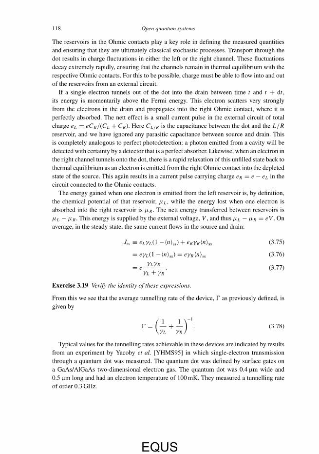
Lγ Rγ

DRAIN

SOURCE

µS Dµ VSDe=

c

µS

Dµ

L

R

Fig. 3.1 A schematic representation of a quantum dot in the conduction band. Position runs from leftto right and energy runs vertically. The quasibound state in the dot is labelled c. The grey regionslabelled L and R represent metallic electronic states filled up to the local Fermi level. The differencein the Fermi levels between left and right is determined by the source–drain bias voltage as eVSD .

A quantum dot is a three-dimensional confining potential for electrons or holes in asemiconductor, and can be fabricated in a number of ways [Tur95]. We will consider a verysimple model in which the dot has only a single bound state for one electron. This is not asartificial as it may sound. Although a single quantum dot in fact contains a very large numberof electrons, at low temperatures this system of electrons is close to the Fermi ground state.In a semiconductor dot the ground state is typically a filled valence band and an unoccupiedconduction band. In a metallic dot (or grain as it sometimes called) the ground state isthe conduction band filled up to the Fermi energy. At low temperatures and weak bias thecurrent is carried by a few electrons near the Fermi energy and we are typically concernedonly with additional electrons injected onto the dot. Because electrons are charged, largeenergy gaps can appear in the spectrum of multi-electron quantum dots, in addition to thequantization of energy levels due to confinement. This phenomenon is called Coulombblockade [Kas93]. The Coulomb blockade energy required to add a single electron to aquantum dot is e2/(2C), where the capacitance C can be very small (less than 10−16 F) dueto the small size of these systems. If the charging energy is large enough, compared withthermal energy, we can assume that only a single bound state for an additional electron isaccessible in the quantum dot. Typically this would require a temperature below 1 K.

We also assume that the dot is coupled via tunnel junctions to two fermionic reservoirs;see Fig. 3.1. A tunnel junction is a region in the material from which charge carriersclassically would be excluded by energy conservation. While propagating solutions of theSchrodinger equation cannot be found in such a region, exponentially decaying amplitudescan exist. We will assume that the region is not so extensive that all amplitudes decay tozero, but small enough for the coupling, due to the overlap of amplitudes inside and outsidethe region, to be small. In that case the coupling between propagating solutions on eitherside of the region can be treated perturbatively.

EQUS


We assume that the reservoirs remain in the normal (Ohmic) conducting state. The totalsystem is not in thermal equilibrium due to the bias voltage VSD across the dot. However,the two reservoirs are held very close to thermal equilibrium at temperature T , but atdifferent chemical potentials through contact to an external circuit via an Ohmic contact.We refer to the fermionic reservoir with the higher chemical potential as the source (alsocalled the emitter) and the one with the lower chemical potential as the drain (also calledthe collector). The difference in chemical potentials is given by µS − µD = eVSD . In thiscircumstance, charge may flow through the dot, and an external current will flow. Thenecessity to define a chemical potential is the first major difference between fermionicsystems and the bosonic environments of quantum optics.

A perturbative master-equation approach to this problem is valid only if the resistance ofthe tunnel junction, R, is large compared with the quantum of resistance RQ. The physicalmeaning of this condition is as follows. If for simplicity we denote the bias voltage of thejunction as V , then the average current through the junction is V/R, so the tunnelling rate is� = V/(eR). Thus the typical time between tunnelling events is �−1 = eR/V . Now, if thelifetime of the quasibound state is τ , then, by virtue of the time–energy uncertainty relationdiscussed in Section 3.3.1, there is an uncertainty in the energy level of order �/τ . If theexternal potential is to control the tunnelling then this energy uncertainty must remain lessthan eV . Thus the lifetime must be at least of order �/(eV ). If we demand that the lifetimebe much less than the time between tunnelling events, so that the events do not overlap intime, we thus require �/(eV )� eR/V . This gives the above relation between R and thequantum of resistance.

The total Hamiltonian of a system composed of the two Fermi reservoirs, connected bytwo tunnel barriers to a single Fermi bound state, is (with � = 1)

HQD+leads =∑k

εSk a†k ak + εcc

†c +∑p

εDp b†pbp

+∑k

(T Sk c

†ak + T Sk∗a†k c)+

∑p

(T Dp b

†pc + T D

p∗c†bp). (3.64)

Here ak(a†k ), c(c†) and bp(b†p) are the fermion annihilation (creation) operators of electrons

in the source (S) reservoir, in the central quantum dot and in the drain (D) reservoir,respectively. Because of the fermion anticommutation relations, the dot is described by justtwo states.

Exercise 3.17 Show from Eqs. (3.61) and (3.62) that the eigenvalues for the fermionnumber operator a†l al are 0 and 1, and that, if the eigenstates are |0〉 and |1〉, respectively,then a†l |0〉 = |1〉.

The first three terms in Eq. (3.64) comprise H0. The energy of the bound state withoutbias is ε0, which under bias becomes εc = ε0 − αeV , where α is a structure-dependentcoefficient. The single-particle energies in the source and drain are, respectively, εSk =k2/(2m) and εDp = p2/(2m)− eV . The energy reference is at the bottom of the conduction

EQUS


band of the source reservoir. Here, and below, we are assuming spin-polarized electrons sothat we do not have to sum over the spin degree of freedom.

The fourth and fifth terms in the Hamiltonian describe the coupling between the quasi-bound electrons in the dot and the electrons in the reservoir. The tunnelling coefficients T S

k

and T Dp depend upon the profile of the potential barrier between the dot and the reservoirs,

and upon the bias voltage. We will assume that at all times the two reservoirs remain intheir equlibrium states despite the tunnelling of electrons. This is a defining characteristicof a reservoir, and comes from assuming that the dynamics of the reservoirs are much fasterthan those of the quasibound quantum state in the dot.

In the interaction frame the Hamiltonian may be written as

V (t) =2∑

j=1

c†ϒj (t)eiεct + cϒ†j (t)e−iεct , (3.65)

where the reservoir operators are given by

ϒ1(t) =∑k

T Sk ake

−iεSk t , ϒ2(t) =∑p

T Dp bpe−iεDp t . (3.66)

We now obtain an equation of motion for the state matrix ρ of the bound state in the dotby following the standard method in Section 3.2. The only non-zero reservoir correlationfunctions we need to compute are

IjN (t) =∫ t

0dt1〈ϒ†

j (t)ϒj (t1)〉e−iεc(t−t1), (3.67)

IjA(t) =∫ t

0dt1〈ϒj (t1)ϒ†

j (t)〉e−iεc(t−t1). (3.68)

Here N and A stand for normal (annihilation operators after creation operators) andantinormal (vice versa) ordering of operators – see Section A.5. In order to illustrate theimportant differences between the fermionic case and the bosonic case discussed previously,we will now explicitly evaluate the first of these correlation functions, I1N (t).

Using the definition of the reservoir operators and the assumed thermal Fermi distributionof the electrons in the source, we find

I1N (t) =∑k

nSk |T Sk |2∫ t

0dt1 exp[i(εSk − εc)(t − t1)]. (3.69)

Since the reservoir is a large system, we can introduce a density of states ρ(ω) as usual andreplace the sum over k by an integral to obtain

I1N (t) =∫ ∞

0dω ρ(ω)nS(ω)|T S(ω)|2

∫ 0

−tdτ e−i(ω−εc)τ , (3.70)

where we have also changed the variable of time integration. The dominant term in thefrequency integration will come from frequencies near εc because the time integration is

EQUS


significant at that point. For fermionic reservoirs, the expression for the thermal occupationnumber is [Dat95]

nS(ω) = [1+ e(ω−ωf )/kBT ]−1, (3.71)

where ωf is the Fermi energy (recall that � = 1). We assume that the bias is such that thequasibound state of the dot is below the Fermi level in the source. This implies that nearω = εc, and at low temperatures, the average occupation of the reservoir state is very closeto unity [Dat95].

Now we make the Markov approximation to derive an autonomous master equation asin Section 3.2. On extending the limits of integration from −t to −∞ in Eq. (3.70) asexplained before, I1N may be approximated by the constant

I1N (t) ≈ πρ(εc)|TS(εc)|2 ≡ γL/2. (3.72)

This defines the effective rate γL of injection of electrons from the source (the left reservoirin Fig. 3.1) into the quasibound state of the dot. This rate will have a complicated dependenceon the bias voltage through both εc and the coupling coefficients |TS(ω)|, which can bedetermined by a self-consistent band calculation. We do not address this issue; we simplyseek the noise properties as a function of the rate constants.

By evaluating all the other correlation functions under similar assumptions, we find thatthe quantum master equation for the state matrix representing the dot state in the interactionframe is given by

dρ

dt= γL

2(2c†ρc − cc†ρ − ρcc†)+ γR

2(2cρc† − c†cρ − ρc†c), (3.73)

where γL and γR are constants determining the rate of injection of electrons from the sourceinto the dot and from the dot into the drain, respectively.

From this master equation it is easy to derive the following equation for the meanoccupation number〈n(t)〉 = Tr[c†cρ(t)]:

d〈n〉dt= γL(1−〈n〉)− γR〈n〉. (3.74)

Exercise 3.18 Show this, and show that the steady-state occupancy of the dot is 〈n〉ss =γL/(γL + γR).

The effect of Fermi statistics is evident in Eq. (3.74). If there is an electron on the dot,〈n〉 = 1, and the occupation of the dot can decrease only by emission of an electron intothe drain at rate γR .

It is at this point that we need to make contact with measurable quantities. In the caseof electron transport, the measurable quantities reduce to current I (t) and voltage V (t).The measurement results are a time series of currents and voltages, which exhibit both sys-tematic and stochastic components. Thus I (t) and V (t) are classical conditional stochasticprocesses, driven by the underlying quantum dynamics of the quasibound state on the dot.

EQUS


The reservoirs in the Ohmic contacts play a key role in defining the measured quantitiesand ensuring that they are ultimately classical stochastic processes. Transport through thedot results in charge fluctuations in either the left or the right channel. These fluctuationsdecay extremely rapidly, ensuring that the channels remain in thermal equilibrium with therespective Ohmic contacts. For this to be possible, charge must be able to flow into and outof the reservoirs from an external circuit.

If a single electron tunnels out of the dot into the drain between time t and t + dt ,its energy is momentarily above the Fermi energy. This electron scatters very stronglyfrom the electrons in the drain and propagates into the right Ohmic contact, where it isperfectly absorbed. The nett effect is a small current pulse in the external circuit of totalcharge eL = eCR/(CL + CR). Here CL/R is the capacitance between the dot and the L/Rreservoir, and we have ignored any parasitic capacitance between source and drain. Thisis completely analogous to perfect photodetection: a photon emitted from a cavity will bedetected with certainty by a detector that is a perfect absorber. Likewise, when an electron inthe right channel tunnels onto the dot, there is a rapid relaxation of this unfilled state back tothermal equilibrium as an electron is emitted from the right Ohmic contact into the depletedstate of the source. This again results in a current pulse carrying charge eR = e − eL in thecircuit connected to the Ohmic contacts.

The energy gained when one electron is emitted from the left reservoir is, by definition,the chemical potential of that reservoir, µL, while the energy lost when one electron isabsorbed into the right reservoir is µR . The nett energy transferred between reservoirs isµL − µR . This energy is supplied by the external voltage, V , and thus µL − µR = eV . Onaverage, in the steady state, the same current flows in the source and drain:

Jss ≡ eLγL(1−〈n〉ss)+ eRγR〈n〉ss (3.75)

= eγL(1−〈n〉ss) = eγR〈n〉ss (3.76)

= eγLγR

γL + γR. (3.77)

Exercise 3.19 Verify the identity of these expressions.

From this we see that the average tunnelling rate of the device, � as previously defined, isgiven by

� =(

1

γL+ 1

γR

)−1

. (3.78)

Typical values for the tunnelling rates achievable in these devices are indicated by resultsfrom an experiment by Yacoby et al. [YHMS95] in which single-electron transmissionthrough a quantum dot was measured. The quantum dot was defined by surface gates ona GaAs/AlGaAs two-dimensional electron gas. The quantum dot was 0.4 µm wide and0.5 µm long and had an electron temperature of 100 mK. They measured a tunnelling rateof order 0.3 GHz.

EQUS

3.6 The Lindblad form and positivity 119

Box 3.2 Quantum dynamical semigroups

Formally solving the master equation for the state matrix defines a map from the statematrix at time 0 to a state matrix at later times t by Nt: ρ(0)→ ρ(t) = Nt ρ(0) forall times t ≥ 0. This dynamical map must be completely positive (see Box 1.3). Moreformally, we require a quantum dynamical semigroup [AL87], which is a family ofcompletely positive maps Nt for t ≥ 0 such that

� NtNs = Nt+s� Tr[(Nt ρ)A] is a continuous function of t for any state matrix ρ and Hermitian operator A.

The family forms a semigroup rather than a group because there is not necessarily anyinverse. That is, Nt is not necessarily defined for t < 0.

These conditions formally capture the idea of Markovian dynamics of a quantumsystem. (Note that there is no implication that all open-system dynamics must beMarkovian.) From these conditions it can be shown that there exists a superoperator Lsuch that

dρ(t)

dt= Lρ(t), (3.79)

where L is called the generator of the map Nt . That is,

ρ(t) = Nt ρ(0) = eLt ρ(0). (3.80)

Moreover, this L must have the Lindblad form.

3.6 The Lindblad form and positivity

We have seen a number of examples in which the dynamics of an open quantum system canbe described by an automonous differential equation (a time-independent master equation)for the state matrix of the system. What is the most general form that such an equation cantake such that the solution is always a valid state matrix? This is a dynamical version of thequestion answered in Box 1.3 of Chapter 1, which was as follows: what are the physicallyallowed operations on a state matrix? In fact, the question can be formulated in a way thatgeneralizes the notion of operations to a quantum dynamical semigroup – see Box. 3.2

It was shown by Lindblad in 1976 [Lin76] that, for a Markovian master equation ρ =Lρ,the generator of the quantum dynamics must be of the form

Lρ = −i[H , ρ]+K∑k=1

D[Lk]ρ, (3.81)

for H Hermitian and {Lj } arbitrary operators. Here D is the superoperator defined earlierin Eq. (3.29). For mathematical rigour [Lin76], it is also required that

∑Kk=1 L

†kLk be a

bounded operator, but that is often not satisfied by the operators we use, so this requirementis usually ignored. This form is known as the Lindblad form, and the operators {Lk}

EQUS

gjmilburn

Highlight


are called Lindblad operators. The superoperator L is sometimes called the Liouvilliansuperoperator, by analogy with the operator which generates the evolution of a classicalprobability distribution on phase space, and the term Lindbladian is also used.

Each term in the sum in Eq. (3.81) can be regarded as an irreversible channel. It isimportant to note, however, that the decomposition of the generator into the Lindblad formis not unique. We can reduce the ambiguity by requiring that the operators 1, L1, L2, . . ., Lk

be linearly independent. We are still left with the possibility of redefining the Lindbladoperators by an arbitrary K ×K unitary matrix Tkl :

Lk →K∑l=1

TklLl . (3.82)

In addition, L is invariant under c-number shifts of the Lindblad operators, accompaniedby a new term in the Hamiltonian:

Lk → Lk + χk, H → H − i

2

K∑k=1

(χ∗k Lk − H.c.

). (3.83)

Exercise 3.20 Verify the invariance of the master equation under (3.82) and (3.83).

In the case of a single irreversible channel, it is relatively simple to evaluate the completelypositive map Nt = exp(Lt) formally as

Nt =∞∑m=0

N (m)t , (3.84)

where the operations N (m)(t) are defined by

N (m)t =

∫ t

0dtm

∫ tm

0dtm−1 · · ·

∫ t2

0dt1 S(t − tm)X

×S(tm − tm−1)X · · ·S(t2 − t1)XS(t1), (3.85)

with N (0)t = S(t). Here the superoperators S and X are defined by

S(τ ) = J[e−τ (iH+L†L/2)

], (3.86)

X = J [L], (3.87)

where the superoperator J is as defined in Eq. (1.80).

Exercise 3.21 Verify the above expression for Nt by calculating N0 and ρ (t), whereρ(t) = Nt ρ(0). Also verify that Nt is a completely positive map, as defined in Chapter 1.

As we will see in Chapter 4, Eq. (3.85) can be naturally interpreted in terms of a stochasticevolution consisting of periods of smooth evolution, described by S(τ ), interspersed withjumps, described by X .

Most of the examples of open quantum systems that we have considered above led, undervarious approximations, to a Markov master equation of the Lindblad form. However, as

EQUS

3.7 Decoherence and the pointer basis 121

the example of Brownian motion (Section 3.4.2) showed, this is not always the case. Itturns out that the time-dependent Brownian-motion master equation (3.58) does preservepositivity. It is only when making the approximations leading to the time-independent, butnon-Lindblad, equation (3.60) that one loses positivity. Care must be taken in using masterequations such as this, which are not of the Lindblad form, because there are necessarilyinitial states yielding time-evolved states that are non-positive (i.e. are not quantum states atall). Thus autonomous non-Lindblad master equations must be regarded as approximations,but, on the other hand, the fact that one has derived a Lindblad-form master equation doesnot mean that one has an exact solution. The approximations leading to the high-temperaturespin–boson master equation (3.56) may be no more valid than those leading to the high-temperature Brownian-motion master equation (3.60), for example. Whether or not a givenopen system is well approximated by Markovian dynamics can be determined only by adetailed study of the physics.

3.7 Decoherence and the pointer basis

3.7.1 Einselection

We are now in a position to state, and address, one of the key problems of quantummeasurement theory: what defines the measured observable? Recall the binary systemand binary apparatus introduced in Section 1.2.4. For an arbitrary initial system (S) state,and appropriate initial apparatus (A) state, the final combined state after the measurementinteraction is

|� ′〉 =1∑

x=0

sx |x〉|y := x〉, (3.88)

where |x〉 and |y〉 denote the system and apparatus in the measurement basis. A measurementof the apparatus in this basis will yield Y = x with probability |sx |2, that is, with exactlythe probability that a direct projective measurement of a physical quantity of the formC =∑x c(x)|x〉S〈x| on the system would have given. On the other hand, as discussed inSection 1.2.6, one could make a measurement of the apparatus in some other basis. Forexample, measurement in a complementary basis |p〉A yields no information about thesystem preparation at all.

In general one could read out the apparatus in the arbitrary orthonormal basis

|φ0〉 = α∗|0〉 + β∗|1〉, (3.89)

|φ1〉 = β|0〉 − α|1〉, (3.90)

where |α|2 + |β|2 = 1. The state after the interaction between the system and the apparatuscan now equally well be written as

|� ′〉 = d0|ψ0〉S ⊗ |φ0〉A + d1|ψ1〉S ⊗ |φ1〉A, (3.91)

EQUS

gjmilburn

Highlight


where d0|ψ0〉S = αs0|0〉 + βs1|1〉 and d1|ψ1〉S = β∗s0|0〉 − α∗s1|1〉. Note that |ψ0〉 and|ψ1〉 are not orthogonal if |φ0〉 and |φ1〉 are different from |0〉 and |1〉.Exercise 3.22 Show that this is true except for the special case in which |s0| = |s1|.

It is apparent from the above that there is only one basis (the measurement basis) inwhich one should measure the apparatus in order to make an effective measurement ofthe system observable C. Nevertheless, measuring in other bases is equally permitted bythe formalism, and yields different sorts of information. This does not seem to accordwith our intuition that a particular measurement apparatus is constructed, often at greateffort, to measure a particular system quantity. The flaw in the argument, however, is thatit is often not possible on physical grounds to read out the apparatus in an arbitrary basis.Instead, there is a preferred apparatus basis, which is determined by the nature of theapparatus and its environment. This has been called the pointer basis [Zur81]. For a well-constructed apparatus, the pointer basis will correspond to the measurement basis as definedabove.

The pointer basis of an apparatus is determined by how it is built, without reference toany intended measured system to which it may be coupled. One expects the measurementbasis of the apparatus, |0〉, |1〉, to correspond to two macroscopic classically distinguishablestates of a particular degree of freedom of the apparatus. This degree of freedom could, forexample, be the position of a pointer, whence the name ‘pointer basis’. An apparatus forwhich the pointer could be in a superposition of two distinct macroscopic states does notcorrespond to our intuitive idea of a pointer. Thus we expect that the apparatus can neverenter a superposition of two distinct pointer states as Eq. (3.89) would require.

This is a kind of selection rule, called einselection (environmentally induced selection)by Zurek [Zur82]. In essence it is justified by an apparatus–environment interaction thatvery rapidly couples the pointer states to orthogonal environment (E) states:

|y〉|z := 0〉 → |y〉|z := y〉E, (3.92)

where here |z〉 denotes an environment state. This is identical in form to the originalsystem–apparatus interaction. However, the crucial point is that now the total state is

|� ′′〉 =1∑

x=0

sx |x〉|y := x〉|z := x〉. (3.93)

If we consider using a different basis {|φ0〉, |φ1〉} for the apparatus, we find that it is notpossible to write the total state in the form of Eq. (3.93). That is,

|� ′′〉 �=1∑

x=0

dx |ψx〉S|φx〉A|θx〉E, (3.94)

for any coefficients dx and states for the system and environment.

Exercise 3.23 Show that this is true except for the special case in which |s0| = |s1|.

EQUS

3.7 Decoherence and the pointer basis 123

Note that einselection does not solve the quantum measurement problem in that it doesnot explain how just one of the elements of the superposition in Eq. (3.93) appears to becomereal, with probability |sx |2, while the others disappear. The solutions to that problem areoutside the scope of this book. What the approach of Zurek and co-workers achieves is toexplain why, for macroscopic objects like pointers, some states are preferred over others inthat they are (relatively) unaffected by decoherence. Moreover, they have argued plausiblythat these states have classical-like properties, such as being localized in phase space. Thesestates are not necessarily orthogonal states, as in the example above, but they are practicallyorthogonal if they correspond to distinct measurement outcomes [ZHP93].

3.7.2 A more realistic model

The above example is idealized in that we considered only two possible environment states.In reality the pointer may be described by continuous variables such as position. In this case,it is easy to see how physical interactions lead to an approximate process of einselection inthe position basis. Most interactions depend upon the position of an object, and the positionof a macroscopic object such as a pointer will almost instantaneously become correlatedwith many degrees of freedom in the environment, such as thermal photons, dust particlesand so on. This process of decoherence rapidly destroys any coherence between states ofmacroscopically different position, but these states of relatively well-defined position arethemselves little affected by the decoherence process (as expressed ideally in Eq. (3.92)).

Decoherence in this pointer basis can be reasonably modelled using the Brownian-motion master equation introduced in Section 3.4.2. In this situation, the dominant term inthe master equation is the last one (momentum diffusion), so we describe the evolution ofthe apparatus state by

ρ = −γ λ−2T [X, [X, ρ]]. (3.95)

Here we have used γ for γ∞, and λT is the thermal de Broglie wavelength, (2MkBT )−1/2. Itis called this because the thermal equilibrium state matrix for a free particle, in the positionbasis

ρ(x, x ′) = 〈x|ρ|x ′〉, (3.96)

has the form ρ(x, x ′) ∝ exp[−(x − x ′)2/(4λ2T)]. That is, the characteristic coherence length

of the quantum ‘waves’ representing the particle (first introduced by de Broglie) is λT. Inthis position basis the above master equation is easy to solve:

ρ(x, x ′; t) = exp[−γ t(x − x ′)2/λ2T]ρ(x, x ′; 0). (3.97)

Exercise 3.24 Show this. Note that this does not give the thermal equilibrium distributionin the long-time limit because the dissipation and free-evolution terms have been omitted.

Let the initial state for the pointer be a superposition of two states, macroscopically dif-ferent in position, corresponding to two different pointer readings. Let 2s be the separation

EQUS


of the states, and σ their width. For s � σ , the initial state matrix can be well approximatedby

ρ(x, x ′; 0) = (1/2)[ψ−(x)+ ψ+(x)][ψ∗−(x ′)+ ψ∗+(x ′)], (3.98)

where

ψ±(x) = (2πσ 2)−1/4 exp[−(x ∓ s)2/(2σ 2)

]. (3.99)

That is, ρ(x, x ′; 0) is a sum of four equally weighted bivariate Gaussians, centred in (x, x ′)-space at (−s,−s), (−s, s), (s,−s) and (s, s). But the effect of the decoherence (3.95)on these four peaks is markedly different. The off-diagonal ones will decay rapidly, on atime-scale

τdec = γ−1

(λT

2s

)2

. (3.100)

For s � λT, as will be the case in practice, this decoherence time is much smaller than thedissipation time,

τdiss = γ−1. (3.101)

The latter will also correspond to the time-scale on which the on-diagonal peaks in ρ(x, x ′)change shape under Eq. (3.97), provided that σ ∼ λT . This seems a reasonable assumption,since one would wish to prepare a well-localized apparatus (small σ ), but if σ � λT thenit would have a kinetic energy much greater than the thermal energy kBT and so woulddissipate energy at rate γ anyway.

The above analysis shows that, under reasonable approximations, the coherences (theoff-diagonal terms) in the state matrix decay much more rapidly than the on-diagonal termschange. Thus the superposition is transformed on a time-scale t , such that τdec � t � τdiss,into a mixture of pointer states:

ρ(x, x ′; t) ≈ (1/2)[ψ−(x)ψ∗−(x ′)+ ψ+(x)ψ∗+(x)]. (3.102)

Moreover, for macroscopic systems this time-scale is very short. For example, if s = 1 mm,T = 300 K, M = 1 g and γ = 0.01 s−1, one finds (upon restoring � where necessary)τdec ∼ 10−37 s, an extraordinarily short time. On such short time-scales, it could well beargued that the Brownian-motion master equation is not valid, and that a different treatmentshould be used (see for example Ref. [SHB03]). Nevertheless, this result can be taken asindicative of the fact that there is an enormous separation of time-scales between that onwhich the pointer is reduced to a mixture of classical states and the time-scale on whichthose classical states evolve.

3.8 Preferred ensembles

In the preceding section we argued that the interaction of a macroscopic apparatus withits environment preserves classical states and destroys superpositions of them. From thesimple model of apparatus–environment entanglement in Eq. (3.92), and from the solution

EQUS

gjmilburn

Highlight

3.8 Preferred ensembles 125

to the (cut-down) Brownian-motion master equation (3.97), it is seen that the state matrixbecomes diagonal in this pointer basis. Moreover, from Eq. (3.92), the environment carriesthe information about which pointer state the system is in. Any additional evolution ofthe apparatus (such as that necessary for it to measure the system of interest) could causetransitions between pointer states, but again this information would also be carried in theenvironment so that at all times an observer could know where the apparatus is pointing,so to speak.

It would be tempting to conclude from the above examples that all one need do to findout the pointer basis for a given apparatus is to find the basis which diagonalizes its stateonce it has reached equilibrium with its environment. However, this is not the case, for tworeasons. The first reason is that the states forming the diagonal basis are not necessarilystates that are relatively unaffected by the decoherence process. Rather, as mentioned above,the latter states will in general be non-orthogonal. In that case the preferred representationof the equilibrium state matrix

ρss =∑k

℘kπk (3.103)

will be in terms of an ensemble E ={℘k, πk} of pure states, with positive weights ℘k ,represented by non-orthogonal projectors: πj πk �= δjkπk . The second reason, which isgenerally ignored in the literature on decoherence and the pointer basis, is that the merefact that the state of a system becomes diagonal in some basis, through entanglement withits environment, does not mean that by observing the environment one can find the systemto be always in one of those diagonal states. Once again, it may be that one has to considernon-orthogonal ensembles, as in Eq. (3.103), in order to find a set of states that allows aclassical description of the system. By this we mean that the system can be always knownto be in one of those states, but to make transitions between them.

The second point above is arguably the more fundamental one for the idea that decoher-ence explains the emergence of classical behaviour. That is, the basic idea of einselectionis that there is a preferred ensemble for ρss for which an ignorance interpretation holds.With this interpretation of Eq. (3.103) one would claim that the system ‘really’ is in one ofthe pure states πk , but that one happens to be ignorant of which πk (i.e. which k) pertains.The weight ℘k would be interpreted as the probability that the system has state πk . Forthis to hold, it is necessary that in principle an experimenter could know which state πk thesystem is in at all times by performing continual measurements on the environment withwhich the system interacts. The pertinent index k would change stochastically such thatthe proportion of time for which the system has state πk is ℘k . This idea was first identifiedin Ref. [WV98]. The first point in the preceding paragraph then says that the states in thepreferred ensemble should also be robust in the face of decoherence. For example, if thedecoherence is described by a Lindbladian L then one could use the criterion adopted inRef. [WV98]. This is that the average fidelity

F (t) =∑k

℘k Tr[πk exp(Lt) πk] (3.104)

EQUS


should have a characteristic decay time that is as long as possible (and, for macroscopicsystems, one hopes that this is much longer than that of a randomly chosen ensemble).

In the remainder of this section we are concerned with elucidating when an ignoranceinterpretation of an ensemble representing ρss is possible. As well as being important inunderstanding the role of decoherence, it is also relevant to quantum control, as will bediscussed in Chapter 6. Let us restrict the discussion to Lindbladians having a uniquestationary state defined by

Lρss = 0. (3.105)

Also, let us consider only stationary ensembles for ρss. Clearly, once the system has reachedsteady state such a stationary ensemble will represent the system for all times t . Then, asclaimed above, it can be proven that for some ensembles (and, in particular, often forthe orthogonal ensemble) there is no way for an experimenter continually to measure theenvironment so as to find out which state the system is in. We say that such ensembles arenot physically realizable (PR). However, there are other stationary ensembles that are PR.

3.8.1 Quantum steering

To appreciate physical realizability of ensembles, it is first necessary to understand aphenomenon discovered by Schrodinger [Sch35a] and described by him as ‘steering’3 (wewill call it quantum steering). This phenomenon was rediscovered (and generalized) byHughston, Jozsa and Wootters [HJW93]. Consider a system with state matrix ρ that ismixed solely due to its entanglement with a second system, the environment. That is, thereis a pure state |�〉 in a larger Hilbert space of system plus environment such that

ρ = Trenv[|�〉〈�|] . (3.106)

This purification always exists, as discussed in Section A.2.2. Then, for any ensemble{(πk, ℘k)}k that represents ρ, it is possible to measure the environment such that the systemstate is collapsed into one of the pure states πk with probability ℘k . This is sometimesknown as the Schrodinger–HJW theorem.

Quantum steering gives rigorous meaning to the ignorance interpretation of any particularensemble. It says that there will be a way to perform a measurement on the environment,without disturbing the system state on average, to obtain exactly the information as to whichstate the system is ‘really’ in. Of course, the fact that one can do this for any ensemble meansthat no ensemble can be fundamentally preferred over any other one, as a representation ofρ at some particular time t . To say that an ensemble is PR, however, requires justifying theignorance interpretation at all times (after the system has reached steady state). We nowestablish the conditions for an ensemble to be PR.

3 Schrodinger introduced this as an evocative term for the Einstein–Podolsky–Rosen effect [EPR35] involving entangled states.For a completely general formulation of steering in quantum information terms, see Refs. [WJD07, JWD07].

EQUS


3.8.2 Conditions for physical realizability

According to quantum steering, it is always possible to realize a given ensemble at someparticular time t by measuring the environment. This may involve measuring parts ofthe environment that interacted with the system an arbitrarily long time ago, but thereis nothing physically impossible in doing this. Now consider the future evolution of aparticular system state πk following this measurement. At time t + τ , it will have evolvedto ρk(t + τ ) = exp(Lτ )πk . This is a mixed state because the system has now becomere-entangled with its environment.

The system state can be repurified by making another measurement on its environment.However, if the same ensemble is to remain as our representation of the system state thenthe pure system states obtained as a result of this measurement at time t + τ must becontained in the set {πj : j}. Because of quantum steering, this will be possible if and onlyif ρk(t + τ ) can be represented as a mixture of these states. That is, for all k there mustexist a probability distribution

{wjk(τ ) : j

}such that

exp(Lτ )πk =∑j

wjk(τ )πj . (3.107)

If wjk(τ ) exists then it is the probability that the measurement at time t + τ yields the stateπj .

Equation (3.107) is a necessary but not sufficient criterion for the ensemble {(πj , ℘j ) : j}to be PR. We also require that the weights be stationary. That is, for all j and all τ ,

℘j =∑k

℘kwjk(τ ). (3.108)

Multiplying both sides of Eq. (3.107) by ℘k , and summing over k, then using Eq. (3.108)and Eq. (3.103) gives eLτ ρss = ρss, as required from the definition of ρss.

One can analyse these conditions further to obtain simple criteria that can be appliedin many cases of interest [WV01]. In particular, we will return to them in Chapter 6.For the moment, it is sufficient to prove that there are some ensembles that are PR andsome that are not. This is what was called in Ref. [WV01] the preferred-ensemble fact(the ‘preferred’ ensembles are those that are physically realizable). Moreover, for somesystems the orthogonal ensemble is PR and for others it is not. The models we consider arechosen for their simplicity (they are two-level systems), and are not realistic models for thedecoherence of a macroscopic apparatus.

3.8.3 Examples

First we consider an example in which the orthogonal ensemble is PR: the high temperaturespin–boson model. In suitably scaled time units, the Lindbladian in Eq. (3.56) isL = D[σz].In this example, there is no unique stationary state, but all stationary states are of the form

ρss = ℘−|σz := −1〉〈σz := −1| + ℘+|σz := 1〉〈σz := 1|. (3.109)

EQUS


Exercise 3.25 Show this.

The orthogonal ensemble thus consists of the σz eigenstates with weights ℘±. To determinewhether this ensemble is PR, we must consider the evolution of its members under theLindbladian. It is trivial to show that L|σz := ±1〉〈σz := ±1| = 0 so that these states donot evolve at all. In other words, they are perfectly robust, withwjk(τ ) = δjk in Eq. (3.107).It is easy to see that Eq. (3.108) is also satisfied, so that the orthogonal ensemble is PR.

Next we consider an example in which the orthogonal ensemble is not PR: the driven,damped two-level atom. In the zero-detuning and zero-temperature limit, the Lindbladianis defined by

Lρ = −i�

2[σx, ρ]+ γD[σ−]ρ. (3.110)

The general solution of the corresponding Bloch equations is

x(t) = ue−(γ /2)t , (3.111)

y(t) = c+eλ+t + c−eλ−t + yss, (3.112)

z(t) = c+γ − 4i�

4�eλ+t + c−

γ + 4i�

4�eλ−t + zss, (3.113)

with eigenvalues defined by

λ± = −3

4γ ± i� (3.114)

and c± are constants given by

c± = 1

8i�

[∓4�(w − zss)± (γ ± 4i�)(v − yss)], (3.115)

where u, v and w are used to represent the initial conditions of x, y and z. A modified Rabifrequency has been introduced,

� =√�2 − (γ /4)2, (3.116)

which is real for � > γ/4 and imaginary for � < γ/4. The steady-state solutions arexss = 0, yss = 2�γ/(γ 2 + 2�2) and zss = −γ 2/(γ 2 + 2�2), as shown in Exercise 3.10.

Exercise 3.26 Derive the above solution, using standard techniques for linear differentialequations.

In the Bloch representation, the diagonal states ofρss are found by extending the stationaryBloch vector forwards and backwards to where it intersects the surface of the Bloch sphere.That is, the two pure diagonal states are u

v

w

±

= 0±2�∓γ

(4�2 + γ 2)−1/2

. (3.117)

EQUS


xy

z

1

0

00

1

1

Fig. 3.2 Dynamics of two states on the Bloch sphere according to the master equation (3.110), for� = 10γ , with points every 0.1γ −1. The initial states are those that diagonalize the stationary Blochsphere, which are close to y = ±1. The stationary state is the dot close to the centre of the Blochsphere.

Using these as initial conditions, it is easy to prove that, for general t , x(t)y(t)z(t)

±

�= w±+(t)

u

v

w

+

+ w±−(t)

u

v

w

−

(3.118)

for any weights w±+(t), w±−(t). That is, the diagonal states evolve into states that are notmixtures of the original diagonal states, so it is not possible for an observer to know at alltimes that the system is in a diagonal state. The orthogonal ensemble is not PR. This isillustrated in Fig. 3.2.

There are, however, non-orthogonal ensembles that are PR for this system. More-over, there is a PR ensemble with just two members, like the orthogonal ensemble. Thisis the ensemble {(π+, 1/2), (π−, 1/2)}, where this time the two states have the Blochvectors u

v

w

±

=±

√1− y2

ss − z2ss

yss

zss

. (3.119)

EQUS


Using these as initial conditions, we find

x(t)y(t)z(t)

±

=u±e−γ t/2

yss

zss

. (3.120)

Obviously this can be written as a positively weighted sum of the two initial Bloch vectors,and averaging over the two initial states will give a sum that remains equal to the stationaryBloch vector. That is, the two conditions (3.107) and (3.108) are satisfied, and this ensembleis PR.

Exercise 3.27 Prove the above by explicitly constucting the necessary weights w±+(t) andw±−(t).

These results are most easily appreciated in the�� γ limit. Then the stationary solutionis an almost maximally mixed state, displaced slightly from the centre of the Bloch spherealong the y axis. The diagonal states then are close to σy eigenstates, while the states in thePR ensemble are close to σx eigenstates. In this limit the master-equation evolution (3.110)is dominated by the Hamiltonian term, which causes the Bloch vector to rotate around theσx axis. Thus, the y eigenstates are rapidly rotated away from their original positions, sothis ensemble is neither robust nor PR, but the x eigenstates are not rotated at all, and simplydecay at rate γ /2 towards the steady state, along the line joining them. Thus this ensembleis PR. Moreover, it can be shown [WB00] that this is the most robust ensemble accordingto the fidelity measure Eq. (3.104), with a characteristic decay time (half-life) of 2 ln 2/γ .These features are shown in Fig. 3.3.

The existence of a PR ensemble in this second case (where the simple picture of adiagonal pointer basis fails) is not happenstance. For any master equation there are in factinfinitely many PR ensembles. Some of these will be robust, and thus could be consideredpointer bases, and some will not. A full understanding of how PR ensembles arise willbe reached in Chapter 4, where we consider the conditional dynamics of a continuouslyobserved open system.

3.9 Decoherence in a quantum optical system

3.9.1 Theoretical analysis

In recent years the effects of decoherence have been investigated experimentally, mostnotably in a quantum optical (microwave) cavity [BHD+96]. To appreciate this experiment,it is necessary to understand the effect of damping of the electromagnetic field in a cavity atzero temperature on a variety of initial states. This can be described by the interaction-framemaster equation, Eq. (3.38):

ρ = γD[a]ρ. (3.121)

EQUS

gjmilburn

Highlight

3.9 Decoherence in a quantum optical system 131

xy

z

1

0

00

1

1

Fig. 3.3 Dynamics of two states on the Bloch sphere according to the master equation (3.110), for� = 10γ , with points every 0.1γ −1. The initial states are the two non-orthogonal states π± definedin Eq. (3.119), which are close to x = ±1. The stationary state is the dot close to the centre of theBloch sphere.

If we use the solution given in Eq. (3.85) we find that the general solution can be writtenas a Kraus sum,

ρ(t) =∞∑m=0

Mm(t)ρ(0)M†m(t), (3.122)

where

Mm(t) = (1− e−γ t )m/2

√m!

e−γ ta†a/2am. (3.123)

We can regard this as an expansion of the state matrix in terms of the number of photonslost from the cavity in time t .

Exercise 3.28 Prove Eq. (3.122) by simplifying Eq. (3.85) using the property that[a†a, a†] = a†.

Equation (3.122) can be solved most easily in the number-state basis. However, it israther difficult to prepare a simple harmonic oscillator in a number eigenstate. We encountersimple harmonic oscillators regularly in classical physics; springs, pendula, cantilevers etc.What type of state describes the kinds of motional states in which such oscillators are

EQUS


typically found? We usually identify simple harmonic motion by observing oscillations. Inthe presence of friction oscillatory motion will decay. To observe a sustained oscillation,we need to provide a driving force to the oscillator. This combination of driving and frictionreaches a steady state of coherent oscillation. In classical physics the resulting motion willhave a definite energy, so one might expect that this would be a means of preparing a quantumoscillator in an energy eigenstate. However, a number state is actually time-independent, sothis cannot be so. Quantum mechanically, the state produced by this mechanism does nothave a definite energy. For weakly damped oscillators (as in quantum optics), it is actuallya coherent state, as shown in Exercise 3.13. For the reasons just described, the coherentstate is regarded as the most classical state of motion for a simple harmonic oscillator. It isoften referred to as a semiclassical state. Another reason why coherent states are consideredclassical-like is their robustness with respect to the decoherence caused by damping.

Exercise 3.29 From Eq. (3.122) show that, for a damped harmonic oscillator in theinteraction frame, a coherent state simply decays exponentially. That is, if |ψ(0)〉 = |α〉then |ψ(t)〉 = |αe−γ t/2〉.Hint: Consider the effect of Mm(t) on a coherent state, using the fact that a|α〉 = α|α〉 andalso using the number-state expansion for |α〉.

Suppose we somehow managed to prepare a cavity field in a superposition of two coherentstates,

|ψ(0)〉 = N (|α〉 + |β〉), (3.124)

where the normalization constant is N−1 = √2+ 2 Re〈α|β〉. If |α − β| � 1 then thiscorresponds to a superposition of macroscopically different fields. Such a superposition isoften called a Schrodinger-cat state, after the thought experiment invented by Schrodingerwhich involves a superposition of a live cat and a dead cat [Sch35b].

We now show that such a superposition is very fragile with respect to even a very smallamount of damping. Using the solution (3.122), the state will evolve to

ρ(t) ∝ |α(t)〉〈α(t)| + |β(t)〉〈β(t)|+C(α, β, t)|α(t)〉〈β(t)| + C∗(α, β, t)|β(t)〉〈α(t)|, (3.125)

where α(t) = αe−γ t/2, β(t) = βe−γ t/2 and

C(α, β, t) = exp

{−1

2

[|α(t)|2 + |β(t)|2 − 2α(t)β∗(t)]

(1− eγ t )

}. (3.126)

Exercise 3.30 Show this, by the same method as in Exercise 3.29.

The state (3.125) is a superposition of two damped coherent states with amplitudes α(t)and β(t) with a suppression of coherence between the states through the factor C(α, β, t).Suppose we now consider times much shorter than the inverse of the amplitude decay rate,γ t � 1. The coherence-suppression factor is then given by

C(α, β, t) ≈ exp(−|α − β|2γ t/2

). (3.127)

EQUS


C

α

De Dg

α g

S

R1 2RS´

g iφαe αe iφ+( )

+ e iφαe αe iφ( )

[[ 2/

Fig. 3.4 A schematic diagram of the experiment performed by the Haroche group to investigate thedecoherence of oscillator coherent states. The atom is prepared in an appropriate Rydberg state.The cavities R1 and R2 each apply a π/2 pulse. The interaction with the cavity field in C producessuperpositions of coherent states. The final ionization detectors determine the atomic state of theatom. Figure 2 adapted with permission from M. Brune et al., Phys. Rev. Lett. 77, 4887, (1996).Copyrighted by the American Physical Society.

We thus see that at the very beginning the coherence does not simply decay at the same rateas the amplitudes, but rather at a decay rate that depends quadratically on the differencebetween the amplitudes of the initial superposed states. This is qualitatively the sameas was seen for Brownian motion in Section 3.7.2. For macroscopically different states(|α − β| � 1) the decoherence is very rapid. Once the coherence between the two stateshas become very small we can regard the state as a statistical mixture of the two coherentstates with exponentially decaying coherent amplitudes. The quantum character of theinitial superposition is rapidly lost and for all practical purposes we may as well regard theinitial state as a classical statistical mixture of the two ‘pointer states’. For this reason it isvery hard to prepare an oscillator in a Schrodinger-cat state. However, the decoherence wehave described has been observed experimentally for |α − β| ∼ 1.

3.9.2 Experimental observation

The experimental demonstration of the fast decay of coherence for two superposed coherentstates was first performed by the Haroche group in Paris using the cavity QED system ofRydberg atoms in microwave cavities [BHD+96]. The experiment is based on Ramseyfringe interferometry (see Box 1.4). A schematic diagram of the experiment is shown inFig. 3.4.

A two-level atomic system with ground state |g〉 and excited state |e〉 interacts witha cavity field in C. This cavity field is well detuned from the atomic resonance. Theground and excited states of the atom correspond to Rydberg levels with principal quantumnumbers 50 and 51. Such highly excited states have very large dipole moments and can

EQUS


thus interact very strongly with the cavity field even though it is well detuned from thecavity resonance. The effect of the detuned interaction is to change the phase of the fieldin the cavity. However, the sign of the phase shift is opposite for each of the atomic states.Using second-order perturbation theory, an effective Hamiltonian for this interaction canbe derived:

HC = χa†aσz, (3.128)

where σz = |e〉〈e| − |g〉〈g|, and χ = |�|2/(2δ), where � is the single-photon Rabi fre-quency and δ = ωa − ωc is the atom–cavity detuning. Thus decreasing the detuningincreases χ (which is desirable), but the detuning cannot be decreased too much or thedescription in terms of this effective interaction Hamiltonian becomes invalid.

Assume to begin that the cavity fields R1 and R2 in Fig. 3.4 above are resonant withthe atomic transition. Say the cavity C is initially prepared in a weakly coherent state |α〉(in the experiment |α| = 3.1) and the atom in the state (|g〉 + |e〉)/√2, using a π/2 pulsein cavity R1. Then in time τ the atom–cavity system will evolve under the Hamiltonian(3.128) to

|ψ(τ )〉 = 1√2

(|g〉|αeiφ〉 + |e〉|αe−iφ〉) , (3.129)

where φ = χτ/2.

Exercise 3.31 Verify this.

The state in Eq. (3.129) is an entangled state between a two-level system and an oscillator.Tracing over the atom yields a field state that is an equal mixture of two coherent statesseparated in phase by 2φ.

To obtain a state that correlates the atomic energy levels with coherent superpositions ofcoherent states, the atom is subjected to another π/2 pulse in cavity R2. This creates thefinal state

|ψ〉out = 1√2

[|g〉(|αeiφ〉 + |αe−iφ〉)+ |e〉(|αeiφ〉 − |αe−iφ〉)]. (3.130)

If one now determines that the atom is in the state |g〉 at the final ionization detectors, theconditional state of the field is

|ψg〉out = N+(|αeiφ〉 + |αe−iφ〉), (3.131)

where N+ is a normalization constant. Likewise, if the atom is detected in the excited state,

|ψe〉out = N−(|αeiφ〉 − |αe−iφ〉). (3.132)

These conditional states are superpositions of coherent states.In the preceding discussion we ignored the cavity decay since this is small on the time-

scale of the interaction between a single atom and the cavity field. In order to see theeffect of decoherence, one can use the previous method to prepare the field in a coherentsuperposition of coherent states and then let it evolve for a time T so that there is a significantprobability that at least one photon is lost from the cavity. One then needs to probe the

EQUS


0.2

0.1

η

0.0

0 1 2

Fig. 3.5 A plot of the two-atom correlation η versus the delay time between successive atoms for twodifferent values of the conditional phase shift. Figure 5(b) adapted with permission from M. Brune etal., Phys. Rev. Lett. 77, 4887, (1996). Copyrighted by the American Physical Society.

decohered field state. It is impossible to measure directly the state of a microwave cavityfield at the quantum level because of the low energy of microwave photons comparedwith optical photons. Instead the Haroche team used a second atom as a probe for thefield state. They then measured the state of the second atom, obtaining the conditionalprobabilities p(e|g) and p(e|e) (where the conditioning label refers to the result of the firstatom measurement). Since the respective conditional field states after the first atom aredifferent, these probabilities should be different. The extent of the difference is given by

η = p(e|e)− p(e|g). (3.133)

From the result (3.125), after a time τ the two conditional states will have decohered to

ρgeout(τ ) ∝ (|ατ eiφ〉〈ατ eiφ| + |ατ e−iφ〉〈ατ e−iφ |)

± (C(τ )|ατ eiφ〉〈ατ e−iφ | + C(τ )∗|ατ e−iφ〉〈ατ eiφ|), (3.134)

where ατ < α due to decay in the coherent amplitude and |C(τ )| < 1 due to the decayin the coherences as before. In the limit C(τ )→ 0, these two states are indistinguishableand so η→ 0. Thus, by repeating a sequence of double-atom experiments, the relevantconditional probabilities may be sampled and a value of η as a function of the delay timecan be determined. (In the experiment, an extra averaging was performed to determineη, involving detuning the cavities R1 and R2 from atomic resonance ω0 by a varyingamount �.)

In Fig. 3.5 we reproduce the results of the experimental determination of η for twodifferent values of the conditional phase shift, φ, as a function of the delay time τ in units

EQUS


of cavity relaxation lifetime Tr = 1/γ . As expected, the correlation signal decays to zero.Furthermore, it decays to zero more rapidly for larger conditional phase shifts. That is to say,it decays to zero more rapidly when the superposed states are further apart in phase-space.The agreement with the theoretical result is very good.

3.10 Other examples of decoherence

3.10.1 Quantum electromechanical systems

We now consider a simple model of a measured system in which the apparatus undergoesdecoherence due to its environment. In the model the measured system is a two-level system(with basis states |0〉 and |1〉) while the apparatus is a simple harmonic oscillator, drivenon resonance by a classical force. The coupling between the two-level system and theoscillator is assumed to change the frequency of the oscillator. The effective Hamiltonianfor the system plus apparatus in the interaction frame is

H = ε(a† + a)+ χa†aσz, (3.135)

where ε is the strength of the resonant driving force and χ is the strength of the couplingbetween the oscillator and the two-level system. The irreversible dynamics of the apparatusis modelled using the weak-damping, zero-temperature master equation of Eq. (3.121),giving the master equation

ρ = −iε[a + a†, ρ]− iχ [a†aσz, ρ]+ γD[a]ρ. (3.136)

There are numerous physical problems that could be described by this model. It couldrepresent a two-level electric dipole system interacting with an electromagnetic cavity fieldthat is far detuned, as can occur in cavity QED (see the preceding Section 3.9.2) andcircuit QED (see the following Section 3.10.2). Another realization comes from the rapidlydeveloping field of quantum electromechanical systems, as we now discuss.

Current progress in the fabrication of nano-electromechanical systems (NEMSs) willsoon yield mechanical oscillators with resonance frequencies close to 1 GHz, and qualityfactors Q above 105 [SR05]. (The quality factor is defined as the ratio of the resonancefrequency ω0 to the damping rate γ .) At that scale, a NEMS oscillator becomes a quantumelectromechanical system (QEMS). One way to define the quantum limit is for the thermalexcitation energy to be less than the energy gap between adjacent oscillator energy eigen-states: �ω0 > kBT . This inequality would be satisfied by a factor of two or so with a devicehaving resonance frequency ω0 = 1× 2π GHz and temperature of T0 = 20 mK.

In this realization, the two-level system or qubit could be a solid-state double-wellstructure with a single electron tunnelling between the wells (quantum dots). We willmodel this as an approximate two-state system. It is possible to couple the quantum-electromechanical oscillator to the charge state of the double dot via an external voltagegate. A possible device is shown in Fig. 3.6. The two wells are at different distances from thevoltage gate and this distance is modulated as the oscillator moves. The electrostatic energy

EQUS

gjmilburn

Highlight

3.10 Other examples of decoherence 137

Q

1

2

L

Vg

DOUBLE QUANTUM DOT

1 2

d

Fig. 3.6 A possible scheme for coupling a single-electron double-dot system to a nano-mechanicalresonator. The double dot is idealized as a double-well potential for a single electron.

of the system depends on which well is occupied by the electron and on the square of theoscillator displacement. This leads to a shift in the frequency of the oscillator that dependson the location of the electron [CR98]. Currently such nano-mechanical electrometers arestrongly dominated by thermal fluctuations and the irreversible dynamics are not welldescribed by the decay term in Eq. (3.136). However, if quality factors and resonancefrequencies continue to increase, these devices should enter a domain of operation wherethis description is acceptable.

At any time the state of the system plus apparatus may be written as

ρ(t) = ρ00 ⊗ |0〉〈0| + ρ11 ⊗ |1〉〈1| + ρ10 ⊗ |1〉〈0| + ρ†10 ⊗ |0〉〈1|, (3.137)

where ρij is an operator that acts only in the oscillator Hilbert space. If we substitute thisinto Eq. (3.136), we find the following equations:

ρ 00 = −iε[a + a†, ρ00]+ iχ [a†a, ρ00]+ γD[a]ρ00, (3.138)

ρ 11 = −iε[a + a†, ρ11]− iχ [a†a, ρ11]+ γD[a]ρ11, (3.139)

ρ 10 = −iε[a + a†, ρ10]− iχ{a†a, ρ10} + γD[a]ρ10, (3.140)

where {A, B} = AB + BA as usual. On solving these equations for the initial condition ofan arbitary qubit state c0|0〉 + c1|1〉 and the oscillator in the ground state, we find that thecombined state of the system plus apparatus is

ρ(t) = |c0|2|α−(t)〉〈α−(t)| ⊗ |0〉〈0| + |c1|2|α+(t)〉〈α+(t)| ⊗ |1〉〈1|+ [c0c

∗1C(t)|α+(t)〉〈α−(t)| ⊗ |1〉〈0| + H.c.

], (3.141)

EQUS


where |α±(t)〉 are coherent states with amplitudes

α±(t) = −iε

γ /2± iχ

[1− ei−(γ /2±iχ )t

]. (3.142)

The coherence factorC(t) has a complicated time dependence, but tends to zero as t →∞.Thus the two orthogonal states of the measured qubit become classically correlated withdifferent coherent states of the apparatus. The latter are the pointer basis states of theapparatus, and may be approximately orthogonal. Even if they are not orthogonal, it can beseen that the qubit state becomes diagonal in the eigenbasis of σz.

For short times C(t) decays as an exponential of a quadratic function of time. Such aquadratic dependence is typical for coherence decay in a measurement model that reliesupon an initial build up of correlations between the measured system and the pointerdegree of freedom. For long times (γ t � 1), the coherence decays exponentially in time:C(t) ∼ e−�t . The rate of decoherence is

� = 2ε2γχ2

(γ 2/4+ χ2)2. (3.143)

This qubit decoherence rate can be understood as follows. The long-time solution ofEq. (3.141) is

ρ∞ = |c0|2|α−〉〈α−| ⊗ |0〉〈0| + |c1|2|α+〉〈α+| ⊗ |1〉〈1| (3.144)

with α± = −iε(γ /2± iχ )−1.

Exercise 3.32 Verify by direct substitution that this is a steady-state solution of the masterequation (3.136).

The square separation S = |α− − α+|2 between the two possible oscillator amplitudes inthe steady state is given by

S = 4ε2χ2

(γ 2/4+ χ2)2. (3.145)

Thus the long-time decoherence rate is � = Sγ/2. This is essentially the rate at whichinformation about which oscillator state is occupied (and hence which qubit state is occu-pied) is leaking into the oscillator’s environment through the damping at rate γ . If S � 1,then the decoherence rate is much faster than the rate at which the oscillator is damped.

3.10.2 A superconducting box

The international effort to develop a quantum computer in a solid-state system is drivinga great deal of fundamental research on the problem of decoherence. Recent experimentshave begun to probe the mechanisms of decoherence in single solid-state quantum devices,particularly superconducting devices. In this section we will consider the physical mecha-nisms of decoherence in these devices and recent experiments. A superconducting box orCooper-pair box (CPB) is essentially a small island of superconducting material separated

EQUS

3.10 Other examples of decoherence 139

TUNNELBARRIER

TUNNELBARRIER

xφ

Vg

Cg

ISLA

ND

Fig. 3.7 A Cooper-pair box system. A superconducting metallic island is connected to a Cooper pairreservoir by a split tunnel junction, threaded by a magnetic flux φx . A DC bias gate with voltage Vgcan make it energetically favourable for one or more Cooper-pairs to tunnel onto the island.

by a tunnel barrier from a reservoir of Cooper pairs. A Cooper pair (CP) is a pair of electronsbound together due to complex interactions with the lattice of the superconducting material[Coo56, BCS57]. Although electrons are fermions, a pair of electrons acts like a boson,and so can be described similarly to photons, using number states |N〉 for N ∈ N.

A schematic representation of a CPB is shown in Fig. 3.7. The box consists of a smallsuperconducting metallic island with oxide barrier tunnel junctions insulating it from theCooper-pair reservoir. As the voltage Vg on the bias gate is changed, one or more Cooperpairs may tunnel onto the island. The tunnelling rate is determined by the Josephson energyEJ of the junction. This can be changed by adjusting the magnetic flux φx threading theloop: a so-called split-junction CPB.

In the experiment of Schuster et al. [SWB+05] the CPB was placed inside a supercon-ducting co-planar microwave LC-resonator. The resonator supports a quantized mode ofthe electromagnetic field, while the CPB acts like an atomic system. Thus the term ‘circuitQED’ (as opposed to the ‘cavity QED’ of Section 3.9.2) is used for these systems. Thecoupling between the CPB and the microwave field is given by

H = �ωra†a − EJ

2

∑N

(|N〉〈N + 1| + |N + 1〉〈N |)+ 4EC

∑N

(N − ng)2|N〉〈N |. (3.146)

In the first term, ωr =√LC is the frequency and a the annihilation operator for the

microwave resonator field (note that in this section we are not setting � = 1). The secondterm is the Josephson tunnelling term, with Josephson frequency EJ/�. The third term isthe coupling between the field and the CPB, in whichEC = e2/(2C!) and ng = CgVg/(2e).HereC! is the capacitance between the island and the rest of the circuit,Cg is the capacitancebetween the CPB island and the bias gate for the island, and Vg is the operator for the totalvoltage applied to the island by the bias gate. This voltage can be split as Vg = V (0)

g + v,

EQUS


where V (0)g is a DC field and v is the microwave field in the cavity, which is quantized. It is

related to the cavity annihilation operator by

v = (a + a†)√

�ωr/(2C). (3.147)

We can thus write

ng = n(0)g + δng; δng(t) = [Cg/(2e)]v(t). (3.148)

For δng small, we can choose the bias n(0)g such that the CPB never has more than one

CP on it at any time. That is, we can restrict the Hilbert space to the N ∈ {0, 1} subspace,and write the Hamiltonian as

�ωra†a − 2EC(1− 2n(0)

g )σz − EJ

2σz − 4EC δng(t)(1− 2n(0)

g − σx). (3.149)

Here (differing from the usual convention) we have defined σx = |0〉〈0| − |1〉〈1| and σz =|1〉〈0| + |0〉〈1|. If one chooses to operate at the charge-degeneracy point, n(0)

g = 1/2, theHamiltonian takes the form

H = �ωra†a + �ωaσz/2− �g(a + a†)σx, (3.150)

where

g = eCg

C!

√ωr

�LC, ωa = EJ

�. (3.151)

Defining H0 = �ωa(a†a + σz/2), we move to an interaction frame with respect to thisHamiltonian, and make a rotating-wave approximation as usual. The new Hamiltonian is

V = ��a†a + �g(aσ+ + a†σ−), (3.152)

with � = ωr − ωa the detuning between the circuit frequency and the CPB tunnellingfrequency. It is assumed to be small compared with ωa . We can, however, still considera detuning that is large compared with g. Treating the second term in Eq. (3.152) as aperturbation on the first term, it is possible to show using second-order perturbation theorythat Eq. (3.152) may be approximated by the effective Hamiltonitan

Veff = ��a†a + �χa†aσz, (3.153)

where χ = g2/�. Moving frames again to the cavity resonance, and including a resonantmicrowave driving field ε, gives a Hamiltonian with the same form as Eq. (3.135).

Schuster et al. [SWB+05] recently implemented this system experimentally and mea-sured the measurement-induced qubit dephasing rate given in Eq. (3.143). In their exper-iment, �/(2π ) = 100 MHz, g/(2π ) = 5.8 MHz and the cavity decay rate was γ /(2π ) =0.8 MHz. Schoelkopf’s team used a second probe microwave field tuned to the CPB reso-nance to induce coherence in the qubit basis. The measurement-induced decoherence timethen appears as a broadening of the spectrum representing the response of the qubit tothe probe. This spectrum is related to the norm squared of the Fourier transform of thecoherence function in time. The results are found to be in good agreement with the theory

EQUS

3.11 Heisenberg-picture dynamics 141

presented here for small χ . Although the decay of coherence is exponential for long timeswith rate (3.143), for short times the decoherence is quadratic in time. This is manifestedexperimentally in the line shape of the probe absorption spectrum: the line shape deviatesfrom the usual Lorentzian shape (corresponding to exponential decay) in its wings.

3.11 Heisenberg-picture dynamics

We saw in Section 1.3.2 that quantum dynamics, and even quantum measurement, can beformulated in the Heisenberg picture. It is thus not surprising that there is a Heisenberg-picture formulation for master equations. This formulation is sometimes called the quantumstochastic differential-equation technique, or the quantum Langevin approach [GC85] (afterPaul Langevin, who developed the corresponding theory of classical stochastic differentialequations early in the twentieth century [Lan08]). In this section we will develop theHeisenberg-picture description for a system coupled to a bosonic (harmonic-oscillator)bath. We will show how the Markovian limit can be elegantly formulated in the Heisenbergpicture, and used to derive a Lindblad-form master equation.

Consider the interaction-frame coupling Hamiltonian in the rotating-wave approximation(3.24) derived in Section 3.3.1

VIF(t) = −i[b(z := −t)c† − b†(z := −t)c], (3.154)

where

b(z) = γ−1/2∑k

gkbke+iδkz, (3.155)

where δk is the detuning of the bath mode k from the system, γ is the dissipation rate, and,as in the example of Section 3.3.1, ic is the system lowering operator multiplied by

√γ .

We use z, rather than t , as the argument of b for two reasons. The first is that b(z := −t)is not at this stage a Heisenberg-picture operator. Rather, the interaction Hamiltonian istime-dependent because we are working in the interaction frame, and the operator b(z) isdefined simply to make VIF(t) simple in form. The second reason is that in some quantum-optical situations, such as the damping of a cavity mode at a single mirror, it is possibleto consider the electromagnetic field modes which constitute the bath as being functionsof one spatial direction only. On defining the speed of light in vacuo to be unity, and theorigin as the location of the mirror, we have that, at time t = 0, b(z) relates to the bath atposition |z| away from the mirror. For z < 0 it represents a property of the incoming field,and for z > 0 it represents a property of the outgoing field. That is, b(z := −t) representsthe field that will interact (for t > 0) or has interacted (for t < 0) with the system at timet . An explanation of this may be found in many textbooks, such as that of Gardiner andZoller [GZ04].

Now, in the limit of a continuum bath as considered in Section 3.3.1, we find that

[b(z), b†(z′)] = γ−1�(z− z′). (3.156)

EQUS


In order to derive a Markovian master equation, it was necessary to assume that �(τ ) wassharply peaked at τ = 0. Ignoring the Lamb shift in Eq. (3.30), and taking the Markovianlimit, we obtain

[b(z), b†(z′)] = δ(z− z′). (3.157)

Physically, this result cannot be exact because the bath modes all have positive frequency.Also, one must be careful using this result because of the singularity of the δ-function.Nevertheless, it is the result that must be used to obtain a strict correspondence with aMarkovian master equation.

Before moving to the Heisenberg picture, it is useful to define the unitary operator foran infinitesimal evolution generated by Eq. (3.154):

U (t + dt, t) = exp[cdB

†z:=−t − c†dBz:=−t

]. (3.158)

Here we have defined a new infinitesimal operator,

dBz = b(z)dt. (3.159)

The point of defining this infinitesimal is that, although it appears to be of order dt , becauseof the singularity of the commutation relation (3.157), it is actually of order

√dt . This can

be seen by calculating its commutation relations

[dBz, dB†z ] = dt, (3.160)

where we have used the heuristic equation δ(0)dt = 1. This can be understood by thinkingof dt as the smallest unit into which time can be divided. Then the discrete approximationto a δ-function is a function which is zero everywhere except for an interval of size dtaround zero, where it equals δ(0) = 1/dt (so that its area is unity). Because dBz is of order√

dt , it is necessary to expand U (t + dt, t) to second rather than first order in its argument.That is,

U (t + dt, t) = 1+(c dB†

z:=−t − c† dBz:=−t)− 1

2 c†c dt − 1

2 {c†, c}dB†z:=−t dBz:=−t

+ 12 c

2(

dB†z:=−t

)2+ 1

2 (c†)2(dBz:=−t

)2. (3.161)

Exercise 3.33 Show this, using Eq. (3.160).

3.11.1 Quantum Langevin equations

To obtain the Heisenberg-picture dynamics of the system, one might think that all one needdo is to write down the usual Heisenberg equations of motion (in the interaction frame)generated by the Hamiltonian (3.154). That is, for an arbitrary system operator s,

ds(t)

dt= [b(z := −t, t)c†(t)− b†(z := −t, t)c(t), s(t)], (3.162)

EQUS


where now b(z, t) is also time-dependent through the evolution of bk(t) in the Heisenbergpicture. However, because of the singularity of the commutation relation (3.157), thesituation is not so simple. The approach we will follow is different from that in most texts.It has the advantage of being simple to follow and of having a close relation to an analogousapproach in classical Markovian stochastic differential equations. For a detailed discussion,see Appendix B.

In our approach, to find the correct Heisenberg equations one proceeds as follows (notethat all unitaries are in the interaction frame as usual):

s(t + dt) = U †(t + dt, t0)s(t0)U (t + dt, t0) (3.163)

= U †(t, t0)U †(t + dt, t)s(t0)U (t + dt, t)U (t, t0) (3.164)

= U†HP(t + dt, t)s(t)UHP(t + dt, t), (3.165)

where s(t) = U †(t, t0)s(t0)U (t, t0) and

UHP(t + dt, t) ≡ U †(t, t0)U (t + dt, t)U (t, t0). (3.166)

Here we are (just for the moment) using the subscript HP to denote that Eq. (3.166) isobtained by replacing the operators appearing in U (t + dt, t) by their Heisenberg-pictureversions at time t . If we were to expand the exponential in UHP(t + dt, t) to first order in itsargument, we would simply reproduce Eq. (3.162). As motivated above, this will not work,and instead we must use the second-order expansion as in Eq. (3.161). First we define

dBin(t) ≡ dBz:=−t (t), (3.167)

and bin(t) similarly. These are known as input field operators. Note that as usual thet-argument on the right-hand side indicates that here dBz:=−t is in the Heisenberg picture.Because of the bath commutation relation (3.157), this operator is unaffected by anyevolution prior to time t , since dBin(t) commutes with dB†

in(t) for non-equal times. Thuswe could equally well have defined

dBin(t) ≡ dBz:=−t (t ′), ∀t ′ ≤ t. (3.168)

In particular, if t ′ = t0, the initial time for the problem, then dBin(t) is the same as theSchrodinger-picture operator dBz:=−t appearing in U (t + dt, t) of Eq. (3.158).

If the bath is initially in the vacuum state, this leads to a significant simplification, aswe will now explain. Ultimately we are interested in calculating the average of system (orbath) operators. In the Heisenberg picture, such an average is given by

〈s(t)〉 = Tr[s(t)ρS ⊗ ρB] = TrS[〈0|s(t)|0〉ρS], (3.169)

where |0〉 is the vacuum bath state and ρS is the initial system state. Since dBin(t)|0〉 = 0 forall t , any expression involving dBin(t) and dB†

in(t) that is in normal order (see Section A.5)will contribute nothing to the average. Thus it is permissible to drop all normally orderedterms in Eq. (3.161) that are of second order in dBin(t). That is to say, we can drop all

EQUS


second-order terms in dBin(t) in Eq. (3.161) because we have already used

dBin(t)dB†in(t) = [dBin(t), dB†

in(t)]+ dB†in(t)dBin(t) = dt (3.170)

to obtain the non-zero second-order term − 12 c

†c dt in Eq. (3.161).Although they do not contribute to 〈ds(t)〉, first-order terms in the input field operator

must be kept because they will in general contribute (via a non-normally ordered product)to the change in an operator product such as〈d(r s)〉. That is because, not surprisingly, onemust consider second-order corrections to the usual product rule:

d(r s) = (dr)s + r(ds)+ (dr)(ds). (3.171)

One thus obtains from Eq. (3.165) the following Heisenberg equation of motion in theinteraction frame:

ds = dt(c†sc − 1

2

{c†c, s

}+ i[H , s])− [dB†

in(t)c − c†dBin(t), s]. (3.172)

Here we have dropped the time arguments from all operators except the input bath operators.We have also included a system Hamiltonian H , as could arise from having a non-zeroVS , or a Lamb-shift term, as discussed in Section 3.3.1. Remember that we are still inthe interaction frame – H here is not the same as the H = H0 + V for the system plusenvironment with which we started the calculation.

We will refer to Eq. (3.172) as a quantum Langevin equation (QLE) for s. The operators may be a system operator or it may be a bath operator. Because bin(t) is the bath operatorbefore it interacts with the system, it is independent of the system operator s(t). Hence forsystem operators one can derive⟨

ds

dt

⟩= ⟨(c†sc − 1

2 c†cs − 1

2 sc†c)+ i[H , s]

⟩. (3.173)

Although the noise terms in (3.172) do not contribute to Eq. (3.173), they are necessary inorder for Eq. (3.172) to be a valid Heisenberg equation of motion. If they are omitted thenthe operator algebra of the system will not be preserved.

Exercise 3.34 Show this. For specificity, consider the case c = √γ a, where a is an annihi-lation operator, and show that, unless these terms are included, [a(t), a†(t)] will not remainequal to unity.

The master equation. Note that Eq. (3.173) is Markovian, depending only on the averageof system operators at the same time. Therefore, it should be derivable from a Markovianevolution equation for the system in the Schrodinger picture. That is to say, there shouldexist a master equation for the system state matrix such that

〈s(t)〉 = Tr[sρ(t)]. (3.174)

EQUS


Here, the placement of the time argument indicates the picture (Heisenberg or Schrodinger).By inspection of Eq. (3.173), the corresponding master equation is

ρ = D[c]ρ − i[H , ρ]. (3.175)

As promised, this is of the Lindblad form.

3.11.2 Generalization for a non-vacuum bath

The above derivation relied upon the assumption that the bath was initially in the vacuumstate |0〉. However, it turns out that there are other bath states for which it is possibleto derive a Markovian QLE and hence a Markovian master equation. This generalizationincludes a bath with thermal noise and a bath with so-called broad-band squeezing. Insteadof the equation dBin(t)dB†

in(t) = dt, with all other second-order products ignorable and allfirst-order terms being zero on average, we have in the general case

dB†in(t)dBin(t) = N dt, (3.176)

dBin(t)dB†in(t) = (N + 1)dt, (3.177)

dBin(t)dBin(t) = M dt, (3.178)⟨dBin(t)

⟩ = β dt, (3.179)

while Eq. (3.160) still holds. The parameter N is positive, while M and β are complex,with M constrained by

|M|2 ≤ N (N + 1). (3.180)

This type of input field is sometimes called a white-noise field, because the bath correlationsare δ-correlated in time. That is, they are flat (like the spectrum of white light) in frequencyspace. A thermal bath is well approximated by a white-noise bath with M = 0 and N ={exp[�ω0/(kBT )]− 1}−1, where ω0 is the frequency of the system’s free oscillation. Onlya pure squeezed (or vacuum) bath attains the equality in Eq. (3.180).

Using these rules in expanding the unitary operator in Eq. (3.165) gives the followinggeneral QLE for a white-noise bath:

ds = i dt[H , s]+ 1

2

{(N + 1)(2c†sc − sc†c − c†cs)+N (2csc† − scc† − cc†s)

+ M[c†, [c†, s]]+M∗[c, [c, s]]}dt − [dB†

in c − c† dBin, s].

(3.181)

Here we have dropped time arguments but are still (obviously) working in the Heisenbergpicture.

Exercise 3.35 Derive Eq. (3.181).

EQUS


The corresponding master equation is evidently

ρ = (N + 1)D[c]ρ +ND[c†]ρ + M

2[c†, [c†, ρ]]+ M∗

2[c, [c, ρ]]

− i[H + i(β∗c − βc†), ρ]. (3.182)

Note that the effect of the non-zero mean field (3.179) is simply to add a driving term to theexisting system Hamiltonian H . Although not obviously of the Lindblad form, Eq. (3.182)can be written in that form, with three irreversible terms, as long as Eq. (3.180) holds.

Exercise 3.36 Show this.Hint: Define N ′ such that |M|2 = N ′(N ′ + 1) and consider three Lindblad operatorsproportional to c, c† and [c(N ′ +M∗ + 1)− c†(N ′ +M)].

3.12 Further reading

There is a large and growing literature on describing the evolution of open quantum systems,both with and without the Markovian assumption. For a review, see the book by Breuer andPetruccione [BP02]. One of the interesting developments since that book was published isthe derivation [PV05] of a Markovian master equation for Brownian motion starting fromEinstein’s original concept of Brownian motion. That is, instead of considering a particlecoupled to a bath of harmonic oscillators, a massive particle is made to suffer collisionsby being immersed in a bath of less massive particles in thermal equilibrium. Building onthe work of Diosi [Dio93], Petruccione and Vacchini [PV05] have rigorously derived aLindblad-form master equation that involves diffusion in position as well as momentum.

As we have discussed, the Lindblad form is the only form of a Markovian masterequation that corresponds to a completely positive map for the state. The question of whichnon-Markovian master equations give rise to completely positive evolution has recentlybeen addressed by Andersson, Cresser and Hall [ACH07]. They consider time-local non-Markovian master equations; that is, master equations with time-dependent coefficientssuch as those we discussed in Section 3.4. For finite-dimensional systems, they show howthe state map for any time may be constructed from the master equation, and give a simpletest for complete positivity. Conversely, they show that any continuous time-dependent mapcan be turned into a master equation.

In this chapter we have discussed master equations for systems that can exchange exci-tations with both fermionic and bosonic baths. However, when presenting the Heisenberg-picture dynamics (quantum Langevin equations) we considered only the case of a bosonicbath. The reason is that there is an important technical issue due to the anticommutationrelations between the fermionic driving field and those system operators which can changethe number of fermions within the system. This problem has been addressed in a recentpaper by Gardiner [Gar04].

The decoherence ‘programme’ described briefly in Section 3.7 has been reviewedrecently by Zurek, one of its chief proponents [Zur03]. For an excellent discussion of

EQUS

3.12 Further reading 147

some of the conceptual issues surrounding decoherence and the quantum measurementproblem, see the recent review by Schlosshauer [Sch04]. For an extensive investigationof physically realizable ensembles and robustness for various open quantum systemssee Refs. [WV02a, WV02b, ABJW05]. Finally, we note that an improved version of theSchrodinger-cat decoherence experiment of Section 3.9.2 has been performed, also by theHaroche group. The new results [DDS+08] allow reconstruction of the whole quantumstate (specifically, its Wigner function – see Section A.5), showing the rapid vanishing ofits nonclassical features under damping.

EQUS

References

[AAS+02] M. A. Armen, J. K. Au, J. K. Stockton, A. C. Doherty, and H. Mabuchi,Adaptive homodyne measurement of optical phase, Phys. Rev. Lett. 89,133602, (2002).

[AB61] Y. Aharonov and D. Bohm, Time in the quantum theory and theuncertainty relation for time and energy, Phys. Rev. 122, 1649, (1961).

[ABC+01] G. Alber, Th. Beth, Ch. Charnes, A. Delgado, M. Grassl, andM. Mussinger, Stabilizing distinguishable qubits against spontaneousdecay by detected-jump correcting quantum codes, Phys. Rev. Lett. 86,4402, (2001).

[ABC+03] ———, Detected-jump-error-correcting quantum codes, quantum errordesigns, and quantum computation, Phys. Rev. A 68, 012316, (2003).

[ABJW05] D. J. Atkins, Z. Brady, K. Jacobs, and H. M. Wiseman, Classicalrobustness of quantum unravellings, Europhys. Lett. 69, 163,(2005).

[ACH07] E. Andersson, J. D. Cresser, and M. J. W. Hall, Finding the Krausdecomposition from a master equation and vice versa, J. Mod. Opt. 54,1695, (2007).

[AD01] F. Albertini and D. D’Alessandro, Notions of controllability for quantummechanical systems, Proceedings of the 40th IEEE Conference onDecision and Control, vol. 2, IEEE, New York (also available aseprint:quant-ph/0106128), p. 1589, 2001.

[ADL02] C. Ahn, A. C. Doherty, and A. J. Landahl, Continuous quantum errorcorrection via quantum feedback control, Phys. Rev. A 65, 042301,(2002).

[AK65] E. Arthurs and J. L. Kelly, On the simultaneous measurement of a pair ofconjugate observables, Bell. Syst. Tech. J. 44, 725, (1965).

[AL87] R. Alicki and K. Lendi, Quantum dynamical semigroups andapplications, Lecture Notes in Physics, vol. 717, Springer, Berlin, 1987.

[Alt02] C. Altafini, Controllability of quantum mechanical systems by root spacedecomposition of su(n), J. Math. Phys. 43, 2051, (2002).

[AMW88] P. Alsing, G. J. Milburn, and D. F. Walls, Quantum nondemolitionmeasurements in optical cavities, Phys. Rev. A 37, 2970, (1988).

[Ash70] A. Ashkin, Atomic-beam deflection by resonance-radiation pressure,Phys. Rev. Lett. 25, 1321, (1970).

[Ash90] R. B. Ash, Information theory, Dover, New York, 1990.

430

References 431

[AWJ04] C. Ahn, H. M. Wiseman, and K. Jacobs, Quantum error correction forcontinuously detected errors with any number of error channels per qubit,Phys. Rev. A 70, 024302, (2004).

[AWM03] C. Ahn, H. M. Wiseman, and G. J. Milburn, Quantum error correction forcontinuously detected errors, Phys. Rev. A 67, 052310, (2003).

[Bal98] L. E. Ballentine, Quantum mechanics: A modern development, WorldScientific, Singapore, 1998.

[Ban01] K. Banaszek, Fidelity balance in quantum operations, Phys. Rev. Lett. 86,1366, (2001).

[Bar90] A. Barchielli, Direct and heterodyne detection and other applications ofquantum stochastic calculus to quantum optics, Quantum Opt. 2, 423,(1990).

[Bar93] ———, Stochastic differential equations and a posteriori states inquantum mechanics, Int. J. Theor. Phys. 32, 2221, (1993).

[BB00] Ya. M. Blanter and M. Buttiker, Shot noise in mesoscopic conductors,Phys. Rep. 336, 1, (2000).

[BBC+93] C. H. Bennett, G. Brassard, C. Crepeau, R. Jozsa, A. Peres, and W. K.Wootters, Teleporting an unknown quantum state via dual classical andEinstein–Podolsky–Rosen channels, Phys. Rev. Lett. 70, 1895, (1993).

[BBL04] S. A. Babichev, B. Brezger, and A. I. Lvovsky, Remote preparation of asingle-mode photonic qubit by measuring field quadrature noise, Phys.Rev. Lett. 92, 047903, (2004).

[BC94] S. L. Braunstein and C. M. Caves, Statistical distance and the geometry ofquantum states, Phys. Rev. Lett. 72, 3439, (1994).

[BCM96] S. L. Braunstein, C. M. Caves, and G. J. Milburn, Generalized uncertaintyrelations: Theory, examples, and Lorentz invariance, Annals Phys. 247,135, (1996).

[BCS57] J. Bardeen, L. N. Cooper, and J. R. Schrieffer, Theory ofsuperconductivity, Phys. Rev. 108, 1175, (1957).

[BCS+04] M. D. Barrett, J. Chiaverini, T. Schaetz, J. Britton, W. M. Itano, J. D. Jost,E. Knill, C. Langer, D. Leibfried, R. Ozeri, and D. J. Wineland,Deterministic quantum teleportation of atomic qubits, Nature 429, 737,(2004).

[BDD05] J. Bylander, T. Duty, and P. Delsing, Current measurement by real-timecounting of single electrons, Nature 434, 361, (2005).

[Bel64] J. S. Bell, On the Einstein–Podolsy–Rosen paradox, Physics 1, 195,(1964), reprinted in Ref. [Bel87].

[Bel83] V. P. Belavkin, Towards the theory of the control of observable quantumsystems, Autom. Remote Control 44, 178, (1983) (also available aseprint:quant-ph/0408003).

[Bel87] J. S. Bell, Speakable and unspeakable in quantum mechanics, CambridgeUniversity Press, Cambridge, 1987.

[Bel88] V. P. Belavkin, Nondemolition measurement and nonlinear filtering ofquantum stochastic processes, Lecture Notes in Control and InformationSciences, Springer, Berlin, p. 245, 1988.

[Bel99] ———, Measurement, filtering and control in quantum open dynamicalsystems, Rep. Math. Phys. 43, 405, (1999).

[Bel02] ———, Quantum causality, stochastics, trajectories and information,Rep. Prog. Phys. 65, 353, (2002).

432 References

[Ber94] P. R. Berman (ed.), Cavity quantum electrodynamics (advances in atomic,molecular and optical physics), Academic Press, Boston, MA, 1994.

[BF28] M. Born and V. Fock, Beweis des Adiabatensatzes, Z. Phys. 51, 165–180,(1928).

[BFK00] S. L. Braunstein, C. A. Fuchs, and H. J. Kimble, Criteria forcontinuous-variable quantum teleportation, J. Mod. Opt. 47, 267,(2000).

[BFM02] T. A. Brun, J. Finkelstein, and N. D. Mermin, How much stateassignments can differ, Phys. Rev. A 65, 032315, (2002).

[BGS+99] B. C. Buchler, M. B. Gray, D. A. Shaddock, T. C. Ralph, and D. E.McClelland, Suppression of classical and quantum radiation pressurenoise via electro-optic feedback, Opt. Lett. 24, 259, (1999).

[BH93] D. Bohm and B. J. Hiley, The undivided universe: An ontologicalinterpretation of quantum theory, Routledge, London, 1993.

[BHD+96] M. Brune, E. Hagley, J. Dreyer, X. Maıtre, A. Maali, C. Wunderlich, J.-M.Raimond, and S. Haroche, Observing the progressive decoherence of the‘meter’ in a quantum measurement, Phys. Rev. Lett. 77, 4887, (1996).

[BHIW86] J. C. Bergquist, R. G. Hulet, W. M. Itano, and D. J. Wineland, Observationof quantum jumps in a single atom, Phys. Rev. Lett. 57, 1699, (1986).

[BK92] V. B. Braginsky and F. Y. Khalili, Quantum measurement, CambridgeUniversity Press, Cambridge, 1992.

[BK98] S. L. Braunstein and H. J. Kimble, Teleportation of continuous quantumvariables, Phys. Rev. Lett. 80, 869, (1998).

[BM03] S. D. Barrett and G. J. Milburn, Measuring the decoherence rate in asemiconductor charge qubit, Phys. Rev. B 68, 155307, (2003).

[BM04] A. J. Berglund and H. Mabuchi, Feedback controller design for tracking asingle fluorescent molecule, Appl. Phys. B. 78, 653, (2004).

[BMG+07] A. M. Branczyk, P. E. M. F. Mendonca, A. Gilchrist, A. C. Doherty, andS. D. Bartlett, Quantum control of a single qubit, Phys. Rev. A 75,012329, (2007).

[Boh13] N. Bohr, On the constitution of atoms and molecules, Phil. Mag. 26, 1,(1913).

[BP02] H.-P. Breuer and F. Petruccione, The theory of open quantum systems,Oxford University Press, Oxford, 2002.

[BR97] S. M. Barnett and E. Riis, Experimental demonstration of polarizationdiscrimination at the Helstrom bound, J. Mod. Opt. 44, 1061, (1997).

[BR05] D. E. Browne and T. Rudolph, Resource-efficient linear optical quantumcomputation, Phys. Rev. Lett. 95, 010501, (2005).

[Bro73] R. W. Brockett, Lie theory and control systems defined on spheres, SIAMJ. Appl. Math. 25, 213, (1973).

[BRS+05] T. M. Buehler, D. J. Reilly, R. P. Starrett, A. D. Greentree, A. R.Hamilton, A. S. Dzurak, and R. G. Clark, Single-shot readout with theradio-frequency single-electron transistor in the presence of charge noise,Appl. Phys. Lett. 86, 143117, (2005).

[BRW+06] P. Bushev, D. Rotter, A. Wilson, F. Dubin, C. Becher, J. Eschner, R. Blatt,V. Steixner, P. Rabl, and P. Zoller, Feedback cooling of a single trappedion, Phys. Rev. Lett. 96, 043003, (2006).

[BS92] V. P. Belavkin and P. Staszewski, Nondemolition observation of a freequantum particle, Phys. Rev. A 45, 1347, (1992).

References 433

[BS94] J. M. Bernardo and A. F. M. Smith, Bayesian theory, Wiley, Chichester,1994.

[BSSM07] L. Bouten, J. Stockton, G. Sarma, and H. Mabuchi, Scattering ofpolarized laser light by an atomic gas in free space: A quantumstochastic differential equation approach, Phys. Rev. A 75, 052111,(2007).

[BP86] S. M. Barnett and D. T. Pegg, Phase in quantum optics, J. Phys. A 19,3849, (1986).

[But88] M. Buttiker, Symmetry of electrical conduction, IBM J. Res. Dev. 32,317–334, (1988).

[BvH08] L. Bouten and R. van Handel, On the separation principle of quantumcontrol, Quantum Stochastics and Information: Statistics, Filtering andControl (V. P. Belavkin and M. I. Guta, eds.), World Scientific, Singapore,p. 206, 2008 (also available as eprint: math-ph/0511021).

[BW00] D. W. Berry and H. M. Wiseman, Optimal states and almost optimaladaptive measurements for quantum interferometry, Phys. Rev. Lett. 85,5098, (2000).

[BWB01] D. W. Berry, H. M. Wiseman, and J. K. Breslin, Optimal input states andfeedback for interferometric phase estimation, Phys. Rev. A 63, 053804,(2001).

[Car93] H. J. Carmichael, An open systems approach to quantum optics, Springer,Berlin, 1993.

[Car99] ———, Statistical methods in quantum optics, Vol. 1: Master equationsand Fokker–Planck equations, Springer, Berlin, 1999.

[Car07] ———, Statistical methods in quantum optics, Vol. 2: Non-classicalfields, Springer, Berlin, 2007.

[CBR91] H. J. Carmichael, R. J. Brecha, and P. R. Rice, Quantum interference andcollapse of the wavefunction in cavity QED, Opt. Commun. 82, 73,(1991).

[CCBFO00] H. J. Carmichael, H. M. Castro-Beltran, G. T. Foster, and L. A. Orozco,Giant violations of classical inequalities through conditional homodynedetection of the quadrature amplitudes of light, Phys. Rev. Lett. 85, 1855,(2000).

[CCBR01] R. B. M. Clarke, A. Chefles, S. M. Barnett, and E. Riis, Experimentaldemonstration of optimal unambiguous state discrimination, Phys. Rev. A63, 040305(R), (2001).

[CFS02a] C. M. Caves, C. A. Fuchs, and R. Schack, Conditions for compatibility ofquantum-state assignments, Phys. Rev. A 66, 062111, (2002).

[CFS02b] ———, Quantum probabilities as Bayesian probabilities, Phys. Rev. A65, 022305, (2002).

[Che00] A. Chefles, Quantum state discrimination, Contemp. Phys. 41, 401,(2000).

[CHP03] J. M. Courty, A. Heidmann, and M. Pinard, Back-action cancellation ininterferometers by quantum locking, Europhys. Lett. 63, 226, (2003).

[CK85] R. J. Cook and H. J. Kimble, Possibility of direct observation of quantumjumps, Phys. Rev. Lett. 54, 1023, (1985).

[CKT94] H. J. Carmichael, P. Kochan, and L. Tian, Coherent states and openquantum systems: A comment on the Stern–Gerlach experiment andSchrodinger’s cat, Proceedings of the International Symposium on

434 References

Coherent States: Past, Present, and Future (D. H. Feng, J. R. Klauder, andM. R. Strayer, eds.), World Scientific, Singapore, p. 75, 1994.

[CM87] C. M. Caves and G. J. Milburn, Quantum-mechanical model forcontinuous position measurements, Phys. Rev. A 36, 5543, (1987).

[CM91] S. L. Campbell and C. D. Meyer, Generalized inverses of lineartransformations, Dover Publications, New York, 1991.

[CMG07] R. L. Cook, P. J. Martin, and J. M. Geremia, Optical coherent statediscrimination using a closed-loop quantum measurement, Nature 446,774, (2007).

[Con90] J. B. Conway, A course in functional analysis, 2nd edn, Springer, NewYork, 1990.

[Coo56] L. N. Cooper, Bound electron pairs in a degenerate Fermi gas, Phys. Rev.104, 1189, (1956).

[CR98] A. N. Cleland and M. L. Roukes, Nanostructure-based mechanicalelectrometry, Nature 392, 160, (1998).

[CRG89] C. Cohen-Tannoudji, J. Dupont Roc, and G. Grynberg, Photons andatoms: Introduction to quantum electrodynamics, Wiley-Interscience,New York, 1989.

[CSVR89] H. J. Carmichael, S. Singh, R. Vyas, and P. R. Rice, Photoelectronwaiting times and atomic state reduction in resonance fluorescence, Phys.Rev. A 39, 1200, (1989).

[CT06] T. M. Cover and J. A. Thomas, Elements of information theory, 2nd edn,Wiley-Interscience, New York, 2006.

[CW76] H. J. Carmichael and D. F. Walls, Proposal for the measurement of theresonant Stark effect by photon correlation techniques, J. Phys. B 9, L43,(1976).

[CWJ08] J. Combes, H. M. Wiseman, and K. Jacobs, Rapid measurement ofquantum systems using feedback control, Phys. Rev. Lett. 100, 160503,(2008).

[CWZ84] M. J. Collett, D. F. Walls, and P. Zoller, Spectrum of squeezing inresonance fluorescence, Opt. Commun. 52, 145, (1984).

[D’A07] D. D’Alessandro, Introduction to quantum control and dynamics,Chapman & Hall, London, 2007.

[Dat95] S. Datta, Electronic transport in mesoscopic systems, CambridgeUniversity Press, Cambridge, 1995.

[Dav76] E. B. Davies, Quantum theory of open systems, Academic Press, London,1976.

[DCM92] J. Dalibard, Y. Castin, and K. Mølmer, Wave-function approach todissipative processes in quantum optics, Phys. Rev. Lett. 68, 580, (1992).

[DDS+08] S. Deleglise, I. Dotsenko, C. Sayrin, J. Bernu, M. Brune, J.-M. Raimond,and S. Haroche, Reconstruction of non-classical cavity field states withsnapshots of their decoherence, Nature 455, 510, (2008).

[DGKF89] J. C. Doyle, K. Glover, P. P. Khargonekar, and B. A. Francis, State-spacesolutions to standard H2 and H∞ control problems, IEEE Trans.Automatic Control 34, 831, (1989).

[DHJ+00] A. C. Doherty, S. Habib, K. Jacobs, H. Mabuchi, and S. M. Tan, Quantumfeedback control and classical control theory, Phys. Rev. A 62, 012105,(2000).

[Die88] D. Dieks, Overlap and distinguishability of quantum states, Phys. Lett. A126, 303–306, (1988).

References 435

[Dio88] L. Diosi, Localized solution of a simple nonlinear quantum Langevinequation, Phys. Lett. A 132, 233, (1988).

[Dio93] ———, On high-temperature Markovian equation for quantum Brownianmotion, Europhys. Lett. 22, 1, (1993).

[Dio08] ———, Non-Markovian continuous quantum measurement of retardedobservables, Phys. Rev. Lett. 100, 080401, (2008), Erratum ibid. 101,149902, (2008).

[Dir27] P. A. M. Dirac, The quantum theory of the emission and absorption ofradiation, Proc. Roy. Soc. London. A 114, 243, (1927).

[Dir30] ———, The principles of quantum mechanics, Clarendon Press, Oxford,1930.

[DJ99] A. C. Doherty and K. Jacobs, Feedback control of quantum systems usingcontinuous state estimation, Phys. Rev. A 60, 2700, (1999).

[DOG03] B. D’Urso, B. Odom, and G. Gabrielse, Feedback cooling of aone-electron oscillator, Phys. Rev. Lett. 90, 043001, (2003).

[Dol73] S. J. Dolinar, An optimum receiver for the binary coherent state quantumchannel, MIT Research Laboratory of Electronics Quarterly ProgressReport 111, 115, (1973).

[DPS02] A. C. Doherty, P. A. Parrilo, and F. M. Spedalieri, Distinguishingseparable and entangled states, Phys. Rev. Lett. 88, 187904, (2002).

[DPS03] G. M. D’Ariano, M. G. A. Paris, and M. F. Sacchi, Quantum tomography,Adv. Imaging Electron Phys. 128, 205, (2003).

[DZR92] R. Dum, P. Zoller, and H. Ritsch, Monte Carlo simulation of the atomicmaster equation for spontaneous emission, Phys. Rev. A 45, 4879, (1992).

[Ein17] A. Einstein, On the quantum theory of radiation, Phys. Z. 18, 121, (1917).[Eis05] J. Eisert, Optimizing linear optics quantum gates, Phys. Rev. Lett. 95,

040502, (2005).[EPR35] A. Einstein, B. Podolsky, and N. Rosen, Can quantum-mechanical

description of physical reality be considered complete?, Phys. Rev. 47,777, (1935).

[Fan57] U. Fano, Description of states in quantum mechanics by density matrixand operator techniques, Rev. Mod. Phys. 29, 74, (1957).

[FDF+02] J. D. Franson, M. M. Donegan, M. J. Fitch, B. C. Jacobs, and T. B.Pittman, High-fidelity quantum logic operations using linear opticalelements, Phys. Rev. Lett. 89, 137901, (2002).

[FF04] L. Fedichkin and A. Fedorov, Error rate of a charge qubit coupled to anacoustic phonon reservoir, Phys. Rev. A 69, 032311, (2004).

[FHWH07] C. Fricke, F. Hohls, W. Wegscheider, and R. J. Haug, Bimodal countingstatistics in single-electron tunneling through a quantum dot, Phys. Rev.B 76, 155307, (2007).

[FJ01] C. A. Fuchs and K. Jacobs, Information-tradeoff relations forfinite-strength quantum measurements, Phys. Rev. A 63, 062305, (2001).

[FMO00] G. T. Foster, S. L. Mielke, and L. A. Orozco, Intensity correlations incavity QED, Phys. Rev. A 61, 053821, (2000).

[FSB+98] A. Furusawa, J. L. Sørensen, S. L. Braunstein, C. A. Fuchs, H. J. Kimble,and E. S. Polzik, Unconditional quantum teleportation, Science 282, 706,(1998).

[FSRO02] G. T. Foster, W. P. Smith, J. E. Reiner, and L. A. Orozco, Time-dependentelectric field fluctuations at the subphoton level, Phys. Rev. A 66, 033807,(2002).

436 References

[Fuc96] C. A. Fuchs, Distinguishability and accessible information in quantumtheory, Ph.D. thesis, The University of New Mexico, Albuquerque, NM,1996 (also available as eprint:quant-ph/9601020).

[Gar85] C. W. Gardiner, Handbook of stochastic methods for physics, chemistryand the natural sciences, Springer, Berlin, 1985.

[Gar86] ———, Inhibition of atomic phase decays by squeezed light: A directeffect of squeezing, Phys. Rev. Lett. 56, 1917, (1986).

[Gar04] ———, Input and output in damped quantum systems III: Formulation ofdamped systems driven by fermion fields, Opt. Commun. 243, 57, (2004).

[GAW04] J. Gambetta, T. Askerud, and H. M. Wiseman, Jumplike unravelings fornon-Markovian open quantum systems, Phys. Rev. A 69, 052104, (2004).

[GBD+07] C. Guerlin, J. Bernu, S. Deleglise, C. Sayrin, S. Gleyzes, S. Kuhr,M. Brune, J.-M. Raimond, and S. Haroche, Progressive field-statecollapse and quantum non-demolition photon counting, Nature 448, 889,(2007).

[GBP97] M. Grassl, Th. Beth, and T. Pellizzari, Codes for the quantum erasurechannel, Phys. Rev. A 56, 33, (1997).

[GC85] C. W. Gardiner and M. J. Collett, Input and output in damped quantumsystems: Quantum stochastic differential equations and the masterequation, Phys. Rev. A 31, 3761, (1985).

[GC99] D. Gottesman and I. L. Chuang, Demonstrating the viability of universalquantum computation using teleportation and single-qubit operations,Nature 402, 390, (1999).

[GG01] F. Grosshans and P. Grangier, Quantum cloning and teleportation criteriafor continuous quantum variables, Phys. Rev. A 64, 010301, (2001).

[Gil83] D. T. Gillespie, A theorem for physicists in the theory of randomvariables, Am. J. Phys. 51, 520, (1983).

[Gil93] ———, Fluctuation and dissipation in Brownian motion, Am. J. Phys.61, 1077, (1993).

[Gil96] ———, The mathematics of Brownian motion and Johnson noise, Am. J.Phys. 64, 225, (1996).

[Gis89] N. Gisin, Stochastic quantum dynamics and relativity, Helv. Phys. Acta62, 363, (1989).

[GKG+07] S. Gleyzes, S. Kuhr, C. Guerlin, J. Bernu, S. Deleglise, U. B. Hoff,M. Brune, J.-M. Raimond, and S. Haroche, Quantum jumps of lightrecording the birth and death of a photon in a cavity, Nature 446, 297,(2007).

[Gla63] R. J. Glauber, The quantum theory of optical coherence, Phys. Rev. 130,2529, (1963).

[Gle57] A. M. Gleason, Measures on the closed subspaces of a Hilbert space,Indiana Univ. Math. J. 6, 885, (1957).

[GLM06] V. Giovannetti, S. Lloyd, and L. Maccone, Quantum metrology, Phys.Rev. Lett. 96, 010401, (2006).

[GM01] H-S. Goan and G. J. Milburn, Dynamics of a mesoscopic charge quantumbit under continuous quantum measurement, Phys. Rev. B 64, 235307,(2001).

[GMWS01] H-S. Goan, G. J. Milburn, H. M. Wiseman, and H.-B. Sun, Continuousquantum measurement of two coupled quantum dots using a point contact:A quantum trajectory approach, Phys. Rev. B 63, 125326, (2001).

References 437

[GN96] R. B. Griffiths and C-S. Niu, Semiclassical Fourier transform forquantum computation, Phys. Rev. Lett. 76, 3228, (1996).

[Goa03] H-S. Goan, An analysis of reading out the state of a charge quantum bit,Quantum Information Computation 3, 121, (2003).

[Got96] D. Gottesman, Class of quantum error-correcting codes saturating thequantum Hamming bound, Phys. Rev. A 54, 1862, (1996).

[GP92a] N. Gisin and I. C. Percival, The quantum-state diffusion model applied toopen systems, J. Phys. A 25, 5677, (1992).

[GP92b] ———, Wave-function approach to dissipative processes: Are therequantum jumps?, Phys. Lett. A 167, 315, (1992).

[GPS01] H. Goldstein, C. P. Poole, and J. L. Safko, Classical mechanics, 3rd edn,Addison-Wesley, Reading, MA, 2001.

[GPZ92] C. W. Gardiner, A. S. Parkins, and P. Zoller, Wave-function quantumstochastic differential equations and quantum-jump simulation methods,Phys. Rev. A 46, 4363, (1992).

[GSM04] J. M. Geremia, J. K. Stockton, and H. Mabuchi, Real-time quantumfeedback control of atomic spin-squeezing, Science 304, 270, (2004).

[GSM08] ———, Retraction, Science 321, 489a, (2008).[Gur97] S. A. Gurvitz, Measurements with a noninvasive detector and dephasing

mechanism, Phys. Rev. B 56, 15215, (1997).[GW01] J. Gambetta and H. M. Wiseman, State and dynamical parameter

estimation for open quantum systems, Phys. Rev. A 64, 042105, (2001).[GW02] ———, Non-Markovian stochastic Schrodinger equations:

Generalization to real-valued noise using quantum-measurement theory,Phys. Rev. A 66, 012108, (2002).

[GW03] ———, Interpretation of non-Markovian stochastic Schrodingerequations as a hidden-variable theory, Phys. Rev. A 68, 062104, (2003).

[GW04] ———, Modal dynamics for positive operator measures, FoundationsPhys. 34, 419, (2004).

[GWM93] M. J. Gagen, H. M. Wiseman, and G. J. Milburn, Continuous positionmeasurements and the quantum Zeno effect, Phys. Rev. A 48, 132,(1993).

[GZ04] C. W. Gardiner and P. Zoller, Quantum noise: A handbook of Markovianand non-Markovian quantum stochastic methods with applications toquantum optics, Springer, Berlin, 2004.

[Har02] L. Hardy, Why quantum theory?, Non-Locality and Modality (TomaszPlacek and Jeremy Butterfield, eds.), Nato Science Series: II, vol. 64,Kluwer, Dordrecht, p. 61, 2002.

[Haw71] A. G. Hawkes, Spectra of some self-exciting and mutually exciting pointprocesses, Biometrika 58, 83, (1971).

[HBB+07] B. L. Higgins, D. W. Berry, S. D. Bartlett, H. M. Wiseman, and G. J.Pryde, Entanglement-free Heisenberg-limited phase estimation, Nature450, 393, (2007).

[HDW+04] L. C. Hollenberg, A. S. Dzurak, C. Wellard, A. R. Hamilton, D. J. Reilly,G. J. Milburn, and R. G. Clark, Charge-based quantum computing usingsingle donors in semiconductors, Phys. Rev. B 69, 113301, (2004).

[Hei27] W. Heisenberg, Uber den anschaulichen Inhalt der quantentheoretischenKinematik und Mechanik, Z. Phys. 43, 172, (1927), English translation inRef. [WZ83].

438 References

[Hei30] ———, The physical principles of quantum mechanics, University ofChicago, Chicago, IL, 1930.

[Hel76] C. W. Helstrom, Quantum detection and estimation theory, Mathematicsin Science and Engineering, vol. 123, Academic Press, New York, 1976.

[HHM98] H. Hofmann, O. Hess, and G. Mahler, Quantum control by compensationof quantum fluctuations, Opt. Express 2, 339, (1998).

[HJHS03] A. Hopkins, K. Jacobs, S. Habib, and K. Schwab, Feedback cooling of ananomechanical resonator, Phys. Rev. B 68, 235328, (2003).

[HJW93] L. Hughston, R. Jozsa, and W. Wootters, A complete classification ofquantum ensembles having a given density matrix, Phys. Lett. A 183, 14,(1993).

[HK97] D. B. Horoshko and S. Ya. Kilin, Direct detection feedback for preservingquantum coherence in an open cavity, Phys. Rev. Lett. 78, 840, (1997).

[HMG+96] B. Huttner, A. Muller, J. D. Gautier, H. Zbinden, and N. Gisin,Unambiguous quantum measurement of nonorthogonal states, Phys. Rev.A 54, 3783, (1996).

[HMP+96] Z. Hradil, R. Myska, J. Perina, M. Zawisky, Y. Hasegawa, and H. Rauch,Quantum phase in interferometry, Phys. Rev. Lett. 76, 4295, (1996).

[Hol82] A. S. Holevo, Probabilistic and statistical aspects of quantum theory,Statistics and Probability, vol. 1, North-Holland, Amsterdam, 1982.

[Hol84] ———, Covariant measurements and imprimitivity systems, LectureNotes in Mathematics, vol. 1055, Springer, Berlin, p. 153, (1984).

[HOM87] C. K. Hong, Z. Y. Ou, and L. Mandel, Measurement of subpicosecondtime intervals between two photons by interference, Phys. Rev. Lett. 59,2044, (1987).

[HOW+05] L. Hollberg, C. W. Oates, G. Wilpers, C. W. Hoyt, Z. W. Barber, S. A.Diddams, W. H. Oskay, and J. C. Bergquist, Opticalfrequency/wavelength references, J. Phys. B 38, S469, (2005).

[HR85] F. Haake and R. Reibold, Strong damping and low-temperature anomaliesfor the harmonic oscillator, Phys. Rev. A 32, 2462, (1985).

[HTC83] G. M. Huang, T. J. Tarn, and J. W. Clark, On the controllability ofquantum-mechanical systems, J. Math. Phys. 24, 2608, (1983).

[Hus40] K. Husimi, Some formal properties of the density matrix, Proc. Phys.Math. Soc. Japan 22, 264, (1940).

[HWPC05] K. Hammerer, M. M. Wolf, E. S. Polzik, and J. I. Cirac, Quantumbenchmark for storage and transmission of coherent states, Phys. Rev.Lett. 94, 150503, (2005).

[HY86] H. A. Haus and Y. Yamamoto, Theory of feedback-generated squeezedstates, Phys. Rev. A 34, 270, (1986).

[Imr97] Y. Imry, Introduction to mesoscopic physics, Oxford University PressUSA, New York, 1997.

[Iva87] I. D. Ivanovic, How to differentiate between non-orthogonal states, Phys.Lett. A 123, 257, (1987).

[IW89] N. Ikeda and S. Watanabe, Stochastic differential equations and diffusionprocesses, 2nd edn, North-Holland, Amsterdam, 1989.

[Jac93] O. L. R. Jacobs, Introduction to control theory, Oxford University Press,Oxford, 1993.

[Jac03] K. Jacobs, How to project qubits faster using quantum feedback, Phys.Rev. A 67, 030301(R), (2003).

References 439

[Jac07] ———, Feedback control for communication with non-orthogonal states,Quantum Information Computation 7, 127, (2007).

[Jam04] M. R. James, Risk-sensitive optimal control of quantum systems, Phys.Rev. A 69, 032108, (2004).

[Jam05] ———, A quantum Langevin formulation of risk-sensitive optimalcontrol, J. Opt. B 7, S198, (2005).

[Jau68] J. M. Jauch, Foundations of quantum mechanics, Addison WesleyLongman, Reading, MA, 1968.

[JKP01] B. Julsgaard, A. Kozhekin, and E. S. Polzik, Experimental long-livedentanglement of two macroscopic objects, Nature 413, 400, (2001).

[JW85] E. Jakeman and J. G. Walker, Analysis of a method for the generation oflight with sub-Poissonian photon statistics, Opt. Commun. 55, 219,(1985).

[JWD07] S. J. Jones, H. M. Wiseman, and A. C. Doherty, Entanglement,Einstein–Podolsky–Rosen correlations, Bell nonlocality, and steering,Phys. Rev. A 76, 052116, (2007).

[Kas93] M. A. Kastner, Artificial atoms, Phys. Today 46, 24, (1993).[KDM77] H. J. Kimble, M. Dagenais, and L. Mandel, Photon antibunching in

resonance fluorescence, Phys. Rev. Lett. 39, 691, (1977).[KGB02] N. Khaneja, S. J. Glaser, and R. Brockett, Sub-Riemannian geometry and

time optimal control of three spin systems: Quantum gates and coherencetransfer, Phys. Rev. A 65, 032301, (2002).

[KJ93] S. Kotz and N. L. Johnson (eds.), Breakthroughs in statistics Vol. I,Springer, New York, 1993.

[KL97] E. Knill and R. Laflamme, Theory of quantum error-correcting codes,Phys. Rev. A 55, 900, (1997).

[KLM01] E. Knill, R. Laflamme, and G. J. Milburn, A scheme for efficient quantumcomputation with linear optics, Nature 409, 46, (2001).

[KLRG03] N. Khaneja, B. Luy, T. Reiss, and S. J. Glaser, Optimal control of spindynamics in the presence of relaxation, J. Magnetic Resonance 162, 311,(2003).

[KMN+07] P. Kok, W. J. Munro, K. Nemoto, T. C. Ralph, J. P. Dowling, and G. J.Milburn, Linear optical quantum computing with photonic qubits, Rev.Mod. Phys. 79, 135, (2007).

[Kor99] A. N. Korotkov, Continuous quantum measurement of a double dot, Phys.Rev. B 60, 5737, (1999).

[Kor01a] ———, Output spectrum of a detector measuring quantum oscillations,Phys. Rev. B 63, 085312, (2001).

[Kor01b] ———, Selective quantum evolution of a qubit state due to continuousmeasurement, Phys. Rev. B 63, 115403, (2001).

[Kor03] ———, Noisy quantum measurement of solid-state qubits: Bayesianapproach, Quantum Noise in Mesoscopic Physics (Y. V. Nazarov, ed.),Kluwer, Dordrecht, p. 205.

[Kor05] ———, Simple quantum feedback of a solid-state qubit, Phys. Rev. B 71,201305, (2005).

[KP00] P. E. Kloeden and E. Platen, Numerical solution of stochastic differentialequations, Springer, New York, 2000.

[Kra83] K. Kraus, States, effects, and operations: Fundamental notions ofquantum theory, Lecture Notes in Physics, vol. 190, Springer, Berlin,1983.

440 References

[KU93] M. Kitagawa and M. Ueda, Squeezed spin states, Phys. Rev. A 47, 5138,(1993).

[Lan08] P. Langevin, Sur la theorie du mouvement brownien, Comptes RendusAcad. Sci. (Paris) 146, 550, (1908), English translation by D. S. Lemonsand A. Gythiel, Am. J. Phys. 65, 1079, (1997).

[Lan88] R. Landauer, Spatial variation of currents and fields due to localizedscatterers in metallic conduction, IBM J. Res. Dev. 32, 306, (1988).

[Lan92] ———, Conductance from transmission: common sense points, Phys.Scripta T42, 110, (1992).

[LBCS04] M. D. LaHaye, O. Buu, B. Camarota, and K. C. Schwab, Approaching thequantum limit of a nanomechanical resonator, Science 304, 74, (2004).

[LCD+87] A. J. Leggett, S. Chakravarty, A. T. Dorsey, M. P. A. Fisher, A. Garg, andW. Zwerger, Dynamics of the dissipative two-state system, Rev. Mod.Phys. 59, 1, (1987).

[Lin76] G. Lindblad, On the generators of quantum dynamical semigroups,Commun. Math. Phys 48, 119, (1976).

[LJP+03] W. Lu, Z. Ji, L. Pfeiffer, K. W. West, and A. J. Rimberg, Real-timedetection of electron tunneling in a quantum dot, Nature 423, 422, (2003).

[Llo00] S. Lloyd, Coherent quantum feedback, Phys. Rev. A 62, 022108, (2000).[LM02] A. I. Lvovsky and J. Mlynek, Quantum-optical catalysis: Generating

nonclassical states of light by means of linear optics, Phys. Rev. Lett. 88,250401, (2002).

[LMPZ96] R. Laflamme, C. Miquel, J. P. Paz, and W. H. Zurek, Perfect quantumerror correcting code, Phys. Rev. Lett. 77, 198, (1996).

[LR91] P. Lancaster and L. Rodman, Solutions of continuous and discrete timealgebraic Riccati equations: A review, The Riccati Equation (S. Bittanti,A. J. Laub, and J. C. E. Willems, eds.), Springer, Berlin, p. 11, 1991.

[LR02] A. P. Lund and T. C. Ralph, Nondeterministic gates for photonicsingle-rail quantum logic, Phys. Rev. A 66, 032307, (2002).

[Lud51] G. Luders, Concerning the state-change due to the measurement process,Ann. Phys. (Leipzig) 8, 322, (1951), English translation by K. Kirkpatrickin Ann. Phys. (Leipzig), 15, 633, (2006).

[LWP+05] N. K. Langford, T. J. Weinhold, R. Prevedel, K. J. Resch, A. Gilchrist,J. L. O’Brien, G. J. Pryde, and A. G. White, Demonstration of a simpleentangling optical gate and its use in Bell-state analysis, Phys. Rev. Lett.95, 210504, (2005).

[LZG+07] C.-Y. Lu, X.-Q. Zhou, O. Guhne, W.-B. Gao, J. Zhang, Z.-S. Yuan,A. Goebel, T. Yang, and J.-W. Pan, Experimental entanglement of sixphotons in graph states, Nature Phys. 3, 91, (2007).

[Mab08] H. Mabuchi, Coherent-feedback quantum control with a dynamiccompensator, Phys. Rev. A 78, 032323, (2008).

[Maj98] F. G. Major, The quantum beat: The physical principles of atomic clocks,Lecture Notes in Physics, vol. 400, Springer, New York, 1998.

[MB99] G. J. Milburn and S. L. Braunstein, Quantum teleportation with squeezedvacuum states, Phys. Rev. A 60, 937, (1999).

[MCD93] K. Mølmer, Y. Castin, and J. Dalibard, Monte Carlo wave-functionmethod in quantum optics, J. Opt. Soc. Am. B 10, 524, (1993).

[MCSM] A. E. Miller, O. Crisafulli, A. Silberfarb, and H. Mabuchi, On thedetermination of the coherent spin-state uncertainty level, privatecommunication (2008).

References 441

[MD04] A. Migdall and J. Dowling, Special issue on single-photon: detectors,applications, and measurement methods (editorial), J. Mod. Opt. 51,1265, (2004).

[MdM90a] H. Martens and W. M. de Muynck, The inaccuracy principle, FoundationsPhys. 20, 357, (1990).

[MdM90b] H. Martens and W. M. de Muynck, Nonideal quantum measurements,Foundations Phys. 20, 255, (1990).

[Mer98] N. D. Mermin, What is QM trying to tell us?, Am. J. Phys. 66, 753, (1998).[MHF+90] J. Mertz, A. Heidmann, C. Fabre, E. Giacobino, and S. Reynaud,

Observation of high-intensity sub-Poissonian light using an opticalparametric oscillator, Phys. Rev. Lett. 64, 2897, (1990).

[MHF91] J. Mertz, A. Heidmann, and C. Fabre, Generation of sub-Poissonian lightusing active control with twin beams, Phys. Rev. A 44, 3229, (1991).

[Mil89] G. J. Milburn, Quantum optical Fredkin gate, Phys. Rev. Lett. 62, 2124,(1989).

[Mil93] P. Milonni, The quantum vacuum: An introduction to quantumelectrodynamics, Academic Press, Boston, MA, 1993.

[MK05] H. Mabuchi and N. Khaneja, Principles and applications of control inquantum systems, Int. J. Robust Nonlinear Control 15, 647–667,(2005).

[MMW05] S. Mancini, V. I. Man’ko, and H. M. Wiseman, Special issue on quantumcontrol (editorial), J. Opt. B 7, S177, (2005).

[Mol69] B. R. Mollow, Power spectrum of light scattered by two-level systems,Phys. Rev. 188, 1969, (1969).

[Møl97] K. Mølmer, Optical coherence: A convenient fiction, Phys. Rev. A 55,3195, (1997).

[MPV94] A. V. Masalov, A. A. Putilin, and M. V. Vasilyev, Sub-Poissonian lightand photocurrent shot-noise suppression in closed optoelectronic loop,J. Mod. Opt. 41, 1941, (1994).

[MY86] S. Machida and Y. Yamamoto, Observation of sub-Poissonianphotoelectron statistics in a negative feedback semiconductor laser, Opt.Commun. 57, 290, (1986).

[MZ96] H. Mabuchi and P. Zoller, Inversion of quantum jumps in quantum opticalsystems under continuous observation, Phys. Rev. Lett. 76, 3108,(1996).

[NC00] M. A. Nielsen and I. L. Chuang, Quantum computation and quantuminformation, Cambridge University Press, Cambridge, 2000.

[Nie01] M. A. Nielsen, Characterizing mixing and measurement in quantummechanics, Phys. Rev. A 63, 022114, (2001).

[Nie04] ———, Optical quantum computation using cluster states, Phys. Rev.Lett. 93, 040503, (2004).

[NM08] A. E. B. Nielsen and K. M Mølmer, Atomic spin squeezing in an opticalcavity, Phys. Rev. A 77, 063811, (2008).

[NRO+99] G. Nogues, A. Rauschenbeutel, S. Osnaghi, M. Brune, J.-M. Raimond,and S. Haroche, Seeing a single photon without destroying it, Nature 400,239, (1999).

[NSD86] W. Nagourney, J. Sandberg, and H. Dehmelt, Shelved optical electronamplifier: Observation of quantum jumps, Phys. Rev. Lett. 56, 2797,(1986).

442 References

[NWCL00] R. J. Nelson, Y. Weinstein, D. Cory, and S. Lloyd, Experimentaldemonstration of fully coherent quantum feedback, Phys. Rev. Lett. 85,3045, (2000).

[Nyq28] H. Nyquist, Thermal agitation of electric charge in conductors, Phys.Rev. 32, 110, (1928).

[OGW08] N. P. Oxtoby, J. Gambetta, and H. M. Wiseman, Model for monitoring ofa charge qubit using a radio-frequency quantum point contact includingexperimental imperfections, Phys. Rev. B 77, 125304, (2008).

[OPW+03] J. L. O’Brien, G. J. Pryde, A. G. White, T. C. Ralph, and D. Branning,Demonstration of an all-optical quantum controlled-NOT gate, Nature426, 264, (2003).

[OWW+05] N. P. Oxtoby, P. Warszawski, H. M. Wiseman, H.-B. Sun, and R. E. S.Polkinghorne, Quantum trajectories for the realistic measurement of asolid-state charge qubit, Phys. Rev. B 71, 165317, (2005).

[Oxt07] N. Oxtoby, Keeping it real: A quantum trajectory approach to realisticmeasurement of solid-state quantum systems, Ph.D. thesis, GriffithUniversity, Brisbane, 2007.

[Pau80] W. Pauli, General principles of quantum mechanics, Springer,Heidelberg, 1980.

[PB97] D. T. Pegg and S. M. Barnett, Tutorial review: Quantum optical phase,J. Mod. Opt. 44, 225, (1997).

[PDR88] A. P. Peirce, M. A. Dahleh, and H. Rabitz, Optimal control ofquantum-mechanical systems: Existence, numerical approximation, andapplications, Phys. Rev. A 37, 4950, (1988).

[Pea89] P. Pearle, Combining stochastic dynamical state-vector reduction withspontaneous localization, Phys. Rev. A 39, 2277, (1989).

[Per88] A. Peres, How to differentiate between non-orthogonal states, Phys. Lett.A 128, 19, (1988).

[Per95] ———, Quantum theory: Concepts and methods, Springer, Berlin, 1995.[PJM+04] J. R. Petta, A. C. Johnson, C. M. Marcus, M. P. Hanson, and A. C.

Gossard, Manipulation of a single charge in a double quantum dot, Phys.Rev. Lett. 93, 186802, (2004).

[PPB98] D. T. Pegg, L. S. Phillips, and S. M. Barnett, Optical state truncation byprojection synthesis, Phys. Rev. Lett. 81, 1604, (1998).

[PR04] M. Paris and J. Rehacek (eds.), Quantum state estimation, Lecture Notesin Physics vol. 649, Springer, Berlin, 2004.

[Pre97] J. Preskill, Lecture notes on quantum computation, Lecture notesproduced for the California Institute of Technology, 1997,http://www.theory.caltech.edu/people/preskill/ph229.

[Pre98] ———, Reliable quantum computers, Proc. Roy. Soc. London. A 454,385, (1998).

[PV05] F. Petruccione and B. Vacchini, Quantum description of Einstein’sBrownian motion, Phys. Rev. E 71, 046134, (2005).

[PVK97] M. B. Plenio, V. Vedral, and P. L. Knight, Quantum error correction in thepresence of spontaneous emission, Phys. Rev. A 55, 67, (1997).

[PZ01] J. P. Paz and W. H. Zurek, Environment induced superselection and thetransition from quantum to classical, Coherent Matter Waves, LesHouches Session LXXII (R. Kaiser, C. Westbrook, and F. David, eds.),EDP Sciences, Springer, Berlin, p. 533, 2001.

References 443

[RB01] R. Raussendorf and H. J. Briegel, A one-way quantum computer, Phys.Rev. Lett. 86, 5188, (2001).

[RBH01] J.-M. Raimond, M. Brune, and S. Haroche, Manipulating quantumentanglement with atoms and photons in a cavity, Rev. Mod. Phys. 73,565, (2001).

[RDM02] B. Rahn, A. C. Doherty, and H. Mabuchi, Exact performance ofconcatenated quantum codes, Phys. Rev. A 66, 032304, (2002).

[RdVRMK00] H. Rabitz, R. de Vivie-Riedle, M. Motzkus, and K. Kompa, Whither thefuture of controlling quantum phenomena?, Science 288, 824, (2000).

[Red57] A. G. Redfield, On the theory of relaxation processes, IBM J. Res. Dev. 1,19–31, (1957).

[RK02] R. Ruskov and A. N. Korotkov, Quantum feedback control of a solid-statequbit, Phys. Rev. B 66, 041401, (2002).

[RK03] ———, Spectrum of qubit oscillations from generalized Bloch equations,Phys. Rev. B 67, 075303, (2003).

[RL98] T. C. Ralph and P. K. Lam, Teleportation with bright squeezed light, Phys.Rev. Lett. 81, 5668, (1998).

[RLBW02] T. C. Ralph, N. K. Langford, T. B. Bell, and A. G. White, Linear opticalcontrolled-not gate in the coincidence basis, Phys. Rev. A 65, 062324,(2002).

[RLW05] T. C. Ralph, A. P. Lund, and H. M. Wiseman, Adaptive phasemeasurements in linear optical quantum computation, J. Opt. B 7, S245,(2005).

[RSD+95] V. Ramakrishna, M. V. Salapaka, M. Dahleh, H. Rabitz, and A. Peirce,Controllability of molecular systems, Phys. Rev. A 51, 960, (1995).

[RSO+04] J. E. Reiner, W. P. Smith, L. A. Orozco, H. M. Wiseman, and J. Gambetta,Quantum feedback in a weakly driven cavity QED system, Phys. Rev. A70, 023819, (2004).

[SAB+06] M. Steffen, M. Ansmann, R. C. Bialczak, N. Katz, E. Lucero,R. McDermott, M. Neeley, E. M. Weig, A. N. Cleland, and J. M. Martinis,Measurement of the entanglement of two superconducting qubits via statetomography, Science 313, 1423, (2006).

[SAJM04] M. Sarovar, C. Ahn, K. Jacobs, and G. J. Milburn, Practical scheme forerror control using feedback, Phys. Rev. A 69, 052324, (2004).

[Sar06] M. Sarovar, Quantum control and quantum information, Ph.D. thesis,University of Queensland, Brisbane, 2006.

[Sch30] E. Schrodinger, Zum Heisenbergschen Unscharfeprinzip, Sitzungsber.Preuβ. Akad. Wiss. Berlin (Math.-Phys.) 19, 296, (1930), Englishtranslation by A. Angelow, M.-C. Batoni, On Heisenberg’s uncertaintyrelation, Bulg. J. Phys. 26, 193, (1999); also available aseprint:quant-ph/9903100.

[Sch35a] ———, Discussion of probability relations between separated systems,Proc. Camb. Phil. Soc. 31, 553, (1935).

[Sch35b] ———, Die gegenwartige Situation in der Quantenmechanik,Naturwissenschaften 23, 807, (1935), English translation by J. D.Trimmer, The present situation in quantum mechanics, Proc. Am. Phil.Soc. 124, 323, (1980).

[Sch49] P. A. Schilpp (ed.), Albert Einstein: Philosopher-scientist, Library ofLiving Philosophers, Evanston, IL, 1949.

444 References

[Sch86] B. L. Schumaker, Quantum mechanical pure states with Gaussian wavefunctions, Phys. Rep. 135, 317, (1986).

[Sch95] B. Schumacher, Quantum coding, Phys. Rev. A 51, 2738, (1995).[Sch04] M. Schlosshauer, Decoherence, the measurement problem, and

interpretations of quantum mechanics, Rev. Mod. Phys. 76, 1267,(2004).

[SD81] M. D. Srinivas and E. B. Davies, Photon counting probabilities inquantum optics, J. Mod. Opt. 28, 981, (1981).

[SDCZ01] A. Sørensen, L.-M. Duan, I. Cirac, and P. Zoller, Many-particleentanglement with Bose–Einstein condensates, Nature 409, 63, (2001).

[SDG99] W. T. Strunz, L. Diosi, and N. Gisin, Open system dynamics withnon-Markovian quantum trajectories, Phys. Rev. Lett. 82, 1801, (1999).

[SG64] L. Susskind and J. Glogower, Quantum mechanical phase and timeoperator, Physics 1, 49, (1964).

[Sha49] C. E. Shannon, Communication theory of secrecy systems, Bell Syst.Tech. J. 28, 656–715, (1949).

[SHB03] W. T. Strunz, F. Haake, and D. Braun, Universality of decoherence formacroscopic quantum superpositions, Phys. Rev. A 67, 022101,(2003).

[SJG+07] E. V. Sukhorukov, A. N. Jordan, S. Gustavsson, R. Leturcq, T. Ihn, andK. Ensslin, Conditional statistics of electron transport in interactingnanoscale conductors, Nature Phys. 3, 243, (2007).

[SJM+04] D. A. Steck, K. Jacobs, H. Mabuchi, T. Bhattacharya, and S. Habib,Quantum feedback control of atomic motion in an optical cavity, Phys.Rev. Lett. 92, 223004, (2004).

[SM95] B. C. Sanders and G. J. Milburn, Optimal quantum measurements forphase estimation, Phys. Rev. Lett. 75, 2944, (1995).

[SM01] A. J. Scott and G. J. Milburn, Quantum nonlinear dynamics ofcontinuously measured systems, Phys. Rev. A 63, 042101, (2001).

[SM05] M. Sarovar and G. J. Milburn, Continuous quantum error correction bycooling, Phys. Rev. A 72, 012306, (2005).

[SR05] K. C. Schwab and M. L. Roukes, Putting mechanics into quantummechanics, Phys. Today 58, 36, (2005).

[SRO+02] W. P. Smith, J. E. Reiner, L. A. Orozco, S. Kuhr, and H. M. Wiseman,Capture and release of a conditional state of a cavity QED system byquantum feedback, Phys. Rev. Lett. 89, 133601, (2002).

[SRZ05] V. Steixner, P. Rabl, and P. Zoller, Quantum feedback cooling of a singletrapped ion in front of a mirror, Phys. Rev. A 72, 043826, (2005).

[SS98] A. Shnirman and G. Schon, Quantum measurements performed with asingle-electron transistor, Phys. Rev. B 57, 15400, (1998).

[SSH+87] J. H. Shapiro, G. Saplakoglu, S. T. Ho, P. Kumar, B. E. A. Saleh, andM. C. Teich, Theory of light detection in the presence of feedback, J. Opt.Soc. Am. B 4, 1604, (1987).

[SSW90] J. J. Stefano, A. R. Subberud, and I. J. Williams, Theory and problems offeedback and control systems, 2nd edn, McGraw-Hill, New York, 1990.

[Ste96] A. M. Steane, Multiple-particle interference and quantum errorcorrection, Proc. Roy. Soc. London A 452, 2551, (1996).

[Ste07] ———, How to build a 300 bit, 1 giga-operation quantum computer,Quantum Information Computation 7, 171, (2007).

References 445

[Sto06] J. K. Stockton, Continuous quantum measurement of cold alkali-atomspins, Ph.D. thesis, California Institute of Technology, Pasadena, CA,2006.

[SV06] L. F. Santos and L. Viola, Enhanced convergence and robust performanceof randomized dynamical decoupling, Phys. Rev. Lett. 97, 150501, (2006).

[SvHM04] J. K. Stockton, R. van Handel, and H. Mabuchi, Deterministic Dicke-statepreparation with continuous measurement and control, Phys. Rev. A 70,022106, (2004).

[SW49] C. E. Shannon and W. Weaver, The mathematical theory ofcommunication, University of Illinois Press, Urbana, IL, 1949.

[SW07] R. W. Spekkens and H. M. Wiseman, Pooling quantum states obtained byindirect measurements, Phys. Rev. A 75, 042104, (2007).

[SWB+05] D. I. Schuster, A. Wallraff, A. Blais, L. Frunzio, R.-S. Huang, J. Majer,S. M. Girvin, and R. J. Schoelkopf, AC Stark shift and dephasing of asuperconducting qubit strongly coupled to a cavity field, Phys. Rev. Lett.94, 123602, (2005).

[SWK+98] R. J. Schoelkopf, P. Wahlgren, A. A. Kozhevnikov, P. Delsing, and D. E.Prober, The radio-frequency single-electron transistor (RF-SET): A fastand ultrasensitive electrometer, Science 280, 1238, (1998).

[TC68] M. Tavis and F. W. Cummings, Exact solution for an N-moleculeradiation-field Hamiltonian, Phys. Rev. 170, 379, (1968).

[TMB+06] A. M. Tyryshkin, J. J. L. Morton, S. C. Benjamin, A. Ardavan, G. A. D.Briggs, J. W. Ager, and S. A. Lyon, Coherence of spin qubits in silicon, J.Phys. C 18, S783, (2006).

[TMW02a] L. K. Thomsen, S. Mancini, and H. M. Wiseman, Continuous quantumnondemolition feedback and unconditional atomic spin squeezing, J.Phys. B 35, 4937, (2002).

[TMW02b] ———, Spin squeezing via quantum feedback, Phys. Rev. A 65, 061801,(2002).

[TRS88] P. R. Tapster, J. G. Rarity, and J. S. Satchell, Use of parametricdown-conversion to generate sub-Poissonian light, Phys. Rev. A 37, 2963,(1988).

[Tur95] R. Turton, The quantum dot: A journey into the future of microelectronics,W. H. Freeman, Oxford, 1995.

[TV08] F. Ticozzi and L. Viola, Quantum Markovian subsystems: Invariance,attractivity, and control, IEEE Trans. Automatic Control 53, 2048, (2008).

[TW02] L. K. Thomsen and H. M. Wiseman, Atom–laser coherence and itscontrol via feedback, Phys. Rev. A 65, 063607, (2002).

[TWMB95] M. S. Taubman, H. Wiseman, D. E. McClelland, and H.-A. Bachor,Intensity feedback effects on quantum-limited noise, J. Opt. Soc. Am. B12, 1792, (1995).

[Vai94] L. Vaidman, Teleportation of quantum states, Phys. Rev. A 49, 1473,(1994).

[VB96] L. Vandenberghe and S. Boyd, Semidefinite programming, Soc. Indust.Appl. Math. Rev. 38, 49, (1996).

[VES+04] L. M. K. Vandersypen, J. M. Elzerman, R. N. Schouten, L. H. Willemsvan Beveren, R. Hanson, and L. P. Kouwenhoven, Real-time detection ofsingle-electron tunneling using a quantum point contact, Appl. Phys. Lett.85, 4394, (2004).

446 References

[VL98] L. Viola and S. Lloyd, Dynamical suppression of decoherence intwo-state quantum systems, Phys. Rev. A 58, 2733, (1998).

[VLK99] L. Viola, S. Lloyd, and E. Knill, Universal control of decoupled quantumsystems, Phys. Rev. Lett. 83, 4888, (1999).

[vHM05] R. van Handel and H. Mabuchi, Optimal error tracking via quantumcoding and continuous syndrome measurement, arXive-print:quant-ph/0511221, 2005.

[vN32] J. von Neumann, Mathematische Grundlagen der Quantenmechanik,Springer, Berlin, 1932, English translation by E. T. Beyer, asMathematical Foundations of Quantum Mechanics (Princeton UniversityPress, Princeton, NJ, 1955).

[Wan01] X. Wang, Spin squeezing in nonlinear spin-coherent states, J. Opt. B 3,93, (2001).

[WB00] H. M. Wiseman and Z. Brady, Robust unravelings for resonancefluorescence, Phys. Rev. A 62, 023805, (2000).

[WB08] H. M. Wiseman and L. Bouten, Optimality of feedback control strategiesfor qubit purification, Quantum Information Processing 7, 71, (2008).

[WBI+92] D. J. Wineland, J. J. Bollinger, W. M. Itano, F. L. Moore, and D. J.Heinzen, Spin squeezing and reduced quantum noise in spectroscopy,Phys. Rev. A 46, R6797, (1992).

[WD01] H. M. Wiseman and L. Diosi, Complete parametrization, and invariance,of diffusive quantum trajectories for Markovian open systems, Chem.Phys. 268, 91, (2001), Erratum ibid. 271, 227 (2001).

[WD05] H. M. Wiseman and A. C. Doherty, Optimal unravellings for feedbackcontrol in linear quantum systems, Phys. Rev. Lett. 94, 070405, (2005).

[WG08] H. M. Wiseman and J. M. Gambetta, Pure-state quantum trajectories forgeneral non-Markovian systems do not exist, Phys. Rev. Lett. 101,140401, (2008).

[Whi81] P. Whittle, Risk-sensitive linear/quadratic/Gaussian control, Adv. Appl.Probability 13, 764, (1981).

[Whi96] ———, Optimal control: Basics and beyond, Wiley, Chichester, 1996.[Wig32] E. Wigner, On the quantum correction for thermodynamic equilibrium,

Phys. Rev. 40, 749, (1932).[Wis94] H. M. Wiseman, Quantum theory of continuous feedback, Phys. Rev. A

49, 2133, (1994), Errata ibid., 49 5159 (1994) and ibid. 50, 4428(1994).

[Wis95] ———, Adaptive phase measurements of optical modes: Going beyondthe marginal q distribution, Phys. Rev. Lett. 75, 4587, (1995).

[Wis98] ———, In-loop squeezing is like real squeezing to an in-loop atom, Phys.Rev. Lett. 81, 3840, (1998).

[Wis04] ———, Squeezing and feedback, Quantum Squeezing (P. D. Drummondand Z. Ficek, eds.), Springer, Berlin, p. 171, 2004.

[Wis06] ———, From Einstein’s theorem to Bell’s theorem: A history of quantumnon-locality, Contemp. Phys. 47, 79–88, (2006).

[Wis07] ———, Grounding Bohmian mechanics in weak values and Bayesianism,New J. Phys. 9, 165, (2007).

[WJ85a] J. G. Walker and E. Jakeman, Optical dead time effects andsub-Poissonian photo-electron counting statistics, Proc. Soc. Photo-Opt.Instrum. Eng. 492, 274, (1985).

References 447

[WJ85b] ———, Photon-antibunching by use of a photoelectron-event-triggeredoptical shutter, Opt. Acta 32, 1303, (1985).

[WJD07] H. M. Wiseman, S. J. Jones, and A. C. Doherty, Steering, entanglement,nonlocality, and the Einstein–Podolsky–Rosen paradox, Phys. Rev. Lett.98, 140402, (2007).

[WK97] H. M. Wiseman and R. B. Killip, Adaptive single-shot phasemeasurements: A semiclassical approach, Phys. Rev. A 56, 944, (1997).

[WK98] ———, Adaptive single-shot phase measurements: The full quantumtheory, Phys. Rev. A 57, 2169, (1998).

[WM93a] H. M. Wiseman and G. J. Milburn, Interpretation of quantum jump anddiffusion processes illustrated on the Bloch sphere, Phys. Rev. A 47,1652, (1993).

[WM93b] ———, Quantum theory of field-quadrature measurements, Phys. Rev. A47, 642, (1993).

[WM93c] ———, Quantum theory of optical feedback via homodyne detection,Phys. Rev. Lett. 70, 548, (1993).

[WM94a] D. F. Walls and G. J. Milburn, Quantum optics, Springer, Berlin, 1994.[WM94b] H. M. Wiseman and G. J. Milburn, All-optical versus electro-optical

quantum-limited feedback, Phys. Rev. A 49, 4110, (1994).[WM94c] ———, Squeezing via feedback, Phys. Rev. A 49, 1350, (1994).

[WMW02] H. M. Wiseman, S. Mancini, and J. Wang, Bayesian feedback versusMarkovian feedback in a two-level atom, Phys. Rev. A 66, 013807,(2002).

[Won64] W. M. Wonham, Some applications of stochastic differential equations tooptimal nonlinear filtering, J. Soc. Indust. Appl. Math., A 2, 347,(1964).

[Woo81] W. K. Wootters, Statistical distance and Hilbert space, Phys. Rev. D 23,357, (1981).

[WPW99] C. E. Wieman, D. E. Pritchard, and D. J. Wineland, Atom cooling,trapping, and quantum manipulation, Rev. Mod. Phys. 71, S253, (1999).

[WR06] H. M. Wiseman and J. F. Ralph, Reconsidering rapid qubit purification byfeedback, New J. Phys. 8, 90, (2006).

[WT99] H. M. Wiseman and G. E. Toombes, Quantum jumps in a two-level atom:Simple theories versus quantum trajectories, Phys. Rev. A 60, 2474,(1999).

[WT01] H. M. Wiseman and L. K. Thomsen, Reducing the linewidth of an atomlaser by feedback, Phys. Rev. Lett. 86, 1143, (2001).

[WUS+01] H. M. Wiseman, D. W. Utami, H.-B. Sun, G. J. Milburn, B. E. Kane,A. Dzurak, and R. G. Clark, Quantum measurement of coherent tunnelingbetween quantum dots, Phys. Rev. B 63, 235308, (2001).

[WV98] H. M. Wiseman and J. A. Vaccaro, Maximally robust unravelings ofquantum master equations, Phys. Lett. A 250, 241, (28 December 1998).

[WV01] ———, Inequivalence of pure state ensembles for open quantum systems:The preferred ensembles are those that are physically realizable, Phys.Rev. Lett. 87, 240402, (2001).

[WV02a] ———, Atom lasers, coherent states, and coherence. I. Physicallyrealizable ensembles of pure states, Phys. Rev. A 65, 043605, (2002).

[WV02b] ———, Atom lasers, coherent states, and coherence II. Maximally robustensembles of pure states, Phys. Rev. A 65, 043606, (2002).

448 References

[WW30] V. F. Weisskopf and E. P. Wigner, Berechnung der naturlichenLinienbreite auf Grund der Diracschen Lichttheorie, Z. Phys. 63, 54,(1930).

[WW01] J. Wang and H. M. Wiseman, Feedback-stabilization of an arbitrary purestate of a two-level atom, Phys. Rev. A 64, 063810, (2001).

[WW03a] P. Warszawski and H. M. Wiseman, Quantum trajectories for realisticphotodetection: I. General formalism, J. Opt. B 5, 1, (2003).

[WW03b] ———, Quantum trajectories for realistic photodetection: II. Applicationand analysis, J. Opt. B 5, 15, (2003).

[WWM01] J. Wang, H. M. Wiseman, and G. J. Milburn, Non-Markovianhomodyne-mediated feedback on a two-level atom: a quantum trajectorytreatment, Chem. Phys. 268, 221, (2001).

[WZ65] E. Wong and M. Zakai, On the relationship between ordinary andstochastic differential equations, Int. J. Eng. Sci. 3, 213, (1965).

[WZ83] J. A. Wheeler and W. H. Zurek, Quantum theory and measurement,Princeton University Press, Princeton, NJ, 1983.

[Yam06] N. Yamamoto, Robust observer for uncertain linear quantum systems,Phys. Rev. A 74, 032107, (2006).

[YHMS95] A. Yacoby, M. Heiblum, D. Mahalu, and H. Shtrikman, Coherence andphase sensitive measurements in a quantum dot, Phys. Rev. Lett. 74,4047, (1995).

[YIM86] Y. Yamamoto, N. Imoto, and S. Machida, Amplitude squeezing in asemiconductor laser using quantum nondemolition measurement andnegative feedback, Phys. Rev. A 33, 3243, (1986).

[YMK86] B. Yurke, S. L. McCall, and J. R. Klauder, SU(2) and SU(1,1)interferometers, Phys. Rev. A 33, 4033, (1986).

[ZDG96] K. Zhou, J. C. Doyle, and K. Glover, Robust and optimal control,Prentice-Hall, Upper Saddle River, NJ, 1996.

[ZHP93] W. H. Zurek, S. Habib, and J. P. Paz, Coherent states via decoherence,Phys. Rev. Lett. 70, 1187, (1993).

[ZRK05] Q. Zhang, R. Ruskov, and A. N. Korotkov, Continuous quantum feedbackof coherent oscillations in a solid-state qubit, Phys. Rev. B 72, 245322,(2005).

[Zur81] W. H. Zurek, Pointer basis of quantum apparatus: Into what mixture doesthe wave packet collapse?, Phys. Rev. D 24, 1516, (1981).

[Zur82] ———, Environment-induced superselection rules, Phys. Rev. D 26,1862, (1982).

[Zur03] ———, Decoherence, einselection, and the quantum origins of theclassical, Rev. Mod. Phys. 75, 715, (2003).

[ZVTR03] S. Zippilli, D. Vitali, P. Tombesi, and J.-M. Raimond, Scheme fordecoherence control in microwave cavities, Phys. Rev. A 67, 052101,(2003).

quantum measurement and control - arc centre of excellence for

Documents