Quantum Maxwell-Bloch equationsfor spatially inhomogeneous semiconductor lasers

Holger F. Hofmann and Ortwin HessTheoretical Quantum Electronics,Institute of Technical Physics, DLR

Pfaffenwaldring 38–40, D–70569 Stuttgart, Germany(February 20, 1999)

We present quantum Maxwell-Bloch equations (QMBE) for spatially inhomogeneous semicon-ductor laser devices. The QMBE are derived from fully quantum mechanical operator dynamicsdescribing the interaction of the light field with the quantum states of the electrons and the holesnear the band gap. By taking into account field-field correlations and field-dipole correlations, theQMBE include quantum noise effects which cause spontaneous emission and amplified spontaneousemission. In particular, the source of spontaneous emission is obtained by factorizing the dipole-dipole correlations into a product of electron and hole densities. The QMBE are formulated forgeneral devices, for edge emitting lasers and for vertical cavity surface emitting lasers, providing astarting point for the detailed analysis of spatial coherence in the near field and far field patterns ofsuch laser diodes. Analytical expressions are given for the spectra of gain and spontaneous emissiondescribed by the QMBE. These results are applied to the case of a broad area laser, for which thefrequency and carrier density dependent spontaneous emission factor β and the evolution of the farfield pattern near threshold are derived.

PACS numbers: 42.55.Px, 42.50.Lc

I. INTRODUCTION

The spatiotemporal dynamics of semiconductor lasers can be simulated successfully by semiclassical Maxwell-Blochequations without including any quantum effects in the light field (for an overview of the theory and modeling see [1]and references therein). The classical treatment of the light field is justified by the high intensity of the laser lightwell above threshold. However, the incoherent noise required by the uncertainty principle in both the electrical dipoleof the semiconductor medium and the light field itself is of significant importance when several cavity modes competeor when the laser is close to threshold.

Photon rate equations for multi-mode operation of semiconductor lasers show that the spontaneous emission termsmay contribute significantly to the spectral characteristics of the light field emitted by the laser [2,3]. Such modelsassume a fixed mode structure determined entirely by the empty cavity. This assumption does not apply to gainguided lasers and to unstable resonators, however [4–6]. In these cases it is therefore desirable to explicitly describethe spatial coherence of spontaneous emission.

The spatial coherence of spontaneous emission and amplified spontaneous emission is even more important in devicesclose to threshold or devices with a light field output dominated by spontaneous emission such as superluminescentdiodes and ultra low threshold semiconductor lasers [7,8]. Ultra-low threshold lasers may actually operate in a regimeof negative gain where spontaneous emission is the only source of radiation [7]. A description of the light field emittedby such devices therefore requires an explicit description of the spatial coherence in spontaneous emission as well.

An approach to the consistent inclusion of the quantum noise properties of the light field in the dynamics ofsemiconductor laser diodes using nonequilibrium Green’s functions has been presented in [9–11]. In this approach,the linear optical response of the medium is varied as a function of the time-dependent electron-hole distributions.Although the non-equilibrium Green’s function presents an elegant solution for the description of many-body effects[9], the representation of the interband dipole dynamics by Green’s functions causes a non-Markovian memory effectwhich is difficult to handle and is therefore usually neglected [10]. Moreover, the need to determine the Green’s functioncorresponding to the dynamically varying carrier distribution requires a computational effort far greater than thatrequired for the integration of the corresponding Maxwell-Bloch equations. Therefore, as stated in [11], an exactanalytical investigation of the spatial mode structures in realistic cavities using non-equilibrium Green’s functions isout of reach. In order to simulate the spatiotemporal dynamics of multi mode operation, of lasers near threshold,low threshold lasers or superluminescent diodes, it is therefore desireable to formulate an alternative approach to theproblem of spontaneous emission and amplified spontaneous emission in such devices which is based on Maxwell-Blochequations. By including the spatiotemporal dynamics of the interband dipole in such equations, non-Markovian termsare avoided and the quantum mechanical equations may be integrated in a straightforward manner.

1

The starting point for our description of quantum noise effects is the dynamics of quantum mechanical operators ofthe field and carrier system. Since the operator dynamics of the carrier system have been investigated in the contextof Maxwell-Bloch equations before [12] and the light field equations correspond exactly to the classical Maxwell’sequations, it is possible to focus only on the local light-matter interaction. Once the properties of this interactionare formulated in terms of the expectation values of field-field correlations, dipole-field correlations, carrier densities,fields and dipoles, the dynamics of the carrier system and the light field propagation may be added.

In section II, the quantum dynamics of the interaction between the light field and the carrier system is formulated interms of Wigner distributions for the carriers and of spatially continuous amplitudes for the light field. The equationsare formulated for both bulk material and for quantum wells including the effects of anisotropic coupling to thepolarization components of the light field. Section III summarizes the effects of the dynamics of the electron-holesystem in the semiconductor material. The light field dynamics are introduced in section IV. By quantizing Maxwell’sequation, the coupling constant g0 introduced in section II is expressed in terms of the interband dipole matrix element.The complete set of quantum Maxwell-Bloch equations is presented in section V. Based on this general formulation,specific approximate versions for quantum well edge emitting and vertical cavity surface emitting lasers are derived.The possibility of including two time correlations in the quantum Maxwell-Bloch equations is discussed and equationsare given for the case of vertical cavity surface emitting lasers. In section VI, analytical results for the spectra of gainand spontaneous emission in quantum wells as well as the spontaneous emission factor β and the far field pattern ofamplified spontaneous emission in broad area quantum well lasers are presented. Section VII concludes the article.

II. DYNAMICS OF THE LIGHT-CARRIER INTERACTION

A. Hamiltonian dynamics of densities and fields

In following, we will describe the active semiconductor medium in terms of an isotropic two-band model where, forthe case of the holes, a suitably averaged effective mass is taken [12]. A generalization to more bands is straightforward.In terms of the local annihilation operators for photons (bR), electrons (cR), and holes (dR), the Hamiltonian of thelight-carrier interaction can be written as

HcL = hg0

∑R

(b†RcRdR + bRc†Rd†R

). (1)

The operator dynamics associated with this Hamiltonian are then given by

∂

∂tbR

∣∣∣∣cL

= −ig0cRdR (2a)

∂

∂tcRdR′

∣∣∣∣cL

= ig0

(bRd†RdR′ + bR′ c†R′ cR − bRδR,R′

)(2b)

∂

∂tc†RcR′

∣∣∣∣cL

= −ig0

(bR′ c†Rd†R′ − b†RcR′ dR

)(2c)

∂

∂td†RdR′

∣∣∣∣cL

= −ig0

(bR′ c†R′ d

†R − b†RcRdR′

). (2d)

The discrete positions R correspond to the lattice sites of the Bravais lattice describing the semiconductor crystal.Each lattice site actually represents the spatial volume ν0 of the Wigner-Seitz cell of the lattice. For zincblende crystalstructure, this volume is equal to one quarter of the cubed lattice constant. In the case of AlGaAs structures the latticeconstant is about 5.65×10−10m and ν0 ≈ 4.5×10−29m3 [13]. The photon annihilation operator bR therefore describesthe annihilation of a photon within a volume ν0. Here, we will focus on the light-carrier interaction and the quantumnoise contributions responsible for spontaneous emission. For that purpose, we extend the semiclassical descriptionby including not only the expectation values of the field and dipole operators, 〈bR〉 and 〈cRdR′〉, respectively, but alsothe field-field correlations 〈b†RbR′〉 and the field-dipole correlation 〈b†RcR′ dR′′〉. The factorized equations of motionthen read

∂

∂t〈b†RbR′〉

∣∣∣∣cL

= −ig0

(〈b†RcR′ dR′〉 − 〈b†R′ cRdR〉∗

)(3a)

∂

∂t〈b†RcR′ dR′′〉

∣∣∣∣cL

= ig0

(〈b†RbR′〉〈d†R′ dR′′〉+ 〈b†RbR′′〉〈c†R′′ cR′〉 − 〈b†RbR′〉δR′,R′′

)

2

+ig0〈c†RcR′〉〈d†RdR′′〉 (3b)∂

∂t〈c†RcR′〉

∣∣∣∣cL

= ig0

(〈b†RcR′ dR〉 − 〈b†R′ cRdR′〉∗

)(3c)

∂

∂t〈d†RdR′〉

∣∣∣∣cL

= ig0

(〈b†RcRdR′〉 − 〈b†R′ cR′ dR〉∗

). (3d)

Note that this set of equations already represents a closed description of the field dynamics. If, as in many experimentalconfigurations, the absolute phase of the light field and dipole operators may be considered unknown, these equationsare sufficient for a description of the light-carrier interaction. However, when two time correlations are of interest orin the case of coherent excitation by injection of an external laser it may also be necessary to additionally considerthe dynamics of the field and dipole expectation values, i.e.,

∂

∂t〈bR〉

∣∣∣∣cL

= −ig0〈cRdR〉 (3e)

∂

∂t〈cRdR′〉

∣∣∣∣cL

= ig0

(〈bR〉〈d†RdR′〉+ 〈bR′〉〈c†R′ cR〉 − 〈bR〉δR,R′

). (3f)

B. Physical background of the factorization

In the following, we will briefly discuss the implications of the factorization performed in the derivation of (3a).In order to formulate the dynamics of the light-matter interaction without including higher order correlations, threeterms have been factorized in the time derivative of the field-dipole correlation (3b). The factorizations are

〈b†RbR′′ c†R′′ cR′〉 ≈ 〈b†RbR′′〉〈c†R′′ cR′〉 (4a)

〈b†RbR′ d†R′ dR′′〉 ≈ 〈b†RbR′〉〈d†R′ dR′′〉 (4b)

〈c†RcR′ d†RdR′′〉 ≈ 〈c†RcR′〉〈d†RdR′′〉. (4c)

No additional factorizations are necessary in the density dynamics of photons, electrons and holes. The threefactorizations are based on the assumption of statistical independence between the densities of photons, electrons andholes. Since we are not considering fluctuations in the particle densities, this is a necessary assumption.

Equations (4a) and (4b) separate the photon density from the carrier densities. These terms represent stimulatedemission processes. Therefore, a correlation of the photon density with the carrier densities would lead to a modifiedstimulated emission rate. Below threshold, this effect will be small because the amplified spontaneous emission isdistributed over many modes such that the local correlations between photon and carrier densities are weak. Abovethreshold, the photon number fluctuations in the lasing mode cause relaxation oscillations. The photon numberfluctuations are nearly ninety degrees out of phase with the carrier number fluctuations. Therefore, the time averagedcorrelation is still negligible.

Equation (4c) separates the electron and hole densities. This term represents the spontaneous emission caused bythe simultaneous presence of electrons and holes in the same location. Although it is reasonable to assume that thehigh rate of scattering at high carrier densities effectively reduce all electron-hole correlations to zero, it is importantto note that the interband dipole 〈cRdR′〉 implies a phase correlation between the electrons and the holes. In fact,the spontaneous emission term factorized according to equation (4c) originates from the dipole-dipole correlation〈c†Rd†R′ cR′′ dR′′′ 〉. Note that this term could also be factorized into the product of dipole operators 〈cRdR′〉∗〈cR′′ dR′′′〉.The dynamics of the field-field and the field-dipole correlations are then identical to the dynamics of the products of thefields and dipoles. Therefore, that factorization corresponds to the approximations of the conventional Maxwell-Blochequations such as described in [12] which do not rigorously include spontaneous emission.

Generally, spontaneous emission must always arise from random phase fluctuations. These are given by the productof electron and hole densities. While the phase dependent dipole relaxes quickly due to scattering events, the carrierdensities are preserved during scattering. Therefore

〈cRdR′〉∗〈cR′′ dR′′′〉 〈c†RcR′′〉〈d†R′ dR′′′〉 (5a)

is usually a good assumption in semiconductor systems. Note that this assumption does fail in the case of low carrierdensities and high dipole inducing fields. However, this case only occurs if the light field is injected from an external

3

source. In semiconductor lasers and in light emitting diodes, the major contribution to the dipole-dipole correlationsstems from the product of electron and hole densities. To check the statistical independence of photon, electron, andhole densities, it is also convenient to check the corresponding inequality for the three particle coherence representedby the field-dipole correlation,

〈b†RcR′ dR′′〉∗〈b†R′′′ cR′′′′ dR′′′′′ 〉 〈b†RbR′′′〉〈c†R′ cR′′′′ 〉〈d†R′′ dR′′′′′ 〉. (5b)

Thus, if a calculation does not fulfill this requirement, particle density correlations additionally have to be taken intoaccount.

C. Wigner function formulation

In order to connect the light-carrier interaction to the highly dissipative carrier transport equations, it is practical totransform the carrier and dipole densities using Wigner transformations [14]. Replacing the discrete density matricesby continuous ones obtained by polynomial interpolation will allow e.g. for numerical purposes an arbitrary choiceof the discretization scales, which generally will be much larger than a lattice constant. Analytically, it permits anapplication of differential operators. Physically, the particle densities are smooth functions over distances of severallattice constants. A coherence length shorter than e.g. ten lattice constants would require k states with | k | of at leastone twentieth of the Brilloin zone diameter. In typical laser devices, however, the electrons and holes all accumulatenear the fundamental gap at k = 0. Therefore, it is simply a matter of convenience to define the continuous densitiessuch that

ρe(r = R, r′ = R′) =1ν0〈c†RcR′〉 (6a)

ρh(r = R, r′ = R′) =1ν0〈d†RdR′〉 (6b)

ρdipole(r = R, r′ = R′) =1ν0〈cRdR′〉. (6c)

These continuous functions may then be transformed into Wigner functions by

f e(r,k) =∫

d3r′e−ikr′ρe

(r− r′

2, r +

r′

2

)(7a)

fh(r,k) =∫

d3r′e−ikr′ρh

(r− r′

2, r +

r′

2

)(7b)

p(r,k) =∫

d3r′e−ikr′ρdipole

(r− r′

2, r +

r′

2

). (7c)

The normalization of these Wigner functions has been chosen in such a way that a value of one represents themaximal phase space density possible for Fermions, that is one particle per state. Since the density of states in thesix-dimensional phase space given by r and k is 1/8π3, a factor of 1/8π3 will appear whenever actual carrier densitiesneed to be obtained from the Wigner functions. However, the normalization in terms of the maximal possible phasespace density is convenient because it represents the probability that a quantum state in a given region of phase spaceis occupied. Therefore, the Wigner distribution corresponding to the thermal equilibrium of a given particle densityis directly given by the Fermi function.

To deal with the light field dynamics in the same manner, the field and field-field correlation variables must also bedefined on a continuous length scale. In order to obtain photon densities, we define

E(r = R) =1√ν0〈bR〉 (8a)

I(r = R; r′ = R′) =1ν0〈b†RbR′〉. (8b)

Finally, the dipole-field correlation must be defined accordingly, such that

Θcorr.(r = R; r′ = R′, r′′ = R′′) =1√ν30

〈b†RcR′ dR′′〉 (9)

C(r; r′,k) =∫

d3r′′e−ikr′′Θcorr.

(r; r′ − r′′

2, r′ +

r′′

2

). (10)

4

With these new definitions, the light-carrier interaction dynamics can now be expressed in a form which considersboth the position and the momentum of the electrons and holes. The dynamics of emission and absorption now reads

∂

∂tI(r; r′)

∣∣∣∣cL

= −ig0

√ν0

8π3

∫d3k (C(r; r′,k)− C∗(r′; r,k)) (11a)

∂

∂tC(r; r′,k)

∣∣∣∣cL

= ig0√

ν01

8π3

∫d3x∫

d3q eiqx

×(fe(r′,k +

q2

)+ fh

(r′,−k +

q2

)− 1)

I(r; r′ + x)

+ ig0√

ν01

8π3

∫d3q eiq(r−r′)

×fe

(r + r′

2,k +

q2

)fh

(r + r′

2,−k +

q2

)(11b)

∂

∂tfe(r,k)

∣∣∣∣cL

= ig0√

ν01

8π3

∫d3x∫

d3q eiqx

×(C(r + x; r,k +

q2

)− C∗

(r + x; r,k +

q2

))(11c)

∂

∂tfh(r,k)

∣∣∣∣cL

= ig0√

ν01

8π3

∫d3x∫

d3q eiqx

×(C(r + x; r,−k +

q2

)− C∗

(r + x; r,−k +

q2

))(11d)

∂

∂tE(r)

∣∣∣∣cL

= −ig0

√ν0

8π3

∫d3k p(r,k) (11e)

∂

∂tp(r,k)

∣∣∣∣cL

= ig0√

ν01

8π3

∫d3x∫

d3q eiqx

×(fe(r,k +

q2

)+ fh

(r,−k +

q2

)− 1)E(r + x). (11f)

D. Local approximation

The integrals over x and q represent seemingly non-local effects introduced by the transformation into Wignerfunctions. This property of the Wigner transformation retains the coherent effects in the carrier system. For theinteraction of the carriers with the light field, it ensures momentum conservation by introducing a non-local phasecorrelation in the dipole field corresponding to the total momentum of the electron and hole concentrations involved.Effectively, the integral over q converts the momentum part of the Wigner distributions into a coherence length. Thiscoherence length then reappears in the spatial structure of the dipole field and the electromagnetic field generated bythe carrier distribution. However, the coherence length in the carrier system is usually much shorter than the opticalwavelength. It can therefore be approximated by a spatial delta function. Here, we do this by noting that

18π3

∫d3q eiqx = δ(x). (12)

If the effects of the momentum shift q in the Wigner functions is neglected, the integrals may then be solved, yieldingonly local interactions between the carrier system and the light field:

∂

∂tI(r; r′)

∣∣∣∣cL

= −ig0

√ν0

8π3

∫d3k (C(r; r′,k)− C∗(r′; r,k)) (13a)

∂

∂tC(r; r′,k)

∣∣∣∣cL

= ig0√

ν0

(fe(r′,k) + fh(r′,−k)− 1

)I(r; r′)

+ ig0√

ν0 δ(r− r′)fe(r,k)fh(r,−k) (13b)

5

∂

∂tfe(r,k)

∣∣∣∣cL

= ig0√

ν0 (C(r; r,k) − C∗(r; r,k)) (13c)

∂

∂tfh(r,k)

∣∣∣∣cL

= ig0√

ν0 (C(r; r,−k) − C∗(r; r,−k)) (13d)

∂

∂tE(r)

∣∣∣∣cL

= −ig0

√ν0

8π3

∫d3k p(r,k) (13e)

∂

∂tp(r,k)

∣∣∣∣cL

= ig0√

ν0

(fe(r,k) + fh(r,−k)− 1

)E(r). (13f)

These equations now provide a compact description of the light-carrier interaction in a three dimensional semicon-ductor medium, including the incoherent quantum noise term which is the source of spontaneous emission.

E. Light-carrier interaction for quantum wells

Similar equations may also be formulated for a quantum well structure by replacing the phase space density of 1/8π3

with 1/4π2, reducing the spatial coordinates of the carrier system to two dimensions, and introducing a delta functionfor the coordinate perpendicular to the quantum well at the points where field coordinates correspond to dipolecoordinates. Of course, the electromagnetic field remains three dimensional, even though the dipole it originates fromis confined to two dimensions. In particular, the correlation C(r; r′,k) has both a three dimensional coordinate r anda two dimensional coordinate r′. It is therefore useful to distinguish the two dimensional and the three dimensionalcoordinates. In the following, the two dimensional carrier coordinates will be marked with the index ‖. Note that insome cases, both r and r‖ appear in the equations. In those cases, the in-plane coordinates rx and ry are equal, whilethe perpendicular coordinate rz must be equal to the quantum well coordinate z0. The equations for the interactionof the three dimensional light field with the two dimensional electron-hole system in a single quantum well subbandthen read

∂

∂tI(r; r′)

∣∣∣∣cL

= −ig0

√ν0

4π2

∫d2k‖

(C(r; r′‖,k‖)δ(r′z − z0)

−C∗(r′; r‖,k‖)δ(rz − z0))

(14a)

∂

∂tC(r; r′‖,k‖)

∣∣∣∣cL

= ig0√

ν0

(fe(r′‖,k‖) + fh(r′‖,−k‖)− 1

)I(r; r′)r′z=z0

+ig0√

ν0 δ(r‖ − r′‖)δ(rz − z0)fe(r‖,k‖)fh(r‖,−k‖) (14b)

∂

∂tfe(r‖,k‖)

∣∣∣∣cL

= ig0√

ν0

(C(r; r‖,k‖)rz=z0 − C∗(r; r‖,k‖)rz=z0

)(14c)

∂

∂tfh(r‖,k‖)

∣∣∣∣cL

= ig0√

ν0

(C(r; r‖,−k‖)rz=z0 − C∗(r; r‖,−k‖)rz=z0

)(14d)

∂

∂tE(r)

∣∣∣∣cL

= −ig0

√ν0

4π2

∫d2k‖ p(r‖,k‖)δ(rz − z0) (14e)

∂

∂tp(r‖,k‖)

∣∣∣∣cL

= ig0√

ν0

(fe(r‖,k‖) + fh(r‖,−k‖)− 1

)E(r)rz=z0 . (14f)

Note that the value of g0 will usually be slightly lower than the bulk value because the overlap of the spatialwavefunctions of the electrons and the holes in the lowest subbands is less than one. The equations derived aboverepresent the interaction of a single conduction band and a single valence band with a single scalar light field. Neitherthe spin degeneracy of the carriers nor the polarization of the light field has been considered.

6

F. Spin degeneracy and light field polarization

Since the geometry of light field emission is highly dependent on polarization effects such effects should also betaken into account in the framework of this theory. The basic interaction between a single conduction band, a singlevalence band and a single light field polarization are accurately represented by equations (13a-13f) and (14a-14f). Byadding the contributions of separate transitions, any many band system may be described based on these equations.In semiconductor quantum wells the situation is considerably simplified if only the lowest subbands are considered.Then there are only two completely separate transitions involving circular light field polarizations coupled to a singleone of the two electron and hole bands. The quantum well structure does not interact with light fields which arelinearly polarized in the direction perpendicular to the plane of the quantum well. The equations for quantum wellsare therefore completed by adding an index of + or − to each variable.

The situation in the bulk system is much more involved. The transitions occur between the two fold degeneratespin 1/2 system of the electrons and the four fold degenerate spin 3/2 system of the holes. All three polarizationdirections of the light field are equally possible, connecting each of the electron bands with three of the four holebands. However, since the effective mass of the two heavy hole bands is much larger than the effective mass of thelight holes (e.g. by a factor of eight in GaAs), only a small fraction of the holes will be in the light-hole bands (about6% in GaAs for equilibrium distributions). Consequently, the carrier subsystem can again be separated into twopairs of bands. However, the light field polarization emitted by the electron-heavy hole transitions in bulk material iscircularly polarized with respect to the relative momentum 2k of the electron and the heavy hole. Since usually thereis no strong directional anisotropy in the k space distribution of the carriers, it can be assumed that one third of thek space volume contributes to each polarization direction and the equations may be formulated accordingly.

In the following, we will assume that the Wigner distributions of the two pairs of bands considered are approximatelyequal at all times. Note that this means that hole burning effects in the spin and polarization dynamics which mayoccur in vertical cavity surface emitting lasers [15] are ignored. However, such effects have been investigated in severalother studies [16–19] and are found to be fairly weak in some devices [20].

The complete set of dynamical equations can now be formulated by adding the carrier dynamics and the linear partof Maxwell’s equations to the light-carrier interaction.

III. CARRIER DYNAMICS

Modeling the carrier dynamics of a semiconductor system can be a formidable task all by itself. A number ofapproximations and models have been developed to deal with the effects of many-particle interactions and correlationsand with the dissipation caused by the electron-phonon interactions [21,22]. In the following, we choose a simplediffusion model. Many particle effects such as the band gap renormalization or the Coulomb enhancement are notmentioned explicitly, but can be added in a straightforward manner [1,12].

We assume that the electron and hole densities will be kept equal by the Coulomb interaction, which will induce acurrent whenever charges are separated. Therefore, it is possible to define the ambipolar carrier density N(r) with

N(r) =1

4π3

∫d3kfe(r,k)

=1

4π3

∫d3kfh(r,k). (15)

Note that the two fold degeneracy of the electron and heavy hole bands has been included by choosing a density ofstates of 1

4π3 instead of 18π3 . This includes the assumption that the Wigner distribution does not depend on the spin

variable of the electrons and holes as mentioned above.The light carrier interaction of this carrier density is

∂

∂tN(r)

∣∣∣∣cL

= ig0

√ν0

4π3

∫d3k

∑i

(Cii(r; r,k) − C∗ii(r; r,k))

= − ∂

∂t

∑i

Iii(r; r)

∣∣∣∣∣cL

, (16)

where the index i denotes the component of the light field or dipole density corresponding to the linear polarizationdirection of i = x, y, z. In the case of Cij(r; r′,k) the index i refers to the field polarization and the second index

7

j denotes the vector component of the dipole vector. Equation (16) shows how the field-dipole correlation convertselectron-hole pairs into photons. The total carrier density dynamics can now be formulated as

∂

∂tN(r) = Damb∆N(r) + j(r)− γN(r)

+ig0

√ν0

4π3

∫d3k

∑i

(Cii(r; r,k)− C∗ii(r; r,k)) , (17)

where Damb is the ambipolar diffusion constant, j(r) is the injection current density, and γ is the rate of spontaneousrecombinations by non-radiative processes and/or spontaneous emission into modes not considered in Iij(r, r′), e.g.if the paraxial approximation is applied.

The k dependence of the distribution functions fe(r,k) and fh(r,k) may be approximated by assuming that theelectrons and holes will always be in thermal equilibrium. The distribution functions are then given by Fermi functions

fe,heq (r,k) =

(exp

[1

kBT

(h2k2

2me,heff

− µe,h(r)

)]+ 1

)−1

, (18)

where me,heff are the effective masses of electrons and heavy holes, respectively. The chemical potential µe,h(r) is a

function of the carrier density N(r). A useful estimate of this relationship is given by the Pade approximation [12,23].Spectral holeburning may be taken into account by introducing a relaxation time τr and converting the dynamicsof the distribution function due to the light-carrier interaction into a deviation from the equilibrium distribution byadiabatic elimination of the relaxation dynamics:

f e,h(r,k) = fe,heq (r,k) + ig0

√ν0τr

∑i

(Cii(r; r,±k)− C∗ii(r; r,±k)) . (19)

Finally, the carrier dynamics of the dipole p(r,k) and the dipole part of the field-dipole correlation C(r; r′,k) needsto be formulated. Since both depend on a correlation of the electrons with the holes, they will necessarily relaxrather quickly at a rate of Γ(k) which should be of the same order of magnitude as 1/τr. Physically, Γ(k) may beinterpreted as the total momentum dependent scattering rate in the carrier system. The remainder of the dynamicscan be derived from the single particle dynamics. This unitary contribution to the evolution of the dipole may beexpressed by a momentum dependent frequency Ω(k). For parabolic bands and isotropic effective masses m

e/heff , this

frequency is given by

Ω(k) =

(h

2meeff

+h

2mheff

)k2. (20)

Many-particle effects due to the Coulomb interaction between the carriers may be included by introducing a carrierdensity dependence in Γ(k, N(r)) and Ω(k, N(r)). Such renormalization terms representing the mean field effectsof the carrier-carrier interaction have been derived and discussed e.g. in [12]. In the following, this many particlerenormalization will not be mentioned explicitly, although it can be included in a straightforward manner.

With the rates Γ(k) and Ω(k) the dipole dynamics reads

∂

∂tCij(r; r′,k)

∣∣∣∣c

= − (Γ(k) + iΩ(k)) Cij(r; r′,k) (21a)

∂

∂tpi(r,k)

∣∣∣∣c

= − (Γ(k) + iΩ(k)) pi(r,k). (21b)

Note that the phase dynamics is formulated relative to the band gap frequency ω0. The real physical phase oscillationsof p(r,k) would include an additional phase factor of exp[−iω0t]. However, the only physical effect of this oscillationis to establish resonance with the corresponding frequency range in the electromagnetic field, the dynamics of whichwe consider next.

IV. MAXWELL’S EQUATION

The Heisenberg equations of motion describing the operator dynamics of the electromagnetic field operators areidentical to the classical Maxwell’s equations. In terms of the electromagnetic field E(r) and the dipole densities P(r),the equation reads

8

∇× (∇×E(r)) +εr

c2

∂2

∂t2

(E(r) +

1εrε0

P(r))

= 0, (22)

where ε0 and c are the dielectric constant and the speed of light in vacuum, respectively, and εrε0 is the dielectricconstant in the background semiconductor medium.

Maxwell’s equation describes the light field dynamics for all frequencies. Since we are only interested in fre-quencies near the band gap frequency ω0, it is useful to separate the phase factor of exp[−iω0t], defining E(r) =exp[−iω0t]E0(r). Now E0(r) can be considered to vary slowly in time relative to exp[−iω0t]. Therefore, the timederivatives may be approximated by

exp[iω0t]∂2

∂t2exp[−iω0t]E0(r) ≈ −ω2

0E0(r) − 2iω0∂

∂tE0(r). (23)

Similarly, P0(r) may be defined such that P(r) = exp[−iω0t]P0(r). The approximation used here may even be ofzero order, since we are primarily interested in the dynamics of the electromagnetic field:

exp[iω0t]∂2

∂t2exp[−iω0t]P0(r) ≈ −ω2

0P0(r). (24)

The temporal evolution of the electromagnetic field now reads

∂

∂tE0(r) = −i

ω0

2k20εr

(∇× (∇×E0(r)) − εrk20E0(r)

)− iω0

2εrε0P0(r), (25)

where k0 = ω0/c is the vacuum wavevector length corresponding to ω0. In (25), the field dynamics is described interms of electromagnetic units, that is the fields represent forces acting on charges. To switch scales to the photondensities represented by E(r), energy densities have to be considered. Since the energy of each photon will be closeto the bandgap energy hω0, the energy density of the electromagnetic field is given by

hω0E∗(r)E(r) =εrε02

E∗0(r)E

∗0(r). (26)

Therefore, the field may be expressed as photon density amplitude using

E0(r) =√

2hω0

εrε0E(r). (27)

The dipole density P0(r) may be expressed in terms of ρdipole(r, r) and p(r,k) by noting that the density ρdipole(r, r)is the dipole density in units of one-half the atomic dipole given by the interband dipole matrix element dcv at k = 0.The factor of one-half is a logical consequence of the property that 〈cRdR′〉 ≤ 1/2. Thus, a fully polarized latticewould have a dipole density of ρdipole(r, r = 1)/(2ν0) which must correspond to P(r) = dcv/ν0. Note that dcv containsan arbitrary phase factor depending only on the definition of the states used for its determination. For convenience,we assume a definition of phases such that dcv is real. The dipole density P0(r) may then be written as

P(r) = 2dcvρdipole

=2 | dcv |

8π3

∫d3k p(r,k). (28)

Written in terms of E(r) and p(r,k), the complete field dynamics now reads

∂

∂tE(r) = −i

ω0

2k20εr

(∇× (∇× E(r)) − εrk20E(r)

)− i

√ω0

2hεrε0

| dcv |8π3

∫d3k p(r,k)

= −iω0

2k20εr

(∇× (∇× E(r)) − εrk20E(r)

)− ig0

√ν0

8π3

∫d3k p(r,k). (29)

The coupling frequency g0 introduced in equation(1) may be expressed in terms of the dipole matrix element dcv:

g0 =√

ω0

2hεrε0ν0| dcv | . (30)

With this equation, the operator dynamics of the light field operator bR corresponds to the field dynamics of theMaxwell-Bloch equations for classical fields. By applying the linear propagation dynamics of the field to Iij(r; r′) andCij(r; r′,k) as well, it is now possible to formulate a complete set of quantum Maxwell-Bloch equations.

9

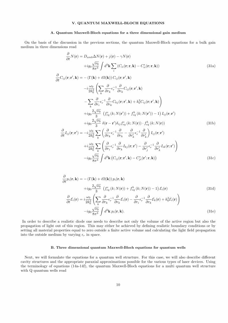
V. QUANTUM MAXWELL-BLOCH EQUATIONS

A. Quantum Maxwell-Bloch equations for a three dimensional gain medium

On the basis of the discussion in the previous sections, the quantum Maxwell-Bloch equations for a bulk gainmedium in three dimensions read

∂

∂tN(r) = Damb∆N(r) + j(r)− γN(r)

+ig0

√ν0

8π3

∫d3k

∑i

(Cii(r; r,k)− C∗ii(r; r,k)) (31a)

∂

∂tCij(r; r′,k) = − (Γ(k) + iΩ(k)) Cij(r; r′,k)

−iω0

2k20

(∑k

∂

∂rkε−1r

∂

∂rkCij(r; r′,k)

−∑

k

∂

∂riε−1r

∂

∂rkCkj(r; r′,k) + k2

0Cij(r; r′,k)

)

+ig02√

ν0

3(fe

eq (k; N(r′)) + fheq (k; N(r′))− 1

)Iij(r; r′)

+ig02√

ν0

3δ(r− r′)δijf

eeq (k; N(r)) · fh

eq (k; N(r)) (31b)

∂

∂tIij(r; r′) = −i

ω0

2k20

∑k

(∂

∂rkε−1r

∂

∂rk− ∂

∂r′kε−1r

∂

∂r′k

)Iij(r; r′)

+iω0

2k20

∑k

(∂

∂riε−1r

∂

∂rkIkj(r; r′)− ∂

∂r′jε−1r

∂

∂r′kIik(r; r′)

)

−ig0

√ν0

8π3

∫d3k

(Cij(r; r′,k)− C∗

ji(r′; r,k)

)(31c)

∂

∂tpi(r,k) = − (Γ(k) + iΩ(k)) pi(r,k)

+ig02√

ν0

3(fe

eq (k; N(r)) + fheq (k; N(r))− 1

) Ei(r) (31d)

∂

∂tEi(r) = i

ω0

2k20

(∑k

∂

∂rkε−1r

∂

∂rkEi(r)− ∂

∂riε−1r

∂

∂rkEk(r) + k2

0Ei(r)

)

−ig0

√ν0

8π3

∫d3k pi(r,k). (31e)

In order to describe a realistic diode one needs to describe not only the volume of the active region but also thepropagation of light out of this region. This may either be achieved by defining realistic boundary conditions or bysetting all material properties equal to zero outside a finite active volume and calculating the light field propagationinto the outside medium by varying εr in space.

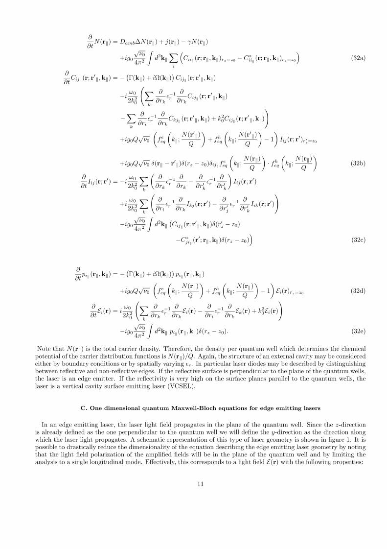
B. Three dimensional quantum Maxwell-Bloch equations for quantum wells

Next, we will formulate the equations for a quantum well structure. For this case, we will also describe differentcavity structures and the appropriate paraxial approximations possible for the various types of laser devices. Usingthe terminology of equations (14a-14f), the quantum Maxwell-Bloch equations for a multi quantum well structurewith Q quantum wells read

10

∂

∂tN(r‖) = Damb∆N(r‖) + j(r‖)− γN(r‖)

+ig0

√ν0

4π2

∫d2k‖

∑i

(Cii‖(r; r‖,k‖)rz=z0 − C∗

ii‖(r; r‖,k‖)rz=z0

)(32a)

∂

∂tCij‖(r; r

′‖,k‖) = − (Γ(k‖) + iΩ(k‖))Cij‖(r; r

′‖,k‖)

−iω0

2k20

(∑k

∂

∂rkε−1r

∂

∂rkCij‖ (r; r′‖,k‖)

−∑

k

∂

∂riε−1r

∂

∂rkCkj‖ (r; r′‖,k‖) + k2

0Cij‖(r; r′‖,k‖)

)

+ig0Q√

ν0

(fe

eq

(k‖;

N(r′‖)Q

)+ fh

eq

(k‖;

N(r′‖)Q

)− 1)

Iij(r; r′)r′z=z0

+ig0Q√

ν0 δ(r‖ − r′‖)δ(rz − z0)δij‖feeq

(k‖;

N(r‖)Q

)· fh

eq

(k‖;

N(r‖)Q

)(32b)

∂

∂tIij(r; r′) = −i

ω0

2k20

∑k

(∂

∂rkε−1r

∂

∂rk− ∂

∂r′kε−1r

∂

∂r′k

)Iij(r; r′)

+iω0

2k20

∑k

(∂

∂riε−1r

∂

∂rkIkj(r; r′)− ∂

∂r′jε−1r

∂

∂r′kIik(r; r′)

)

−ig0

√ν0

4π2

∫d2k‖

(Cij‖(r; r

′‖,k‖)δ(r′z − z0)

−C∗ji‖ (r′; r‖,k‖)δ(rz − z0)

)(32c)

∂

∂tpi‖(r‖,k‖) = − (Γ(k‖) + iΩ(k‖)

)pi‖(r‖,k‖)

+ig0Q√

ν0

(fe

eq

(k‖;

N(r‖)Q

)+ fh

eq

(k‖;

N(r‖)Q

)− 1)Ei(r)rz=z0 (32d)

∂

∂tEi(r) = i

ω0

2k20

(∑k

∂

∂rkε−1r

∂

∂rkEi(r) − ∂

∂riε−1r

∂

∂rkEk(r) + k2

0Ei(r)

)

−ig0

√ν0

4π2

∫d2k‖ pi‖(r‖,k‖)δ(rz − z0). (32e)

Note that N(r‖) is the total carrier density. Therefore, the density per quantum well which determines the chemicalpotential of the carrier distribution functions is N(r‖)/Q. Again, the structure of an external cavity may be consideredeither by boundary conditions or by spatially varying εr. In particular laser diodes may be described by distinguishingbetween reflective and non-reflective edges. If the reflective surface is perpendicular to the plane of the quantum wells,the laser is an edge emitter. If the reflectivity is very high on the surface planes parallel to the quantum wells, thelaser is a vertical cavity surface emitting laser (VCSEL).

C. One dimensional quantum Maxwell-Bloch equations for edge emitting lasers

In an edge emitting laser, the laser light field propagates in the plane of the quantum well. Since the z-directionis already defined as the one perpendicular to the quantum well we will define the y-direction as the direction alongwhich the laser light propagates. A schematic representation of this type of laser geometry is shown in figure 1. It ispossible to drastically reduce the dimensionality of the equation describing the edge emitting laser geometry by notingthat the light field polarization of the amplified fields will be in the plane of the quantum well and by limiting theanalysis to a single longitudinal mode. Effectively, this corresponds to a light field E(r) with the following properties:

11

Ex(r) := E0(rx)ξ(ry , rz) (33a)Ez(r) := 0 (33b)

∂

∂ryEy(r) := − ∂

∂rxEx(r). (33c)

The envelope function ξ(ry , rz) describes both the propagation along the y-direction and the confinement along thez-direction. It represents an approximate solution of the wave equation in the yz-plane normalized by∫

dry drz | ξ(ry , rz) |2= 1. (33d)

The equations are then limited to light field modes with the two dimensional envelope ξ(ry, rz). Spontaneous emissioninto other light field modes must be considered by including the rate of emission in the carrier recombination rateγ. Since the length L of the laser in the y-direction is also an important property of the device, it is included byconsidering the openness of the optical cavity. With the reflectivities of the laser mirrors given by R1 and R2, thelight field in the cavity is damped by losses through the mirrors at a rate of

κ = − c

2L√

εrln[R1R2]. (34)

The new one-dimensional variables are now defined as follows:

N1D(rx) =∫

dryN(r‖) (35a)

C0(rx; r′x,k‖) =∫

dry drz dr′yξ(ry , rz)ξ∗(r′y , r′z = z0)Cxx(r; r′‖,k‖) (35b)

I0(rx; r′x) =∫

dry drz dr′y dr′zξ(ry , rz)ξ∗(r′y , r′z)Ixx(r; r′) (35c)

p0(rx,k‖) =∫

dryξ∗(ry , rz = z0)px(r‖,k‖) (35d)

E0(rx) =∫

dry drzξ∗(ry , rz)Ex(r). (35e)

The carrier density is now given in terms of a one dimensional density. To obtain the two dimensional carrier densityper quantum well, this density is to be divided by QL. Note that the intensity is also given in terms of photons perunit length. The dynamics of the edge emitter then reads

∂

∂tN1D(rx) = Damb

∂2

∂r2x

N1D(rx) + Lj(rx)− γN1D(rx)

+ig0

√ν0

4π2

∫d2k‖

(C0(rx; rx,k‖)− C∗

0 (rx; rx,k‖))

(36a)

∂

∂tC0(rx; r′x,k‖) = − (Γ(k‖) + iΩ(k‖)

)C0(rx; r′x,k‖)

−κC0(rx; r′x,k‖)− iω0

2k20εr

∂2

∂r2x

C0(rx; r′x,k‖)

+ig0σ√

ν0

(fe

eq

(k‖;

N1D(r′x)QL

)+ fh

eq

(k‖;

N1D(r′x)QL

)− 1)

I0(rx; r′x)

+ig0σ√

ν0 δ(rx − r′x)feeq

(k‖;

N1D(rx)QL

)· fh

eq

(k‖;

N1D(rx)QL

)(36b)

∂

∂tI0(rx; r′x) = −2κI0(rx; r′x)− i

ω0

2k20εr

(∂2

∂r2x

− ∂2

∂r′2x

)I0(rx; r′x)

−ig0

√ν0

4π2

∫d2k‖

(C0(rx; r′x,k‖)− C∗

0 (r′x; rx,k‖))

(36c)

∂

∂tp0(rx,k‖) = − (Γ(k‖) + iΩ(k‖)

)p0(rx,k‖)

12

+ig0σ√

ν0

(fe

eq

(k‖;

N1D(rx)QL

)+ fh

eq

(k‖;

N1D(rx)QL

)− 1)E0(rx) (36d)

∂

∂tE0(rx) = −κE0(rx) + i

ω0

2k20εr

∂2

∂r2x

E0(rx)− ig0

√ν0

4π2

∫d2k‖ p0(rx,k‖), (36e)

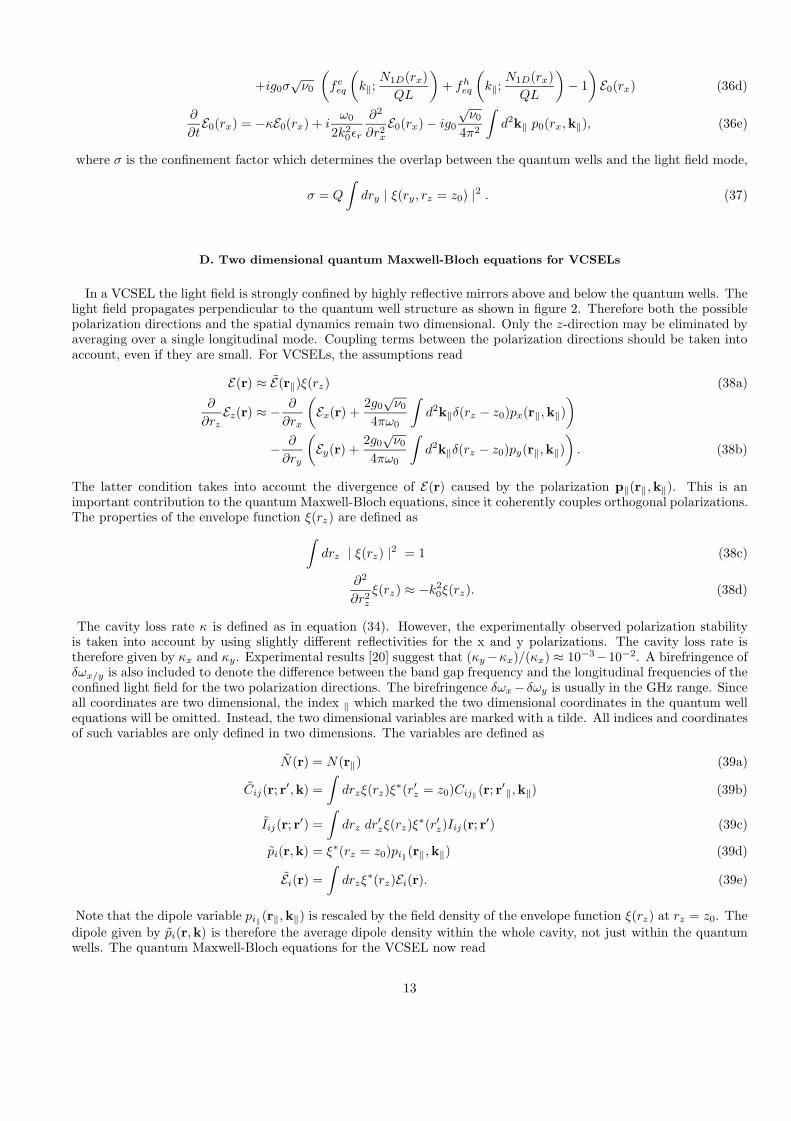
where σ is the confinement factor which determines the overlap between the quantum wells and the light field mode,

σ = Q

∫dry | ξ(ry, rz = z0) |2 . (37)

D. Two dimensional quantum Maxwell-Bloch equations for VCSELs

In a VCSEL the light field is strongly confined by highly reflective mirrors above and below the quantum wells. Thelight field propagates perpendicular to the quantum well structure as shown in figure 2. Therefore both the possiblepolarization directions and the spatial dynamics remain two dimensional. Only the z-direction may be eliminated byaveraging over a single longitudinal mode. Coupling terms between the polarization directions should be taken intoaccount, even if they are small. For VCSELs, the assumptions read

E(r) ≈ E(r‖)ξ(rz) (38a)

∂

∂rzEz(r) ≈ − ∂

∂rx

(Ex(r) +

2g0√

ν0

4πω0

∫d2k‖δ(rz − z0)px(r‖,k‖)

)− ∂

∂ry

(Ey(r) +

2g0√

ν0

4πω0

∫d2k‖δ(rz − z0)py(r‖,k‖)

). (38b)

The latter condition takes into account the divergence of E(r) caused by the polarization p‖(r‖,k‖). This is animportant contribution to the quantum Maxwell-Bloch equations, since it coherently couples orthogonal polarizations.The properties of the envelope function ξ(rz) are defined as∫

drz | ξ(rz) |2 = 1 (38c)

∂2

∂r2z

ξ(rz) ≈ −k20ξ(rz). (38d)

The cavity loss rate κ is defined as in equation (34). However, the experimentally observed polarization stabilityis taken into account by using slightly different reflectivities for the x and y polarizations. The cavity loss rate istherefore given by κx and κy. Experimental results [20] suggest that (κy−κx)/(κx) ≈ 10−3−10−2. A birefringence ofδωx/y is also included to denote the difference between the band gap frequency and the longitudinal frequencies of theconfined light field for the two polarization directions. The birefringence δωx− δωy is usually in the GHz range. Sinceall coordinates are two dimensional, the index ‖ which marked the two dimensional coordinates in the quantum wellequations will be omitted. Instead, the two dimensional variables are marked with a tilde. All indices and coordinatesof such variables are only defined in two dimensions. The variables are defined as

N(r) = N(r‖) (39a)

Cij(r; r′,k) =∫

drzξ(rz)ξ∗(r′z = z0)Cij‖ (r; r′‖,k‖) (39b)

Iij(r; r′) =∫

drz dr′zξ(rz)ξ∗(r′z)Iij(r; r′) (39c)

pi(r,k) = ξ∗(rz = z0)pi‖(r‖,k‖) (39d)

Ei(r) =∫

drzξ∗(rz)Ei(r). (39e)

Note that the dipole variable pi‖(r‖,k‖) is rescaled by the field density of the envelope function ξ(rz) at rz = z0. Thedipole given by pi(r,k) is therefore the average dipole density within the whole cavity, not just within the quantumwells. The quantum Maxwell-Bloch equations for the VCSEL now read

13

∂

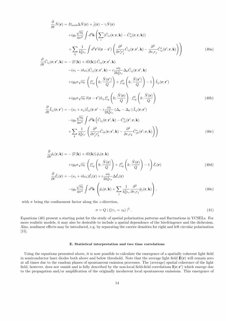
∂tN(r) = Damb∆N(r) + j(r)− γN(r)

+ig0

√ν0

4π2

∫d2k

(∑i

(Cii(r; r,k) − C∗ii(r; r,k))

+∑ij

1k20εr

∫d2r′δ(r− r′)

(∂2

∂r′ir′j

Cij(r; r′,k)− ∂2

∂rirjC∗

ij(r′; r,k)

) (40a)

∂

∂tCij(r; r′,k) = − (Γ(k) + iΩ(k)) Cij(r; r′,k)

−(κi − iδωi)Cij(r; r′,k)− iω0

2k20εr

∆rCij(r; r′,k)

+ig0σ√

ν0

(fe

eq

(k;

N(r′)Q

)+ fh

eq

(k;

N(r′)Q

)− 1

)Iij(r; r′)

+ig0σ√

ν0 δ(r − r′)δijfeeq

(k;

N(r)Q

)· fh

eq

(k;

N(r)Q

)(40b)

∂

∂tIij(r; r′) = −(κi + κj)Iij(r; r′ − i

ω0

2k20εr

(∆r −∆r′) Iij(r; r′)

−ig0

√ν0

4π2

∫d2k

(Cij(r; r′,k)− C∗

ji(r′; r,k)

+∑

k

1k20εr

(∂2

∂r′jr′k

Cik(r; r′,k)− ∂2

∂rirkC∗

jk(r′; r,k)

))(40c)

∂

∂tpi(r,k) = − (Γ(k) + iΩ(k)) pi(r,k)

+ig0σ√

ν0

(fe

eq

(k;

N(r)Q

)+ fh

eq

(k;

N(r)Q

)− 1

)Ei(r) (40d)

∂

∂tEi(r) = −(κi + iδωi)Ei(r) + i

ω0

2k20εr

∆Ei(r)

−ig0

√ν0

4π2

∫d2k

pi(r,k) +∑

j

1k20εr

∂2

∂rirjpj(r,k)

, (40e)

with σ being the confinement factor along the z-direction,

σ = Q | ξ(rz = z0) |2 . (41)

Equations (40) present a starting point for the study of spatial polarization patterns and fluctuations in VCSELs. Formore realistic models, it may also be desirable to include a spatial dependence of the birefringence and the dichroism.Also, nonlinear effects may be introduced, e.g. by separating the carrier densities for right and left circular polarization[15].

E. Statistical interpretation and two time correlations

Using the equations presented above, it is now possible to calculate the emergence of a spatially coherent light fieldin semiconductor laser diodes both above and below threshold. Note that the average light field E(r) will remain zeroat all times due to the random phases of spontaneous emission processes. The (average) spatial coherence of the lightfield, however, does not vanish and is fully described by the non-local field-field correlations I(r; r′) which emerge dueto the propagation and/or amplification of the originally incoherent local spontaneous emissions. This emergence of

14

coherence as a concequence of incoherent emissions has been discussed in a temporal context using nonequilibriumGreen’s functions in [11].

In order to understand the physical implications of the well known absence of an average light field in lasers, itshould be recalled that all the results of the quantum Maxwell-Bloch equations represent averages which have to beinterpreted in terms of statistical physics. For example, the field-field correlation I(r; r′) represents a variance of theprobability distribution with respect to the possible spatial electromagnetic field values. The coherent field observedin experimental time-resolved measurements will vary randomly from measurement to measurement according to thisprobability distribution. Indeed, the intensity distribution itself will vary depending on the random phase interferenceof the eigenmodes given by I(r; r′). The calculated average spatial intensity distribution I(r; r) only describes theaverage near field pattern, which is likely to be close to but not identical with the one actually observed. Thefluctuations of the actual intensity distribution around this average, however, are disregarded as a consequence of thefactorization performed in section II. Moreover, the fluctuations in the carrier density distribution induced by spatialholeburning associated with these fluctuations of the intensity distribution have also been disregarded.

While the average spatial coherence of the light field is fully described by the quantum Maxwell-Bloch equations,the average expected temporal coherence has not yet been explicitly considered. Indeed, it is not necessary to considertemporal coherence in the closed sets of quantum Maxwell-Bloch equations given above because all the informationrequired to obtain the correct emission and absorption rates are incorporated in the field-dipole correlation C(r; r′,k).As shown in section VI, the spectra of gain and spontaneous emission are implicitly given by the coherent dipoledynamics which enters into the temporal evolution of this field-dipole correlation. If explicit information about thetwo time correlations is desired, however, such correlations may be included in the dynamics by noting that thetemporal evolution of the two time correlations of the field I(r, t; r′, t′) and the two time correlations of the field-dipole correlation C(r, t; r′,k, t′) is equivalent to the dynamics of the field and dipole expectation values [25]. Whilethe quantum Maxwell-Bloch equations for the correlations at t = t′ remain unchanged, the evolution of the two timecorrelations as a function of t′ > t is then given by an additional pair of equations which depend on the carrierdynamics given by the solution of the original system of quantum Maxwell-Bloch equations as presented above. Inthe case of VCSELs these additional equations supplementing equations (40) read

∂

∂t′Cij(r, t; r′,k, t′) = − (Γ(k) + iΩ(k)) Cij(r, t; r′,k, t′)

+ig0σ√

ν0

(fe

eq

(k;

N(r, t′)Q

)+ fh

eq

(k;

N(r, t′)Q

)− 1

)Iij(r, t; r′, t′) (42a)

∂

∂t′Iij(r, t; r′, t′) = −(κj + iδωj)Iij(r, t; r′, t′) + i

ω0

2k20εr

∆r′ Iij(r, t; r′, t′)

−ig0

√ν0

4π2

∫d2k Cij(r, t; r′,k, t′)

−ig0

√ν0

4π2

∫d2k

∑k

1k20εr

∂2

∂r′jr′k

Cik(r, t; r′,k, t′). (42b)

If the carrier density changes slowly, the equations describe the linear response of the medium caused by the initialintensity distribution Iij(r, t; r′, t) and the initial field-dipole correlation Cij(r, t; r′,k, t) determined from equations(40). In this case it is possible to derive the spectrum and the gain from the eigenmodes and the associated eigenvaluesof the quasi-stationary linear optical system. Note that the eigenmodes of the linearized dynamics are not necessarilyidentical with the eigenmodes of the intensity distribution Iij(r, t; r′, t), since fast variations in the carrier densitydistribution may have induced phase locking between the dynamical eigenmodes.

In general, the frequency spectra of the light field are given by Fourier transforms of the two-time correlationsobtained from equations (42). However, as noted above, such spectra do not comprise any effects which arise fromcarrier density fluctuations. These effects are known to be quite significant. Well known examples of carrier fluctu-ation effects in the frequency spectrum of semiconductor lasers are the linewidth enhancement phenomenologicallydescribed by the linewidth enhancement factor α and the relaxation oscillation sidebands observed in stable singlemode operation. Moreover, spatial carrier density fluctuations may also significantly modify the multi mode spectraof semiconductor laser devices, as pointed out recently for the case of semiconductor laser arrays [24].

15

VI. AMPLIFIED SPONTANEOUS EMISSION PROPERTIES: ANALYTICAL RESULTS OF THEQUANTUM MAXWELL-BLOCH EQUATIONS

A. Gain and spontaneous emission

For a given carrier distribution fe/h(k), the dynamics of the optical field E(r) and the dipole density p(r) are linear.In this case, it is possible to integrate the equations of motion to obtain a Green’s function for the field dynamics.The equation for bulk material reads

∂

∂tE(r, t)

∣∣∣∣cL

= g20

ν0

12π3

∫d3k

∫ ∞

0

dτ e−(Γ(k)+iΩ(k))τ

× (fe(k) + fh(k)− 1)E(r, t− τ). (43a)

Correspondingly, the equation for a multi quantum well structure of Q quantum wells has the form

∂

∂tE(r, t)

∣∣∣∣cL

= g20

Qν0

4π2δ(rz − z0)

∫d2k‖

∫ ∞

0

dτ e−(Γ(k‖)+iΩ(k‖))τ

× (fe(k‖) + fh(k‖)− 1)E(r, t − τ). (43b)

An expression for the rate G(ω) at which a light field mode of frequency ω is amplified can be derived by solvingthe integral over τ using E(r, t − τ) ≈ eiωτE(r, t). The real part of the result is the gain spectrum given in terms ofamplification per unit time, G(ω). For bulk material, this amplification rate is given by

Gbulk(ω) = g20

ν0

12π3

∫d3k

Γ(k)Γ2(k) + (Ω(k) − ω)2

(fe(k) + fh(k)− 1

), (44a)

and for quantum wells, the corresponding amplification rate reads

GQW (ω) = g20

Qν0

4π2δ(rz − z0)

∫d2k‖

Γ(k‖)Γ2(k‖) + (Ω(k‖)− ω)2

(fe(k‖) + fh(k‖)− 1

). (44b)

The gain per unit length can be obtained by dividing the rate G(ω) by the speed of light in the semiconductormedium, cε

−1/2r . However, in order to establish the connection between the gain spectrum and the spectral density

of spontaneous emission, it is more convenient to use the amplification rate as a starting point.The quantum Maxwell-Bloch equations for the field-dipole correlation Cij(r; r′,k) show that the ratio between the

spontaneous contributions and the stimulated contributions is

∂∂tCij(r; r′,k)

∣∣spontaneous

∂∂tCij(r; r′,k)

∣∣stimulated

=δ(r− r′)δijf

e(k) · fh(k)Iij(r; r′) (fe(k) + fh(k)− 1)

. (45)

In this equation, δ(r − r′)δij corresponds to a photon density of one photon per mode. The spectral density of thespontaneous emission may therefore be obtained by replacing (fe(k)+fh(k)−1) with fe(k) ·fh(k) in equations (44a)and (44b), respectively, and multiplying the resulting rates with twice the density of light field modes which couple tothe medium (the factor of two being a result of considering intensities instead of fields). At the band edge frequencyω0, the density of light field modes per volume and frequency interval in a continuous medium is

ρlight =ω2

0

π2c3ε3/2r . (46)

The density of the spontaneous emission rate for bulk material Sbulk(ω) thus reads

Sbulk(ω) = ρlightg20

ν0

6π3

∫d3k

Γ(k)Γ2(k) + (Ω(k)− ω)2

fe(k) · fh(k). (47a)

For quantum wells, the density of modes is only 2/3 of ρlight, since the dipole component perpendicular to thequantum well is zero. Also, the delta function δ(rz − z0) may be omitted to obtain the emission density per area. Thespontaneous emission density SQW (ω) is then given by

16

SQW (ω) =23ρlightg

20

Qν0

2π2δ(rz − z0)

∫d2k‖

Γ(k‖)Γ2(k‖) + (Ω(k‖)− ω)2

fe(k‖) · fh(k‖). (47b)

The total rate of spontaneous emission per unit volume or area may be obtained by integrating over all frequencies.This integral removes the dependence on Γ(k). For bulk material,∫

dω Sbulk(ω) = ρlight g20

ν0

6π2

∫d3k fe(k) · fh(k) (48a)

and for quantum wells, ∫dω SQW (ω) = ρlight g2

0

Qν0

3πδ(rz − z0)

∫d2k‖ fe(k‖) · fh(k‖). (48b)

For zero temperature, the spontaneous emission rate may be derived by noting that fe(k) · fh(k) = fe(k) = fh(k).The integral over k may thus be solved, resulting in∫

d3k fe(k) · fh(k) = 4π3N (49a)

for bulk material and ∫d2k‖ fe(k‖) · fh(k‖) =

2π2

QN (49b)

for quantum wells. For both bulk and quantum wells the density of spontaneous emission now may be expressed as

Stotal =N

τs, (50)

where 1/τs is the rate of spontaneous emission given by

1τs

=2π

3ρlightg

20ν0. (51)

Using equation (30), the rate of spontaneous emission may also be expressed in terms of the dipole matrix elementdcv,

1τs

=4

hω0ε1/2r

14πε0

ω40

3c3| dcv |2

=4

hω0Prad, (52)

where Prad is the classical power radiated by an oscillating dipole of the amplitude dcv. Note that the factor of4/hω0 is consistent with a quantum noise interpretation of spontaneous emission such as the one represented bythe semiclassical Langevin equations. According to this interpretation, the fluctuations of each dipole are given by2 | dcv |2 because both the real and the imaginary part of the dipole contribute. The spontaneous emission of anexcited atom is then composed of one half amplified field noise and one half dipole fluctuations. Therefore, each one ofthe two dipole components contributes one quarter of the total spontaneous emission of an excited state. Numericalvalues of | dcv | and g0 for GaAs may be determined by assuming a spontaneous lifetime of τs = 3 ns, a band gap ofhω0 = 1.5 eV and εr = 12. The dipole matrix element is then | dcv |= 4.3×10−29Cm which corresponds to a distanceof 2.7× 10−10m times the electron charge and the coupling frequency is g0 = 2.1× 1015s−1.

For quantum wells at zero temperature, the integrals over k‖ can be solved analytically using equation (20) andassuming that Γ is independent of k‖. The resulting gain spectrum is then given by

ε1/2r

cGQW (ω) =

ε1/2r

cg20

Qν0

2πh

meeffmh

eff

meeff + mh

eff

δ(rz − z0)(

2 arctan(

Ωf − ω

Γ

)+ arctan

(ω

Γ

)− π

2

), (53)

where Ωf is the transition frequency at the Fermi surface of the electrons and holes. It is related to the carrier densityN by

17

Ωf =πh

Q

meeff + mh

eff

meeffmh

eff

N. (54)

The spectral density of spontaneous emission is thus given by

SQW (ω) = ρlightg20

2Qν0

3πh

meeffmh

eff

meeff + mh

eff

(arctan

(Ωf − ω

Γ

)+ arctan

(ω

Γ

)). (55)

Typical spectra of gain and spontaneous emission of an active layer containing Q = 5 quantum wells obtained fromthe analytic approximations (53) and (55), respectively, are presented in Fig. 3 for characteristic values of the carrierdensity. For the spectra in Fig. 3 we have assumed a total spontaneous emission lifetime of τs = 3 ns and a band gapof hω0 = 1.5 eV. Other parameters are the effective mass of electrons (me

eff = 0.067m0) and holes (mheff = 0.053m0),

given in units of the electron mass m0 as well as the dipole damping rate hΓ = 8 meV, and dielectric constantεr = 12. Gain and spontaneous emission are both displayed relative to the peak values Smax = 2.7 × 107cm−2 andGmax = 2.5 × 107cms−1δ(rz − z0). The gain value may be interpreted by calculating the gain of a light beam ofwidth σ−1 = 10−5 cm with an incidence perpendicular with respect to the quantum well and traveling at a speed of1010cms−1 in the plane of the quantum well. The maximal gain is then given by 250cm−1. The five spectra displayedin Fig. 3 are the gain at N = 0 (g0), the gain at N = 1012cm−2 (g1), the spontaneous emission at N = 1012cm−2

(s1), the gain at N = 5 × 1012cm−2 (g5) and the spontaneous emission at N = 5 × 1012cm−2 (s5). Fig. 3 clearlyshows the influence of the carrier density N . In the absence of charge carriers (g0), the laser is purely absorptive.With increasing carrier density N , transparency is reached at N = 1012cm−2 (g1). This density is characterized byvanishing gain (i.e. there is neither gain nor absorption) at a frequency of hω = 0. At the same time, however, thereis a significant contribution of spontaneous emission (s1) with a maximum at a frequency of hω ≈ 4 meV. Finally, athigh values of the carrier density (N = 5×1012cm−2), both gain (g5) and spontaneous emission (s5) have a maximumabove the band-gap frequency.

B. Spontaneous emission factor and far field pattern of an edge emitting laser

In the optical cavity of a laser the equations for gain and spontaneous emission are modified by the mode structure.In particular, the total linear response of an electromagnetic field mode inside the cavity includes the cavity loss rateκ. For the edge emitting semiconductor laser, the gain function of the cavity modes is given by

G1D(ω) = g20

ν0

4π2σ

∫d2k‖

Γ(k‖) + κ

(Γ(k‖) + κ)2 + (Ω(k‖)− ω)2(fe(k‖) + fh(k‖)− 1

), (56)

where the confinement factor σ is defined according to equation (37). Spontaneous emission into the cavity modespasses through the gain medium and is thereby absorbed or amplified accordingly. Thus for an edge emitting laser,the rate of spontaneous emission into a cavity mode of frequency ω is given by

S1D(ω) = 2g20

ν0

4π2σ

∫d2k‖

Γ(k‖) + κ

(Γ(k‖) + κ)2 + (Ω(k‖)− ω)2fe(k‖) · fh(k‖). (57)

This rate represents the total rate of spontaneous emission events per mode, regardless of the actual width of thelaser. On the other hand, equation (50) gives the total rate of spontaneous emission per quantum well area.

1. Spontaneous emission factor

In a laser of length L and total width W (c.f. Fig. 1), the spontaneous emission rate into free space is LW Stotal.The spontaneous emission factor β, which is generally defined as the fraction of spontaneous emission being emittedinto the cavity mode [2], is on the basis of our theory given by the expression

β(ω, N1D) =τsS1D

W N1D. (58)

Note that the two dimensional carrier density N in the quantum well is related to the one dimensional carrierdensity N1D by N1D = L N . The spontaneous emission factor β is a function of both frequency and carrier density.

18

Consequently, the common assumption of the spontaneous emission factor β being independent of the carrier density[2,7] may be regarded as an approximation similar to the assumption of linear gain.

An analytical expression for the spontaneous emission factor may be obtained for zero temperature. The k-spaceintegrals may then be solved analytically using equation (20) and assuming that Γ is independent of k‖. For thespontaneous emission factor β, the analytical result reads

β(ω, Ωf ) =3σ

2πρlightQ W L Ωf

(arctan

(Ωf − ω

Γ + κ

)+ arctan

(ω

Γ + κ

)). (59)

The Fermi frequency Ωf is defined by equation(54) and expresses, in particular, the carrier density dependence of β.For Ωf , ω Γ+κ we recover the result typically given in the literature (e.g. [2]) which does not depend on N . Fig. 4shows the deviation of the spontaneous emission factor from this value as the Fermi frequency Ωf passes the point ofresonance with the cavity mode. Fig. 4 illustrates, in particular, the carrier density dependence of β for three modeswith frequencies above the band gap frequency given by (a) ω = 0, (b) ω = 0.5(Γ + κ), and (c) ω = Γ + κ. Mostnotably, β is always smaller than the usual estimate given by β(ω = Ωf = 0), which is based on the assumption ofideal resonance between the transition frequency and the cavity mode.

2. Far-field pattern of a broad area laser

With equations (56) and (57), it is possible to find the steady state intensity Is of a mode with frequency ω,

Is(ω) =S1D(ω)

2κ− 2G1D(ω). (60)

Note that this result may also be obtained directly from equations (36a-36e). In a wide cavity, the cavity modes areapproximately plane wave modes and the relation between I0(ω) and I0(rx; r′x) in that case reads

I0(rx, r′x) =∫

dq eiq(rx−r′x) I

(ω =

ω0q2

2k20εr

). (61)

The steady state intensity distribution is characterized by the spatial coherence derived from the intensity distributionof the plane wave modes of the cavity. Generally, the intensity distribution of plane waves corresponds in the far fieldto an optical field at angles relative to the axis of emission in the plane of the quantum well. The angular distributionof intensity and coherence in the far field is thus given by

If (Θ, Θ′) =k0

2π

∫drxdr′x eik0ΘrxI0(rx, r′x)e−ik0Θ′r′x . (62)

Therefore, the far field intensity distribution may be determined directly from the frequency dependence of theintensities by

If (Θ, Θ) = Wk0 Is

(ω =

ω0Θ2

2εr

), (63)

the intensity is given in units of 2κhω0 per unit angle.For T = 0 we may in analogy to (59) solve the integral in (57) by assuming Γ to be independent of k. As an

analytical expression we then obtain for the far-field intensity distribution of a broad area semiconductor laser

If (Θ, Θ) = Wk0

arctan(

Ωf−ω(Θ)Γ+κ

)+ arctan

(ω(Θ)Γ+κ

)π(R + 1

2 )− 2 arctan(

Ωf−ω(Θ)Γ+κ

)− arctan

(ω(Θ)Γ+κ

) ,

with R =2hκ

g20ν0σ

meeff + mh

eff

meeffmh

eff

and ω(Θ) =ω0Θ2

2εr. (64)

The parameter R represents the ratio between the cavity loss rate κ and the maximum amplification rate of the gainmedium. Laser activity is only possible if R < 1. The classical laser threshold is defined by the carrier density for

19

which the denominator of If (Θ, Θ) is zero for a single specific frequency ω(Θ). Consequently, the carrier density atwhich this occurs is pinned. Figure 5 shows the far field intensity distribution for different carrier densities below thispinning density. In Fig. 5 (a), the wide intensity distribution of amplified spontaneous emission for carrier densitiesis much lower than the pinning density. The intensity maximum is clearly located at Θ = 0. Figure 5(a) shows theintensity distribution for carrier densities halfway towards threshold. Already, the intensity maxima move to anglesof ±15, corresponding to the frequency at which the gain spectrum has its maximum. In the case of Fig. 5(c), thethreshold region is very close to the pinning density. The peaks in the far field pattern narrow as the laser intensityis increased. Consequently the far field pattern indeed is a measure of the spatial coherence – similar as the linewidthof the laser spectrum is a measure of temporal coherence. It is therefore desirable to consider quantum noise effectsin the spatial patterns of optical systems. In the context of squeezing, such patterns have been investigated by Gattiand coworkers [26] based on the general formulation of Lugiato and Castelli [27]. The laser patterns presented hereare based on the same principles. Usually, however, the strong dissipation prevents squeezing in laser systems unlessthe pump-noise fluctuations are suppressed [28].

VII. CONCLUSIONS

The quantum Maxwell-Bloch equations (QMBE) for spatially inhomogeneous semiconductor lasers derived in thispaper take into account the quantum mechanical nature of the light field as well as that of the carrier system. Theonly approximation used in the derivation of the intensity and correlation dynamics is that of statistical indepen-dence between the two carrier systems and the light field. In the QMBE presented here, the effects of coherentspatiotemporal quantum fluctuations which are generally not considered in the semiclassical Maxwell-Bloch equationsfor semiconductor laser devices have thus been taken into account.

The spontaneous emission term appears side by side with the gain and absorption term in the dynamics of the field-dipole correlation. In this way the spatial coherence of spontaneous emission and amplified spontaneous emission isconsistently described by the quantum Maxwell-Bloch equations. Typical features of the model have been illustratedby the spectra of gain and spontaneous emission. An example of the spatial coherence characteristics describedby the quantum Maxwell-Bloch equations has been presented by analytically obtaining the spontaneous emissionfactor β and the far field distribution for the example of a broad area edge emitting laser. In general the quantumMaxwell-Bloch equations derived for edge emitting and vertical cavity surface emitting lasers provide a starting pointfor a detailed analysis of spatial coherence patterns in diverse semiconductor laser geometries such as broad area orultra-low threshold lasers.

APPENDIX A: STOCHASTIC SIMULATION OF MEASUREMENTS

As explained at the end of section V, the field average of zero is an expression of our lack of knowledge about theactual physical field present in the laser device. This lack of knowledge could be removed by performing a measurementon the light field. For example, the phase information could be obtained by measuring the interference of the light fieldfrom the diode with light from a separate laser. A simple theoretical simulation of such a measurement is obtained byassuming that I(r; r′) defines the variance of a Gaussian distribution of coherent states (Gaussian P representation).The measurement of the actual field E(r) may then be simulated by randomly selecting a coherent field from thisGaussian distribution. Since the field and the dipole density are correlated, the statistical selection of E(r) shifts thedipole density average p(r,k) from zero to

p(r,k) =∫

dr′E(r)C(r′; r,k)∑ij

∫dr′Iij(r′; r′)

. (A1)

Because the field has been determined with a precision equal to the quantum limit, the correlations factorize and thenew values of I(r; r′) and C(r; r′,k) are given by the respective products of E(r) and p(r,k).

The drastic changes in the intensity distribution and in the dipole dynamics which may result from such a simulatedmeasurement cause spatial holeburning and give rise to relaxation oscillations. By performing several stochasticalsimulations starting from the same initial probability distribution, the statistics of the carrier density fluctuationsmay be obtained. It is then possible to derive the correct linewidth enhancement factor α as well as the relaxationoscillation sidebands directly from the dynamics of the quantum Maxwell-Bloch equations.

20

APPENDIX B: LANGEVIN EQUATIONS

An alternative approach to the problem of quantum noise is given by the Langevin equations [25,?]. Langevinequations simulate quantum noise by adding classical noise sources which reproduce the statistical properties givenby the uncertainty relations. In particular, the exponential damping terms given by the cavity loss rate κ and thedipole relaxation rate Γ must be compensated by a noise input maintaining the quantum fluctuations in the field anddipole densities. For quantum well lasers, these fluctuations are given by

〈E∗i (r)Ej(r)〉 =12δijδ(r− r′) (B1a)

〈p∗i‖(r‖,k‖)pj‖(r′‖,k′‖)〉 =

12δi‖j‖δ(r‖ − r′‖)4π2

(fe

eq

(k‖, N(r‖)

) · fheq

(k‖, N(r‖)

)+(1− fe

eq

(k‖, N(r‖)

)) · (1− fheq

(k‖, N(r‖)

))). (B1b)

Note that the variables Ei(r) and p(r‖,k‖) are classical quantities in this context. The Langevin equations pre-sented in the following do not describe quantum mechanical coherent states. Instead, semiclassical light fields anddipole densities are calculated with a precision violating the uncertainty relations. While the statistics thus derivedcorrespond to the quantum statistics, the theory applied is fully classical.

For a VCSEL, the semiclassical Langevin equations corresponding to the quantum Maxwell-Bloch equations (40read

∂

∂tN(r) = Damb∆N(r) + j(r)− γN(r)

+ig0

√ν0

4π2

∫d2k

(∑i

(E∗i (r)pi(r,k)− Ei(r)p∗i (r,k))

+∑ij

1k20εr

(E∗i (r)

∂2

∂rirjpj(r,k) − Ei(r)

∂2

∂rirjp∗j (r,k)

) (B2a)

∂

∂tpi(r,k) = − (Γ(k) + iΩ(k)) pi(r,k)

+ig0σ√

ν0

(fe

eq

(k;

N(r)Q

)+ fh

eq

(k;

N(r)Q

)− 1

)Ei(r) + qp

i (r,k, t) (B2b)

∂

∂tEi(r) = −(κi + iδωi)Ei(r) + i

ω0

2k20εr

∆Ei(r)

−ig0

√ν0

4π2

∫d2k

pi(r,k) +∑

j

1k20εr

∂2

∂rirjpj(r,k)

+ qEi (r, t) (B2c)

with the noise input terms qpi (r,k, t) and qEi (r, t) given by

〈qpi∗(r,k, t)qp

j (r′,k, t + τ)〉 = δ(τ)Γ(k)δijδ(r− r′)4π2σ(fe

eq

(k, N(r)

)· fh

eq

(k, N(r)

)+(1− f e

eq

(k, N(r)

))·(1− fh

eq

(k, N(r)

)))(B3a)

〈qEi∗(r, t)qEi (r′, t + τ)〉 = δ(τ)κδ(r − r′). (B3b)

These Langevin equations allow a stochastical simulation of quantum noise in a semiclassical context. However, it isnecessary to perform a large number of runs before statistical results can be obtained. In particular, the unrealisticintensity fluctuations of the light field vacuum need to average out before the results are consistent with quantumtheory.

21

[1] O. Hess and T. Kuhn, Prog. Quant. Electr. 20, 85 (1996).[2] K.J. Ebeling, Integrated Optoelectronics (Springer, Berlin 1993).[3] T. Lee, C.A. Burrus, J.A. Copeland, A.G. Dentai and D. Marcuse, IEEE J. Quantum Electron. QE-18, 1101 (1982).[4] K. Petermann, IEEE J. Quantum Electron. QE-15, 566 (1979).[5] A. Yariv and S. Margalit, IEEE J. Quantum Electron. QE-18, 1831 (1982).[6] A.E. Siegmann in coherence and Quantum Optics VII edited by Eberly, Mandel and Wolf (Plenum, New York 1996).[7] G. Bjork, A. Karlsson, and Y. Yamamoto, Phys. Rev. A 50, 1675 (1994).[8] Y. Yamamoto and R.E. Slusher, Physics Today, June 1993, 66 (1993).[9] F.Jahnke, K.Henneberger, W.Schafer and S.W. Koch, J.Opt.Soc.Am. B 10, 2394 (1993).

[10] F.Jahnke and S.W. Koch, Phys. Rev. A 52, 1712 (1995).[11] K. Henneberger and S.W. Koch, Phys. Rev. Lett. 76, 1820 (1996).[12] O. Hess and T. Kuhn, Phys. Rev. A 54, 3347 (1996).[13] P.Y. Yu and M. Cardona, Fundamentals of Semiconductors, (Springer, Berlin 1996).[14] E. Wigner, Phys. Rev. 40, 749 (1932).[15] M. San Miguel, Q. Feng and J.V. Moloney, Phys. Rev. A 52, 1728 (1995).[16] J. Martin-Regalado, M. San Miguel, N.B. Abraham and F. Prati, Opt. Lett 21, 351 (1995).[17] H.F. Hofmann and O. Hess, Phys. Rev. A 56, 868 (1997).[18] H. van der Lem and D. Lenstra, Opt. Lett. 22, 1698 (1997).[19] H.F. Hofmann and O. Hess, Quantum Semiclass. Opt. 10, 87 (1998).[20] A.K.J. van Doorn, M.P. van Exter, A.M. van der Lee and J.P. Woerdman, Phys. Rev. A 55, 1473 (1997).[21] W.W. Chow, S.W. Koch, and M. Sargent, Semiconductor-Laser Physics, (Springer, Berlin 1994).[22] T. Kuhn and F. Rossi, Phys. Rev. Lett. 69, 977 (1992), ibid., Phys. Rev. B 46, 7496 (1992).[23] C. Ell, R. Blank, S. Benner and H.Haug, J.Opt.Soc.Am. B 6, 2006 (1989).[24] H.F. Hofmann and O. Hess, Opt. Lett. 23, 391 (1998).[25] D.F. Walls and G.J. Milburn, Quantum Optics (Springer, Berlin 1994).[26] A. Gatti, H. Wiedemann, L.A. Lugiato, I.Marzoli, G. Oppo, and S.M.Barnett, Phys.Rev. A 56, 877 (1997).[27] L.Q. Lugiato and F. Castelli, Phys. Rev. Lett. 68, 3284 (1992).[28] Y. Yamamoto, S. Machida and O. Nilsson, Phys. Rev. A 34, 4025 (1986).

FIG. 1. Schematic representation of the edge emitter geometry. The laser field is mostly confined to the plane of the quantumwell and propagates along the y-axis.

FIG. 2. Schematic representation of a typical VCSEL geometry. The laser filed propagates perpendicularly to the quantumwell along the z-axis. The length of the optical resonator approximately corresponds to the wavelenth.

FIG. 3. Spectra of gain and spontaneous emission for a quantum well structure of Q = 5 quantum wells given relative toGmax = 2.5 × 107cms−1δ(rz − z0) and Smax = 2.7 × 107cm−2. The five spectra shown are the gain at N = 0 (g0), the gain atN = 1012cm−2 (g1), the spontaneous emission at N = 1012cm−2 (s1), the gain at N = 5× 1012cm−2 (g5) and the spontaneousemission at N = 5× 1012cm−2 (s5).

FIG. 4. Carrier density dependence of the spontaneous emission factor β for three modes with frequencies above the bandgap frequency given by (a) ω = 0, (b) ω = 0.5(Γ + κ), and (c) ω = Γ + κ. β0 = β(ω = N = 0) is determined by the geometryof the laser. The carrier density is given in terms of the transition frequency at the Fermi edge Ωf .

FIG. 5. Far field intensity distributions for R = 0.5, hω0 = 1.5 eV, h(Γ + κ) = 8 meV and εr = 12. The density is pinnedat Ωf = 1.8805(Γ + κ). Figure (a) shows the far field pattern for carrier densities of 0.05, 0.10 and 0.15 times pinning density,figure (b) shows the distribution for 0.25, 0.5. and 0.75 times pinning density and figure (c) shows the distribution for 0.90,0.95 and 0.99 times pinning density. The peaks appear at emission angles of ±15.

22