Quantum Fourier Transform to Estimate DriveCyclesVinayak Dixit  ( v.dixit@unsw.edu.au )

UNSW SydneySisi Jian 

the Hong Kong University of Science and Technology

Research Article

Keywords: Drive cycles, Quantum Fourier Transform, vehicle systems, energy consumption, emissions

Posted Date: August 4th, 2021

DOI: https://doi.org/10.21203/rs.3.rs-772223/v1

License: This work is licensed under a Creative Commons Attribution 4.0 International License.  Read Full License

Version of Record: A version of this preprint was published at Scienti�c Reports on January 13th, 2022.See the published version at https://doi.org/10.1038/s41598-021-04639-0.

Quantum Fourier Transform to Estimate Drive Cycles

Vinayak Dixita*, Sisi Jianb

a Research Centre for Integrated Transport Innovation (rCITI), School of Civil and Environmental

Engineering, UNSW Sydney

b Department of Civil and Environmental Engineering, the Hong Kong University of Science and

Technology, Clear Water Bay, Kowloon, Hong Kong SAR, China

*Corresponding author, Tel: (+61 2) 9385 5721, Email: v.dixit@unsw.edu.au

Quantum Fourier Transform to Estimate Drive Cycles

Abstract

Drive cycles in vehicle systems are important determinants for energy consumption, emissions, and

safety. Estimating the frequency of the drive cycle quickly is important for control applications related to

fuel efficiency, emission reduction and improving safety. Quantum computing has established the

computational efficiency that can be gained. A drive cycle frequency estimation algorithm based on the

quantum Fourier transform is exponentially faster than the classical Fourier transform. The algorithm is

applied on real world data set. We evaluate the method using a quantum computing simulator,

demonstrating remarkable consistency with the results from the classical Fourier Transform. Current

quantum computers are noisy, a simple method is proposed to mitigate the impact of the noise. The

method is evaluated on a 15 qbit IBM-q quantum computer. The proposed method for a noisy quantum

computer is still faster than the classical Fourier transform.

1. Introduction

Drive cycles are important determinants of emissions, energy consumption and safety. Higher

frequencies of acceleration and deceleration cycles are predictors of higher emissions, fuel consumption

(Ligterink et al. 2012) and crashes (Dixit et al., 2011; Dixit, 2013). Regulators, vehicle manufacturers and

traffic engineers are extremely interested to understand the driving cycles for implementing policies and

real-time control systems.

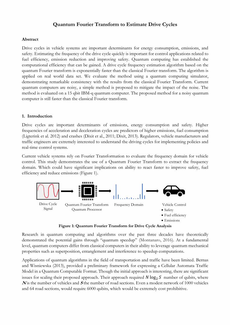
Current vehicle systems rely on Fourier Transformation to evaluate the frequency domain for vehicle

control. This study demonstrates the use of a Quantum Fourier Transform to extract the frequency

domain. Which could have significant implications on ability to react faster to improve safety, fuel

efficiency and reduce emissions (Figure 1).

Figure 1: Quantum Fourier Transform for Drive Cycle Analysis

Research in quantum computing and algorithms over the past three decades have theoretically

demonstrated the potential gains through “quantum speedup” (Montanaro, 2016). At a fundamental

level, quantum computers differ from classical computers in their ability to leverage quantum mechanical

properties such as superposition, entanglement and interference to speedup computations.

Applications of quantum algorithms in the field of transportation and traffic have been limited. Bernas

and Wisniewska (2013), provided a preliminary framework for expressing a Cellular Automata Traffic

Model in a Quantum Computable Format. Though the initial approach is interesting, there are significant

issues for scaling their proposed approach. Their approach required 𝑁 log2 𝑆 number of qubits, where

N is the number of vehicles and S the number of road sections. Even a modest network of 1000 vehicles

and 64 road sections, would require 6000 qubits, which would be extremely cost prohibitive.

Drive Cycle

Signal Quantum Fourier Transform

Quantum Processor

Frequency Domain Vehicle Control

Safety

Fuel efficiency

Emissions

D-Wave quantum computers (https ://www.dwavesys.com/) are essentially a very different quantum

computational engine. They rely on the process of “Quantum annealing” to start from a particular system state to that of the final state defined by a Hamiltonian defining the feasible states. As is well known,

finding minimum energy states in non-convex Hamiltonians is an NP-hard problem that classical

computers take long to solve. The fundamental physical nature of the D-Wave quantum computer makes

them feasible to solve an Ising model that is isomorphic to a Quadratic Unconstrained Binary

Optimization (QUBO) Problem.

This led to a significant foray into representing some of the transportation problems as a QUBO problem,

that could be solved on a D-Wave. These include (a) Travelling Salesman Problem, that has been

thoroughly reviewed and evaluated by Warren (2020) (b) Travelling Salesman Problem with Time

Windows (Papalistas et al. 2020) (c) Vehicle Routing Problems as well as its variants such as multi-depot

capacitated vehicle routing problem (MDCVRP) and its dynamic version (Harikrishnakumar et al. 2020)

(d) Traffic signal control (Hussain et al. 2020), and (e) Redistributing and rerouting vehicles for optimal

network utilization (Neukart et al. 2017). It is important to note that Quantum annealing is a meta-

heuristic (Kadowaki and Nishimori, 1998), though it has repeatedly demonstrated to out-perform

classical computers to get to more efficient solutions quicker, they do not guarantee optimality until

exhausting the search space. Even though quantum computers might outperform classical computers by

orders of magnitude, Aaronson (2008) identified NP-Complete problems as one of the limits of Quantum

Computers.

Though meta-heuristic approaches are useful, the field of transportation management, policy and

planning are subject to scrutiny. This is predominantly because of the safety critical aspects as well as the

wide public impact transport interventions have on society. This requires providing structural bounds

and assurances on the validity of the solution. This need from a decision support standpoint requires to

rely on quantum logic gates.

There has been ground breaking theoretical work that demonstrated quantum algorithms relying on

quantum logic gates can provide significant speedups, to name a few: (a) Deutsh-Jozsa algorithm

(Deutsch and Jozsa, 1992) to determine constant of symmetric output provides exponential speedup (b)

Simon’s period finding algorithm (Simon, 1994) provides exponential speedup (c) Bernstein-Vazirani

secret string determination algorithm (Bernstein and Vazirani, 1997) provides super-polynomial speedup

(d) Grover’s search Algorithm (Grover, 1997) provides quadratic speedup and (e) Dürr-Høyer algorithm

(Dürr and Høyer, 1996) to find minimum provided polynomial speedup. One of the most celebrated is

the Shor's (1994) algorithm, that demonstrated that quantum computers can solve the prime factorization

problem exponentially faster than classical computers, having significant implications on cryptography.

Though subject to some debate, recently “Quantum Supremacy” was demonstrated on a problem that would take a classical supercomputer 10,000 years to be completed by 53 qubit Sycamore processor in

200 seconds (Arute et al. 2019).

This research contributes by implementing a Quantum Fourier Transform (QFT) to evaluate the

frequency domain of the drive cycle. The validity of this method is demonstrated using the

IBM(https://quantum-computing.ibm.com/) quantum simulator. The QFT algorithm is also

implemented on IBM's freely available IBM-Q16 Melbourne, that can be used to create a 15-qubit

quantum circuits. The IBM-Q16 does not have a full error correction capability, resulting in noisy

outputs. A simple error correction method is proposed that does not compromise the quantum speedups.

2. Quantum Circuits

Basic information of qubits, Quantum Circuits and Quantum Fourier Transform are detailed, to provide

completeness for broader transportation and traffic researchers. For further details, please refer to

Nielsen and Chuang (2011). Qubits are the basic unit of quantum information in a quantum circuit. A

qubit is represented as a linear superposition of its two orthonormal vectors. These vectors are usually

denoted as, |0⟩ = [10] and |1⟩ = [01] [1]

Therefore, a qubit can be represented as a linear combination of |0⟩ and |1⟩: 𝜑 = 𝛼|0⟩ + 𝛽|1⟩ Where |𝛼|2 + |𝛽|2 = 1 [2]

It should be noted that 𝛼 and 𝛽 are complex valued and the corresponding probability amplitudes for |0⟩ and |1⟩ . This means that we can measure |0⟩ with a probability of |𝛼|2 and |1⟩ with a probability of |𝛽|2. The concept of “superposition” implies that there is no way to tell which of the two possible states

the qubit is in. In fact, the moment we measure a qubit, it collapses to the measured state. As you will see

later the probability amplitudes are responsible for quantum “interference”.

A quantum circuit is a sequence of quantum gates that carry out the computation by operating on the

qubits. Quantum gates are Unitary operators (U, i.e. 𝑈𝑈† = 𝐼), and therefore a quantum circuit is

reversible.

Quantum algorithms begin with creating a superposition of qubits that act as an input for the quantum

oracle function (𝑈𝑓), which is a quantum version of the classical function (𝑓). This process is referred to

as “quantum parallelism”, which is widely used as a starting point to build useful quantum algorithms.

2.1 Discrete Fourier Transforms

As quantum fourier transform is a quantum implementation of the classical fourier transform. Therefore,

it is critical to provide a brief overview of a Discrete Fourier Transform (DFT). DFT acts on a complex

valued vector (𝑥0, 𝑥1, … 𝑥𝑁−1) to transform it into another complex valued vector (𝑦0, 𝑦1, … 𝑦𝑁−1) according to the formula:

𝑦𝑘 = 1√𝑁∑ 𝑥𝑗𝑒2𝜋𝑖𝑗𝑘𝑁𝑁−1𝑗=0 [3]

If 𝑥𝑗 has a period 𝜏, then 𝑦𝑘 is non-zero for 𝑘 that are multiples of 𝑁/𝜏. Else, it is zero everywhere else.

The magnitude of the coefficients of the fourier basis indicate the amount of that frequency carried in

the signal. Therefore, a Fourier transforms a series from the time domain to the frequency domain,

making it possible to infer the frequency spectrum. The Fast Fourier Transform is known to have a time

complexity of O(𝑁 log𝑁). 2.2 Quantum Fourier Transforms

To employ QFT, we need to define an n-qubit quantum states as inputs, s.t. 𝑁 = 2𝑛. The QFT

transforms 𝑥𝑖 to the fourier coefficients 𝑦𝑖. ∑𝑥𝑖|𝑖⟩𝑁−1𝑖=0

𝑄𝐹𝑇→ ∑ 𝑦𝑖|𝑖⟩𝑁−1𝑖=0 [4]

It is important to note that the probability of measuring state |𝑖⟩ in the standard basesis will be |𝑦𝑖|2.

Therefore, applying QFT to a periodic function with period 𝜏, would result in a high likelihood of the

measurement of |𝑘⟩, when 𝑘 is a multiple of 𝑁/𝜏. If τ does not perfectly divide N, then as in the case of the fourier transform, there will be measurements in the neighbourhood of the multiple of N/τ

A QFT is implemented on a vector of length 𝑁 = 2𝑛, represented by a basis state by |𝑥⟩ =|𝑥1⟩⨂|𝑥2⟩⨂…⨂𝑥𝑛 and 𝑥 = 2𝑛−1𝑥𝑛 +⋯+ 2𝑥1 + 𝑥0. 𝑄𝐹𝑇𝑁|𝑥⟩ = 1√𝑁∑ 𝑒2𝜋𝑖𝑥𝑦2𝑛|𝑦⟩ 𝑁−1

𝑦=0 [5] 𝑄𝐹𝑇𝑁|𝑥⟩ = 1√𝑁∑ 𝑒2𝜋𝑖𝑥 ∑ 2𝑛−𝑘𝑦𝑘𝑛𝑘=12𝑛 |𝑦1, 𝑦2…𝑦𝑛⟩ 𝑁−1

𝑦=0 [6] 𝑄𝐹𝑇𝑁|𝑥⟩ = 1√𝑁∑∏𝑒2𝜋𝑖𝑥𝑦𝑘/2𝑘 |𝑦1, 𝑦2…𝑦𝑛⟩𝑛

𝑘=1 𝑁−1𝑦=0 [7]

After rearranging the sum and products we get entangled states 𝑄𝐹𝑇𝑁|𝑥⟩ = 1√𝑁⊗𝑘=1𝑛 (|0⟩ + 𝑒2𝜋𝑖𝑥2𝑘 |1⟩) [8] 𝑄𝐹𝑇𝑁|𝑥⟩ =⊗𝑘=1𝑛 1√2 (|0⟩ + 𝑒2𝜋𝑖𝑥/2𝑘|1⟩) [9] 𝑄𝐹𝑇𝑁|𝑥⟩ =⊗𝑘=1𝑛 1√2 (|0⟩ + 𝑒2𝜋𝑖 ∑ 𝑥𝑛+1−𝑖/2𝑖𝑘𝑗=1 |1⟩) [10] 2.3 Quantum Fourier Circuit

A quantum circuit to undertake QFT relies on three types of gates (a) Hadamard Gate (b) 𝐶𝑅𝑂𝑇𝑘 Gate,

and (c) Swap Gate. The matrix operations for these three gates are shown in Equations 11-18, and the

circuit representations are shown in Figure 2.

The Hadamard Gate transforms a qubit 𝑥𝑘 𝐻 = 1√2 [1 11 −1] [11] 𝐻|𝑥𝑘⟩ = 1√2 (|0⟩ + 𝑒2𝜋𝑖𝑥𝑘2 |1⟩) [12]

The two-qubit controlled rotation 𝐶𝑅𝑂𝑇𝑘 gate is defined by 𝐶𝑅𝑂𝑇𝑘 = [𝐼 00 𝑈𝑅𝑂𝑇𝑘] [13] 𝑈𝑅𝑂𝑇𝑘 = [1 00 𝑒2𝜋𝑖2𝑘 ] [14] 𝐶𝑅𝑂𝑇𝑘|0𝑥𝑖⟩ = |0𝑥𝑖⟩ [15] 𝐶𝑅𝑂𝑇𝑘|1𝑥𝑖⟩ = 𝑒2𝜋𝑖𝑥𝑖2𝑘 |1𝑥𝑖⟩ [16] The 𝑆𝑊𝐴𝑃 gate is defined by

|𝑥1⟩ 𝑯

(a) Hadamard Gate

|𝑥1⟩ |𝑥2⟩ 𝑼𝑹𝑶𝑻𝒌

(b) 𝐶𝑅𝑂𝑇𝑘 Gate

|𝑥1⟩ |𝑥2⟩ X

X

(c) SWAP Gate

Figure 2: Quantum Gates

𝑆𝑊𝐴𝑃 = [1 0 0 00 0 1 00 1 0 00 0 0 1] [17] 𝑆𝑊𝐴𝑃|𝑥𝑖𝑥𝑗⟩ = |𝑥𝑗𝑥𝑖⟩ [18] A full algorithm to determine the QFT starts with an n-qubit input state |𝑥1𝑥2…𝑥𝑛⟩ . The corresponding

full quantum circuit is shown in Figure 2.

(1) A Hadamard gate is applied on qubit 1, and the state is transformed from the input state to: 𝐻1|𝑥1𝑥2…𝑥𝑛⟩ = 1√2 [|0⟩ + 𝑒2𝜋𝑖𝑥12 |1⟩]⨂|𝑥2𝑥3…𝑥𝑛⟩ [19] (2) Then apply 𝐶𝑅𝑂𝑇𝑘 in series controlled by qubit 𝑘 = 2…𝑛. This results in: 1√2 [|0⟩ + 𝑒2𝜋𝑖𝑥12 +2𝜋𝑖𝑥24 …+2𝜋𝑖𝑥𝑛2𝑛 |1⟩]⨂|𝑥2𝑥3…𝑥𝑛⟩ [20] (3) Recursively applying Steps (1) and (2) on qubits 𝑖 = 2. . 𝑛.

(4) Then apply swap gates to reverse the order of the qubits, to get ⊗𝑘=1𝑛 1√2 (|0⟩ + 𝑒2𝜋𝑖 ∑ 𝑥𝑛+1−𝑖2𝑖𝑘𝑗=1 |1⟩) [21] (5) Measure the n-qubits.

Figure 3: Circuit for a Quantum Fourier Transform

As can be seen in the circuit shown in Figure 3. The first qubit would require 𝑛 gates, i.e. one Hadamard

gate and 𝑛 − 1 𝑈𝑅𝑂𝑇 gates. A generic qubit 𝑘 would require 𝑛 − 𝑘 + 1 gates. Followed by 𝑛/2 swap

gates. Therefore, the total number of operations required will be (𝑛2 +∑ 𝑛 − 𝑘 + 1𝑛𝑘=1 ) = 𝑛22 + 𝑛.

Hence the complexity of QFT is 𝑂(𝑛2) or 𝑂((ln𝑁)2) , which is an exponential improvement over a

Fast Fourier Transformation. This is a well-known result and is discussed in detail in Nielsen and Chuang,

2010).

We demonstrate the application through simulations and implementation on the IBMq16-Melbourne,

quantum computer. This is the first application of quantum computing to study traffic dynamics data,

particularly in the context of evaluate drive cycles.

|1⟩

|𝑛 − 1⟩ |2⟩

|𝑛⟩

𝑯 𝑼𝑹𝑶𝑻𝟐 𝑼𝑹𝑶𝑻𝒏−𝟏 𝑼𝑹𝑶𝑻𝒏 𝑯 𝑼𝑹𝑶𝑻𝒏−𝟏 𝑼𝑹𝑶𝑻𝒏 𝑯 𝑼𝑹𝑶𝑻𝟐

𝑼𝒇

|𝑥1⟩ |𝑥2⟩ |𝑥𝑛−1⟩ |𝑥𝑛⟩ 𝑯

X

X

X

X

3. Drive Cycle Data

Figure 4: Time series acceleration data.

The National Renewable Energy Laboratory (NREL) publishes drive cycle data that include second-by-

second data on the vehicles speed and accelerations using a global positioning

system(https://www.nrel.gov/transportation/secure-transportation-data/tsdc-drive-cycle-data.html).

This acceleration data was used to create a binary variable indicating whether the vehicle was accelerating

or decelerating to create a time series comprising of a sequence of binary numbers.

CALTRANS data from 27th Nov 2012 was used during the following time periods (a) 8:42AM-8:47AM

(120-420) (b)13:07PM-13:32PM (15969-17512), and (c) 18:37-19:04-(35770-37411). The time series data

for the acceleration and deceleration during these three time periods are shown in Figure 4.

0

1

1

11

21

31

41

51

61

71

81

91

10

1

11

1

12

1

13

1

14

1

15

1

16

1

17

1

18

1

19

1

20

1

21

1

22

1

23

1

24

1

25

1

Acc

ele

rati

ng

or

no

t

Time (seconds)

AM

0

1

1

11

21

31

41

51

61

71

81

91

10

1

11

1

12

1

13

1

14

1

15

1

16

1

17

1

18

1

19

1

20

1

21

1

22

1

23

1

24

1

25

1

Acc

ele

rati

ng

or

no

t

Time (seconds)

Afternoon

0

1

1

11

21

31

41

51

61

71

81

91

10

1

11

1

12

1

13

1

14

1

15

1

16

1

17

1

18

1

19

1

20

1

21

1

22

1

23

1

24

1

25

1

Acc

ele

rati

ng

or

no

t

Time (seconds)

PM

4. Comparison of Quantum Fourier Transform with Classical Fourier Transform

The Quantum Fourier Transform circuit discussed was setup to analyse the frequency domain of the

acceleration-deceleration cycles for a 256 second time period. The circuit was run using the IBM

Quantum Simulator. The spectral data obtained from the quantum Fourier transform and the Fourier

transform are in close agreement as seen in Figure 5. A perfect correlation (correlation coefficient~1)

was observed between the square root of the probabilities estimated from the QFT and the coefficients

of the Fourier Transform (See Figure 6).

Figure 5: Comparison of the frequency domain based on calculations from QFT and Fourier Transform

Figure 6: Comparison of the coefficients of the Fourier Transform and QFT

0

0.02

0.04

0.06

0.08

0.1

0.12

0.14

0.16

0.18

0.2

0 5 10 15 20 25 30 35 40

Coefficients of Fourier Transform

AM Data Noon Data PM Dataඥ𝑃𝑟𝑜𝑏𝑎𝑏𝑖𝑖𝑙𝑖𝑡𝑦

ob

serv

ed

fro

m Q

FT

.

5. QFT using Noisy Quantum Computing

Due to the extreme difficulty in controlling the qubits, current Quantum Computing Technology tend

to be noisy with a small probability of an error in the qubit. Methods to correct these errors are required

to develop applications using Noisy Intermediate-Scale Quantum Computing (NISQ) (Preskill, 2019).

The 15 qubit IBM-Q16 Melbourne computer was used for this analysis. This limited the length of the

sequence of data on which the quantum Fourier transform can be calculated to be 16. To conduct this

analysis, sixteen series of baseline sequences were generated which will be referred to as the calibrating

dataset and six sequences were randomly generated and are referred to as the evaluation dataset. These

were used to calibrate for the underlying error structure and evaluate the error model.

The probabilities observed from the IBM-Q16 Melbourne were compared with the probabilities

generated from the IBM quantum simulator. The comparison between the observed and actual

probabilities are shown in Figure 7a. Though there is a discernible positive correlation of 0.34*

(statistically significant at a 99 percent confidence), there is significant noise that is observed.

A deeper analysis, comparing the observed probabilities with the when the actual probabilities were zero

is shown in Figure 7b. Other than the consistent bias in the observed probabilities being greater than

zero, the magnitude in level of bias varies between the different values in the frequency domain.

Figure 7: Calibration Data (a) Observed vs Actual Probabilities (b) Spectral analysis of the observed

probabilities when actual probabilities is zero.

As discussed earlier, the QFT implemented on a vector represented by 𝑥 = 2𝑛−1𝑥𝑛 +⋯+ 2𝑥1 + 𝑥0,

results in a probability (𝑃𝑦) of observing 𝑦 in the Fourier domain measured as 𝑦 = 2𝑛−1𝑦𝑛 +⋯+ 2𝑦1 +𝑦0. In a noisy quantum computer, the transformation in Equation 4 occurs with errors, assuming that

there are independent errors for each y, 𝑃𝑦𝜖 . Therefore, the observed probabilities 𝑃𝑦𝜖 can be written as a

function of the actual probabilities 𝑃𝑦 and the probability of deviating from y, that is 𝑃𝑦𝜖 (Equation 22). 𝑃𝑦𝜖 = 𝑃𝑦(1 − 𝑃𝑦𝜖) + (1 − 𝑃𝑦)𝑃𝑦𝜖 𝑃𝑦𝜖 = 𝑃𝑦 + 𝑃𝑦𝜖 − 2𝑃𝑦𝑃𝑦𝜖 [22] We use the calibration dataset to determine the error probability (𝑃𝑦𝜖) in Equation 22. The actual

probabilities were estimated using the simulator and the observed probabilities were determined using

the IBMQ-16 Melbourne quantum computer. As 𝑃𝑦𝜖 and 𝑃𝑦 are known for each y, 𝑃𝑦𝜖 was estimated by

regressing between the observed and actual probabilities for each y (See Figure 8).

Figure 8: Error probabilities for each frequency value

The actual probability 𝑃𝑦 can be estimated by Equation 23. 𝑃�̂� = 𝑃𝑦𝜖 − 𝑃𝑦𝜖1 − 2𝑃𝑦𝜖 [23] Furthermore, the probability distribution of the observed probabilities when the actual probabilities are

zero was found to have a median of 0.051 and the 95th percentile value of 0.089 (See Figure 9). If the

observed probability is less than 0.089, it would not be possible to distinguish if the observed

probability appears because the actual probabilities are zero or not. Therefore, in the evaluation only

observed probabilities are greater than the 95th percentile value of 0.089 are considered. This is denoted

by 𝑃𝑦𝜖95.

Figure 9: The probability density of the observed probabilities when actual probabilities is zero.

0

0.01

0.02

0.03

0.04

0.05

0.06

0.07

0.08

0.09

1 2 3 4 5 6 7 8 9 10 11 12 13 14 15

Err

or

Pro

ba

bii

ty

Frequency

0.051

50th percentile

0.089

95th percentile

The estimated probabilities (Figure 10) align closely with the actual probabilities (correlation of 0.86), as

compared to the observed probabilities (correlation of 0.59).

Figure 10: Comparing (a) Observed and actual probabilities (b) Estimated and actual probabilities

Figure 11 summarizes the overall method in a flow chart. The proposed method using a NISQ based

computing system only requires the calibrated error probability (𝑃𝑦𝜖) and the observed probability (𝑃𝑦𝜖𝑂 ),

therefore it takes a single step to determine the accurate probabilities. Therefore, the computational

complexity of post processing to determine the dominant frequency is still 𝑂((ln𝑁)2). It should be

however noted that the dominant frequency needs to have the observed probabilities greater than the

threshold (𝑃𝑦𝜖95). This limits the applications of this method to use cases where the frequencies have

observed probabilities greater than the thresholds.

Figure 11: Flow chart of method to estimate probabilities using NISQ

Data

𝑃𝑦𝑐 Equation 22 𝑃𝑦𝜖

𝑃𝑦𝜖95

𝑃𝑦𝜖𝑂 𝑃𝑦𝜖𝑂 > 𝑃𝑦𝜖95

Yes

𝑃�̂�

𝑃�̂� = 𝑃𝑦𝜖𝑂 − 𝑃𝑦𝜖1 − 2𝑃𝑦𝜖

No

Calibration

Data

𝑃𝑦𝜖𝑐

Quantum Fourier Transform

Quantum Processor

Quantum Simulator

6. Conclusion

This paper is one of the first to explore the use of quantum computing for vehicle dynamics and drive

cycle analysis. The method particularly relies on the Quantum Fourier Transform (QFT) that is known

to be exponentially faster than the Fourier Transform to determine dominant Drive Cycle frequencies.

Using the IBM Quantum Computing Simulators, the study was able to demonstrate that the

implementation of the QFT for drive cycle analysis was consistent with the results from the classical

Fourier Transform.

Current quantum computers are known to have errors, and in the era of NISQ, it is imperative to develop

methods that can achieve quantum speedups despite these errors. The study proposed a simple error

correction method to estimate the probabilities consistent with QFT, without compromising the

computational complexity. The method was able to reasonably well recover the probabilities.

We are embarking on an exciting frontier of quantum computing that has significant implications on

vehicle dynamics, transportation planning and traffic management. These could help with identifying

issues quickly and rapidly determining optimal responses, which could in turn help reduce congestion,

emissions and improve safety.

7. References

1. Aaronson, S. (2008) “The Limits of Quantum” Scientific American 298(3):50-7.

2. Arute, F., Arya, K., Babbush, R. et al. (2019). Quantum supremacy using a programmable

superconducting processor. Nature 574, 505–510.

3. Bernas, M. and Wisniewska, J. (2013) “Quantum Road Traffic Model for Ambulance Travel Time Estimation” Journal of Medical Informatics and Technologies, Vol. 22/2013, ISSN 1642-6037

4. Bernstein, E. and Vazirani, U. (1997). Quantum Complexity Theory. SIAM Journal on

Computing. 26 (5): 1411–1473.

5. Deutsch, D. and Jozsa, R. (1992). Rapid solutions of problems by quantum computation. Proceedings of the Royal Society of London A. 439 (1907): 553–558.

6. Dixit, V.V.; Pande, A.; Abdel-Aty, M.; and Radwan, E. (2011). Quality of traffic flow on urban arterial streets and its relationship with safety. Accident Analysis & Prevention, Volume 43, Issue 5, Pages 1610-1616.

7. Dixit, V.V. (2013). Behavioural foundations of two-fluid model for urban traffic. Transportation Research Part C, Volume 35, Pages 115-126.

8. Durr, C., Hoyer, P. (1996). A quantum algorithm for finding the minimum. arXiv preprint arXiv:quant-ph/9607014

9. Grover, L. K. (1997). A framework for fast quantum mechanical algorithms. arXiv:quant-ph/9711043.

10. Harikrishnafkumar, R.; Nannapaneni, S.; Nguyen, N. H.; Steck, J. E.; and Behrman, E. C. (2020)

“A quantum annealing approach for dynamic multi-depot capacitated vehicle routing problem,” arXiv preprint arXiv:2005.12478.

11. Hussain, H., Javaid, M.B., Khan, F.S. et al. (2020). Optimal control of traffic signals using

quantum annealing. Quantum Inf Process 19, 312.

12. Kadowaki, T.; Nishimori, H. (1998) Quantum annealing in the transverse Ising model. Phys. Rev.

E , 58, 5355.

13. Ligterink, N.E.; Kraan, T.C.; Eijk, A.R.A. (2012). Dependence on technology, drivers, roads, and

congestion of real-world vehicle fuel consumption. Editor(s): Gaydon, Warwickshire,

Sustainable Vehicle Technologies, Woodhead Publishing, 2012, Pages 123-134, ISBN

9780857094568, https://doi.org/10.1533/9780857094575.3.123.

14. Montanaro, A. (2016). Quantum algorithms: an overview. npj Quantum Inf 2, 15023. 15. Neukart, F.; Compostella, G.; Seidel, C.; Von Dollen, D.; Yarkoni, S.; Parney, B. (2017). Traffic

flow optimization using a quantum annealer. Front. ICT , 4, 29.

16. Nielsen, M.A. and Chuang, I. L. (2011). Quantum Computation and Quantum Information: 10th

Anniversary Edition (10th. ed.). Cambridge University Press, USA.

17. Papalitsas, Christos; Andronikos, Theodore; Giannakis, Konstantinos; Theocharopoulou,

Georgia; Fanarioti, Sofia. (2019). A QUBO Model for the Traveling Salesman Problem with Time

Windows. Algorithms 12, no. 11: 224. https://doi.org/10.3390/a12110224

18. Preskill, J. (2018). Quantum computing in the NISQ era and beyond. Quantum 2, 79. 19. Shor, P.W. (1994). "Algorithms for quantum computation: discrete logarithms and

factoring". Proceedings 35th Annual Symposium on Foundations of Computer Science. IEEE Comput. Soc. Press: 124–134.

20. Simon, D.R. (1994). On the power of quantum computation. In: 35th FOCS. pp. 116–123. IEEE Computer Society Press (Nov 1994).

21. Warren, R. H. (2019). Solving the traveling salesman problem on a quantum annealer. SN Applied Sciences (2020) 2:75 | https://doi.org/10.1007/s42452-019-1829-x