quantum fluid description of light-matter...
TRANSCRIPT

Introduction DFTs for paramters Bridging DFTs and continuum Conclusion
Quantum �uid description of light-matter
interaction
Michael Ruggenthaler1, T.J.-Y.Derrien1,2,N.Tancogne-Dejean1,H.Appel1, A.Rubio1,3, and N.M.Bulgakova2,4
[1] Max-Planck Institut für Struktur und Dynamik der Materie, Hamburg, Germany
[2] HiLASE Centre, Institute of Physics of the Czech Academy of Sciences, DolníB°eºany, Czech Republic
[3] Nano-Bio Spectroscopy Group and ETSF, UPV, San Sebastian, Spain
[4] Institute of Thermophysics SB RAS, Novosibirsk, Russia
The 1st Annual HiLASE Workshop
October 10-12, 2016 in Stirin, Czech Republic
M.Ruggenthaler FluidQED

Introduction DFTs for paramters Bridging DFTs and continuum Conclusion
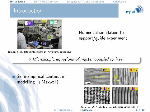
Introduction
fzu.cz/sites/default/�les/images/vyzkum/hilase.jpg
Numerical simulation tosupport/guide experiment
⇒ Microscopic equations of matter coupled to laser
Semi-empirical continuummodelling (+Maxwell)
Quantum mechanicaldescription (+photons)
Cong et al., Opt. Express 23, 5357-5367 (2015)M.Ruggenthaler FluidQED 1 / 10

Introduction DFTs for paramters Bridging DFTs and continuum Conclusion
Introduction
fzu.cz/sites/default/�les/images/vyzkum/hilase.jpg
Numerical simulation tosupport/guide experiment
⇒ Microscopic equations of matter coupled to laser
Semi-empirical continuummodelling (+Maxwell)
Quantum mechanicaldescription (+photons)
Cong et al., Opt. Express 23, 5357-5367 (2015)M.Ruggenthaler FluidQED 1 / 10

Introduction DFTs for paramters Bridging DFTs and continuum Conclusion
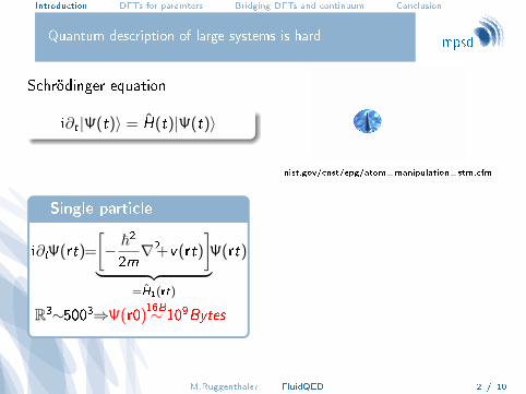
Quantum description of large systems is hard
Schrödinger equation
i∂t |Ψ(t)〉 = H(t)|Ψ(t)〉
nist.gov/cnst/epg/atom−manipulation−stm.cfm
M.Ruggenthaler FluidQED 2 / 10

Introduction DFTs for paramters Bridging DFTs and continuum Conclusion
Quantum description of large systems is hard
Schrödinger equation
i∂t |Ψ(t)〉 = H(t)|Ψ(t)〉
nist.gov/cnst/epg/atom−manipulation−stm.cfm
M.Ruggenthaler FluidQED 2 / 10

Introduction DFTs for paramters Bridging DFTs and continuum Conclusion
Quantum description of large systems is hard
Schrödinger equation
i∂t |Ψ(t)〉 = H(t)|Ψ(t)〉
nist.gov/cnst/epg/atom−manipulation−stm.cfm
M.Ruggenthaler FluidQED 2 / 10
Introduction DFTs for paramters Bridging DFTs and continuum Conclusion
Quantum description of large systems is hard
Schrödinger equation
i∂t |Ψ(t)〉 = H(t)|Ψ(t)〉
nist.gov/cnst/epg/atom−manipulation−stm.cfm
Single particle
i∂tΨ(rt)=
[− ~2
2m∇2+v(rt)
]︸ ︷︷ ︸
=H1(rt)
Ψ(rt)
R3∼5003⇒Ψ(r0)16B∼ 109Bytes
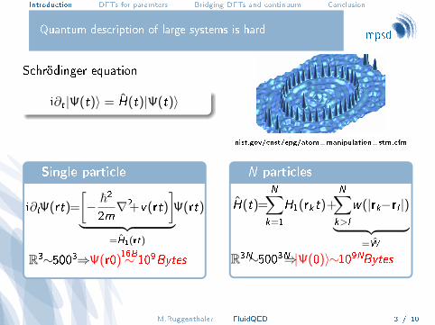
N particles
H(t)=N∑
k=1
H1(rkt)+N∑k>l
w(|rk−rl |)︸ ︷︷ ︸=W
R3N∼5003N⇒|Ψ(0)〉∼109NBytes
N = 2 leads to one exabyte (google-mail storage capacity of 2012)
M.Ruggenthaler FluidQED 3 / 10

Introduction DFTs for paramters Bridging DFTs and continuum Conclusion
Quantum description of large systems is hard
Schrödinger equation
i∂t |Ψ(t)〉 = H(t)|Ψ(t)〉
nist.gov/cnst/epg/atom−manipulation−stm.cfm
Single particle
i∂tΨ(rt)=
[− ~2
2m∇2+v(rt)
]︸ ︷︷ ︸
=H1(rt)
Ψ(rt)
R3∼5003⇒Ψ(r0)16B∼ 109Bytes
N particles
H(t)=N∑
k=1
H1(rkt)+N∑k>l
w(|rk−rl |)︸ ︷︷ ︸=W
R3N∼5003N⇒|Ψ(0)〉∼109NBytes
N = 2 leads to one exabyte (google-mail storage capacity of 2012)
M.Ruggenthaler FluidQED 3 / 10

Introduction DFTs for paramters Bridging DFTs and continuum Conclusion
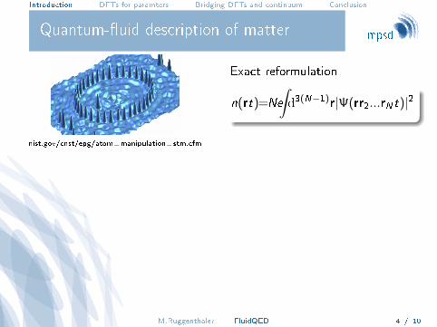
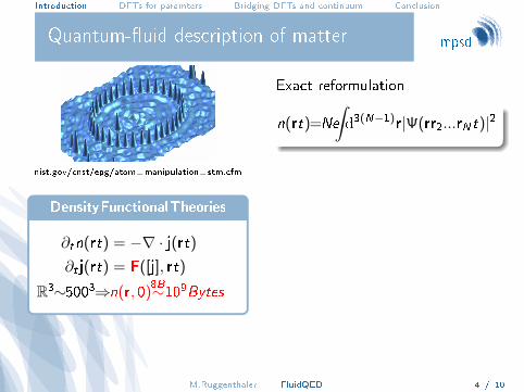
Quantum-�uid description of matter
nist.gov/cnst/epg/atom−manipulation−stm.cfm
Exact reformulation
n(rt)=Ne∫d3(N−1)r|Ψ(rr2...rNt)|2
DensityFunctionalTheories
∂tn(rt) = −∇ · j(rt)
∂t j(rt) = F([j], rt)
R3∼5003⇒n(r, 0)8B∼109Bytes
Kohn-Shamapproach
HKS(t) =N∑
k=1
HKS(rkt) + W
R3∼5003⇒|Φ(t)〉16B∼N×109Bytes
N ∼ 104 particles achievable for Kohn-Sham calculations
M.Ruggenthaler FluidQED 4 / 10
Introduction DFTs for paramters Bridging DFTs and continuum Conclusion
Quantum-�uid description of matter
nist.gov/cnst/epg/atom−manipulation−stm.cfm
Exact reformulation
n(rt)=Ne∫d3(N−1)r|Ψ(rr2...rNt)|2
DensityFunctionalTheories
∂tn(rt) = −∇ · j(rt)
∂t j(rt) = F([j], rt)
R3∼5003⇒n(r, 0)8B∼109Bytes
Kohn-Shamapproach
HKS(t) =N∑
k=1
HKS(rkt) + W
R3∼5003⇒|Φ(t)〉16B∼N×109Bytes
N ∼ 104 particles achievable for Kohn-Sham calculations
M.Ruggenthaler FluidQED 4 / 10
Introduction DFTs for paramters Bridging DFTs and continuum Conclusion
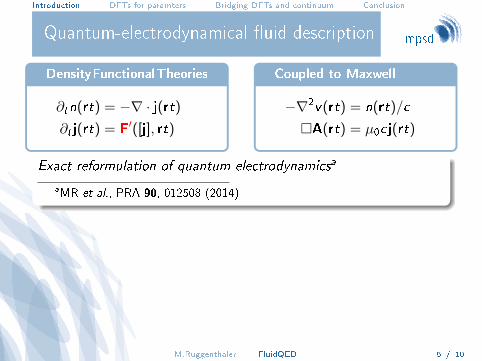
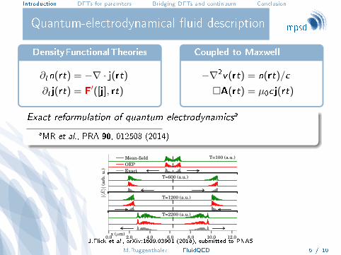
Quantum-electrodynamical �uid description
DensityFunctionalTheories
∂tn(rt) = −∇ · j(rt)
∂t j(rt) = F′([j], rt)
Coupled to Maxwell
−∇2v(rt) = n(rt)/c
�A(rt) = µ0cj(rt)
Exact reformulation of quantum electrodynamicsa
aMR et al., PRA 90, 012508 (2014)
T=100 (a.u.)Mean-fieldOEPExact
|〈E〉|
(arb
.u.)
T=600 (a.u.)
T=1200 (a.u.)
0.0 2.0 4.0 6.0 8.0 10.0 12.0
T=2200 (a.u.)
x (µm)J.Flick et al., arXiv:1609.03901 (2016), submitted to PNAS
M.Ruggenthaler FluidQED 5 / 10
Introduction DFTs for paramters Bridging DFTs and continuum Conclusion
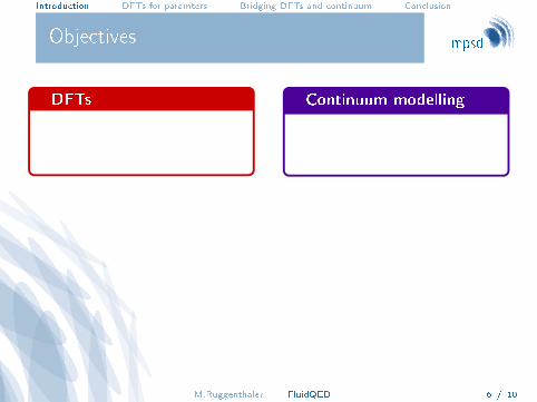
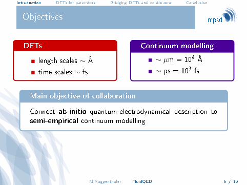
Objectives
DFTs
length scales ∼ Å
time scales ∼ fs
Continuum modelling
∼ µm = 104 Å
∼ ps = 103 fs
Main objective of collaboration
Connect ab-initio quantum-electrodynamical description tosemi-empirical continuum modelling
1 DFTs provide parameters for continuum modelling
2 Averaging DFT equations: towards novel continuum approach
M.Ruggenthaler FluidQED 6 / 10

Introduction DFTs for paramters Bridging DFTs and continuum Conclusion
Objectives
DFTs
length scales ∼ Å
time scales ∼ fs
Continuum modelling
∼ µm = 104 Å
∼ ps = 103 fs
Main objective of collaboration
Connect ab-initio quantum-electrodynamical description tosemi-empirical continuum modelling
1 DFTs provide parameters for continuum modelling
2 Averaging DFT equations: towards novel continuum approach
M.Ruggenthaler FluidQED 6 / 10
Introduction DFTs for paramters Bridging DFTs and continuum Conclusion
Parameters for continuum modelling
T.Derrien et al., in preparation
For instance
∆n(rt) = n(rt)− nGS(r)
slab of silicon irradiated by laser
Number of excited electrons (single color)
M.Ruggenthaler FluidQED 7 / 10

Introduction DFTs for paramters Bridging DFTs and continuum Conclusion
Parameters for continuum modelling
T.Derrien et al., in preparation
For instance
∆n(rt) = n(rt)− nGS(r)
slab of silicon irradiated by laser
Number of excited electrons (single color)
M.Ruggenthaler FluidQED 7 / 10

Introduction DFTs for paramters Bridging DFTs and continuum Conclusion
Parameters for continuum modelling
T.Derrien et al., in preparation
For instance
∆n(rt) = n(rt)− nGS(r)
slab of silicon irradiated by laser
Number of excited electrons (single color)
M.Ruggenthaler FluidQED 7 / 10
Introduction DFTs for paramters Bridging DFTs and continuum Conclusion
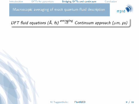
Macroscopic averaging of exact quantum-�uid description
DFT �uid equations (Å, fs)averaging⇒ Continuum approach (µm, ps)
T. J.-Y. Derrien1,2, N. Tancogne-Dejean2, M. Ruggenthaler2, H. Appel2, A. Rubio2,3,4, N. M. Bulgakova1,5
Bridging quantum mechanics and continuum modeling: Macroscopic averaging of exact quantum fluid description
CONCLUSIONS REFERENCES
INTRODUCTION
1HiLASE Centre, Institute of Physics ASCR, v.v.i, Dolní Brežany Czech Republic; 2Max Planck Institute for Structure and Dynamics of Matter, Hamburg, Germany;
3Physics Department, University of Hamburg, and the Hamburg Center for Ultrafast Imaging, Hamburg, Germany; 4Nano-Bio Spectroscopy Group and ETSF, Universidad del Pais Vasco, San Sebastian, Spain;
5Institute of Thermophysics SB RAS, Novosibirsk, Russia.
MACROSCOPIC AVERAGING2,3
Objectives: ♦
Context: ♦
♦
♦ Marie Skłodowska Curie Actions (MSCA) Individual Fellowship of the European’s Union’s (EU) Horizon 2020 Programme under grant agreement ”QuantumLaP” No. 657424.♦ ERC Advanced grant "DYNAMO" ♦ State budget of the Czech Republic (project HiLASE: Superlasers for the real world: LO1602).
CAN WE NEGLECT SOME OF THE FLUCTUATION TERMS?
FINANCIAL SUPPORTS:
♦ ♦ ♦ ♦
EXACT QUANTUM FLUID DESCRIPTION
Obtain an averaged form of the exact quantum fluid description of coupled light-matter systems, allowing for accurate and parameter-free large-scale modeling.
Continuum modeling is a powerful and accurate semi-empirical approach for modeling nanostructures and large-scale systems. However, it extensions to new phenomena is not straighfirward and requieres inputs from the experiement or other theoryQuantum mechanics is an exact theory but limited to small-size systems
Idea: Microscopic fluctuations of physical quantities are usually not important from the macroscopic perspective.
Method: Every function can be expressed as the sum of a macroscopic, or averaged part, and a microscopic, or fluctuating part
Importantly, the macroscopic averaging of the product of two functions is given by
which still contains the microscopic fluctuations of the two functions.
Quantum description of matter is usually described by a Schrodinger equation
which can be reformulated in terms of a exact coupled fluid equations of the form1
Pros: These are exact equations, allowing for a parameter-free description of any pertubation. Cons: Cannot be solved in practice for real systems.
,with of the form
MACROSCOPIC QUANTUM FLUID EQUATIONS
Applying the averaging procedure to the continuity equation Eq. (1) gives directly
The macroscopic averaging of Eq. (2) is more problematic as it leads to many terms, some of them including fluctuations.
Using of the fact that the potential is describing the electron-nuclei potential ( ) and the driving laser-field, we obtain the exact equation of motion for the total current
Fluctuation terms
Lorentz force
In order to understand if we can neglect some of the fluctuation terms, we consider the ideal situation of a perfect crystal ( ), under a uniform laser.In this case, the equation of motion of the current reduces to
We obtain that some of the fluctuation terms are negligible, whereas some of them leads to important physical effects.
One obtains also that neglecting the fluctuation terms here is equivalent to assuming a jellium model, i.e., .
Importantly, most of the fluctuation terms can be neglected in some ideal caseswhereas some of them are vital for describing correctly the physics.
Number of electron in the averaging volume
Responsible for HHG in perfect bulk materials4
We derived an exact quantum fluid description of coupled light-matter systemsMacroscopic fluid equations contain microscopic fluctuations.Some fluctuation terms can be neglected, but some of them lead to important physical effects.New framework to analyse approximation in continuum modeling
[1] R. van Leeuwen, Mapping from Densities to Potentials in Time-Dependent Density-Functional Theory. Phys. Rev. Lett. 82, 3863 (1999).[2]W. L. Mochán and R. G. Barrera, Electromagnetic response of systems with spatial fluctuations. I. General formalism.Phys. Rev. B 32, 4984 (1985).[3]R. Del Sole and E. Fiorino, Macroscopic dielectric tensor at crystal surfaces. Phys. Rev. B 29, 4631 (1984).[4]N. Tancogne-Dejean et al., Impact of the electronic band structure in high-harmonic generation spectra of solids. Submitted.
Details see poster of Nicolas
M.Ruggenthaler FluidQED 8 / 10

Introduction DFTs for paramters Bridging DFTs and continuum Conclusion
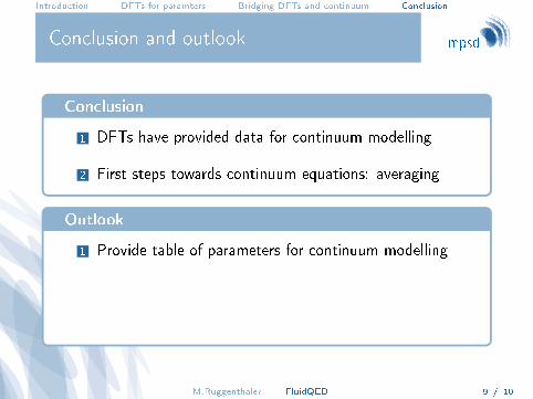
Conclusion and outlook
Conclusion
1 DFTs have provided data for continuum modelling
2 First steps towards continuum equations: averaging
Outlook
1 Provide table of parameters for continuum modelling
2 Light-matter propagation in solids
3 First-principles derivation of continuum modelling
M.Ruggenthaler FluidQED 9 / 10

Introduction DFTs for paramters Bridging DFTs and continuum Conclusion
Conclusion and outlook
Conclusion
1 DFTs have provided data for continuum modelling
2 First steps towards continuum equations: averaging
Outlook
1 Provide table of parameters for continuum modelling
2 Light-matter propagation in solids
3 First-principles derivation of continuum modelling
M.Ruggenthaler FluidQED 9 / 10

Introduction DFTs for paramters Bridging DFTs and continuum Conclusion
Thank you for your attention!
We acknowledge �nancial support from Marie Skªodowska Curie Actions (MSCA) Individual Fellowship
of the European's Union's (EU) Horizon 2020 Programme under grant agreement �QuantumLaP� No.
657424, European Research Council Advanced Grant "DYNAMO", State budget of the Czech Republic
(project HiLASE: Superlasers for the real world: LO1602).
M.Ruggenthaler FluidQED 10 / 10