Quantum Dot Charge–Sensor Physics in 2DEG Heterostructures

Morten KjærgaardSpring 2010

Abstract

In this paper I introduce and discuss the details of the theory and numerical programs de-veloped to understand the physics of a gate–defined quantum dot as a charge sensor for thecharge state of a nearby double quantum dot on 2DEG heterostructures.

This paper is intended as extended material and background for the paper

Fast sensing of double-dot charge arrangement and spin state with an rf sensor quantum dotC. Barthel, MK, J. Medford, M. Stopa, C. M. Marcus, M. P. Hanson, A. C. Gossard

Physical Review B: Rapid Communications, 81, 161308 (2010).

Contents

1 QuantumDots for Quantum Computation 3

2 Spin–qubit readout 32.1 Measuring Charge–State: Coulomb Blockade . . . . . . . . . . . . . . . . . . . . . . 32.2 Measuring the Spin–State: Pauli Blockade . . . . . . . . . . . . . . . . . . . . . . . . 4

3 Increasing the Charge–Sensitivity 5

4 Sensitivity and Lever–arms of Charge–sensors 7

5 Numerically Calculating the Sensitivity 75.1 SETE – self-consistent DFT for φ(x, y, z) and ρ(x, y, z) . . . . . . . . . . . . . . . . . . 85.2 gvQPCc – QPC Conductance . . . . . . . . . . . . . . . . . . . . . . . . . . . . . . . . 95.3 ivr – SQD Conductance . . . . . . . . . . . . . . . . . . . . . . . . . . . . . . . . . . 10

6 Conclusion & Outlook 12

List of Figures

1 Schematic of double quantum dots in 2–dimensional electron gases . . . . . . . . . 32 Cartoon depicting the process of charge–state readout of a quantum dot using a

proximal quantum point contact . . . . . . . . . . . . . . . . . . . . . . . . . . . . . 43 Charge–stability diagrams for a double quantum dot measured using adjacent

quantum point contact . . . . . . . . . . . . . . . . . . . . . . . . . . . . . . . . . . . 54 Schematic showing the principle behind a Pauli spin blockade. . . . . . . . . . . . . 55 SEM micrograph of geometry used for sensing quantum dot measurements in

Barthel et al. . . . . . . . . . . . . . . . . . . . . . . . . . . . . . . . . . . . . . . . . . 66 Charge–stability diagramsmeasured using a sensing quantum dot and a quantum

point contact in the geometry from figure 5. . . . . . . . . . . . . . . . . . . . . . . . 67 Self–consistently calculated electron density in the geometry used for sensing quan-

tum dot experiments . . . . . . . . . . . . . . . . . . . . . . . . . . . . . . . . . . . . 98 Self–consistently calculated potentials for use in the conductance calculation through

the QPC . . . . . . . . . . . . . . . . . . . . . . . . . . . . . . . . . . . . . . . . . . . 99 Examples of transverse 1D–potential from which eigenvalues for the effective lon-

gitudinal 1D–potential is created . . . . . . . . . . . . . . . . . . . . . . . . . . . . . 1010 Numerically calculated values of conductance through QPC for (0,2) and (1,1)

charge–states on a proximal double quantum dot. . . . . . . . . . . . . . . . . . . . 1111 Sensing quantum dot conductance calculated using SETE and ivr for two fixed

charge–states (1,1) and (0,2). . . . . . . . . . . . . . . . . . . . . . . . . . . . . . . . . 12

2 SPIN–QUBIT READOUT

1 Quantum Dots for Quantum Computation

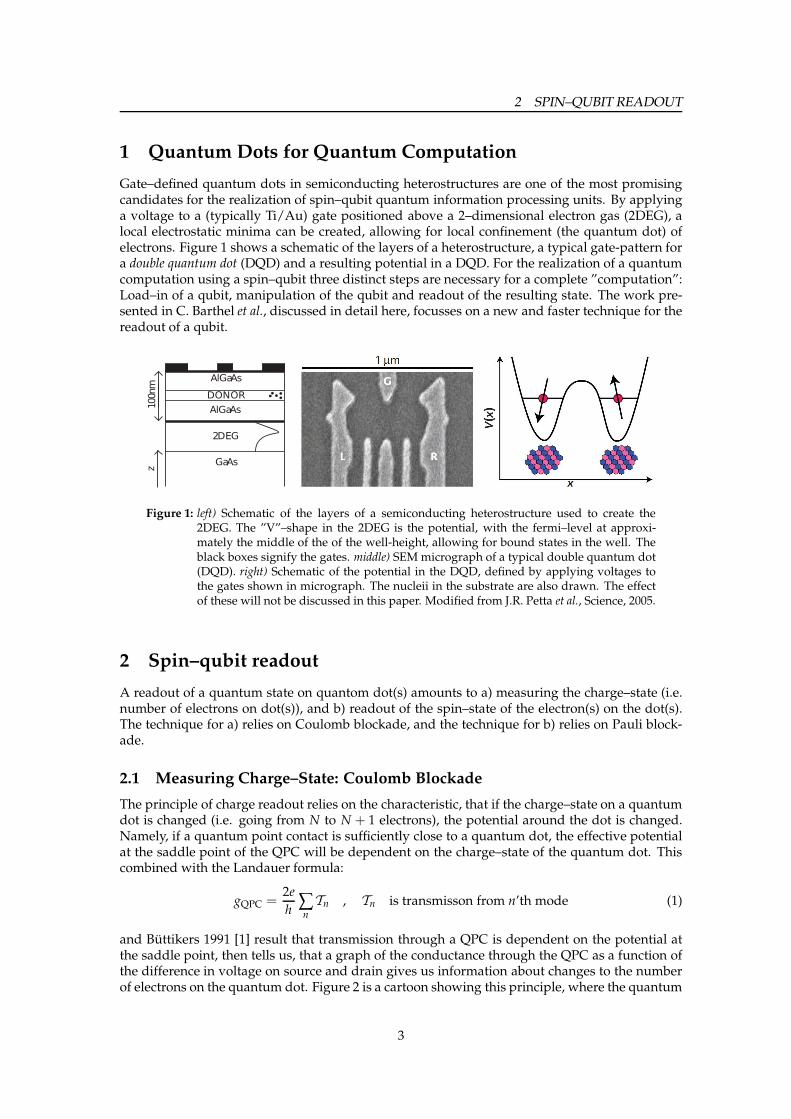
Gate–defined quantum dots in semiconducting heterostructures are one of the most promisingcandidates for the realization of spin–qubit quantum information processing units. By applyinga voltage to a (typically Ti/Au) gate positioned above a 2–dimensional electron gas (2DEG), alocal electrostatic minima can be created, allowing for local confinement (the quantum dot) ofelectrons. Figure 1 shows a schematic of the layers of a heterostructure, a typical gate-pattern fora double quantum dot (DQD) and a resulting potential in a DQD. For the realization of a quantumcomputation using a spin–qubit three distinct steps are necessary for a complete ”computation”:Load–in of a qubit, manipulation of the qubit and readout of the resulting state. The work pre-sented in C. Barthel et al., discussed in detail here, focusses on a new and faster technique for thereadout of a qubit.

Figure 1: left) Schematic of the layers of a semiconducting heterostructure used to create the2DEG. The ”V”–shape in the 2DEG is the potential, with the fermi–level at approxi-mately the middle of the of the well-height, allowing for bound states in the well. Theblack boxes signify the gates. middle) SEMmicrograph of a typical double quantum dot(DQD). right) Schematic of the potential in the DQD, defined by applying voltages tothe gates shown in micrograph. The nucleii in the substrate are also drawn. The effectof these will not be discussed in this paper. Modified from J.R. Petta et al., Science, 2005.

2 Spin–qubit readout

A readout of a quantum state on quantom dot(s) amounts to a) measuring the charge–state (i.e.number of electrons on dot(s)), and b) readout of the spin–state of the electron(s) on the dot(s).The technique for a) relies on Coulomb blockade, and the technique for b) relies on Pauli block-ade.

2.1 Measuring Charge–State: Coulomb Blockade

The principle of charge readout relies on the characteristic, that if the charge–state on a quantumdot is changed (i.e. going from N to N + 1 electrons), the potential around the dot is changed.Namely, if a quantum point contact is sufficiently close to a quantum dot, the effective potentialat the saddle point of the QPC will be dependent on the charge–state of the quantum dot. Thiscombined with the Landauer formula:

gQPC =2e

h ∑n

Tn , Tn is transmisson from n’th mode (1)

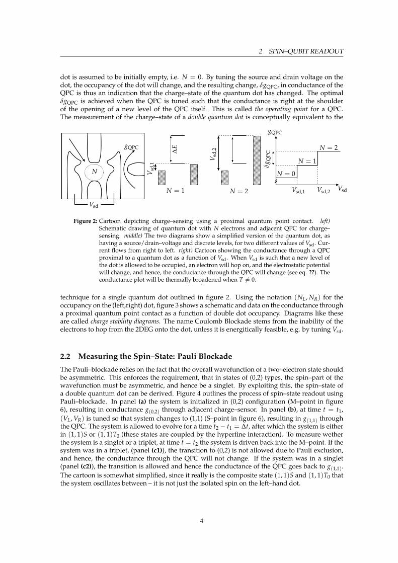
and Buttikers 1991 [1] result that transmission through a QPC is dependent on the potential atthe saddle point, then tells us, that a graph of the conductance through the QPC as a function ofthe difference in voltage on source and drain gives us information about changes to the numberof electrons on the quantum dot. Figure 2 is a cartoon showing this principle, where the quantum

3

2 SPIN–QUBIT READOUT

dot is assumed to be initially empty, i.e. N = 0. By tuning the source and drain voltage on thedot, the occupancy of the dot will change, and the resulting change, δgQPC, in conductance of theQPC is thus an indication that the charge–state of the quantum dot has changed. The optimalδgQPC is achieved when the QPC is tuned such that the conductance is right at the shoulderof the opening of a new level of the QPC itself. This is called the operating point for a QPC.The measurement of the charge–state of a double quantum dot is conceptually equivalent to the

Vsd,1

Vsd

,1

Vsd,2

Vsd

,2

gQPC

δgQPC

Vsd

Vsd

N = 1

N = 1

N = 2

N = 2

N = 0∆E

N

gQPC

Figure 2: Cartoon depicting charge–sensing using a proximal quantum point contact. left)Schematic drawing of quantum dot with N electrons and adjacent QPC for charge–sensing. middle) The two diagrams show a simplified version of the quantum dot, ashaving a source/drain–voltage and discrete levels, for two different values of Vsd. Cur-rent flows from right to left. right) Cartoon showing the conductance through a QPCproximal to a quantum dot as a function of Vsd. When Vsd is such that a new level ofthe dot is allowed to be occupied, an electron will hop on, and the electrostatic potentialwill change, and hence, the conductance through the QPC will change (see eq. ??). Theconductance plot will be thermally broadened when T 6= 0.

.

technique for a single quantum dot outlined in figure 2. Using the notation (NL,NR) for theoccupancy on the (left,right) dot, figure 3 shows a schematic and data on the conductance througha proximal quantum point contact as a function of double dot occupancy. Diagrams like theseare called charge stability diagrams. The name Coulomb Blockade stems from the inability of theelectrons to hop from the 2DEG onto the dot, unless it is energitically feasible, e.g. by tuning Vsd.

2.2 Measuring the Spin–State: Pauli Blockade

The Pauli–blockade relies on the fact that the overall wavefunction of a two–electron state shouldbe asymmetric. This enforces the requirement, that in states of (0,2) types, the spin–part of thewavefunction must be asymmetric, and hence be a singlet. By exploiting this, the spin–state ofa double quantum dot can be derived. Figure 4 outlines the process of spin–state readout usingPauli–blockade. In panel (a) the system is initialized in (0,2) configuration (M–point in figure6), resulting in conductance g(0,2) through adjacent charge–sensor. In panel (b), at time t = t1,

(VL,VR) is tuned so that system changes to (1,1) (S–point in figure 6), resulting in g(1,1) throughthe QPC. The system is allowed to evolve for a time t2 − t1 = ∆t, after which the system is eitherin (1, 1)S or (1, 1)T0 (these states are coupled by the hyperfine interaction). To measure wetherthe system is a singlet or a triplet, at time t = t2 the system is driven back into the M–point. If thesystem was in a triplet, (panel (c1)), the transition to (0,2) is not allowed due to Pauli exclusion,and hence, the conductance through the QPC will not change. If the system was in a singlet(panel (c2)), the transition is allowed and hence the conductance of the QPC goes back to g(1,1).

The cartoon is somewhat simplified, since it really is the composite state (1, 1)S and (1, 1)T0 thatthe system oscillates between – it is not just the isolated spin on the left–hand dot.

4

3 INCREASING THE CHARGE–SENSITIVITY

Figure 3: Coupled double–dot generalization of charge–sensing using adjacent quantum pointcontact. left) Schematic showing (left,right)–occupancy of the double–dot as a functionof VL ∼ Vg1 and VR ∼ Vg2. Current only flows through the system at the triple-points,denoted by black circles. Adapted from A.C. Johnsons PhD Thesis, 2005. right) Datafrom device in figure 1 with indication of the double–dot occupancy, identified by es-tablishing the (0,0)–occupancy, and tuning VL and VR whilst looking for δgQPC. Adaptedfrom J.R. Petta et al, Science, 2005.

gSQD

t1

t1

t1

t1

t2

t2

t2

t2

t

t

t

t

g(0,2

)g(0,2

)

g(0,2

)g(0,2

)

g(1,1

)g(1,1

)

g(1,1

)g(1,1

)

(a)

(b)

(c1)

(c2)

t < t1

t = t1 t > t2

t > t2

Figure 4: Schematic showing principle behind Pauli blockade. See text for details. The blue spinwill only return to (0,2) configuration if the time spent in (1,1) (t2 − t1) is equal to twofull (or multiples thereof) spin flips. The step–like charicature of the conductance willbe thermally and tunneling broadened.

3 Increasing the Charge–Sensitivity

Charge–sensing in 2DEG heterostructure is thus of fundamental importance since it gives infor-mation about charge–occupancy, and even more important, about the spin–state. In the frame-work of quantum computing the knowledge of spin–state is equivalent to knowledge of the out-come of a quantum calculation (is the outcome a binary zero, e.g. a singlet, or is the outcomea binary 1, e.g. a triplet?). The work presented in Barthel et al. is a variant of the QPC chargereadout scheme that have so far been employed. The QPC is replaced with a quantum dot,termed the sensing quantum dot (SQD). The SQD is tuned such that it is right at the opening ofa new coulomb peak, and the conductance through the SQD is now measured as a function ofthe source and drain voltage on the quantum dot. Figure 5 shows a micrograph of the geometryof the system employed in the study in Barthel et al. along with the conductance through theQPC and SQD. In Barthel et al. we present charge–stability diagrams equivalent to the ones infigure 3 obtained using the SQD–technique. Figure 6 shows the charge–stability diagrams andthe increased value of δgSQD over δgQPC. Simply modeling the change of the double–dot occu-

5

3 INCREASING THE CHARGE–SENSITIVITY

1.0

0.8

0.6

0.4

0.2

0.0

g (

e2/ h) QPC1

QPC2 Dot-Sensor

Figure 5: left) SEMmicrograph of device similar to the one used for measurements in Barthel et al.The QPC formed at the left–hand side of the DQD is used for comparison with the SQDthroughout the rest of the discussion. right) Conductance through QPC1 (blue), QPC2(black), and the SQD (red) as a function of the respective backgates (VQ1, VQ2 and VD).The operating point for the SQD is at the shoulder of a coulomb peak.

pancy as changing the effective potential in the proximal SQD and QPC would already lead oneto the conclusion that δgSQD > δgQPC simply due to the difference in slope of conductance plotsin figure 5. It turns out that this, however, is not the complete story. This is due to the differenteffective lever–arms of the SQD and QPC. The effective lever–arm is the number that relates thechange in some back–gate voltage (or a change in double dot occupancy) to the actual change inthe electrostatic potential at the saddle point of the QPC / electrostatic potential at the center ofthe dot. Numerical simulations allow us to estimate this effective lever–arm, and the calculationof these, will be the subject of the next section.

(b)(a)

(0,1)

(1,1)

(0,2)(0,1)

(1,2)S

M

-0.5 0.50 1∆g g 0 0.02-0.02∆g g

(c) (d)

(0,2)

(1,1)(1,2)

0 2 4-2-4

0.30

0.20

0.10

0 2 4-2-4

0.306

0.304

0.302

0.300

Detuning (mV) Detuning (mV)

Figure 6: left) Charge–stability diagram of the double quantum dot measured using the sensingquantum dot in figure 5 tuned to the operating point. The line–cut below clearly showsthe difference δgSQD in conductance through SQD when tuning VL and VR to allow the(1, 1) ↔ (0, 2)–transition. right) Equivalent data obtained using the quantum point con-tact labeled QPC1 in figure 5. In both charge–stability diagrams the color–scale showsthe relative difference ∆g/g, where ∆g = g(1,1) − g(0,2) and g = (g(1,1) + g(0,2))/2

6

5 NUMERICALLY CALCULATING THE SENSITIVITY

4 Sensitivity and Lever–arms of Charge–sensors

In Barthel et al. we introduce a measure of the sensitivity, s, of a QPC or QD as follows:

sQPC =∂g

∂VQPC=

∂g

φSP

∂φSP

∂VQPC= αQPC

∂φSP

∂VQPC

sSQD =∂g

∂Vdot=

∂g

∂φdot

∂φdot

∂Vdot= αSQD

∂φdot

∂Vdot,

where V is the back–gate voltage on QPC or QD, and φ is the electrostatic potential at the saddlepoint (QPC) or middle of dot (QD). The number α is the effective leverarm, that depends on po-sition of nearby conductors that screen the interaction between the source of the voltage and thepotential at the point of interest. The issue of sensitivity of the QPC vs a SQD can now be quan-tified by establishing the numerical value of the leverarms. Using the three numerical methodsdescribed below, we find a ratio of αSQD/αQPC ∼ 20, arising from screening from conductors,as calculated using self–consistent density functional theory modeling of the geometry shown infigure 5.

5 Numerically Calculating the Sensitivity

The numerical values for the QPC are found as follows. Details of the SETE code in step 1 can befound in section 5.1 (and ref [2], and the details of the gvQPCc code in step 2–3 can be found insection 5.2.

1. Using self–consistent density functional theory (within the local density and effective massapproximation), Poissons equation is solved in the full 3D geometry from experiment (in-cluding gate–geometry, gate–voltages, depth of 2DEG etc). This yields and effective two–dimensional potential and density of the entire geometry. See figure 7

2. By cutting out the part of the 2D potential in the area around the QPC and solving thetransverse Schrodinger equation in slices through this area, an effective 1D potential for thelowest subband can be created.

3. Using a WKB approximation to the transmission through this effective 1D potential, thetransmission, and hence conductance (see eq. 1), can be found.

Equivalently, for the SQD, the numerical values are found as follows (for details on step 1, see5.1, for details on step 2 see 5.3).

1. Using the SETE code, the free energy, FSQD, as a function of the back–gate voltage and thenumber of electrons on the dot N is evaluated for the full 3D geometry.

2. The conductance through the SQD is calculated using Beenakkers 1991 result [3], in thelow–tunneling regime, with FSQD(VSQD,N) as input.

The simulations produced for the Barthel et al. paper were generated using three different pro-grams. Two are developed by Mike Stopa, SETE [2], for calculating the potential and charge–density of a gate-defined 2DEG heterostructure, and ivr [4], for evaluating the conductancethrough a quantum dot, using Beenakkers conductance formula [3]. The code gvQPCc is de-veloped by MK, and uses a WKB approximation to the potential in a quantum point contact toevaluate the conductance.

7

5 NUMERICALLY CALCULATING THE SENSITIVITY

5.1 SETE – self-consistent DFT for φ(x, y, z) and ρ(x, y, z)

SETE, Single Electron Tunneling Elements, is a self–consistent code for calculating the electronicstructure of semiconductor quantum dots. The code uses density functional theory (within theeffective mass and local density approximations) to solve the 3D Poisson equation

−∇2φ(x, y, z) =4πǫ

κρ(x, y, z) (2)

and calculate the free energy, F , of quantum dot systems. In the paper SETE is used to find a) theeffective 2D-potential of a quantum point contact at the depth of the 2 dimensional electron gas inan AlxGa1−xAs-GaAs heterostructure and b) the free energy of a quantum dot, both of which arelocated adjacent to a laterally defined double quantum dot. The result of a) is used in gvQPCc andthe result of b) is used in ivr.

SETE fully incorporates gate-geometry, donor concentration, depth of 2DEG and voltages ongates. After initializing the entire device, an inhomogeneous grid is set up on the gate-geometry,and the density is found at each lattice-site using either a quantum mechanical solution (in thequantum dots, or regions of interest) or a classical solution (in regions of less importance).

For the quantum mechanical solution, we are in principle looking for solutions to the full 3D-Schrodinger equation

[

−h2

2m∗∇2 + eφ(x, y, z) + VB(z)

]

ψ(x, y, z) = Eψ(x, y, z), (3)

where VB(z) is the band offset between the AlGaAs and the GaAs at the interface, and m∗ is theeffective mass, m∗ ≈ 0.067m. Equation (3) is intractable, and instead, an adiabatic approximationis assumed to reduce the 3D-potential to an effective 2D-potential. A 1D-Schrodinger equation issolved at each lattice site

[

−h2

2m∗∂2z + eφxy(z) + VB(z)

]

ξxyn (z) = ǫ

xyn ξ

xyn (z), (4)

where superscript x, y denotes discrete indices on the lattice. z–direction is the growth-directionof the sample. The discrete 2D-potential is now interpreted as the continuous effective poten-tial ǫ0(x, y), where we assume only filling of the lowest subband. Assuming adiabadicity, i.e.∂xξxy(z) = ∂yξxy(z) = 0, the 3D-density in the poisson equation can now be found by solving a2D-Schrodinger

[

−h2

2m∗

(

∂2x + ∂2y

)

+ ǫ0(x, y)

]

f0(x, y) = E f0(x, y), (5)

from which the density is calculated as

ρQM(x, y, z) = e|ψ(x, y, z)|2 = e| f0(x, y)ξxy(z)|2. (6)

The density is calculated ”classically” in regions far from the quantum dot(s), using the Thomas-Fermi approximation, i.e. we assume the potential varies slowly on scale of 1/λF. Under thisassumption the density is found from

ρcl(x, y, z) =ǫ0(x, y)− µ

2π|ξxy(z)|2,

so we do not need to find the full eigenstates, as in eq. 6

The classical and quantummechanical densities are patched together to update the poisson equa-tion, which is solved again, using the Bank-Rose method [5], to yield a new 3D-potential, and theprocedure is iterated until convergence. We apply Dirichlet boundary conditions at lattice–pointsin the gates, i.e. φ(x, y, z) = Vg , and Neumann boundary conditions elsewhere, ∇φ(x, y, z) = 0.A sample density, calculated with SETE is depicted in fig. 7

8

5 NUMERICALLY CALCULATING THE SENSITIVITY

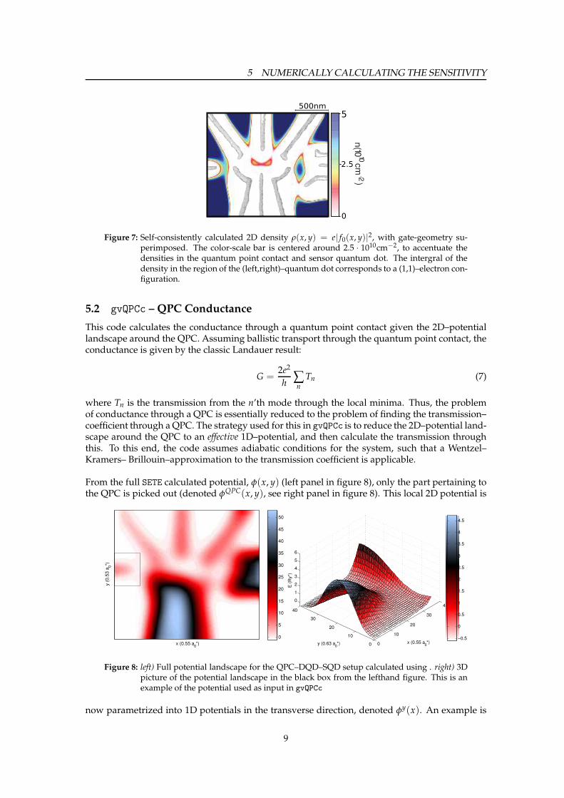
Figure 7: Self-consistently calculated 2D density ρ(x, y) = e| f0(x, y)|2, with gate-geometry su-

perimposed. The color-scale bar is centered around 2.5 · 1010cm−2, to accentuate thedensities in the quantum point contact and sensor quantum dot. The intergral of thedensity in the region of the (left,right)–quantum dot corresponds to a (1,1)–electron con-figuration.

5.2 gvQPCc – QPC Conductance

This code calculates the conductance through a quantum point contact given the 2D–potentiallandscape around the QPC. Assuming ballistic transport through the quantum point contact, theconductance is given by the classic Landauer result:

G =2e2

h ∑n

Tn (7)

where Tn is the transmission from the n’th mode through the local minima. Thus, the problemof conductance through a QPC is essentially reduced to the problem of finding the transmission–coefficient through a QPC. The strategy used for this in gvQPCc is to reduce the 2D–potential land-scape around the QPC to an effective 1D–potential, and then calculate the transmission throughthis. To this end, the code assumes adiabatic conditions for the system, such that a Wentzel–Kramers– Brillouin–approximation to the transmission coefficient is applicable.

From the full SETE calculated potential, φ(x, y) (left panel in figure 8), only the part pertaining tothe QPC is picked out (denoted φQPC(x, y), see right panel in figure 8). This local 2D potential is

x (0.55 a0*)

y (

0.5

3 a

0*)

0

5

10

15

20

25

30

35

40

45

50

Figure 8: left) Full potential landscape for the QPC–DQD–SQD setup calculated using . right) 3Dpicture of the potential landscape in the black box from the lefthand figure. This is anexample of the potential used as input in gvQPCc

now parametrized into 1D potentials in the transverse direction, denoted φy(x). An example is

9

5 NUMERICALLY CALCULATING THE SENSITIVITY

shown in the left panel of figure 9, which is exactly the 1D potential corresponding to y = 25 infigure 8. The Schrodinger equation for the lowest energy state in this potential reads

Hy=25(x)ψy=250 (x) = ǫ

y=250 ψ

y=250 (x). (8)

This equation is solved numerically to find ǫy=250 . By looping over all 1D linecuts, φyi(x) in

φQPC(x, y) and solving equation 8, an ensemble of eigenvalues, {ǫyi0 } is found for a given gate–

voltage configuration on the entire geometry. The code then assumes a continuous limit of

potential–cuts, such that {ǫyi0 } → ǫ0(y). A plot of a sample ǫ0(y) calculated from φQPC(x, y)

is shown on the right panel of figure 9. The black circled eigenvalue is ǫy=250 , and Fermi–energy

at E = 0. Finally, the transmission is found through the effective 1D potential given by ǫ0(y)

0 5 10 15 20 25 30 35 400

0.5

1

1.5

2

2.5

3

3.5

4

x (0.55 a0*)

E / R

y*

0 5 10 15 20 25 30 35 40−0.6

−0.5

−0.4

−0.3

−0.2

−0.1

0

0.1

y (0.63a0*)

E (

Ry*)

Figure 9: left)An example of a 1D–linecut at y = 25 in the 3D plot fromfigure 8, denoted φy=25(x).This is the potential for which the lowest eigenstate is found in eq. (8). right) This graphshows the result of looping over all values of y in the 3D potential in figure 8, findingthe lowest eigenvalues, and plotting them as function of y, denoted ǫ0(y). This is thepotential fromwhich the transmission usingWKB is calculated. The marked eigenvalueis the lowest eigenvalue from the potential on the left.

using a WKB approximation,

TWKB0 = exp

[

2∫

dy√

2m(ǫ0(y)− µ)

]

(9)

which is plugged into the Landauer equation, assuming transmission only from the lowest–lyingstate:

G(VQPC) =2e2

hTWKB0 (VQPC). (10)

In the paper we performed this calculation for values of gate–voltages corresponding to the mea-sured values in the experiment. By numerically fixing the charge–density in the double quan-tum dot to (0,2) and (1,1), and looping over gate–voltages, we were able to quantify the differ-ence in conductance due to charge–rearrangement, as plotted in figure 10. For the QPC we find|∆g|/g ∼ 0.1, roughly consistent with the experimental value (0.03). The difference is primarilyattributed to breakdown of the breakdown of WKB approximation close to the classical turningpoint.

5.3 ivr – SQD Conductance

This code calculates the conductance through a quantum dot using Beenakkers 1991 result [3].Using a master equation approach, a linear-response theory calculation of the transport through

10

5 NUMERICALLY CALCULATING THE SENSITIVITY

1.0

g (

e2

/h)

-30 -20 -10 0∆V

Q1(mV)

0.04

0.00|∆

g| (e

2/h)0.0

g(0,2)

g(1,1)

∆g

(b)

Figure 10: The conductance through a proximal quantum point contact as function of back–gatevoltage. The conductance is numerically calculated for two different, but fixed, charge–densities on a proximal double quantum dot. The black line is the relative difference.Consistent with experiment the relative difference in conductance is largest at the op-erating point.

a quantum dot yields the equation

G(Vg) =e2

kBT∑{ni}

Peq({ni}) ∑p

δnp,0γp f (F ({ni + p},N + 1,Vg) −F ({ni},N,Vg)− µ), (11)

the first sum is on electron-configurations on the dot, and the second sum is over levels on thedot. Peq is the Gibbs distribution for the configuration

Peq({ni}) =exp(−βF ({ni},N,Vg) − µ)

∑{ni}exp(−βF ({ni},N,Vg) − µ)

. (12)

The δ-function ensures that the on-dot level is empty, and γp is the tunneling coupling of levelp, which is simply set to 1 for all p. f is the fermi-function, µ is the chemical potential of thesource–drain, F is the free energy of the dot for a given electron configuration, {ni}, the totalnumber of electrons, and the voltage of the plunger-gate. We truncate the summation in the par-tition function in the denominator of eq.(12), by only taking into account contributions from theoccupation–numbers Nmin1 and Nmin2 which minimizes the free energy. In the constant interac-tion approximation, for example, the free energy of a quantum dot is given by

F =(eN)2

2CQD-gate+ eNαVg,

which is a parabola in N, so terms far from Nmin1 and Nmin2 will not contribute significantly.Thus, truncating the sum yields the Gibbs distribution used in ivr

Peq({ni}N) =exp(−βF ({ni},N,Vg) − µ)

exp(−βF ({ni},Nmin1,Vg) − µ) + exp(−βF ({ni},Nmin2,Vg)− µ)(13)

The ivr code takes as input the gate–voltage, the on dot electron number and the associated freeenergy, which is calculated by SETE, for Nmin1 and Nmin2. The sums are then evaluated to yieldthe corresponding conductance. A conductance calculated using ivr can be seen in figure ??. Asin the case of the QPC, we have calculated the conductance keeping the charge–distribution onthe double quantum dot fixed at either (0,2) or (1,1). For the SQD we get an approximal valueof ∆g/g ∼ 1.4, also comparable to experiment (0.9). The primary cause of the discrepancy is theassumption that hγ ≪ kBT, where we experimentally find hγ ∼ kBT.

11

REFERENCES

g (

e /h)

2

(a)g

(0,2)g

(1,1)

Δg

D

0.0

0.5

-0.4

-0.2

0.2

0.4

0.0

0.0-0.5-1.0-1.5-2.0-2.5-3.0

Δg (e

/h)

2

VΔ (mV)

Figure 11: Sensing quantum dot conductance calculated using SETE and ivr for two fixed charge–states (1,1) and (0,2)

6 Conclusion

In this paper the concept of charge–sensing using an adjacent quantum point contact and an ad-jacent quantum dot was introduced. The theory of Coulomb blockade for charge–measurementsof quantum dots, and Pauli blockade for measurement of singlet/triplet states of double quan-tum dots were introduced. In the paper by Barthel et al. we used a quantum dot for sensing thecharge–state of a double quantum dot, which resulted in a factor of 30 increase in sensitivity. Byself–consistently modelling the device, we showed that this difference is primarily due to screen-ing effects from the 2DEG in the QPC as opposed to the isolated sensing quantum dot. Usingthe Pauli–blockade, we also show in Barthel et al. that the SQD allows for almost an order ofmagnitude reduction in the time needed for a singleshot spin–state readout.

References

[1] M. Buttiker. Quantized transmission of a saddle-point constriction. Phys. Rev. B, 41(11):7906–7909, Apr 1990.

[2] M. Stopa. Quantum dot self-consistent electronic structure and the coulomb blockade. Phys-ical Review B, 54(19):13767–13783, November 1996.

[3] C. W. J. Beenakker. Theory of coulomb-blockade oscillations in the conductance of a quantumdot. Physical Review B, 44(4):1646–1656, July 1991.

[4] M. Stopa. Coulomb oscillation amplitudes and semiconductor quantum-dot self-consistentlevel structure. Phys. Rev. B, 48(24):18340–18343,Dec 1993.

[5] R. E. Bank and D. J. Rose. Global approximate newton methods. Numerische Mathematik,37(2):279–295, 1981.

12