Quantum computing and entanglement formathematicians

Nolan R. Wallach

April 22, 2013

These notes are an expanded form of lectures to presented at the C.I.M.E.summer school in representation theory in Venice, June 2004. The sections ofthis article roughly follow the five lectures given. The first three lectures (sec-tions) are meant to give an introduction to an audience of mathematicians (ormathematics graduate students) to quantum computing. No attempt is givento describe an implementation of a quantum computer (it is still not absolutelyclear that any exist). There are also some simplifying assumptions that havebeen made in these lectures. The short introduction to quantum mechanics inthe first section involves an interpretation of measurement that is still being de-bated which involves the “collapse of the wave function”after a measurement.This interpretation is not absolutely necessary but it simplifies the discussion ofquantum error correction. The next two sections give an introduction to quan-tum algorithms and error correction through examples including fairly completeexplanations of Grover’s (unordered search) and Shor’s (period search and fac-torization) algorithms and the quantum perfect (five qubit) code. The last twosections present applications of representation and Lie theory to the subject.We have emphasized the applications to entanglement since this is the mostmathematical part of recent research in the field and this is also the main areato which the author has made contributions. The material in subsections 5.1and 5.3 appears in this article for the first time.

1 The basics

In his seminal paper [F1] Richard Feynman introduced the idea of a computerbased on quantum mechanics. Of course, all modern digital computers in-volve transistors that are by their very nature quantum mechanical. However,the quantum mechanics only plays a role in the theory that explains why thetransistor switches. The actual switch in the computer is treated as if it weremechanical. In other words as if it were governed by classical mechanics. Feyn-man had something else in mind. The basic operations of a quantum computerwould involve the allowable transformations of quantum mechanics, that is, uni-tary operators and measurements. The analogue of bit strings for a quantum

1

computer are superpositions of bit strings (we will make this precise later) andthe analogue of a computational step (for example the operation not on one bit)is a unitary operator on the Hilbert space of bit strings (say of a fixed length).The reason that Feynman thought that there was a need for such a “computer”is that quantum mechanical phenomena are extremely diffi cult (if not impos-sible) to model on a digital computer. The reason why the field of quantumcomputing has blossomed into one of the most active parts of the sciences is thework of Peter Shor [S1] that showed that on a (hypothetical) quantum computerthere are polynomial time algorithms for factorization and discrete logarithms.Since most of the security of the internet is based on the assumption that thesetwo problems are computationally hard (that is, the only known algorithms aresuperpolynomial in complexity) this work has attracted an immense amount ofattention and trepidation. In these lectures we will discuss a model for com-putation based on this idea and discuss its power, ways in which it differs fromstandard computation and its limitations. Before we can get started we needto give a crash course in quantum mechanics.

1.1 Basic quantum mechanics

The states of a quantum mechanical system are the unit vectors of a Hilbertspace, V , over C ignoring phase. In other words the states are the elementsof the projective space of all lines through the origin in V . If v, w ∈ V thenwe write 〈v|w〉 for the inner product of v with w. We will follow the physicsconvention so the form is conjugate linear in v and linear in w. Following Diraca vector gives rise to a “bra”, 〈v| and a “ket” |v〉 the latter is exactly the sameas v the former is the linear functional that takes the value 〈v|w〉 on w. Thus ifv is a state then 〈v|v〉 = 1. In these lectures most Hilbert spaces will be finitedimensional. For the moment we will assume that dimV < ∞. An observableis a self adjoint operator, A, on V . Thus A has a spectral decomposition

V =⊕λ∈R

Vλ

with A|Vλ = λI. We can write this as follows. The spaces Vλ are orthogonalrelative to the Hilbert space structure. Thus we can define the orthogonalprojection Pλ : V → Vλ. Then we have A =

∑λPλ. If v is a state then we set

vλ = Pλv. A measurement of the state v with respect to an observable A yieldsa number λ that is an eigenvalue of A with the probability ‖vλ‖2. This leads tothe following problem. If we do another measurement almost instantaneouslywe should get a value close to λ. Thus one would expect the probability to bevery close to 1 for the state to be in Vλ. In the standard formulation of quantummechanics this is “explained”by the collapse of the wave function. That is, ameasurement of by apparatus corresponding to the observable A has two effects.The first is an eigenvalue, λ of A (the measurement) with probability ‖vλ‖2 andthe second is that the state has collapsed to

vλ‖vλ‖

.

2

This is one of the least intuitive aspects of quantum mechanics. It has been thesubject of much philosophical discussion. We will not enter into this debateand will merely take this as an axiom for our system.If we have a quantum mechanical system then in addition to the Hilbert

space V we have a self adjoint operator H the Hamiltonian of the system. Theevolution of a state in this system is governed by Schroedinger’s equation

dφ

dt= iHφ.

Thus if we have the initial condition φ(0) = v then

φ(t) = eitHv.

Thus the basic dynamics is the operation of unitary operators. If U is a unitaryoperator on V then |Uv〉 = U |v〉 and 〈Uv| = 〈v|U−1. This is the only consistentway to have 〈Uv|Uv〉 = 〈v|v〉 for a unitary operator.

Of course, these finite dimensional Hilbert spaces do not exist in isolation.The state of the entire universe, u, is a state in a Hilbert space, U , governedby the Schroedinger equation with Hamiltonian HU . We we will simplify thesituation and think of the finite dimensional space V as a tensor factor of Uthat is

U = V⊗E

with E standing for the environment. This is not a tremendous assumptionsince in practice the part of the universe that will have a real effect on V is givenby this tensor product. Now, the Hamiltonian HU will not preserve the tensorproduct structure. Thus, even though we are attempting to do only operationson states in V the environment will cause the states to change in ways thatare beyond the control of the experiment that we might be attempting to doon states in V . Thus if we prepare a state on which we will do a quantummechanical operation, that is, by applying a unitary transformation or doing ameasurement we can only assume that the state will not “morph”into a quitedifferent state for a very short time. This uncontrolled change of the state iscalled decoherence caused by the environment.The fact that our small Hilbert space V is not completely isolated from the

rest of the universe is the reason why it is more natural to use density matricesas the basic states. A density matrix (operator) is a self adjoint operator T onV that is positive semi-definite and has trace 1. In this context a state v ∈ Vwould then be called a pure state and a density matrix a mixed state. If v isa pure state then its density matrix is |v〉 〈v|. We note that this operator isjust the projection onto the line corresponding to the pure state v. Thus wecan identify the pure states with the mixed states that have rank 1. If T is amixed state then T transforms under a unitary operator by T 7→ kTk−1 if k isunitary. If we have a pure state u in U then it naturally gives rise to a mixedstate on V which is called the reduced density matrix and is defined as follows.Let {ei} be an orthonormal basis of E. Then u =

∑vi⊗ei with vi ∈ V . The

3

reduced density matrix is∑|vi〉 〈vi|. More generally, if T is a mixed state on

U then it gives rise to a mixed state Tr2(T ) on V by the formula

〈w|Tr2(T )|v〉 =∑i

〈w⊗ei|T |v

⊗ei〉 .

This mixed state is the reduced density matrix. One checks easily that sinceunitary operators don’t necessarily preserve the tensor product structure thata unitary transformation of the state, T , will not necessarily entail a unitarytransformation of the reduced density matrix. We will mainly deal with purestates in these lectures. However, we should realize that this is a simplificationof what nature allows us to see.

1.2 Bits

Although it is not mandatory we will look upon digital computing as the ma-nipulation of bit strings. That is, we will only consider fixed sequences of 0’sand 1’s. One bit is either 0 or it is 1. Two bits can have one of four values00, 01, 10, 11. These four strings can be looked upon as the expansion in base 2 ofthe integers 0, 1, 2, 3, they can be looked upon as representatives of the integersmod 4, or they can be considered to be the standard basis of the vector spaceZ2 × Z2. In general, an n-bit computer can manipulate bit strings of length n.We will call n the word length of our computer. Most personal computers nowhave word length 32 (soon 64). We will not be getting into the subtleties ofcomputer science in these lectures. Also, we will not worry about the physicalcharacteristics of the machines that are needed to do bit manipulations. Acomputer also can hold a certain number of words in its memory. There arevarious forms of memory (fast, somewhat fast, less fast, slow) but we will ig-nore the differences. We will look upon a computer program as a sequence ofsteps (usually encoded by bit strings of length equal to the word length) whichimplement a certain set of rules that we will call the algorithm. The first stepinputs a bit string into memory. Each succeeding step operates on a sequenceof words in memory that came from the operation of the preceding step andproduces another sequence of words, which may or may not replace some of thewords from the previous step and may or may not put words into new memorylocations. If properly designed the program will have rules that terminate it andunder each of the rules an output of bit strings. That is the actual computation.There are, of course, other ways the program might terminate, for example itruns out of memory, it is terminated by the operating system for attemptingto access protected memory locations, or even that it is terminated by the userout of impatience. In these cases there is no (intended) output except possiblyan error message.This is the von Neumann model of computation. The key is that the com-

puter does one step of a program at a time. Most computers can actually doseveral steps at one time. But this is because the computers are actually sev-eral von Neumann computers working simultaneously. For example, a computermight have an adder and a multiplier that can work independently. Or it might

4

have several central processors that communicate with each other and attemptto do program steps simultaneously. These modifications will only lead to aparallelism that its determined by the number of processors and can only leadto a constant speed-up of a computation. For example if we have 10 von Neu-mann computers searching through a sequence of N elements with the task offinding one with a specified property. For example you have N−1 red chips and1 white one. The program might be set to divide the sequence into 10 subse-quences each of size N

10 and then each processor is assigned the job of searchingthrough through one part. In the worst case each processor will have to evaluateN10 elements. So we see a speed up of a factor of 10 over using one processorin this simple problem (slightly less since the worst case with one processor isN − 1).We will come back to a few more aspects of digital computing as we develop

a model for quantum computation.

1.3 Qubits

The simplest description of the basic objects to be manipulated by a quantumcomputer of word length n are complex superpositions of bit strings of lengthn. Since a bit string is a sequence of numbers and the coeffi cients of the super-positions can also be some of these numbers we will use the ket notation for thebit strings as pure states. These superpositions will be called qubits. Thus onequbit is a an element of the two dimensional vector space over C with states

a |0〉+ b |1〉

and |a|2 + |b|2 = 1. We will be dealing with qubits quantum mechanically sowe ignore phase (multiples by complex numbers of norm 1). Thus our space ofqubits is one dimensional projective space over C. We will think of this qubitas being in state |0〉 with probability |a|2 and in state |b|2. Although this is avast simplification we will take the simplest one step operation on a qubit to bea unitary operator (projective unitary operator to be precise).Contrasting this with bits we see that on the set of bits {0, 1} there are ex-

actly 2 basic reversible operations: the identity map and NOT that interchanges0 and 1. In the case of qubits we have a 3 dimensional continuum of basic oper-ations that can be done. There is only one caveat. After doing these operationswhich are diffi cult to impossible classically we must do a measurement to re-trieve a bit. This measurement will yield 0 or 1 with some probability. Thus ina very real sense going to qubits and allowing unitary transformations has nothelped at all.An element of 2 qubit space will be of the form

u = a |00〉+ b |01〉+ c |10〉+ d |11〉

with |a|2 + |b|2 + |c|2 + |d|2 = 1. We interpret this as u is in state |00〉 withprobability |a|2, in state |01〉 with probability |b|2, etc. Similarly for n qubits.The steps in a quantum computation will be unitary transformations. However,

5

each unitary transformation given in a step will have to be broken up into basictransformations that we can construct with a known and hopefully small cost(time and storage).A quantum program starts with an n qubit state, u0, the input, and then

does a sequence of unitary transformations Tj on the state so the steps areu1 = T1u0, ..., um = Tmum−1, and a rules for termination and at termination ameasurement. The output is the measurement and or the state to which themeasured state has collapsed.

References

[F1] R. P. Feynman, Simulating physics with computers, Int. J. Theor.Phys., 21(1982),

[S1] P. W. Shor, Algorithms for quantum computation, discrete logarithmsand factorizing, Proceedings 35th annual symposium on foundations of com-puter science, IEEE Press, 1994.

2 Quantum algorithms

In the last lecture we gave simple models for a classical and a quantum computa-tion. In this lecture we will give a very simple example of a quantum algorithmthat implements that does something that is impossible to do on a Von Neu-mann computer. We will next give a more sophisticated example of a quantumalgorithm (Grover’s algorithm [G1]) that does an unstructured search of N ob-jects of the type described in the last lecture in

√N steps. At the end of the

lecture we will introduce the quantum (fast) Fourier transform and explain whyon a (hypothetical) quantum computer it is exponentially faster than the FastFourier transform

2.1 Quantum parallelism

Suppose that we are studying a function, f , on bit strings that takes the values1 and −1 and assume that it takes only one step on a classical computer tocalculate its value given a bit string. For example the function that takesvalue 1 if the last bit is 0, −1 if it is 1. We will think of bit strings of lengthn as binary expansions of the numbers 0, 1, ..., 2n − 1. Thus our n qubit space,V , has the orthonormal basis |0〉 , |1〉 , ..., |N − 1〉 with N = 2n − 1. We canreplace f by the unitary operator defined by T |j〉 = f(j) |j〉. T operates on astate v ∈ V ,

v =N−1∑j=0

aj |j〉 ,N−1∑j=0

|aj |2 = 1

6

by

Tv =N−1∑j=0

f(j)aj |j〉 .

Quantum mechanically this means that we have calculated f(j) with the prob-ability |aj |2. In other words the calculation of T on this superposition seems tohave calculated all of the values of f(j) simultaneously if all of the |aj | > 0 inone quantum step. In a sense we have, but the rub is that if we do a measure-ment then all we have after a measurement is f(j) |j〉 with probability |aj |2 andsince we ignore phase the value the object we are calculating is lost. Perhaps itwould be better to decide that we will operate quantum mechanically and thenread of the coordinates classically? I assert that we will still not be able to makedirect use of this parallelism. The reason is that we are only interested in very

big N . In this situation the set of states,N−1∑j=0

aj |j〉, with |aj |2 all about the

same size have a complement in the sphere of extremely small volume. Thisimplies that most of the states will have probabilities, |aj |2 ∼ 1

N . If n is, say,1000 then all the coordinates will be too small to measure classically. We cansee this as follows. We consider the unit sphere in real N dimensional space.Let ωN be the O(N) invariant volume element on SN−1 that is normalized sothat ∫

SN−1ωN = 1.

We write a state in the form v = cos θu+ sin θ |N − 1〉 with −π2 ≤ θ ≤π2 . With

u an element of the unit sphere in N − 1 dimensional space. Then we have

ωN = cN cos θn−2ωN−1∧dθ

and cN ∼ C√N with C independent of N . The set of all v in the sphere with

last coordinate aN−1that satisfies |aN−1|2 ≥ r2 > 1N + ε with ε > 0 has volume

at most

C√N(1− r2)N2 −1 = C

√N(1− ε)N2 −1(1−

11−εN

)N2 −1

which is extremely small for N large.The upshot is that a quantum algorithm must contain a method of increasing

the size of the coeffi cient of the desired output so that when a measurement ismade will have the output with high probability.

2.2 The tensor product structure of n-qubit space

Recall that the standard (sometimes called the computational) basis of the spaceof 2 qubits is |00〉 , |01〉 , |10〉 , |11〉. A physicist would also write |0〉 |1〉 = |01〉.We mathematicians would rather think that the multiplication is a tensor prod-uct. That is |0〉 , |1〉 form the standard basis of C2. Then

|0〉⊗|0〉 , |0〉

⊗|1〉 , |1〉

⊗|0〉 , |1〉

⊗|1〉

7

form an orthonormal basis of C2⊗C2 with the tensor product Hilbert space

structure. In other words we identify |ab〉 with |a〉⊗|b〉. In this form the original

bit strings are fully decomposable that is are tensor products of n elements inC2. We will call an n-qubit state a product state if it is of the form

v1⊗v2⊗· · ·⊗vn

with ‖vi‖2 = 1 for i = 1, ..., n. One very important product state is the uniformstate (N = 2n):

v =1√N

N−1∑j=0

|j〉 .

To see that it is indeed a product state we set u = 1√2(|0〉 + |1〉). Then v =

u⊗· · ·⊗u (n-fold tensor product). This formula also shows that the uniform

state can be constructed in n = log2(N) steps. This can be seen by makingan apparatus that implements the one qubit unitary transformation (called theHadamard transformation)

H =1√2

[1 1−1 1

].

It has the property that H |0〉 = |0〉+|1〉√2, H |1〉 = |0〉−|1〉√

2. We write H(k) for

I⊗· · ·⊗H⊗· · · I with all factors one qubit operations and all factors but

one the identity and in the k-th factor the Hadamard transformation. Thus ona quantum computer that can implement a one qubit Hadamard transformationin constant time can construct the uniform state in logarithmic time. We willactually over simplify the model and assume that all one qubit operations canbe implemented is one step on a quantum computer, Then

u = H(1)H(2) · · ·H(n) |0〉 .

With this in mind we can give our first quantum algorithm. Set up anapparatus that corresponds to an observable, A, with simple spectrum. Here isthe algorithm:

Make a uniform state v.Measure A.v collapses to |j〉 with j between 0 and N − 1 with probability 1

N .

In other words we are generating truly random numbers. The complexity ofthis algorithm is n. On a digital computer the best one can do is generate peudorandom numbers. The classical algorithms involve multiplication and division.Thus they are slightly more complex. However they do not generate randomnumbers and no deterministic algorithm can (since the numbers will satisfy theproperty that they are given by the algorithm).

2.3 Grover’s algorithm

We return to unstructured search. We assume that we have a function, f , onn-bit strings that takes the value −1 on exactly one string and 1 on all of the

8

others. We assume that given a bit string the calculation of the value is one step(in computer science f might be called an oracle). Here is Grover’s algorithm:

Form the uniform state u = 1√N

∑|j〉. Let T be the unitary transformation

defined by T |j〉 = f(j) |j〉. Let S be the orthogonal reflection about u. That is

Su(v) = v − 2 〈u|v〉u.

Then Su is a unitary operator that in theory can be implemented quantummechanically with logarithmic complexity (indeed Grover gave a formula for Suinvolving the order of n Hadamard transformations). If the number of bits is 2(we are searching a list of 4 elements) then we observe

STu = − |j〉

with f(j) = −1. Thus one quantum operation and one measurement yields theanswer. Where as classically in the worst case we would have had to calculatef three times and then printed the answer.The general algorithm is just an iteration of this step. u0 = u and um+1 =

STum. A calculation using trigonometry shows that after [4π√N ] steps the

coeffi cient of |j〉 with f(j) = −1 has absolute value squared .99.. (Here [x] isthe maximum of the set of integers less than or equal to x). Thus with almostcertainty a measurement at this step in the iteration will yield the answer.

2.4 The quantum Fourier transform

Interpreted as a map of L2(Z/NZ) to itself the fast Fourier transform can beinterpreted as a unitary operator on this Hilbert space. In general, if G is afinite abelian group of order |G| then we define the Hilbert space L2(G) to bethe space of a complex valued functions on G with inner product

〈f |g〉 =∑x∈G

f(x)g(x).

Let G denote the set of unitary characters of G. Then it is standard that theset { 1√

|G|χ|χ ∈ G} is an orthonormal basis of L2(G). If G = Z/NZ = ZN and

if we set χm(n) = e2πinmN for m = 0, ..., N − 1 then we can define

F(f)(m) =

⟨1√Nχm|f

⟩=

1√N

N−1∑n=0

f(n)χm(n)−1

and so

f(n) =N−1∑m=0

⟨1√Nχm|f

⟩1√Nχm(n) =

1√N

N−1∑m=0F(f)(m)χm(n).

As in the case of the fast Fourier transform we will takeN = 2nwhen we estimateits complexity however it makes sense for any N . The standard orthonormalbasis of L2(ZN ) is the set of delta functions set {δm|m = 0, ..., N − 1} with

9

δm(x) = 1 if x = m and 0 otherwise. We will identify these delta functions withthe computational basis, that is |m〉 = δm. We therefore have

F |m〉 =1√N

N−1∑j=0

χm(j)−1 |j〉 .

The linear extension to n qubit space is the quantum Fourier transform. Thediscussion above makes it obvious that this is a unitary operator. What is lessobvious is that we can devise a quantum algorithm to implement this operator as(essentially) a tensor product of one qubit operators (which we are assuming areeasily implemented on our hypothetical quantum computer). We will concludethis section with the factorization when N = 2n (due to Shor [S2]) that suggestsa fast quantum algorithm

We write if 0 ≤ j ≤ N −1 then we write j =n−1∑i=0

ji2i with ji ∈ {0, 1} so that

with our convention |j〉 = |jn−1jn−2 · · · j0〉. If 0 ≤ m ≤ N − 1 then

m

N=

n∑i=1

mn−i2−i

and since

2−kj =k−1∑l=0

jl2−k+l + ukj

with ukj ∈ Z. We have

e2πimN j = e

2πi

n∑k=1

mn−k

k−1∑l=0

jl2−k+l

.

This leads to the following factorization

F |j〉 = un(j)⊗un−1(j)

⊗· · ·⊗u1(j)

with

uk(j) =|0〉+ e

2πi

k−1∑l=0

jl2−k+l

|1〉√2

.

References[G] L.K.Grover, Quantum mechanics helps in searching for a needle in a

haystack, Phys, Rev, Let.,79,1997.[S2] P.K.Shor, Polynomial time algorithms for prime factorization and dis-

crete logarithms on a quantum computer, SIAM J. Comp.,26 1484-1509.

3 Factorization and error correction

In this section we will study the complexity of the quantum Fourier transformand indicate its relationship with Shor’s factorization algorithm. We will alsodiscuss the role of error correction in quantum computing and describe a quan-tum error correcting code.

10

3.1 The complexity of the quantum Fourier transform

Recall that our simplified model takes a one qubit unitary operator to be onecomputational step this is a simplification but the one qubit operators thatwill come into the rest of the discussion of the quantum Fourier transform areprovably of constant complexity. We will also be using some two qubit oper-ations which are also each of constant complexity. In addition we assume animplementation of the total flip, τ

v1⊗v2⊗· · ·⊗vn 7→ vn

⊗vn−1

⊗· · ·⊗v1

One can show that the complexity of this operation is a multiple of n. We willshow how to implement the transformation

|j〉 7→ un(j)⊗un−1(j)

⊗· · ·⊗u1(j) = F |j〉

with

uk(j) =|0〉+ e

2πi

k−1∑l=0

jl2−k+l

|1〉√2

.

To describe the steps in the implementation we need the notion of a controlledone qubit operation. Let U ∈ U(2) we define a unitary operator, CU , onC2⊗C2 as follows

CU |j1j2〉 = (U |j1〉)⊗|j2〉

if j2 = 1 andCU |j1j2〉 = |j1j2〉

if j2 = 0. We call j2 the control bit if we are operating on n qubits and applyinga controlled U operation with the control in the k-th factor and the operationin the l-th factor then we will write Cl,kU (the reader should be warned that thisis not standard notation). Thus

C23U |0110〉 = |0〉⊗U |1〉

⊗|1〉⊗|0〉

andC23U |0100〉 = |0100〉 .

If U is easily implemented then controlled U is also easily implemented. Wedefine

Uk =

[1 0

0 e2πi

2k

]and recall that the Hadamard operator acting on the k-th qubit was denotedH(k) in section 2. We will now describe an operator the implements the quan-tum Fourier transform. It will be a product τ ◦AnAn−1 · · ·A1 ◦ τ with

A1 = C1,nUn C1,n−1Un−1

· · ·C1,2U2 H(1), ...

Ak = Ck,nUk Ck,n−1Uk−1

· · ·Ck,k+1U2H(k), ..., An = H(n).

11

We note that in this expression the operator Ak changes the k-th qubit butdoesn’t depend on the value of the j-th qubit for j < k. We leave it to the readerto expand the product and see that it works. The operator Ak is a product ofk operators that we can assume are implemented in constant time. Thus thecomplexity of the transform is a constant times n(n+1)

2 . This is exponentiallyfaster than the classical fast Fourier transform which has complexity Nn. It hasbeen pointed out that this algorithm involves high precision in the claculationof the phases e

2πi

2k which would cause exponential overhead. This question isadressed in [NC] Exercise 5.6 p. 221. In more detail it is studied by Coppersmithin [Co].

3.2 The Shor period search algorithm

Shor introduced this transform in order to give a generalization of an algorithmof Deutch (cf. [NC]). Shor’s algorithm finds the period of a function with anunknown period with complexity a power of the number of bits involved. Hisreason for doing this was that he had a method of reducing factorization toperiod search (see the next section). An exposition of a period finding algo-rithm can be found in [NC] where they reduce the problem to what they callphase approximation. We will give a description of (essentially) Shor’s originalargument [S2].We assume that n is a positive integer and 0 < x < n is relatively prime to

n. We follow [S2] to calculate the order of x in the ring Zn. That is the smallestr > 0 such that xr ≡ 1 modn. We choose m with

n2 ≤ 2m < 2n2.

Set q = 2m. Let CZn be the group algebra of Zn with orthonormal basis|jmodn〉, j = 0, ..., n − 1 which will be taken as the computational basis. Weconsider the tensor product Hilbert space

(⊗mC2

)⊗ CZn and the state

1√q

q−1∑a=0

|a〉 ⊗ |1〉

(see the discussion of Grover’s algorithm for how this state might be con-structed). We assume that the Uk operation on CZn given by Uk |jmodn〉 =∣∣xkjmodn

⟩has been implimented. Using the first factor (register) as a control

we apply I ⊗ U j to the superposition and have

1√q

q−1∑a=0

|a〉 ⊗ |xa modn〉 (∗).

Shor gives a detailed exposition of how this state is not hard to impliment thatis basically the classical way of taking high powers in the ring Zn. In any eventwe begin with the above state and explain method.

12

First we take the quantum Fourier transorm in the first factor so

|a〉 7−→ 1√q

q−1∑c=0

e2πiacq |c〉 .

We now have1

q

q−1∑a,c=0

e2πiacq |c〉 ⊗ |xa modn〉 .

This we rewrite

1

q

r∑k=0

q−1∑a, c = 0

a ≡ kmod r

e2πiacq |c〉 ⊗

∣∣xk modn⟩.

Now for each term with the second factor∣∣xk modn

⟩.We have a = br + k and

the b vary between 0 and⌊q−k−1r

⌋so we have

1

q

r∑k=0

q−1∑c=0

b q−k−1r c∑b=0

e2πic(br+k)

q |c〉 ⊗∣∣xk modn

⟩.(∗∗)

Now comes the surprise. If we measure the first register (tensor factor) thenwith probability at least A

log log r (this is the estimate that Shor gets) for someconstant A > 0 the value of c to which the first register collapses will satisfy∣∣∣∣dr − c

q

∣∣∣∣ < 1

2q

for some d relatively prime to r. Before we prove this result we will show howShor uses it to complete the argument. We have assumed that q ≥ n2. Sincen > r we see that ∣∣∣∣dr − c

q

∣∣∣∣ < 1

2r2.

This implies that dr appears in the sequence of continued fraction approximations(usaully called a convergent) to c

q . The continued fraction approximations canbe calculated effi ciently on a classical computer (we will see in the appendix tothis subsection that the complexity is the same as the Euclidean algorithm forcomputing the greatest common divisor of c and q). This implies that we cancompute r classically if we know c as above. We also note that since r < n ifwe repeat the method a multiple of log n times we have found with probabilityclose to 1 an appropriate c. Thus we have found r with probability 1− ε at thecost of C(ε) α× β × γ × δ with

α = the cost of the initial state (*).β = the cost of a quantum Fourier transform of order 2m with m = b2 log nc.

13

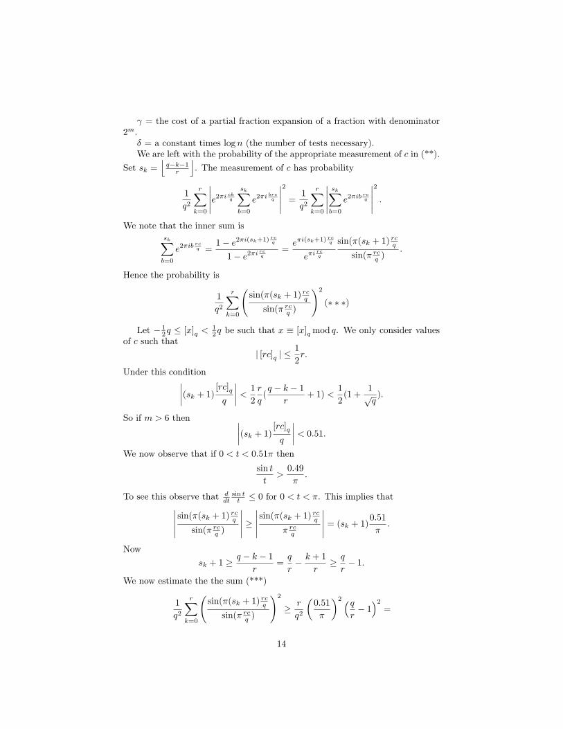
γ = the cost of a partial fraction expansion of a fraction with denominator2m.

δ = a constant times log n (the number of tests necessary).We are left with the probability of the appropriate measurement of c in (**).

Set sk =⌊q−k−1r

⌋. The measurement of c has probability

1

q2

r∑k=0

∣∣∣∣∣e2πi ckqsk∑b=0

e2πibrcq

∣∣∣∣∣2

=1

q2

r∑k=0

∣∣∣∣∣sk∑b=0

e2πibrcq

∣∣∣∣∣2

.

We note that the inner sum issk∑b=0

e2πibrcq =

1− e2πi(sk+1)rcq

1− e2πircq

=eπi(sk+1)

rcq

eπircq

sin(π(sk + 1) rcqsin(π rcq )

.

Hence the probability is

1

q2

r∑k=0

(sin(π(sk + 1) rcq

sin(π rcq )

)2(∗ ∗ ∗)

Let − 12q ≤ [x]q <12q be such that x ≡ [x]q mod q. We only consider values

of c such that| [rc]q | ≤

1

2r.

Under this condition∣∣∣∣(sk + 1)[rc]qq

∣∣∣∣ < 1

2

r

q(q − k − 1

r+ 1) <

1

2(1 +

1√q

).

So if m > 6 then ∣∣∣∣(sk + 1)[rc]qq

∣∣∣∣ < 0.51.

We now observe that if 0 < t < 0.51π then

sin t

t>

0.49

π.

To see this observe that ddtsin tt ≤ 0 for 0 < t < π. This implies that∣∣∣∣∣ sin(π(sk + 1) rcq

sin(π rcq )

∣∣∣∣∣ ≥∣∣∣∣∣ sin(π(sk + 1) rcq

π rcq

∣∣∣∣∣ = (sk + 1)0.51

π.

Now

sk + 1 ≥ q − k − 1

r=q

r− k + 1

r≥ q

r− 1.

We now estimate the the sum (***)

1

q2

r∑k=0

(sin(π(sk + 1) rcq

sin(π rcq )

)2≥ r

q2

(0.51

π

)2 (qr− 1)2

=

14

r

(0.49

π

)2(1

r− 1

q

)2thus if n is large we can absorb the 1

q in the constant and have the estimate(0.48

π

)21

r.

We also note that if | [rc]q | < 12r then there exists d such that

|rc− dq| < r

2

and dividing both sides by rq we have∣∣∣∣ cq − d

r

∣∣∣∣ < 1

2q.

We note that this argument is reversable. So it is equivalent to

| [rc]q | ≤1

2r.

Now if 0 < d < r then we can find 0 < c < r such that∣∣∣ cq − d

r

∣∣∣ < 12q . Let φ be

the number of 0 < d < r such that d and r are relatively prime (Euler’s Totientfunction). Then we have shown that the probability of measureing c such that

there exists d relatively prime to r with∣∣∣ cq − d

r

∣∣∣ < 12q is at least a constant times

φ(r)r . Now there are various lower bounds to

φ(r)r we will explain the one that

Shor uses in the second appendix to this subsection. The first will prove theneeded property of continued fractions.

3.2.1 Appendix1. Continued fractions

In this appendix we prove the characterization of a convergent of the continuedfraction that Shor uses. The reason we give details is that the characterizationis usually given for irrational numbers. Our argument involves a first stepthat allows the more standard method to work for rational numbers. We alsobegin the dsicussion with the observation that for rational numbers continuedfractions are calculated using the Euclidean algorithm. If q0,q1, q, ... are positivereal numbers then we define the symbol [q0, q1, q2, ..., qm] recursively by

[q0] = q0

and[q0,q1, ..., qm+1] = q0 +

1

[q1, ..., qm+1].

15

Thus[q0, q1, q2, q3, q4] = q0 +

1

q1 + 1q2+

1

q3+1q4

.

Suppose that 0 < a < b are integers we consider the Euclidean algorithm tocalculate gcd(a, b).

b = aq1 + r1, 0 ≤ r1 < a, r1 ∈ Z≥0.

If r1 = 0 then a = gcd(a, b) ortherwise r1 > 0 so

a = r1q2 + r2, 0 ≤ r2 < r1, q2 ∈ Z>0, r2 ∈ Z≥0.

If r2 = 0 then r1 = gcd(a, b) and otherwise

r1 = r2q3 + r3.0 ≤ r3 < r2, q3 ∈ Z>0, r3 ∈ Z≥0.

Euclid’s argorithm eventually stops at

rk−1 = rkqk

and according to the algrithm rk = gcd(a, b). The amazing part of this algorithmis that

[0, q1, ..., qk] =a

b

in lowest terms.For example a = 25, b = 90 then the algorithm yields:

q1 = 3, r1 = 15; q2 = 1, r2 = 10; q3 = 1, r3 = 5; q4 = 2; r4 = 0.

So gcd(25, 90) = 5 and a direct calculation shows that

[0, 3, 1, 1, 2] =5

18.

Thus the Euclidean algorithm gives an algorithm that calculates for 0 < a < bintegers, ab in lowest terms in the form

[0, q1, q2, ..., qk]

with qk ∈ Z>0. This is the continued fractions decomposition of ab . One cancheck that

[q0,q1, q2, ..., qk, 1] = [q0, q1, q2, ..., qk + 1].

It turns out that this is the only ambiguity in expressing a rational number asa continued fraction. Thus we will use the outcome of the Euclidean algorithmas “the”continued fraction expansion. For 1 < r ≤ k terms

[0, q1, ..., qr]

are called the convergents of the continued fraction expansion of ab .

16

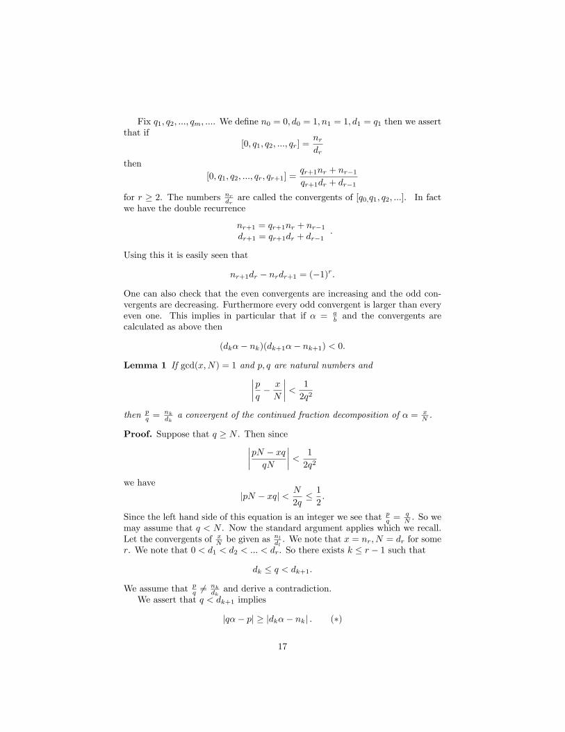
Fix q1, q2, ..., qm, .... We define n0 = 0, d0 = 1, n1 = 1, d1 = q1 then we assertthat if

[0, q1, q2, ..., qr] =nrdr

then[0, q1, q2, ..., qr, qr+1] =

qr+1nr + nr−1qr+1dr + dr−1

for r ≥ 2. The numbers nrdrare called the convergents of [q0,q1, q2, ...]. In fact

we have the double recurrence

nr+1 = qr+1nr + nr−1dr+1 = qr+1dr + dr−1

.

Using this it is easily seen that

nr+1dr − nrdr+1 = (−1)r.

One can also check that the even convergents are increasing and the odd con-vergents are decreasing. Furthermore every odd convergent is larger than everyeven one. This implies in particular that if α = a

b and the convergents arecalculated as above then

(dkα− nk)(dk+1α− nk+1) < 0.

Lemma 1 If gcd(x,N) = 1 and p, q are natural numbers and∣∣∣∣pq − x

N

∣∣∣∣ < 1

2q2

then pq = nk

dka convergent of the continued fraction decomposition of α = x

N .

Proof. Suppose that q ≥ N . Then since∣∣∣∣pN − xqqN

∣∣∣∣ < 1

2q2

we have

|pN − xq| < N

2q≤ 1

2.

Since the left hand side of this equation is an integer we see that pq = qN . So we

may assume that q < N . Now the standard argument applies which we recall.Let the convergents of xN be given as nldl . We note that x = nr, N = dr for somer. We note that 0 < d1 < d2 < ... < dr. So there exists k ≤ r − 1 such that

dk ≤ q < dk+1.

We assume that pq 6=nkdkand derive a contradiction.

We assert that q < dk+1 implies

|qα− p| ≥ |dkα− nk| . (∗)

17

Assuming this we complete the proof. We have

dk

∣∣∣∣α− nkdk

∣∣∣∣ ≤ q ∣∣∣∣α− p

q

∣∣∣∣ < 1

2q.

Hence ∣∣∣∣α− nkdk

∣∣∣∣ < 1

2qdk.∣∣∣∣pq − nk

dk

∣∣∣∣ =|dkp− nkq|

qdk≥ 1

qdk.

Thus1

qdk≤∣∣∣∣pq − nk

dk

∣∣∣∣ =

∣∣∣∣pq − α+ α− nkdk

∣∣∣∣ ≤∣∣∣∣pq − α∣∣∣∣+

∣∣∣∣α− nkdk

∣∣∣∣ < 1

2q2+

1

2dkq.

This implies that1

2dkq<

1

2q2

which says that dk > q which is a contradiction.We are left with the proof of (∗). We note that

det

[nk nk+1dk dk+1

]= (−1)k+1.

So the inverse to[nk nk+1dk dk+1

]is (−1)k+1

[dk+1 −nk+1−dk nk

]. Thus if

nku+ nk+1v = p,dku+ dk+1v = q

then(−1)k+1(dk+1p− nk+1q) = u,

(−1)k+1(−dkp+ nkq) = v.

Assert that we may assume uv 6= 0. If u = 0 then dk+1p = nk+1q.This impliesdk+1 divides q since gcd(nk+1, dk+1) = 1.But this contradicts the assumptionq < dk+1. If v = 0 we have nku = p and dku = q so

|qα− p| = |uqkα− upk| = |u| |dkα− nk| ≥ |dkα− nk| .

Thus we may assume uv 6= 0. We assert that uv < 0. Indeed, if uv > 0then, since q = dku + dk+1v, we would have q > dk+1 which is contrary to ourhypthesis. We have already observed that

(dkα− nk)(dk+1α− nk+1) < 0.

18

Now qα−p = (dku+dk+1v)α−(nku+nk+1v) = u(dkα−nk)+v(dk+1α−nk+1).This is a sum of terms that are of the same sign so

qα− p = ± (|u(dkα− nk)|+ |v(dk+1α− nk+1)|)

Thus

|qα− p| = |u| |(dkα− nk)|+ |v| |(dk+1α− nk+1)| ≥ |(dkα− nk)|

since u ∈ Z.

3.2.2 Appendix 2: Euler’s Totient function

If n is a positive integer then we set φ(n) equal to the number of integers0 < r < n with gcd(r, n) = 1. Clearly if n is prime then φ(n) = n − 1 and ifn = pk with p a prime φ(n) = pk−1(p− 1) = n(1− 1

p ). One can also show thatif gcd(m,n) = 1 then φ(mn) = φ(m)φ(n). So

φ(n) = n∏p|n

(1− 1

p

).

Proposition 2 There exists a constant C > 0 such that φ(n) ≥ C nlog log(n) if

(say) n > 3.

The argument basically the method of an exercise in [R]. Since the exerciseis only scetched out in [R] we give it a bit more detail here. We note that

log

(φ(n)

n

)=∑p|n

log(1− 1

p).

Since log(1− t) = −∑∞m=1

tm

m for |t| < 1we have log(1− t)+ t = −t2∑∞m=1

tm

m+1so if 0 < t < 1

log(1− t) = −t− t2∞∑m=0

tm

m+ 2

This implies that if 0 < t ≤ 12 then log(1− t) = −t+O(t2) thus∑

p|n

log(1− 1

p) > −

∑p|n

1

p+ C1

with C1 a constant. We now break up the sum as follows∑p|n

1

p=

∑p|n

p ≤ log n

1

p+

∑p|n

p > log n

1

p

19

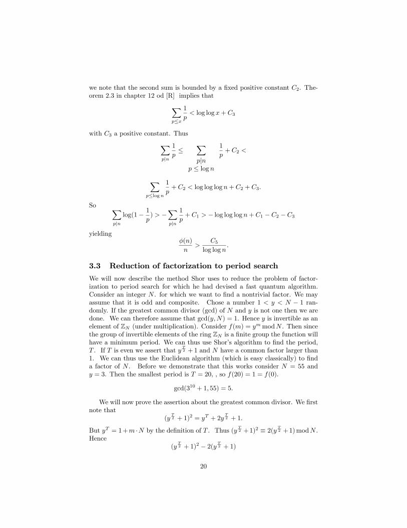
we note that the second sum is bounded by a fixed positive constant C2. The-orem 2.3 in chapter 12 od [R] implies that∑

p≤x

1

p< log log x+ C3

with C3 a positive constant. Thus∑p|n

1

p≤

∑p|n

p ≤ log n

1

p+ C2 <

∑p≤logn

1

p+ C2 < log log log n+ C2 + C3.

So ∑p|n

log(1− 1

p) > −

∑p|n

1

p+ C1 > − log log log n+ C1 − C2 − C3

yieldingφ(n)

n>

C5log log n

.

3.3 Reduction of factorization to period search

We will now describe the method Shor uses to reduce the problem of factor-ization to period search for which he had devised a fast quantum algorithm.Consider an integer N . for which we want to find a nontrivial factor. We mayassume that it is odd and composite. Chose a number 1 < y < N − 1 ran-domly. If the greatest common divisor (gcd) of N and y is not one then we aredone. We can therefore assume that gcd(y,N) = 1. Hence y is invertible as anelement of ZN (under multiplication). Consider f(m) = ym modN . Then sincethe group of invertible elements of the ring ZN is a finite group the function willhave a minimum period. We can thus use Shor’s algorithm to find the period,T . If T is even we assert that y

T2 + 1 and N have a common factor larger than

1. We can thus use the Euclidean algorithm (which is easy classically) to finda factor of N . Before we demonstrate that this works consider N = 55 andy = 3. Then the smallest period is T = 20, , so f(20) = 1 = f(0).

gcd(310 + 1, 55) = 5.

We will now prove the assertion about the greatest common divisor. We firstnote that

(yT2 + 1)2 = yT + 2y

T2 + 1.

But yT = 1 +m ·N by the definition of T . Thus (yT2 + 1)2 ≡ 2(y

T2 + 1) modN .

Hence(y

T2 + 1)2 − 2(y

T2 + 1)

20

is evenly divisible by N . We therefore see that((y

T2 + 1)− 2

)(yT2 + 1

)=(yT2 − 1

)(yT2 + 1

)is evenly divisible by N . Hence, if y

T2 + 1 and N have no common factor then

yT2 −1 is evenly divisible by N . This would imply that T2 (which is smaller than

T ) satisfies

f(x+T

2) = f(x).

This contradicts the choice of T as the minimal period. This is still not enoughto get a non-trivial divisor of N . We must still show that y can be chosen so thatN doesn’t divide y

T2 + 1 and that we can choose y so that T is even. Neither

can be done with certainty. What can be proved is that if N is not a pure primepower then the probability of choosing 1 < y < N −1 such that gcd(y,N) = 1,yhas even period and N doesn’t divide y

T2 + 1 is at least 3

4 . The proof of thisis will take us too far afield a good reference is [NC]. We note that classicallythe test whether a number, N , is a pure power of a number a > 2 and if so tocalculate the number is polynomial in the number of bits of N . The upshotis that a quantum computer will factor a number with very large probability(if the algorithm is done say 10 times then the probability of success would be0.999999 in polynomial time).

3.4 Error correction

So far we have ignored several of the diffi culties that we had indicated in section1 having to do with two problems that are caused by the environment. Thefirst is that we can only really look at mixed states since we cannot compute theactual action of the environment and the second is the decoherence caused by thedynamics of the total system. We will assume that our quantum computationsare divided into steps that take so little time that our initial pure states remainclose enough to being pure states that we can ignore the first diffi culty. Forthe second we will look at the decoherence over this small period as a smallerror. For most of the systems that are proposed the most likely error is a onequbit error. Thus as in classical error correction we will show how to set up aquantum error correcting code that corrects a one qubit error. The standardprocedure is to encode a qubit as an element of a two dimensional subspace ofa higher qubit space.That is we take V to be the space of n qubits and we take u0 and u1

orthonormal in V and assign

a |0〉+ b |1〉 7→ au0 + bu1.

The right hand side will be called the encoded qubit. The question is what isthe most likely error if we transmit the encoded qubit? The generally acceptedanswer is that it would be a transformation of the form

E = I⊗· · ·⊗A⊗· · ·⊗I

21

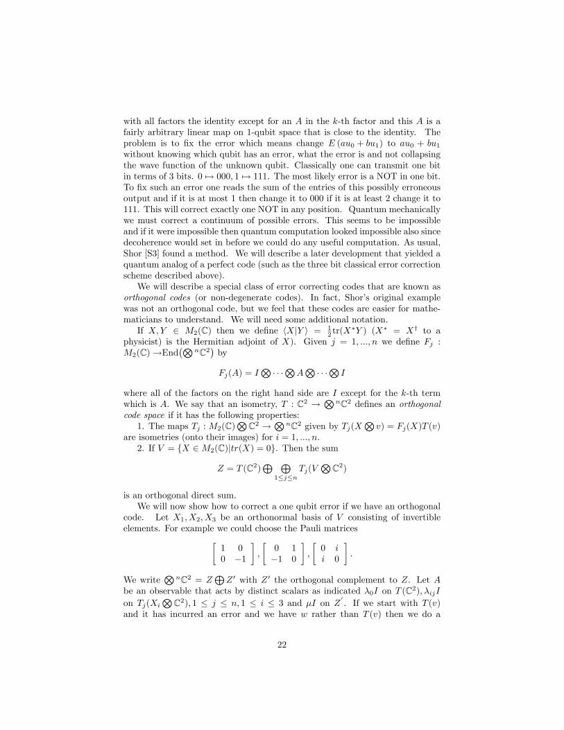
with all factors the identity except for an A in the k-th factor and this A is afairly arbitrary linear map on 1-qubit space that is close to the identity. Theproblem is to fix the error which means change E (au0 + bu1) to au0 + bu1without knowing which qubit has an error, what the error is and not collapsingthe wave function of the unknown qubit. Classically one can transmit one bitin terms of 3 bits. 0 7→ 000, 1 7→ 111. The most likely error is a NOT in one bit.To fix such an error one reads the sum of the entries of this possibly erroneousoutput and if it is at most 1 then change it to 000 if it is at least 2 change it to111. This will correct exactly one NOT in any position. Quantum mechanicallywe must correct a continuum of possible errors. This seems to be impossibleand if it were impossible then quantum computation looked impossible also sincedecoherence would set in before we could do any useful computation. As usual,Shor [S3] found a method. We will describe a later development that yielded aquantum analog of a perfect code (such as the three bit classical error correctionscheme described above).We will describe a special class of error correcting codes that are known as

orthogonal codes (or non-degenerate codes). In fact, Shor’s original examplewas not an orthogonal code, but we feel that these codes are easier for mathe-maticians to understand. We will need some additional notation.If X,Y ∈ M2(C) then we define 〈X|Y 〉 = 1

2 tr(X∗Y ) (X∗ = X† to a

physicist) is the Hermitian adjoint of X). Given j = 1, ..., n we define Fj :M2(C)→End

(⊗nC2

)by

Fj(A) = I⊗· · ·⊗A⊗· · ·⊗I

where all of the factors on the right hand side are I except for the k-th termwhich is A. We say that an isometry, T : C2 →

⊗nC2 defines an orthogonal

code space if it has the following properties:1. The maps Tj : M2(C)

⊗C2 →

⊗nC2 given by Tj(X

⊗v) = Fj(X)T (v)

are isometries (onto their images) for i = 1, ..., n.2. If V = {X ∈M2(C)|tr(X) = 0}. Then the sum

Z = T (C2)⊕ ⊕

1≤j≤nTj(V

⊗C2)

is an orthogonal direct sum.We will now show how to correct a one qubit error if we have an orthogonal

code. Let X1, X2, X3 be an orthonormal basis of V consisting of invertibleelements. For example we could choose the Pauli matrices[

1 00 −1

],

[0 1−1 0

],

[0 ii 0

].

We write⊗

nC2 = Z⊕Z ′ with Z ′ the orthogonal complement to Z. Let A

be an observable that acts by distinct scalars as indicated λ0I on T (C2), λijIon Tj(Xi

⊗C2), 1 ≤ j ≤ n, 1 ≤ i ≤ 3 and µI on Z

′. If we start with T (v)

and it has incurred an error and we have w rather than T (v) then we do a

22

measurement of A on w. If the measurement is µ then with high probabilitythe error wasn’t a one qubit error. Otherwise we assume a one qubit error thenthere is j such that w = Tj(X

⊗v). X = aI + bX1 + cX2 + dX2. Thus with

probability 1 the eigenvalue will be one of λ0, λ1j , λ2j , λ3j . If it is λ0 then w willhave collapsed to v. If it is λij then if w collapses to z then Fj(X

−1i )z = T (v)

we have thus corrected the error.Obviously, to use this idea we must have a way of finding T . We note first

of all that dimZ ≤ 2n and dimZ = 6n + 2 . If 6n + 2 ≤ 2n then n ≥ 5 andif n = 5 then 25 = 6 · 5 + 2. Thus the smallest n that we could use would ben = 5. We will now give conditions on a map T that are equivalent to havingan orthogonal code. If w ∈

⊗nC2 then w =

∑wj |j〉. Let 0 ≤ p < q < n be

two bit positions. Then we form a 4× 2n−2 matrix as follows. The i = i0 + i12,j = j0 + j12 + ...+ jn−32

n−3 entry is wk where

k = j0+...jp−12p−1+i02

p+jp2p+1+...+jq−22

q−1+i12q+jq−12

q+1+...+jn−32n−1.

If p = 0, q = 1 this is just k = i0 + i12 + 22(j0 + j12 + ... + jn−32n−3). Let

W (p, q, w) denote this matrix. We have

Theorem 3 T : C2 →⊗

nC2 defines an orthogonal code if and only if

W (p, q, T |i〉)W (p, q, T |j〉)∗ =1

4δi,jI.

For all p, q and i, j ∈ {0, 1}.This can be written as a system of quadratic equations. If we put them into

Mathematica for n = 5 the first solution is given as follows: We define

〈j1j2j3j4j5〉 = |j1j2j3j4j5〉+|j5j1j2j3j4〉+|j4j5j1j2j3〉+|j3j4j5j1j2〉+|j2j3j4j5j1〉 .Then set

T |0〉 =1

4(|0000〉+ 〈11000〉 − 〈10100〉 − 〈11110〉)

andT |1〉 =

1

4(|11111〉+ 〈00111〉 − 〈01011〉 − 〈00001〉) .

Because of the symmetry it is easy to check that the condition of the theoremis satisfied. This code was originally found by other methods (c.f. [KL]).

References[Co] D. Coppersmith, An approximate Fourier Transform Useful in Quantum

Factoring,arXiv:quant-ph/0201067v1.[NC] Michael Nielson and Isaac Chang, Quantum Computation and Quan-

tum Information, Cambridge University Press, Cambridge, 2000.[S3] P. Shor, A scheme for reducing decoherence in quantum computer mem-

ory, Phys. Rev. A,52,1995.[KL] E. Kroll and R. Laflamme, A theory of quantum error correcting codes,

Phys. Rev. A, 50:900-911,1997.[R] H. E. Rose, A Course in Number Theory, Second Edition, Oxford Science

Publications,Oxford, 1994.

23

4 Entanglement

As we have seen the only non-trivial reversible one bit operation is NOT whichinterchanges 0 and 1. We have made the simplifying assumption that all onequbit unitary operators are easily implementable on a quantum computer. Theoperation NOT gives rise to the unitary operator in one qubit with matrix[

0 11 0

]relative to the computational basis |0〉 , |1〉. We will say that a transformationof n bits that is given by applying either NOT or the identity to each bit is aclassical local transformation. A quantum local transformation in n qubits is aunitary operator of the form

A1⊗A2⊗· · ·⊗An

where Ai ∈ U(2). There is a major distinction between the classical and thequantum cases. The classical local transformations act transitively on the set ofall n bit bit strings. Whereas the quantum local transformations act transitivelyonly in the case when n = 1. For example there is no local transformation thattakes the state

|00〉+ |11〉√2

to |00〉 (see the next section for a proof). We will call a state that is not a productstate (not in the orbit of |00〉 under local transformations) an entangled state.The two code words of the five bit error correcting code are entangled. Further-more, entanglement explains some of the apparent paradoxes that appeared inthe early thought experiments of quantum mechanics. It is also basic to quan-tum teleportation (a subject that we will not be covering in these sections). Inthis section we will study the orbit structure of the local transformations onthe pure states and in particular functions that help to separate these orbits:the measures of entanglement. We will emphasize methods that allow one todetermine if two states are related by a local transformation and to determinethe extent of the entanglement of a state.

4.1 Measures of entanglement

We will first look at the example of an entangled state: |00〉+|11〉√2

. One way that

one can see that it is entangled is by observing that if we act on C2⊗C2 by

G = SL(2,C)×SL(2,C) by the tensor product action. Then G leaves invarianta symmetric form, the tensor product of the symplectic forms on each of the C2factors that are SL(2,C) invariant. This form, ( , ), is given by

(|00〉 , |11〉) = (|11〉 , |00〉 = 1,

(|01〉 , |10〉) = (|10〉 , |01〉) = −1

24

and all the other products are 0. We note that ( |00〉+|11〉√2

, |00〉+|11〉√2

) = 1 and(|00〉 , |00〉) = 0 so there can’t be a local transformation taking one to anothersince the function φ(u) = |(u, u)| is invariant under local transformations. It isan example of a measure of entanglement. Indeed, one can prove that a state,u,in 2 qubits is entangled if and only if φ(u) > 0. Another property enjoyed bythis function is that for all pure 2 qubit states φ(u) ≤ 1 and φ(u) = 1 if and onlyif u is in the orbit of |00〉+|11〉√

2under local transformations. To prove the upper

bound we consider u = a |00〉+ b |01〉+ c |10〉+ d |11〉. Then φ(u) = 2(ad− bc).Since 2|a||d| ≤ |a|2 + |d|2 we have |φ(u)| ≤ |a|2 + |b|2 + |c|2 + |d|2 = 1. Althoughit is not hard to prove the assertion about the orbit directly we will use a resultof Kempf and Ness [KN] which is useful in other contexts. For those of you whoare unfamiliar with semisimple Lie groups take G to be the product of n copiesof SL(2,C) and K to be n copies of SU(2).

Theorem 4 Let G be a semisimple Lie group over C and let K be a maximalcompact subgroup of G. Let (π, V ) be a finite dimensional holomorphic rep-resentation of G with the K-invariant Hilbert space structure 〈 | 〉. If v ∈ Vand m = inf{〈π(g)v|π(g)v〉 |g ∈ G}. Then if u ∈ π(G)v and 〈u|u〉 = m thenπ(K)u = {w ∈ π(G)v| 〈w|w〉 = m}. Furthermore the infimum is actually at-tained if and only if the orbit π(G)v is closed.

In words this says that the elements of minimal norm in a G orbit form asingle K-orbit.We will now give an idea of the proof. We note that Lie(G) = Lie(K) +

iLie(K). We therefore have

G = K exp(iLie(K)).

If X ∈ iLie(K) then dπ(X)∗ = dπ(X). Thus

d2

dt2〈π(exp tX)v|π(exp tX)v〉

= 4 〈dπ(X)π(exp tX)v|dπ(X)π(exp tX)v〉 ≥ 0

With equality if and only if dπ(X)v = 0. Everything follows from this.We will now show how the Kempf-Ness result applies to our situation for

2 qubits. We first note that relative to G = SL(2,C)×SL(2,C) the spaceV = C2

⊗C2 has the following orbit structure. For each λ ∈ C − {0} the set

Mλ = {w ∈ V |(v, v) = λ} is a single orbit. The other orbits are π(G) |00〉and {0}. The union of the latter two is M0. We set u0 = |00〉+|11〉√

2. We note

that we have Mλ = zπ(G)u0 with z2 = λ. We therefore see that the elementsin the unit sphere that maximize φ are contained in the set of elements theform w = eiθ π(g)u0

‖π(g)u0‖ , g ∈ G. For such a w we have φ(w) = 1‖π(g)u0‖2

. Thus

maximizing φ on the unit sphere means (up to phase) minimizing the norm onπ(G)u0. The Kempf-Ness theorem implies that this subset of π(G)u0 is π(K)u0.This completes the proof of the assertion.

25

We note that the group of local transformations on⊗

nC2 is the imageof S1 × SU(2)n with S1 the circle group acting by scaler multiplication andSU(2)n acting by the tensor product action (i.e. by local transformations). Wewill therefore concentrate on invariants for SU(2)n. We also note that if weconsider φ(u)2 rather than φ(u) then it is a polynomial function on C2

⊗C2

as a real vector space. We will only consider measures of entanglement thatare polynomials invariant under K = SU(2)n on

⊗nC2 as a real vector space.

We will use the term measure of entanglement for such a polynomial. We willdenote the algebra of such polynomials by PR(

⊗nC2)K . These are exactly

what we need to separate the K-orbits.

Theorem 5 If u, v ∈⊗

nC2 then u ∈ π(K)v if and only if f(u) = f(v) for allf ∈ PR(

⊗nC2)K .

We also note that if we look at the action of the circle group by multiplicationon⊗

nC2 we can define a Z-grading on PR(⊗

nC2)K by f ∈ PjR(⊗

nC2)K iff ∈ PR(

⊗nC2)K and f(zu) = zjf(u) for all z ∈ S1 and u ∈

⊗nC2.

Theorem 6 If u, v ∈⊗

nC2 then u ∈ S1π(K)v if and only if f(u) = f(v) forall f ∈ P0R(

⊗nC2)K .

Both of these theorems are consequences of the following result.

Theorem 7 Let U be a compact Lie group. Let (ρ,W ) be a finite dimensionalrepresentation of U on a real Hilbert space. Let P(W )U be the algebra of allcomplex valued polynomials on W that are invariant under U . If u, v ∈W thenu ∈ ρ(U)v if and only if f(u) = f(v) for all f ∈ P(W )U .

Proof. The necessity is obvious. Since v 7→ ‖v‖2 is in P(W )U we will prove thatif ‖v‖ = ‖u‖ = r > 0 and f(u) = f(v) for all f ∈ P(W )U then u ∈ ρ(U)v. TheStone-Weierstrauss theorem implies that the restriction of P(W ) to the sphereof radius r,Sr,is uniformly dense in the space of continuous functions on Sr.Suppose that ρ(U)v ∩ ρ(U)u is empty then Uryson’s Lemma implies there is acontinuous function ϕ on Sr such that ϕ|ρ(U)v ≡ 1 and ϕ|ρ(U)u ≡ 0. The uniform

density implies that there exists an f ∈ P(W ) such that |f(x) − ϕ(x)| < 14 for

all x ∈ Sr. Let du denote normalized invariant measure on U . We definef(x) =

∫U

f(ρ(z)x)dz. Then f ∈ P(W )U . We have

|f(v)− 1| =∣∣∣∣∫U

f(ρ(z)v)dz − 1

∣∣∣∣ ≤ ∫U

|f(ρ(z)v)dz − ϕ(ρ(z)v)|dz ≤ 1

4

hence |f(v)| > 34 similarly |f(u)| < 1

4 . This proves the theorem.

4.2 Three qubits

These results make it reasonable to assert that the orbit of |00〉+|11〉√2

under localtransformations consists of the most entangled two qubit states. In the case of 3

26

qubits there is a similar result. First the ring of invariant (complex polynomials)on C2

⊗C2⊗C2 under the tensor product action of

G = SL(2,C)×SL(2,C)×SL(2,C)

is generated by one element, f , of degree 4 (here we will be stating severalresults without proof in this case the details can be found in [GrW]). We candefine it as follows: If v ∈ C2

⊗C2⊗C2 the we can write it as

v = |0〉⊗v0 + |1〉

⊗v1

with v0, v1 ∈ C2⊗C2. If we use the symmetric form defined above we have

f(v) = det

[(v0, v0) (v0, v1)(v1, v0) (v1, v1)

].

As in the case of two qubits most of the orbits under G are described by thevalues of f . Here we set Mλ = {v ∈ C2

⊗C2⊗C2|f(v) = λ}. Then if λ 6= 0

we have Mλ consists of a single orbit. If λ = 0 then there are 6 orbits in M0,

We note that f( |000〉+|111〉√2

) = 14 . Thus Mλ = zG

(|000〉+|111〉√

2

)with z4 = 4λ.

We will now describe the orbits in M0. First there is the open orbit in thisquartic given as the orbit of

w0 =|001〉+ |010〉+ |100〉√

3.

If we remove this orbit fromM0 then there are three open orbits in what remains.They are the orbits of |000〉+|011〉√

2, |000〉+|101〉√

2and |000〉+|110〉√

2. If in addition these

are removed then what we have left is the union of 0 and the product states(which form a single orbit).One can show by an argument similar to that in two qubits that if u is

a state then |f(u)| ≤ 14 and if uo = |000〉+|111〉√

2then f(uo) = 1

4 . Since the

set where f is non-zero is exactly the set of all elemets C×G(|000〉+|111〉√

2

)we

see that if u is a state with |f(u)| 6= 0 then u = guo‖guo‖ with g ∈ G. Thus

f(u) = f(

guo‖guo‖

)= 1‖guo‖4

f(guo) = 14‖guo‖4

. Thus the set of states with

|f(u)| = 14 are exactly the elements that minimize the value of ‖guo‖

4 for g ∈ G.Thus Theorem 2 implies:

Proposition 8 If K = S1SU(2)×SU(2)×SU(2) then

{v ∈ C2⊗C2⊗C2||f(v)| = 1

4, ‖v‖ = 1} = K

(|000〉+ |111〉√

2

).

Thus one value of one invariant is enough to determine if a state can begotten from |000〉+|111〉√

2by local transformations. For example

v =|111〉+ |001〉+ |010〉+ |100〉

2

27

has the property that f(v) = 14 . So it can be obtained by a local transformation

from |000〉+|111〉√2

.So far we have been analyzing only one polynomial measure of entangle-

ment. There is the natural problem of determining a generating set for thesemeasures. To do this it is useful to reduce the problem to a problem involvingcomplex algebraic groups and complex polynomials. The basic idea is that if Gis a simply connected semi-simple Lie group over C then G is a linear algebraicgroup. If K is a maximal compact subgroup of G and if (ρ, V ) is a finite dimen-sional unitary representation of K then ρ extends to a regular representationof G on V . The real polynomials on V are the complex polynomials in boththe bra and the ket vectors. The ket vectors give a copy of V as a complexvector space whereas the ket vectors give a copy of the complex dual representa-tion of V . This implies that the algebra PR(V )K is naturally isomorphic withP(V

⊕V ∗)G. In the case when we are dealing with qubits the representation

of G = SL(2)n on⊗

nC2 is self dual. We are thus looking at the problem ofdetermining the invariants of G acting on two copies of

⊗nC2 by the diagonal

action. We analyze this problem for two and three qubits.

4.3 Measures of entanglement for two and three qubits

We first look at 2 qubits and continue the discussion begun in the previoussubsection. As we have observed G = SL(2,C)×SL(2,C) leaves invarianta symmetric bilinear form on C2

⊗C2. A dimension count shows that the

image of G on C2⊗C2 is the full orthogonal group for this form. Thus the

action on C2⊗C2 can be interpreted as the action of SO(4,C) on C4. We

are thus looking at the invariants of SO(4,C) on two copies of C4. Classicalinvariant theory implies that the algebra of invariants is generated by the threepolynomials α(v

⊕w) = (v, v), β(v

⊕w) = (v, w) and γ(v

⊕w) = (w,w), This

implies

Lemma 9 The algebra of measures of entanglement in 2 qubits is the set ofpolynomials in (v, v), 〈v|v〉 and (v, v).

Thus in this case we were using the only “interesting”measure, since we areonly considering states which are assumed to satisfy 〈v|v〉 = 1.

The situation is different for three qubits. We will describe a set of gener-ators in this case that was determined in [MW1] our method is a modificationwhich is an outgrowth of joint work with H. Kraft. As above we look uponC2⊗C2⊗C2 as C2

⊗C4 and G = SL(2,C)×SL(2,C)×SL(2,C) acting as

SL(2,C)×SO(4,C). For the moment we will ignore the SL(2,C) factor andlook at I

⊗SO(4,C) acting on two copies of C2

⊗C4. If we consider only the

action of SO(4,C) then we are looking at its action on 4 copies of C4. Welook at this as SO(4,C) acting on X ∈ M4(C) under right multiplication bythe transpose of the matrix. Then the invariants for SO(4,C) are generatedby the matrix entries of XXT (the upper T stands for transpose) and det(X)(for these results and others stated without proof in this subsection please see

28

[GW]). We now look at the action of the remaining SL(2,C). The SL(2,C) isacting on the left on the matrix via multiplication by the block diagonal matrix

h =

[g 00 g

].

Thus the SL(2,C) factor is acting on the generators of the SO(4,C) invariantstrivially on γ = detX (an invariant under the full G of degree 4) and viahXXThT with h as above, We write XXT in block form[

A BBT C

]then the SL(2,C) is acting on the components via A 7→ gAgT , B 7→ gBgT , C 7→gCgT . We note that A and C are symmetric and completely general and B isan arbitrary 2× 2 matrix which we can write as

a

[0 1−1 0

]+ Z

with Z a general two by two symmetric matrix. The coeffi cient a defines an in-variant forG of degree 2 on the qubits which we will call α. The rest of the actionis by three copies of the action of SL(2,C) on the symmetric 2×2 matrices. Us-ing the trace form we see that this is just the action of SO(3,C) on three copiesof C3. Again we look upon this as the action of SO(3,C) on Y = M3(C) via leftmultiplication. The invariants in this case are generated by β = detY (an invari-ant of degree 6 on the qubits) and the matrix coeffi cients of Y TY which yield 6invariants of degree 4. The upshot is the invariants are generated by an invariantof degree 2 (α), an invariant of degree 4 (γ), an invariant of degree 6 (β) and 6invariants of degree 4 (the matrix coeffi cients of Y TY ), µ1, ..., µ6. We note thatthe invariants γ and β have the property that their squares are invariant underO(3)×O(4). Thus γ2 and β2 are in the algebra generated by α and µ1, ..., µ6. Wecan also see from the invariant theory of SO(3) that the functions α, µ1, ..., µ6are algebraically independent. We therefore see that the full ring of invariantsis C[α, µ1, .., µ6]

⊕C[α, µ1, .., µ6]β

⊕C[α, µ1, .., µ6]γ

⊕C[α, µ1, .., µ6]βγ.

References[GrW] Benedict H. Gross and Nolan R. Wallach, On quaternionic discrete

series and their continuations, J. Reine Angew. Math. 481 (1996),73-123.[GW] Roe Goodman and Nolan R. Wallach, Representations and invariants

of the classical groups, Cambridge University Press, Cambridge, 1998.[MW1] David Meyer and Nolan Wallach, Invariants for multiple qubits: the

case of 3 qubits. Mathematics of quantum computation,77—97, Comput. Math.Ser., Chapman & Hall/CRC, Boca Raton, FL, 2002.[KN] George Kempf and Linda Ness, The length of vectors in representa-

tion spaces. Algebraic geometry (Proc. Summer Meeting, Univ. Copenhagen,Copenhagen, 1978), pp. 233—243, Lecture Notes in Math., 732, Springer, Berlin,1979.

29

5 Four and more qubits

In the cases of 2 and 3 qubits it is fairly clear what the maximally entangledstates should be or at least there are just a few candidates for that honor. Wewill see that there is an immense variety of states that are highly entangled inthe case of 4 qubits. This and the calculation of Hilbert series for measuresof entanglement (see subsection 5.2) indicate that the search for all measuresof entanglement or the complete description of the orbit structure for arbitrarynumbers of qubits will be so hard and complicated as to become useless. How-ever the case of 4 qubits gives some indications of how to find more invariants.Also, methods similar to the Kempf-Ness theorem can be used to prove unique-ness theorems (for example the theorem of Rains [R] that implies that the 5 biterror correcting code we discussed earlier is unique up to local transformations).As it turns out the orbit structure under

G = SL(2,C)×SL(2,C)×SL(2,C)×SL(2,C) on C2⊗C2⊗C2⊗C2

can be determined using the results of Kostant and Rallis [KR]. Since it fits intheir theory in case of the symmetric pair (SO(4, 4), SO(4) × SO(4)). We willnow describe the outgrowth of this theory purely in terms of qubits.

5.1 Four qubits

We are therefore analyzing the action of G = SL(2) × SL(2) × SL(2) × SL(2)on the space V = C2

⊗C2⊗C2⊗C2 via the tensor product action

(g1, g2, g3, g4)(v1⊗

v2⊗

v3⊗

v4) = g1v1⊗

g2v2⊗

g3v3⊗

g4v4

We first note that if H = SL(2)×SL(2) and if W = C2⊗C2 and if we have H

act onW by the tensor product action then there is a H-invariant non-degeneratesymmetric bilinear form, (..., ...), on W given as follows

(v⊗

w, x⊗

y) = ω(v, x)ω(w, y).

Here ω((x1, y1), (x2, y2)) = x1y2 − x2y1. This form allows us to define a linearmap, T , of V onto End(W ) in the following way

T (v1⊗

v2⊗

v3⊗

v4)(w1⊗

w2) = ω(v3, w1)ω(v4, w2)v1⊗

v2.

We look upon G as H ×H. Thus if g = (h1, h2) then

T (gv)(w) = h1T (v)(h−12 w).

If A ∈ End(W ) then we define A# by (Aw1, w2) = (w1, A#w2). We note that

if h ∈ H then h# = h−1. This implies that

T (gv)T (gv)# = h1T (v)h−12 (h1T (v)h−12 )#

= h1T (v)h−12 h2T (v)#h−11 = h1T (v)T (v)#h−11 .

30

We therefore have invariants f2j(v) = tr((T (v)T (v)#)j), j = 1, 2, ... and g4(v) =det(T (v)).

Theorem 10 The ring of invariants under the action of G on V is generatedby the algebraically independent elements f2, f4, g4, f6.

The following discussion gives a sketch of a proof.We will use qubit notation for elements of V . Thus V has a basis consisting

of elements |i0i1i2i3〉 with ij = 0, 1. We set

v1 =1

2(|0000〉+ |1111〉+ |0011〉+ |1100〉),

v2 =1

2(|0000〉+ |1111〉 − |0011〉 − |1100〉),

v3 =1

2(|1010〉+ |0101〉+ |0110〉+ |1001〉),

v4 =1

2(|1010〉+ |0101〉 − |0110〉 − |1001〉).

These states can be described in terms of the Bell states for 2 qubits. Letu± = |00〉±|11〉√

2and v± = |01〉±|10〉√

2then

v1 = u+⊗u+, v2 = u−

⊗u−, v3 = v+

⊗v+, v4 = v−

⊗v−.

We note that if v = x1v1 + x2v2 + x3v3 + x4v4 then

T (v) =

x1−x22 0 0 x1+x2

20 x4−x3

2 −x3+x42 00 −x3+x42

x4−x32 0

x1+x22 0 0 x1+x2

2

.Hence

f2j(v) =∑

x2ji

andg4(v) = x1x2x3x4.

We note that this implies that the functions f2, f4, g4, f6 are algebraically in-dependent. Set a = {v = x1v1 + x2v2 + x3v3 + x4v4|xj ∈ C} and a′ = {v =x1v1 + x2v2 + x3v3 + x4v4|xi 6= ±xj for i 6= j}. One can check that the mapG×a′ → V given by g, v 7−→ gv is regular. Furthermore, if x ∈ a′ then the set ofg ∈ G such that gx = x is finite. Since dimG = 12 and dim a = 4 we see that iff is a G invariant polynomial then f is completely determined by its restrictionto a (since Gg′ has interior). We also note that if N = {g ∈ G|ga = a} then thegroupW = N|a is the subgroup of the group generated by the linear maps givenby the permutations of v1, v2, v3, v4 and those that involve an even number ofsign changes. For example,([

0 ii 0

],

[1 00 1

],

[0 ii 0

],

[1 00 1

])

31

corresponds to v1 → v3, v2 → v4, v3 → v1, v4 → v2,(1√2

[1 1−1 1

],

1√2

[1 1−1 1

],

1√2

[1 1−1 1

],

1√2

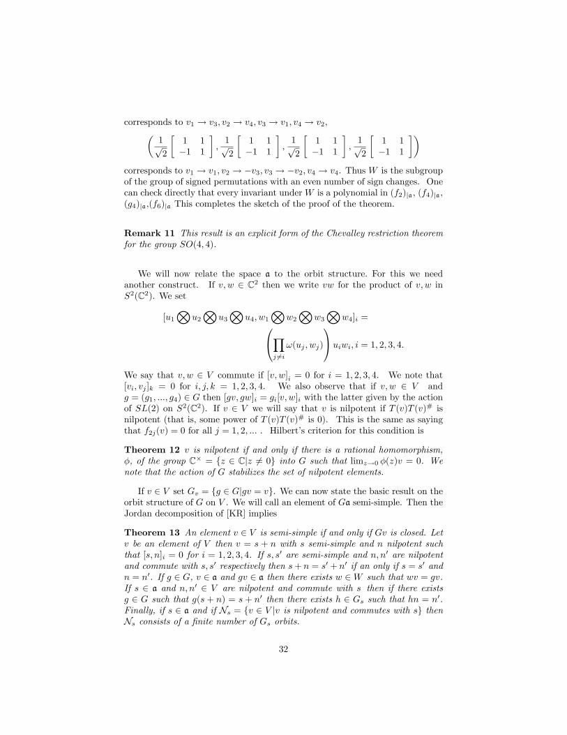
[1 1−1 1

])corresponds to v1 → v1, v2 → −v3, v3 → −v2, v4 → v4. Thus W is the subgroupof the group of signed permutations with an even number of sign changes. Onecan check directly that every invariant underW is a polynomial in (f2)|a, (f4)|a,(g4)|a,(f6)|a This completes the sketch of the proof of the theorem.

Remark 11 This result is an explicit form of the Chevalley restriction theoremfor the group SO(4, 4).

We will now relate the space a to the orbit structure. For this we needanother construct. If v, w ∈ C2 then we write vw for the product of v, w inS2(C2). We set

[u1⊗

u2⊗

u3⊗

u4, w1⊗

w2⊗

w3⊗

w4]i =∏j 6=i

ω(uj , wj)

uiwi, i = 1, 2, 3, 4.

We say that v, w ∈ V commute if [v, w]i = 0 for i = 1, 2, 3, 4. We note that[vi, vj ]k = 0 for i, j, k = 1, 2, 3, 4. We also observe that if v, w ∈ V andg = (g1, ..., g4) ∈ G then [gv, gw]i = gi[v, w]i with the latter given by the actionof SL(2) on S2(C2). If v ∈ V we will say that v is nilpotent if T (v)T (v)# isnilpotent (that is, some power of T (v)T (v)# is 0). This is the same as sayingthat f2j(v) = 0 for all j = 1, 2, ... . Hilbert’s criterion for this condition is

Theorem 12 v is nilpotent if and only if there is a rational homomorphism,φ, of the group C× = {z ∈ C|z 6= 0} into G such that limz→0 φ(z)v = 0. Wenote that the action of G stabilizes the set of nilpotent elements.

If v ∈ V set Gv = {g ∈ G|gv = v}. We can now state the basic result on theorbit structure of G on V . We will call an element of Ga semi-simple. Then theJordan decomposition of [KR] implies

Theorem 13 An element v ∈ V is semi-simple if and only if Gv is closed. Letv be an element of V then v = s + n with s semi-simple and n nilpotent suchthat [s, n]i = 0 for i = 1, 2, 3, 4. If s, s′ are semi-simple and n, n′ are nilpotentand commute with s, s′ respectively then s+ n = s′ + n′ if an only if s = s′ andn = n′. If g ∈ G, v ∈ a and gv ∈ a then there exists w ∈W such that wv = gv.If s ∈ a and n, n′ ∈ V are nilpotent and commute with s then if there existsg ∈ G such that g(s + n) = s + n′ then there exists h ∈ Gs such that hn = n′.Finally, if s ∈ a and if Ns = {v ∈ V |v is nilpotent and commutes with s} thenNs consists of a finite number of Gs orbits.

32

We will next give a quantitative version of this theorem. We will first estab-lish a bit more terminology.We will say that a nilpotent element, n, is regular if setting U = T (n)T (n)#,

R = T (n)# then R,RU+UR,RU2+U2R,RU3+U3R are linearly independentoperators. A family of such examples is

a |0011〉+ b |0100〉+ c |1001〉+ d |1010〉

with abcd 6= 0. It is easily seen that all of the regular elements of the aboveform are in the G orbit of the element with a, b, c, d all equal to 1. Let us callthis element no. It turns out that there are 4 distinct regular nilpotent orbits.There are 20 distinct nilpotent orbits. The general theory also allows us todetermine the general orbits. The number of different “types”of orbits is 90.The term “type”will become clear in the course of the discussion below leadingto an explanation of the quantitative statement.For each i = 1, 2, 3, 4 we define εi ∈ V ∗ by εi(vj) = δij . Let Φ = {±(εi +

εj)|1 ≤ i < j ≤ 4} ∪ {εi − εj |1 ≤ i 6= j ≤ 4}. Set ∆ = {α1 = ε1 − ε2, α2 =ε2 − ε3, α3 = ε3 − ε4, α4 = ε3 + ε4}. If s ∈ a then we define Φs = {α ∈Φ|α(s) = 0}. One can show that if s ∈ a then there exists w ∈ W such thatΦws = Φ ∩ spanZ(∆ ∩Φws). The main theorem implies that we need only lookat elements s satisfying

Φs = Φ ∩ spanZ(∆ ∩ Φs).

Here are the possibilities with |∆ ∩ Φs| ≤ 1.∆ ∩ Φs = ∅, s = x1v1 + x2v2 + x3v3 + x4v4, xi 6= ±xj for all i 6= j.∆ ∩ Φs = {α1}, s = x1(v1 + v2) + x3v3 + x4v4, xi 6= ±xj for all i 6= j.∆ ∩ Φs = {α2}, s = x1v1 + x2(v2 + v3) + x4v4, xi 6= ±xj for all i 6= j.∆ ∩ Φs = {α3}, s = x1v1 + x2v2 + x3(v3 + v4), xi 6= ±xj for all i 6= j.∆ ∩ Φs = {α4}, s = x1v1 + x2v2 + x3(v3 − v4), xi 6= ±xj for all i 6= j.We note that the permutation (123) maps the set {s|s = x1(v1+v2)+x3v3+

x4v4, xi 6= ±xj} for all i 6= j bijectively onto the set {s|s = x1v1 +x2(v2 + v3) +x4v4, xi 6= ±xj for all i 6= j}. Similarly, there is a permutation that maps the setindicated by ∆ ∩ Φs = {α2} onto the set indicated by ∆ ∩ Φs = {α3}. Finally,the sign change v1 → v1, v2 → −v2, v3 → v3, v4 → −v4 takes the set indicatedby ∆∩Φs = {α3} onto the set indicated by ∆∩Φs = {α4}. Thus by the basictheorem we need only consider the first two in our list. For |∆∩Φs| ≥ 2 we willonly list the cases up to the action of signed permutations involving an evennumber of sign changes. Here are all of the examples1. ∆ ∩ Φs = ∅, s = x1v1 + x2v2 + x3v3 + x4v4, xi 6= ±xj for all i 6= j.2. ∆ ∩ Φs = {α1}, s = x1(v1 + v2) + x3v3 + x4v4, xi 6= ±xj for all i 6= j.3. ∆ ∩ Φs = {α1, α2}, s = x1(v1 + v2 + v3) + x4v4, x1 6= ±x4.4. ∆ ∩ Φs = {α1, α3}, s = x1(v1 + v2) + x3(v3 + v4), x1 6= ±x3.5. ∆ ∩ Φs = {α1, α4}, s = x1(v1 + v2) + x3(v3 − v4), x1 6= ±x3.6. ∆ ∩ Φs = {α1, α2, α3}, s = x1(v1 + v2 + v3 + v4), x1 6= 0.7. ∆ ∩ Φs = {α1, α2, α4}, s = x1(v1 + v2 + v3 − v4), x1 6= 0.8. ∆ ∩ Φs = {α2, α3, α4}, s = x1v1, x1 6= 0.

33

9. ∆ ∩ Φs = {α1, α3, α4}, s = x1(v1 + v2), x1 6= 0.10. ∆ ∩ Φs = {α1, α2, α3, α4}, s = 0.

We now count the number of Gs orbits in Ns in each of the 10 cases above.Case 1. Yields 1 since Ns = {0}. 2. Yields 2. 3. Yields 3. 4. and 5. Yield 8.6.,7.,8.Yield 7. 9. Yields 27. 10. Yields 20. The total is our promised 90.

Here are some examples. The extremes in part 10. of the list involving thenon-zero orbits are the 4 regular nilpotent orbits and the orbit of product states

{u1⊗u2⊗u3⊗u4|ui ∈ C2 − {0}}.

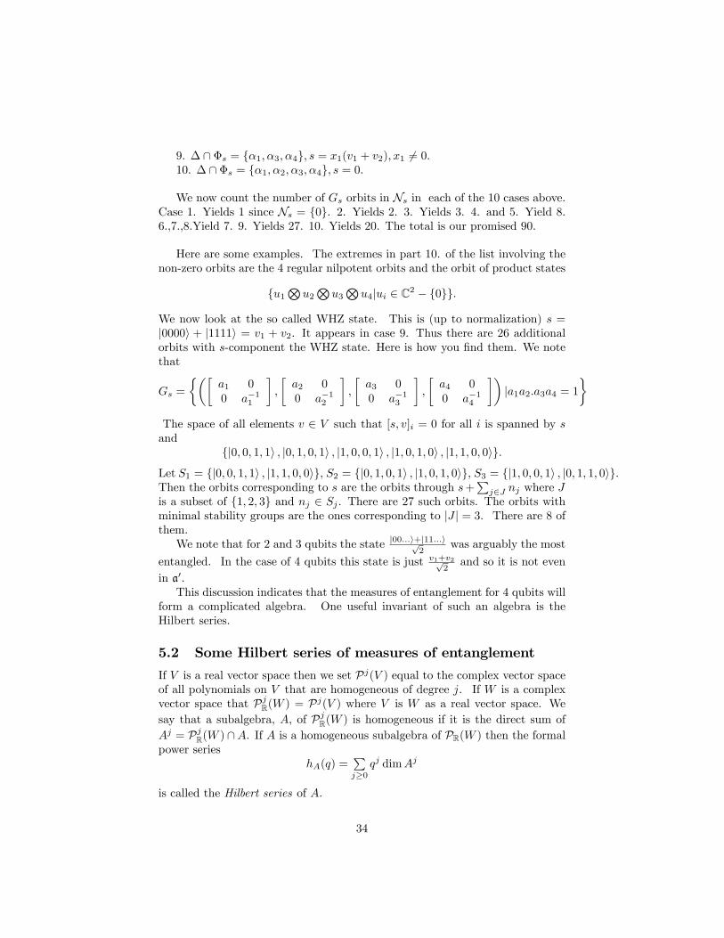
We now look at the so called WHZ state. This is (up to normalization) s =|0000〉 + |1111〉 = v1 + v2. It appears in case 9. Thus there are 26 additionalorbits with s-component the WHZ state. Here is how you find them. We notethat

Gs =

{([a1 00 a−11

],

[a2 00 a−12

],

[a3 00 a−13

],

[a4 00 a−14

])|a1a2.a3a4 = 1

}The space of all elements v ∈ V such that [s, v]i = 0 for all i is spanned by sand

{|0, 0, 1, 1〉 , |0, 1, 0, 1〉 , |1, 0, 0, 1〉 , |1, 0, 1, 0〉 , |1, 1, 0, 0〉}.

Let S1 = {|0, 0, 1, 1〉 , |1, 1, 0, 0〉}, S2 = {|0, 1, 0, 1〉 , |1, 0, 1, 0〉}, S3 = {|1, 0, 0, 1〉 , |0, 1, 1, 0〉}.Then the orbits corresponding to s are the orbits through s+

∑j∈J nj where J

is a subset of {1, 2, 3} and nj ∈ Sj . There are 27 such orbits. The orbits withminimal stability groups are the ones corresponding to |J | = 3. There are 8 ofthem.We note that for 2 and 3 qubits the state |00...〉+|11...〉√

2was arguably the most

entangled. In the case of 4 qubits this state is just v1+v2√2and so it is not even

in a′.This discussion indicates that the measures of entanglement for 4 qubits will

form a complicated algebra. One useful invariant of such an algebra is theHilbert series.

5.2 Some Hilbert series of measures of entanglement

If V is a real vector space then we set Pj(V ) equal to the complex vector spaceof all polynomials on V that are homogeneous of degree j. If W is a complexvector space that PjR(W ) = Pj(V ) where V is W as a real vector space. Wesay that a subalgebra, A, of PjR(W ) is homogeneous if it is the direct sum ofAj = PjR(W ) ∩A. If A is a homogeneous subalgebra of PR(W ) then the formalpower series

hA(q) =∑j≥0

qj dimAj

is called the Hilbert series of A.

34

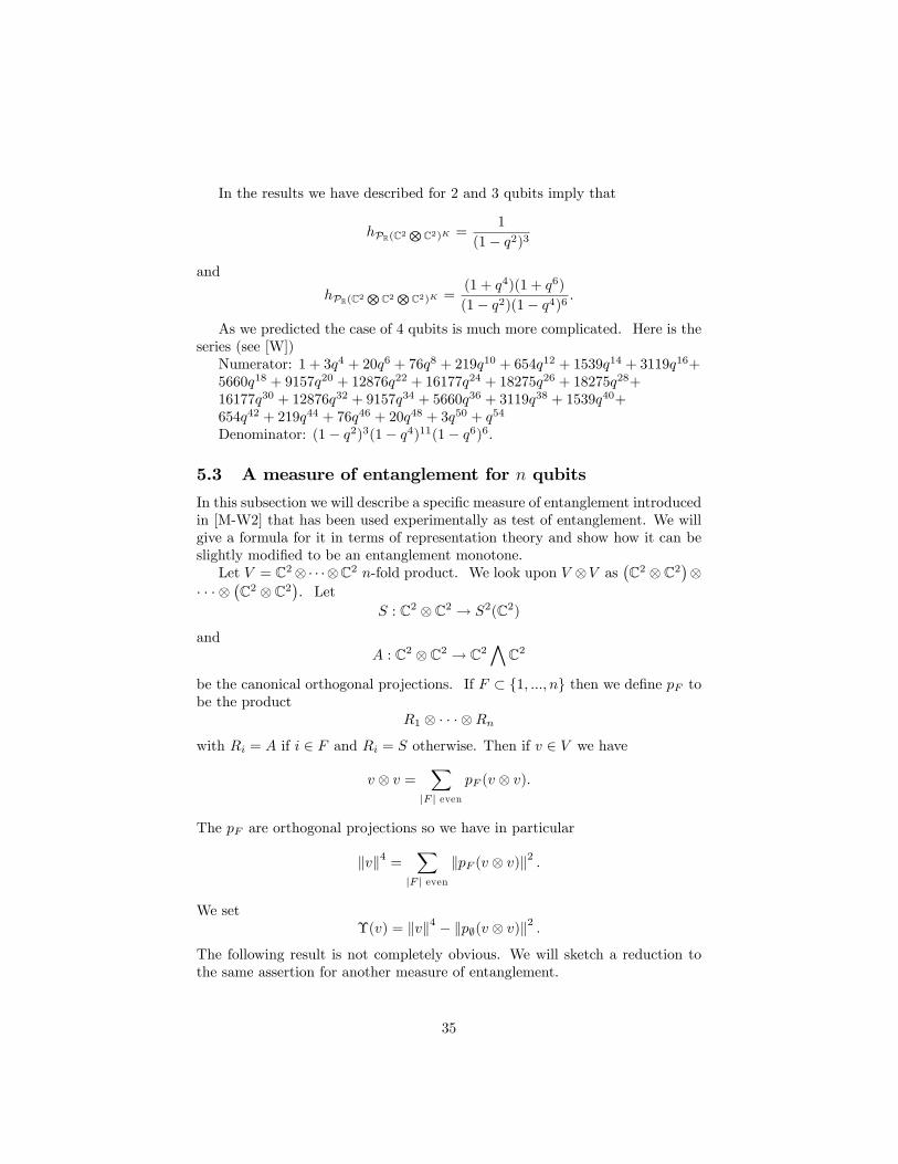
In the results we have described for 2 and 3 qubits imply that

hPR(C2⊗C2)K =

1

(1− q2)3

and

hPR(C2⊗C2⊗C2)K =

(1 + q4)(1 + q6)

(1− q2)(1− q4)6 .

As we predicted the case of 4 qubits is much more complicated. Here is theseries (see [W])Numerator: 1 + 3q4 + 20q6 + 76q8 + 219q10 + 654q12 + 1539q14 + 3119q16+5660q18 + 9157q20 + 12876q22 + 16177q24 + 18275q26 + 18275q28+16177q30 + 12876q32 + 9157q34 + 5660q36 + 3119q38 + 1539q40+654q42 + 219q44 + 76q46 + 20q48 + 3q50 + q54

Denominator: (1− q2)3(1− q4)11(1− q6)6.

5.3 A measure of entanglement for n qubits

In this subsection we will describe a specific measure of entanglement introducedin [M-W2] that has been used experimentally as test of entanglement. We willgive a formula for it in terms of representation theory and show how it can beslightly modified to be an entanglement monotone.Let V = C2⊗· · ·⊗C2 n-fold product. We look upon V ⊗V as

(C2 ⊗ C2

)⊗

· · · ⊗(C2 ⊗ C2

). Let

S : C2 ⊗ C2 → S2(C2)

andA : C2 ⊗ C2 → C2

∧C2

be the canonical orthogonal projections. If F ⊂ {1, ..., n} then we define pF tobe the product

R1 ⊗ · · · ⊗Rnwith Ri = A if i ∈ F and Ri = S otherwise. Then if v ∈ V we have

v ⊗ v =∑|F | even

pF (v ⊗ v).

The pF are orthogonal projections so we have in particular

‖v‖4 =∑|F | even

‖pF (v ⊗ v)‖2 .

We setΥ(v) = ‖v‖4 − ‖p∅(v ⊗ v)‖2 .

The following result is not completely obvious. We will sketch a reduction tothe same assertion for another measure of entanglement.

35

Theorem 14 A state v ∈ V is a product state if and only if Υ(v) = 0.

This measure of entanglement is related to one denoted Q in [MW-2] (theyare the same for 2 and 3 qubits) and which was defined as follows. If 0 ≤ j <

N = 2n and j =n−1∑m=0

jm2m then if 0 ≤ i < n define ti(j) =∑

0≤m<ijm2m +∑

i<m<n

jm2m−1. If v =∑

0≤j<Nvj |j〉 then we set vi,0 =

∑ji=0

vj |ti(j)〉 and vi,1 =∑ji=1

vj |ti(j)〉. Thus if

v =|111〉+ |001〉+ |010〉+ |100〉

2

then

v2,0 =|01〉+ |10〉

2, v2,1 =

|00〉+ |11〉2

.

We set Q(v) =n−1∑i=0

‖vi,0∧vi,1‖2. Here in W

⊗W , u

∧w =

u⊗

w−w⊗

u

2 and

we use the tensor product inner product. We note that Q(|000〉+|111〉√

2

)= 3

8 and

Q(|001〉+|010〉+|100〉√

3

)= 1

3 . One can show that if v ∈⊗

nC2 then

Q(v) =

n2∑

k=1

k∑|F |=2k

∥∥∥pF (v⊗

v)∥∥∥2 .

We note that in [MW-2] we proved that the (relatively easy) result thatthe Theorem above is true for Q replacing Υ. Since Q(v) = 0 if and only if‖pF (v

⊗v)‖2 = 0 for all |F | > 0 and Υ has the same property. Hence Υ(v) = 0

if and only if Q(v) = 0.In a forthcoming article we will prove that Υ is an entanglement monotone.

This assentially means that quantum operations (such as measurements andlocal transformations) cannot increase its value. This condition is sometimesincluded in the definition of a measure of entanglement.

References[KR] B. Kostant and S. Rallis, Orbits and Lie group representations associ-

ated to symmetric spaces, Amer. J. Math.,93(1971),753-809.[MW2] David Meyer and Nolan Wallach, Global entanglement in multipar-

ticle systems. Quantum information theory. J. Math. Phys. 43 (2002), no. 9,4273—4278.[R] Erik Rains, Quantum codes of minimum distance two. IEEE Trans.

Inform. Theory 45 (1999), no. 1, 266—271.[W] Nolan R. Wallach, The Hilbert series of measures of entanglement for 4

qubits, Acta Appl. Math. 86 (2005), no.1-2,203-220.

36