7. The Hartree-Fock Self-Consistent Field (SCF) Method

Contents

Total Hamiltonian of an atom or molecule, Born-Oppenheimer approximation,General aspects of Hartree-Fock method, self-consistent field, basis function. Central ConceptsSelf-consistent field, correlation, basis function, configuration interaction.

Difficult Points

Inclusion of electron correlation in energy/state calculation.Mathematical procedures in the theoretical formulation.

Notes

First, we define the problem, beginning with the Schrödinger equation

Our goal is to come up with an analytic equation for the energy which can be minimized with respect to some variational parameter(s) to give an upper bound on the energy. To do this, we must

a. Understand the hamiltonian operater . b. Find an appropriate wave function which allows simple calculation of the electronic

energy. c. Examine potential variational parameters to figure out how to minimize the energy.

1. The Hamiltonian,

The Hamiltonian is the total energy operator for a system, and is written as the sum of the kinetic energy of all the components of the system and the internal potential energy. In an atom or molecule, comprised of positive nuclei and negative electrons, the potential energy is simply that due to the coulombic interactions present. Thus for the kinetic energy in a system of

M nuclei and N electrons:

And for the potential energy:

Since ,

Within the Born-Oppenheimer approximation, we assume the nuclei are held fixed while the electrons move really fast around them. (note:

.) In this case, nuclear motion and electronic motion are

seperated. The last two terms can be removed from the total hamiltonian

to give the electronic hamiltonian, , since , and . The nuclear motion is handled in a rotational/vibrational analysis. We will be working within the B-O approximation, so realizing

we completly define the problem. Solving the electronic Schrödinger equation using this will give the electronic structure of a molecular system at a fixed nuclear geometry.

2. The Wave Function,

We've derived a complete many-electron Hamiltonian operator. Of course, the Schrödinger equation involving it is intractable, so let's consider a simpler problem, involving the one-electron hamiltonian

which involves no electron-electron interaction. This soluable in the B-O approximation (recall the hydrogen atom by letting M=1). Call the solutions

to the one-electron Schrödinger equation . These will be atomic/molecular spin orbitals when we get around to it, but for now let it suffice to know they satisify the eigenequation

with the interpretation that electron i occupies spin orbital with energy

. If we ignore electron-electron interaction in , we construct a simpler system with Hamiltonian

It will have eigenfunctions which are simple products of occupied spin orbitals, and thus an energy which is a sum of individual orbital energies, as

 

This kind of wavefunction is called a Hartree Product, and it is not physically realistic. In the first place, it is an independent-electron model, and we know electrons repel each other. Secondly, it does not satisfy the antisymmetry principle due to Pauli which states that the sign of the wavefunction must be inverted under the operation of switching the coordinates of any two electrons, or

Part of the proof of equation 13 acknowledges this is not so for a Hartree Product. To remedy this, first consider a two-electron system, such as helium. Two equivalent Hartree Product wavefunctions for this system are

Obviously, neither of these is appropriate. However, using the old ``by inspection...'' trick, we notice that

does. The mathematical form of this wavefunction can be generated by a determinant of 's,

 

The familiar Pauli exclusion principle follows directly from this example. When we attempt to doubly occupy a spin orbital by putting electron 1 and electron 2 in it, what happens?

Equation 17 can be generalized to give the N electron Slater determinant  

A shorthand notation for a Slater determinant has been introduced, where all the diagonal elements in the determinant are written in order as a ``ket'' vector. Equation 19 can thus be written as

where the normalization constant is absorbed into the notation. Now we have written down a wave function appropriate for use in the case where . In HF theory, we make some simplifications so many-

electron atoms and molecules be treated this way. By tacitly assuming that each electron moves in a perceived electric field generated by the

stationary nuclei and the average spatial distribution of all the other electrons, it essentially becomes an independant-electron problem. The HF Self Consistent Field procedure (SCF) will be bent on constructing each

to give the lowest energy.

3. Energy Expressions

Let's assume a wave function of the Slater determinant form and find an expression for the expectation value of the energy. We've written a Slater determinant as a ket vector in shorthand notation, allowing us to make use of Dirac notation for such things as overlap. In this context, recall that

where the basis vectors is expanded in are every possible value of x with

contraction coefficients identified as the value of at x. Thus placing an

operator (such as ) inside the bracket, we get the expectation value of the observable associated with that operator. Since is the energy operator,

is the differential of all the spin and space coordinates of all the electrons. With much foresight, we continue to simplify the problem by writing as a sum of one- and two-electron operators

This will allow us to more precisely develop the electronic energy by its components.

First, examine the core hamiltonian .

The nature of this is best evidenced by example, so we turn to the familiar

helium atom, . Look at one term in the above sum, for

the sake of illustration take .

  

Here is defined as . In the first two terms of equation 28, the integrations over electron two's coordinates can be carried out irrespective of electron one's, and give the two terms of equation 29. The last two terms integrate to zero due to the orthogonality

of and . Repeating this for we get exactly the same thing, and we see

Profound, isn't it? Seems that every occupied spin orbital yields a term of

the form to the one electron energy.

Now look at .

Continuing to work in the helium atom example (realize that this could be two electron system) pick (i,j) = (1,2) and look at that one term.

 

Unfortunately, the operator prevents separation of the integrations over the electronic coordinates of electron 1 and electron 2. It cannot be assured that the last two terms are zero. In general, they are not. However, since the and are dummy variables, the first and second terms of equation

33 are equal, as are the last two. Thus for the two electron operator ,

where

The construction is called an antisymmetrized two electron integral in physicists notation. By working in the spin orbital basis, much trouble is avoided. In fact, by extending the results shown previously to the general case, we can now

write down the HF energy for a given set of occupied spin orbitals.  

Now move on and consider working in the spatial orbital basis, where

This is more natural, since our intuition is usually based on having a region of space which describes the location (more or less) of electrons, one of alpha spin and one of beta spin. Some of quantum chemistry is formulated entirely in terms of spin orbitals, for various reasons. For our purposes, we will work entirely in the spatial orbital basis. This will cause things to get somewhat murky soon, but in the long run it will be simpler. At any rate, in the two electron system we adore so much, we can identify the two occupied spin orbitals and as the spin up and spin down halves of the single lowest lying spatial orbital, a 1s in helium or the bonding orbital in H for example. These can be more precisely defined as

This changes the way we write slater determinants. Using an overbar to

denote spin occupation of a spatial orbital, ,

Rethinking the one electron integrals for this case,

The notation is used to denote an integral over only spatial coordinates, what remains after the spin integrations have been carried out, giving a factor of 1 or 0. That was a neat closed shell system. How about something like

?

where supercript ‘occ’ stands for “occupied”, ‘docc’ for “double occupied” and ‘socc’ for “single occupied”.

The coefficient here is related to the occupation of spatial orbital i, and

will be more precisely defined later. The two electron integrals are a little more involved, but we go about it in essentially the same manner.

(Does anybody find equations 53-56 hard to derive?)Yes, I know. Very confusing. But it's all just notation, and can be understood. In physicist's notation (equivalent to Dirac notation),

refers to the two electron integral where and are

functions of electron 1, while and are functions of electron 2. Chemist's

notation (with the square brackets []) places the functions of electron 1 on the left and the functions of electron 2 on the right. The most important fact we need to obtain equations 53-56 is: When the two functions of a single electron are not of the same spin, the whole integral goes to zero, otherwise the spin integrates out to 1. Easy, isn’t it? Hence the spin-free

notation . What occurs when the two electrons are of parallel spin, requiring distinct spatial orbitals and a wavefunction something like

? The same general form is present, and a related antisymmetrized two electron integral is evaluated. In this case,

.

Another bit of notation, which should be apparent and

because we encountered them for a few times before: is termed a Coulomb integral and has the physically reassuring interpretation of somehow accounting for electronic repulsion between electrons in

atomic/molecular orbital i and atomic/molecular orbital j. , the exchange

integral, has no classical analog and no trivial physical interpretation. Many have tried to come up with something, and a typical attempt says that it ``correlates the motions of electron i and j when they have parallel spins, lowering the energy since those electrons avoid each other better.'' Whatever. Best to just move on to a general energy equation in the spatial MO basis. In summary:

The one electron integrals contribute for each electron in orbital i.

The two electron integrals contribute for each pair of electrons, and for

each pair of parallel spin.

4. What Variational Parameter?

Ah, the crux of the problem, is it not? Up until now, we've just assumed we

have some set of molecular orbitals or , which we can manipulate at

will. But how does one come up with even approximate solutions to the many body Schrödinger equation without having to solve it? Start with the celebrated linear combination of atomic orbitals to get molecular orbitals (LCAO-MO) approximation. This allows us to use some set of (approximate) atomic orbitals, the basis functions which we know and love, to expand the MOs in. In the most general terms,

remains a spatial molecular orbital, is a spatial atomic orbital (perhaps

symmetry orbital, but no matter), and are the contraction coefficients by which we transform from one basis to another. Armed with only this, we should be able to compose the electronic energy in the atomic orbital basis. Why, you ask? Because we have an expression in terms of integrals over MOs. To variationally minimize that energy, we need to vary the MOs themselves, but have no way to do that, since they remain these amorphous constructs. By defining them a bit more precisely, we should

arrive at a point where an obvious set of variational parameters (hint: ) present themselves. Begin with the closed shell HF energy in terms of spatial MOs.

Since and ,  

is a one electron integral over atomic orbitals. Do we have

something we can actually calculate!? Take an aside and examine this quantity superficially.

Typically, basis functions are constructed to mimic true atomic orbitals. The Hydrogen atom can be described rigorously, and the eigenfunctions found. The 1s orbital looks something like

. It satisfies all the appropriate boundary conditions, having a cusp at the nucleus and exponentially decaying to zero at infinity. Higher angular momentum functions, like 2p's and 3d's, can be built from this basic framework through adding the angular nodes by multiplying in factors of x, y, and z. Basis functions such as these are called slater-type orbitals(STO). If instead of the exponential we use a gaussian function,

, we loose the boundary conditions but generate a more tractable problem when it comes to calculating integrals. Using a linear combination of single cartesian gaussian-type orbitals (SGTO) to approximate a slater-type orbital gives better computational accuracy without too much more effort. Here's the functional forms of all three types:

Just taking a 1s SGTO for illustrative purposes, what is that one electron integral?

Hey! We can do that!

Back to the problem at hand, we now need to expand the two electron integrals in the MO basis. Following a procedure analogus to equation 64, we get

All of these AO integrals can be calculated and stored, to be called up when needed to evaluate the electronic energy. The closed shell energy in the AO basis can be written as

is the density matrix, a product of AO-MO coefficient matrices, or

5. Hartree Fock Equations

The electronic energy is a functional of the spin orbitals, and we want to minimize it subject to some set of constraints. This can be done using the calculus of variations applied to functionals. So lets look at a general example of functional variation applied to E, a functional of some trial wavefunction that can be linearly varied under a single constraint.

  

By equation 74, we see that , depending on the form of the

wavefunction, and by equation 75 that can be linearly expanded (hence linearly varied) in some set of N functions. This is directly analogous to expanding the asymmetric top rotational wavefunctions in a complete set of symmetric top rotational wavefunctions. The task is to minimize E subject to the single constraint that the wavefunction remain normalized, or

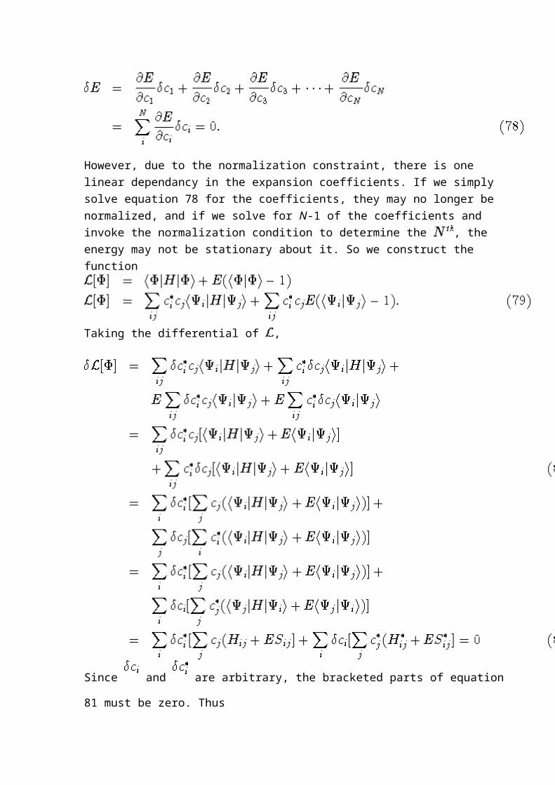
 Writing the energy as

we want , so  

However, due to the normalization constraint, there is one linear dependancy in the expansion coefficients. If we simply solve equation 78 for the coefficients, they may no longer be normalized, and if we solve for N-1 of the coefficients and invoke the normalization condition to determine the , the energy may not be stationary about it. So we construct the function

Taking the differential of ,  

Since and are arbitrary, the bracketed parts of equation 81 must be

zero. Thus

It is clear that this can be written as a matrix product, and is in fact an eigenvalue equation in the form

Knowing that H and S are hermetian, this matrix eigenvalue equation can be rewritten as

 

The matrix S HS is symmetric and easily diagonalized, with eigenvectors S c. These can be transformed (multiply on the left by S ) to give the optimal coefficients for stationary state. This is very powerful, since in one fell swoop we've got the entire energy spectrum and the appropriate wave functions, properly orthonormal, for all the states. This should illustrate the general technique we will be employing to develop the Hartree-Fock equations and from them the algebraic Roothaan equations, which you will be programming later. On to the true problem. Assume we have a wave function in the form of a

Slater determinant of spin orbitals, . We state the problem as:

Please minimize the electronic energy of this single determinant subject to the constraint that the spin orbitals all remain orthonormal to one another.

We already understand the energy fine by equation 37, and the constraint can be simply stated as

There are N spin orbitals, so there are N(N+1)/2 independent constraints (note:

), so we need that many undetermined multipliers in our lagrangian function, for which we present

 

The restricted sum will prove inconvenient, but it can be eliminated. By taking the

complex conjugate of the constraints and the lagrangian function, equation 86,

we realize we can unrestrict the summation by restraining to be a hermitian matrix, such that . This introduces no new undetermined multipliers into

the equation, and creates a form more amenable to further derivation. Thus the Lagrangian function we will be working with is

 

The differential of this function must be set to zero as before, giving us

Since we have an electronic energy in terms of spin orbitals

we can write the variance of the energy as

It takes some thought to realize that there are only two unique two electron integrals in this list, and that it can be written

The other variance we need is , which can be expanded as

So the whole thing boils down to one neat statement,

If we conveniently define a coulomb operator and an exchange operator

as

  we can rewrite the two electron integral

This allows for a more compact notation to be employed in writing the variance in the lagrangian function

Like before, the part in brackets is forced to be zero, since can be anything. Setting it equal to zero and rearranging to make it look like some sort of eigenvalue equation yields

These are the glorious Hartree-Fock equations derived in general in the spin orbital basis. But wait - there's a problem. These are coupled integro-differential equations, and while they are not strictly unsolvable, they're a pain. It would be

nice to at least uncouple them, so let's do that. If we apply a unitary rotation to the full set of spin orbitals, generating a new set

where U is unitary, ie. U = U , what changes? The rotation can be written as a matrix product, if we define A as the matrix resembling the slater

determinant for the system, ie. det(A) = . In that case,

However, since this matrix U is unitary, , and the new wavefunction differs from the old by a phase factor, affecting nothing observable. How does it affect f(1) and ?

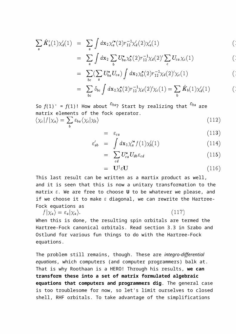
So f(1)' = f(1)! How about ? Start by realizing that are matrix elements of the fock operator.

This last result can be written as a martix product as well, and it is seen that this is now a unitary transformation to the matrix . We are free to choose U to be whatever we please, and if we choose it to make diagonal, we can rewrite the Hartree-Fock equations as

When this is done, the resulting spin orbitals are termed the Hartree-Fock canonical orbitals. Read section 3.3 in Szabo and Ostlund for various fun things to do with the Hartree-Fock equations.

The problem still remains, though. These are integro-differential equations, which computers (and computer programmers) balk at. That is why Roothaan is a HERO! Through his results, we can transform these into a set of matrix formulated algebraic equations that computers and programmers dig. The general case is too troublesome for now, so let's limit ourselves to closed shell, RHF orbitals. To take advantage of the simplifications this can afford, we need to return to the spatial orbital basis. We've derived the spin orbital based Fock operator

Without further ado, we'll introduce the spatial orbital based Fock operator and be done with it.    

With the properties

Now we introduce a basis set expansion to bring the HF integro-differential

equations to soluable algebraic equations. Letting ,

Multiplying by and integrating over electron 1 gives

Identifying the integrals as matrix elements of the fock operator and the unit operator (overlap) respectively,

Using the fact that is diagonal, this can be written as the matrix product  

So what is F, this so called Fock Matrix? We've defined before as the

matrix element of the one electron fock operator, f(1) in equation 119. Writing out this integral and expanding,  

This is a quantity which can be easily constructed given a set of molecular

orbitals (the coefficients ) and a precalculated set of atomic orbital

integrals. At this point, the Hartree-Fock equations have been reduced to a matrix eigenvector problem, , but not in a computationally convenient form. Following the analysis leading to equation 84, we first define the transformed Fock matrix as

We can then take

to be equivalent to equation 127. Since is diagonal by choice, diagonalizing the transformed Fock matrix gives a set of transformed molecular orbital coefficients, . The matrix can be back transformed to give the true MO coefficient matrix, . The density matrix for these coefficients is formed by the product , and can subsequently be used to construct a new fock matrix via equation 129. Since the overlap matrix does not depend on the MO coefficients, the same unitary transformation can be applied to the new fock matrix to give a new transformed fock matrix. This can be diagonalized to produce new MO coefficients, and the process repeated until convergance. As an initial guess for the fock matrix, one generally uses the core hamiltonian, ignoring all the two electron integrals.

From the core hamiltonian, an initial C is obtained and a much improved Fock matrix can be built including the two electron integrals. And that's about it for the Hartree-Fock Self Consistent Field Method. These last few pages will be the most important when you get around to programming the closed shell SCF method for the specific case of water, as you will be given the integrals in a file, and you can begin the process by building the core hamiltonian as described above.

Summary

In the Hartree-Fock SCF method, each electron is treated as independent and moves in a “potential field”. One starts from certain (simple!?) forms of wavefunction for the electrons (usually with spin orbitals or their linear combinations such as Slater determinants) and calculate the “potential field” created by the electrons in the initial states, then put the new “potential field” in the eigen equations of energy to calculate the new electron statesnew potential fieldnew state……until the iteration does not bring further improvement, i.e., when self-consistency of the wavefunction or potential field is reached.

ReferencesTextbook pp.305-318., pp.339-342, pp.426-436.Szabo and Ostlund: Modern Quantum Chemistry, rev. ed., McGraw-Hill, Dover, 1996.Back to lecture note indexBack to quantum chemistry II homeQuestions?Back to Ding’s home