quantum chemical studies of the chloride-based cvd process
TRANSCRIPT
1
Institutionen för fysik, kemi och biologi
Examenarbete
Quantum chemical studies of the chloride-based CVD process for
Silicon Carbide
Emil Kalered
14-06-12
LITH-IFM-A-EX--12/2618—SE
Linköpings universitet Institutionen för fysik, kemi och biologi
581 83 Linköping

2
Abstract In this report the interaction between SiH2 molecules and a SiC-4H (0001) surface and SiCl2 molecules and a SiC-
4H (0001) surface is investigated. This is done using a cluster model to represent the surface. First the clusters
are investigated by calculating some properties to compare with experimental data to motivate the use of the
cluster model. The band gap calculated by extrapolation for an infinitely large cluster is 3.75 eV which is fairly
close to the experimental value of 3.2 eV.
Adsorption studies are performed and the main conclusion is that the SiH2 molecule adsorbs more strongly on
the surface then the SiCl2 molecule, adsorption energies are calculated to approximately 200 kJ mol-1 and 100
kJ mol-1 respectively.
At the end a few migration studies are performed with the conclusion that SiCl2 more easily can diffuse on the
surface compared to the SiH2 molecule. The respective activation energies for migration on the surface are 4 kJ
mol-1 for SiCl2 and 87 kJ mol-1 for SiH2.
3
1. Introduction During the last twenty years the interest in silicon carbide based devices has greatly increased due to the
superior properties compared to conventional silicon based devices. For a comparison between different
semiconductors see table 1. But the drawback of silicon carbide (SiC) technology is the much more expensive
manufacturing costs. For a long time the production method used for manufacturing epitaxial layer of silicon
carbide has been the Chemical Vapor Deposition (CVD) process.
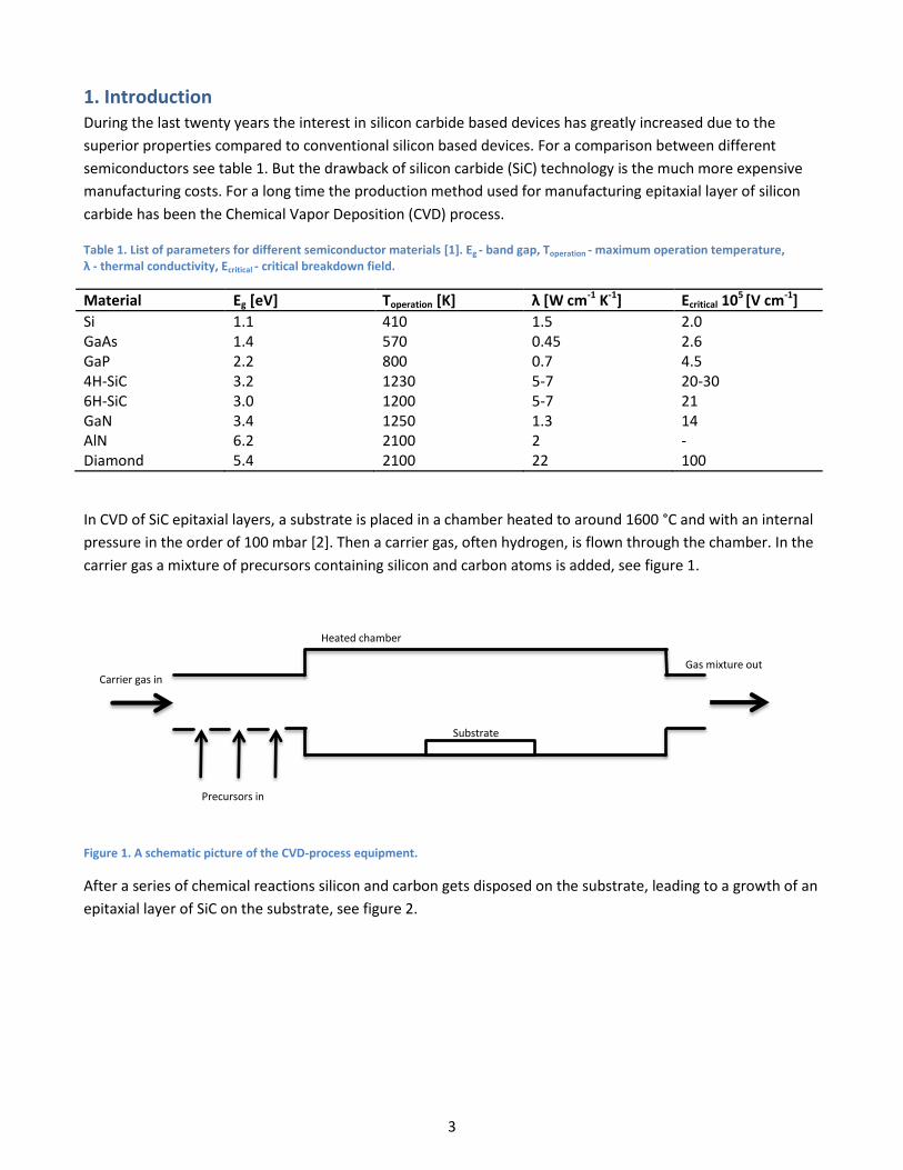
Table 1. List of parameters for different semiconductor materials [1]. Eg - band gap, Toperation - maximum operation temperature, λ - thermal conductivity, Ecritical - critical breakdown field.
Material Eg [eV] Toperation [K] λ [W cm-1 K-1] Ecritical 105 [V cm-1]
Si 1.1 410 1.5 2.0 GaAs 1.4 570 0.45 2.6 GaP 2.2 800 0.7 4.5 4H-SiC 3.2 1230 5-7 20-30 6H-SiC 3.0 1200 5-7 21 GaN 3.4 1250 1.3 14 AlN 6.2 2100 2 - Diamond 5.4 2100 22 100
In CVD of SiC epitaxial layers, a substrate is placed in a chamber heated to around 1600 °C and with an internal
pressure in the order of 100 mbar [2]. Then a carrier gas, often hydrogen, is flown through the chamber. In the
carrier gas a mixture of precursors containing silicon and carbon atoms is added, see figure 1.
Figure 1. A schematic picture of the CVD-process equipment.
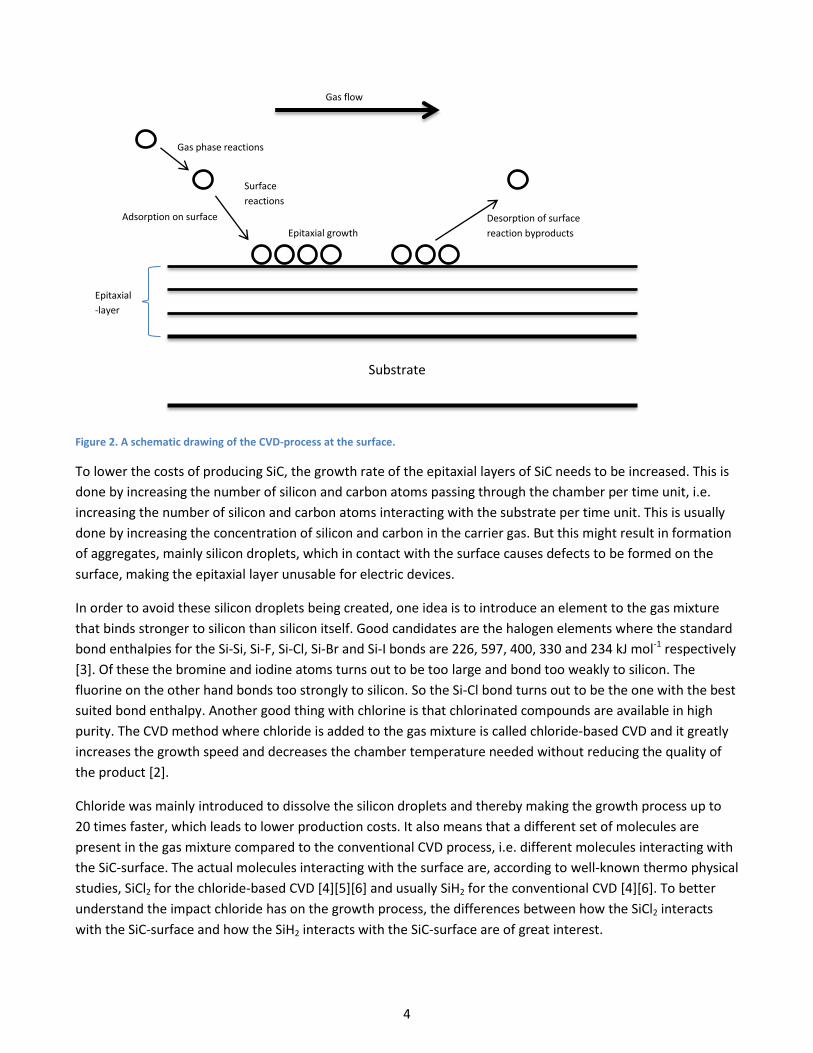
After a series of chemical reactions silicon and carbon gets disposed on the substrate, leading to a growth of an
epitaxial layer of SiC on the substrate, see figure 2.
Heated chamber
Substrate
Gas mixture out Carrier gas in
Precursors in
4
Figure 2. A schematic drawing of the CVD-process at the surface.
To lower the costs of producing SiC, the growth rate of the epitaxial layers of SiC needs to be increased. This is
done by increasing the number of silicon and carbon atoms passing through the chamber per time unit, i.e.
increasing the number of silicon and carbon atoms interacting with the substrate per time unit. This is usually
done by increasing the concentration of silicon and carbon in the carrier gas. But this might result in formation
of aggregates, mainly silicon droplets, which in contact with the surface causes defects to be formed on the
surface, making the epitaxial layer unusable for electric devices.
In order to avoid these silicon droplets being created, one idea is to introduce an element to the gas mixture
that binds stronger to silicon than silicon itself. Good candidates are the halogen elements where the standard
bond enthalpies for the Si-Si, Si-F, Si-Cl, Si-Br and Si-I bonds are 226, 597, 400, 330 and 234 kJ mol-1 respectively
[3]. Of these the bromine and iodine atoms turns out to be too large and bond too weakly to silicon. The
fluorine on the other hand bonds too strongly to silicon. So the Si-Cl bond turns out to be the one with the best
suited bond enthalpy. Another good thing with chlorine is that chlorinated compounds are available in high
purity. The CVD method where chloride is added to the gas mixture is called chloride-based CVD and it greatly
increases the growth speed and decreases the chamber temperature needed without reducing the quality of
the product [2].
Chloride was mainly introduced to dissolve the silicon droplets and thereby making the growth process up to
20 times faster, which leads to lower production costs. It also means that a different set of molecules are
present in the gas mixture compared to the conventional CVD process, i.e. different molecules interacting with
the SiC-surface. The actual molecules interacting with the surface are, according to well-known thermo physical
studies, SiCl2 for the chloride-based CVD [4][5][6] and usually SiH2 for the conventional CVD [4][6]. To better
understand the impact chloride has on the growth process, the differences between how the SiCl2 interacts
with the SiC-surface and how the SiH2 interacts with the SiC-surface are of great interest.
Surface
reactions
Gas flow
Epitaxial growth Desorption of surface
reaction byproducts Adsorption on surface
Gas phase reactions
Substrate
Epitaxial
-layer
5
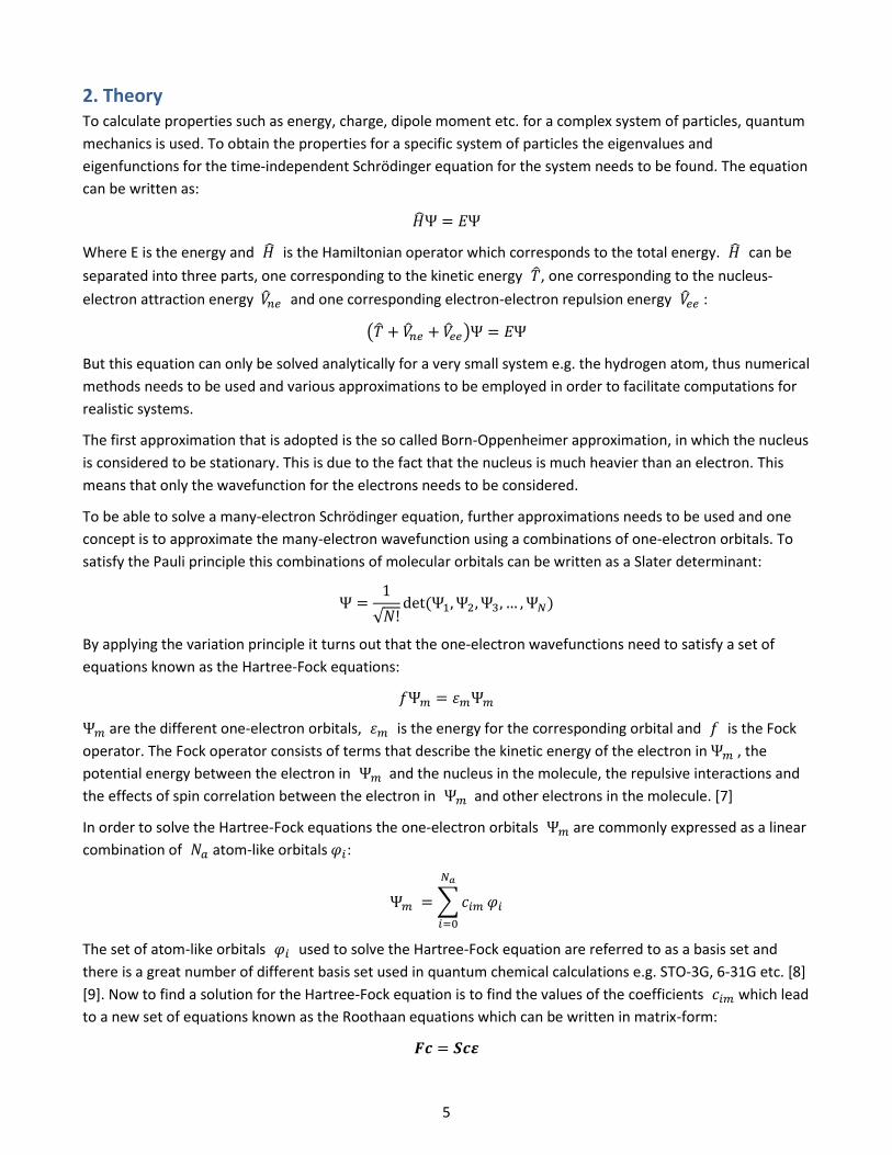
2. Theory To calculate properties such as energy, charge, dipole moment etc. for a complex system of particles, quantum
mechanics is used. To obtain the properties for a specific system of particles the eigenvalues and
eigenfunctions for the time-independent Schrödinger equation for the system needs to be found. The equation
can be written as:
Where E is the energy and is the Hamiltonian operator which corresponds to the total energy. can be
separated into three parts, one corresponding to the kinetic energy , one corresponding to the nucleus-
electron attraction energy and one corresponding electron-electron repulsion energy :
( )
But this equation can only be solved analytically for a very small system e.g. the hydrogen atom, thus numerical
methods needs to be used and various approximations to be employed in order to facilitate computations for
realistic systems.
The first approximation that is adopted is the so called Born-Oppenheimer approximation, in which the nucleus
is considered to be stationary. This is due to the fact that the nucleus is much heavier than an electron. This
means that only the wavefunction for the electrons needs to be considered.
To be able to solve a many-electron Schrödinger equation, further approximations needs to be used and one
concept is to approximate the many-electron wavefunction using a combinations of one-electron orbitals. To
satisfy the Pauli principle this combinations of molecular orbitals can be written as a Slater determinant:
√
By applying the variation principle it turns out that the one-electron wavefunctions need to satisfy a set of
equations known as the Hartree-Fock equations:
are the different one-electron orbitals, is the energy for the corresponding orbital and is the Fock
operator. The Fock operator consists of terms that describe the kinetic energy of the electron in , the
potential energy between the electron in and the nucleus in the molecule, the repulsive interactions and
the effects of spin correlation between the electron in and other electrons in the molecule. [7]
In order to solve the Hartree-Fock equations the one-electron orbitals are commonly expressed as a linear
combination of atom-like orbitals :
∑
The set of atom-like orbitals used to solve the Hartree-Fock equation are referred to as a basis set and
there is a great number of different basis set used in quantum chemical calculations e.g. STO-3G, 6-31G etc. [8]
[9]. Now to find a solution for the Hartree-Fock equation is to find the values of the coefficients which lead
to a new set of equations known as the Roothaan equations which can be written in matrix-form:
6
where is the Fock matrix, is a matrix built up by the coefficients , is a matrix consisting of overlap
integrals and is formed from the molecular orbital energies .
An alternative electronic structure method to the Hartree-Fock procedure is the Density Functional Theory
(DFT), the difference is that the electron density rather than the wave function is the central concept. The
electron density is a function of position and the energy for the system is a function of the electron
density ( ), in other words the energy is a functional, i.e. a function of a function, hence the name
Density Functional Theory.
The electron density can be written as a sum over the occupied orbitals and to obtain the electron density
and the set of orbitals one solves the Kohn-Sham equations. [7]
Electronic structure calculation methods used by quantum-chemistry programs are usually based on Hartree-
Fock or DFT or often a hybrid of the two e.g. B3LYP [10].
3. Computational details In this work the interactions between SiH2 and a 4H-SiC (0001) surface and SiCl2 and a 4H-SiC (0001) surface
were simulated and compared since the 4H-SiC (0001) surface is the growth surface in the CVD process [2]. The
SiC-surface was modelled by a cluster containing a limited amount of atoms. These clusters are constructed
using the crystal SiC structure with space group P63mc and by the aid of the molecular modelling program
Cerius 2 [11].The lattice parameters (in angstrom) used were a=3.08 and c=10.08[12]. Both hydrogen
terminated clusters and non-terminated clusters in different sizes, ranging from 26 to 400 atoms, were
constructed (see appendix A). The geometries of the clusters were obtained from geometry-optimizations to
find the local energy-minimum structures. All electronic structure and geometrical information was computed
using Gaussian 03 [13].
The calculation methods and basis sets used were the B3LYP [10] hybrid density functional with a double-zeta
basis set (DZ) [14][15] or with a 6-31G(d,p) basis set [9]. For investigating the smaller molecules SiH2 and SiCl2
the additional methods QCISD(T) [16], MP2 [17], and MP4 [18], and the basis set 6-311++G(2df,2pd) [19] were
also used.
To calculate the band gaps for the different clusters the energy difference between the lowest unoccupied
molecular orbital (LUMO) and the highest occupied molecular orbital (HOMO) was calculated. This can be
compared to previous work [20].
The cluster used in the molecule-cluster interaction simulations was the H60Si33C33 cluster (see appendix A). This
cluster is large enough to represent a surface with inner surface atoms and small enough to allow for
simulations within a reasonable time. Since it is silicon-based molecules interacting with a carbon surface that
are to be simulated, the surface with carbon atoms as the outermost atoms (except the hydrogen atoms) is
used as the interacting surface. Then one, two or three hydrogen atoms at the carbon surface were replaced in
different ways by different number of silicon-based molecules. The initial silicon-based atom positions were
chosen using well-educated guesses. This was followed by a geometry-optimization where all atoms were
allowed to move. The electronic energies and the Gibbs free energy were calculated for the different
molecules, clusters and molecule-cluster structures. The pressure used when calculating the Gibbs free energy
at reactor pressure for the different molecules and structures can be seen in table 2. These pressures are based
on the molar fraction of the various molecules and the reactor pressure in the CVD process [2]. The
7
temperature used for calculating the Gibbs free energy was 1870 K which represents the temperature usually
used in CVD.
Table 2. Pressure for different molecules and cluster, a also includes all clusters with molecules attached to them.
Structure Pressure [atmospheres]
SiC clustersa 1 H2 0.1 SiCl2 0.0004 SiH2 0.0004 HCl 0.0016 Cl2 0.00005
Visualizations of clusters and molecules were done using Molekel [21] and Moviemol [22]. Molden[23] were
also used when creating molecules and editing clusters. The display of data where made using MATLAB[24].
4. Results and Discussion
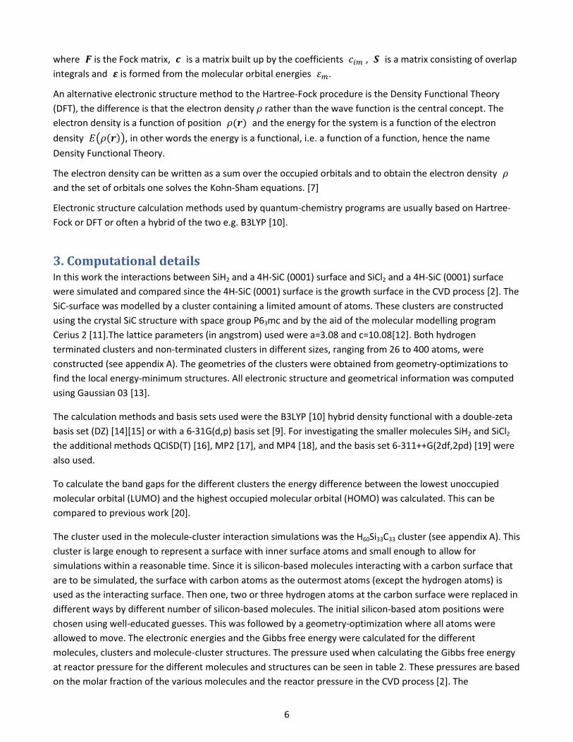
4.1. The SiH2 and SiCl2 molecules
The influence on the molecular energy from the spin multiplicity for SiH2 and SiCl2 where investigated, see table
3 and table 4. Since the energy of the singlet state is seen to be lower than the energy of the triplet state for
both molecules the conclusion is that the singlet spin state is preferable for both SiH2 and SiCl2. For SiCl2 it
agrees with earlier investigations [25]. Thus the energy and geometry corresponding to the singlet spin state
for the two molecules where used subsequently.
Table 3. The energy end geometries for the SiH2 molecule using different methods and basis sets.
SiH2
Method Basis set α [degrees] r [angstrom] ΔE [kJ mol-1]
(Etriplet - Esinglet) Singlet Triplet Singlet Triplet
B3LYP DZ 91.2° 118.7° 1.559 1.503 72
6-311++G(2df,2pd) 91.6° 118.6° 1.523 1.485 85
MP2 DZ 93.0° 118.9° 1.552 1.496 5
6-311++G(2df,2pd) 92.2° 118.2° 1.511 1.473 67
MP4 DZ 92.7° 118.9° 1.566 1.507 40
6-311++G(2df,2pd) 92.2° 118.5° 1.517 1.478 81
QCISD(T) DZ 92.7° 118.8° 1.575 1.510 4
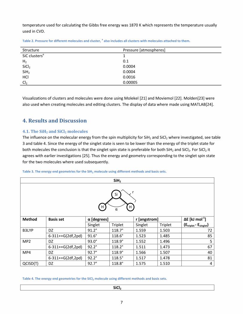
Table 4. The energy end geometries for the SiCl2 molecule using different methods and basis sets.
SiCl2
H
r
α
Si
H
8
Method Basis set α [degrees] r [angstrom] ΔE [kJ mol-1]
(Etriplet - Esinglet) Singlet Triplet Singlet Triplet
B3LYP
DZ 101.8° 120.4° 2.238 2.218 221
6-311++G(2df,2pd) 101.8° 118.6° 2.099 2.068 223
MP2
DZ 101.6° 119.0° 2.240 2.199 149
6-311++G(2df,2pd) 101.3° 118.6° 2.078 2.048 212
MP4
DZ 101.7° 119.3° 2.256 2.214 201
6-311++G(2df,2pd) 101.6° 117.8° 2.085 2.055 225
QCISD(T) DZ 101.6° 119.3° 2.255 2.219 207
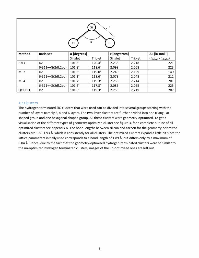
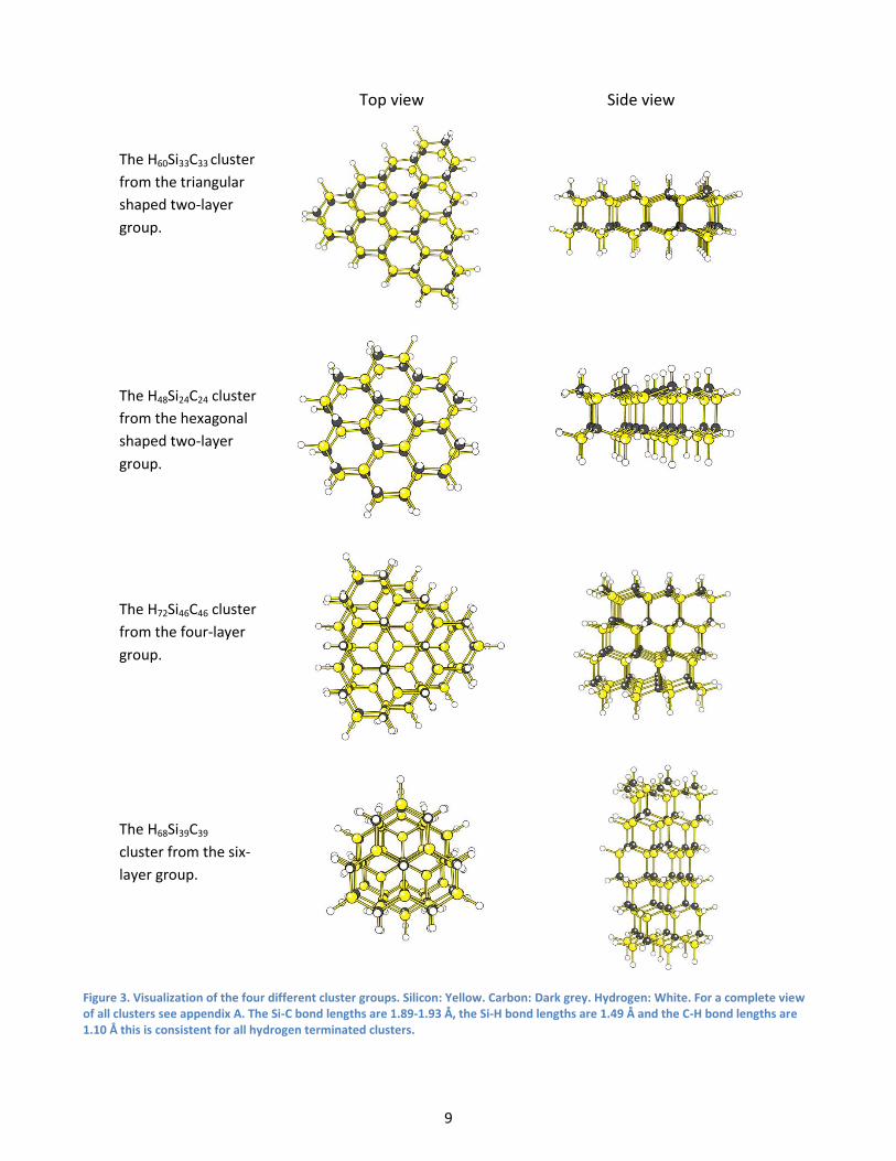
4.2 Clusters
The hydrogen terminated SiC-clusters that were used can be divided into several groups starting with the
number of layers namely 2, 4 and 6 layers. The two-layer clusters are further divided into one triangular-
shaped group and one hexagonal-shaped group. All these clusters were geometry-optimized. To get a
visualisation of the different types of geometry-optimized cluster see figure 3, for a complete outline of all
optimized clusters see appendix A. The bond-lengths between silicon and carbon for the geometry-optimized
clusters are 1.89-1.93 Å, which is consistently for all clusters. The optimized clusters expand a little bit since the
lattice parameters initially used corresponds to a bond length of 1.89 Å, but differs only by a maximum of
0.04 Å. Hence, due to the fact that the geometry-optimized hydrogen-terminated clusters were so similar to
the un-optimized hydrogen terminated clusters, images of the un-optimized ones are left out.
r
α Cl Cl
Si
9
Figure 3. Visualization of the four different cluster groups. Silicon: Yellow. Carbon: Dark grey. Hydrogen: White. For a complete view of all clusters see appendix A. The Si-C bond lengths are 1.89-1.93 Å, the Si-H bond lengths are 1.49 Å and the C-H bond lengths are 1.10 Å this is consistent for all hydrogen terminated clusters.
Top view Side view
The H60Si33C33 cluster
from the triangular
shaped two-layer
group.
The H48Si24C24 cluster
from the hexagonal
shaped two-layer
group.
The H72Si46C46 cluster
from the four-layer
group.
The H68Si39C39
cluster from the six-
layer group.
10
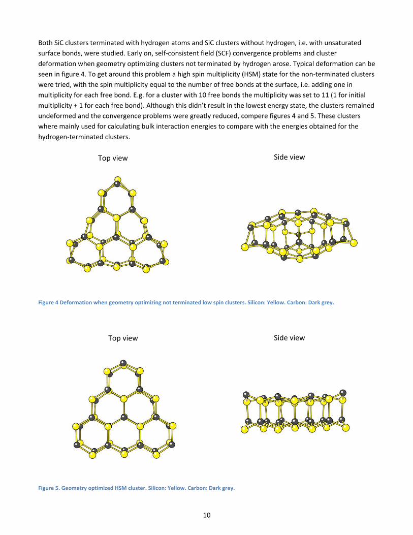
Both SiC clusters terminated with hydrogen atoms and SiC clusters without hydrogen, i.e. with unsaturated
surface bonds, were studied. Early on, self-consistent field (SCF) convergence problems and cluster
deformation when geometry optimizing clusters not terminated by hydrogen arose. Typical deformation can be
seen in figure 4. To get around this problem a high spin multiplicity (HSM) state for the non-terminated clusters
were tried, with the spin multiplicity equal to the number of free bonds at the surface, i.e. adding one in
multiplicity for each free bond. E.g. for a cluster with 10 free bonds the multiplicity was set to 11 (1 for initial
multiplicity + 1 for each free bond). Although this didn’t result in the lowest energy state, the clusters remained
undeformed and the convergence problems were greatly reduced, compere figures 4 and 5. These clusters
where mainly used for calculating bulk interaction energies to compare with the energies obtained for the
hydrogen-terminated clusters.
Figure 4 Deformation when geometry optimizing not terminated low spin clusters. Silicon: Yellow. Carbon: Dark grey.
Figure 5. Geometry optimized HSM cluster. Silicon: Yellow. Carbon: Dark grey.
Top view Side view
Top view Side view

11
4.3. Cluster energies
The interaction energy per SiC unit for the clusters without hydrogen, i.e. the HSM clusters, was calculated
using the formula:
For the hydrogen terminated clusters the formula used is:
where is the total electronic energy for the cluster, and is the electronic energy of a free silicon
and carbon atom, is the number of SiC units and m is the number of hydrogen atoms. is the electronic
energy corresponding to a bonded hydrogen atom and was calculated as the energy difference between a fully
hydrogen terminated cluster and a cluster with one hydrogen atom removed, averaging over different
hydrogen atoms.
As can been seen in figure 6, the cluster energy per SiC unit decreases with larger clusters, and the result is in
fair agreement between the hydrogen terminated cluster and the HSM clusters. This means that a larger
cluster is preferable and therefore crystal growth is anticipated. The linear relation between the cluster energy
per SiC unit and SiC unit raised to minus one third can be shown by a smal calculation, if presuming:
where is cluster energy and are constants, is cluster area and is the volume of the cluster.
Figure 6. Interaction energy for different cluster. On the y-axis the interaction energy per SiC units are displayed in kJ mol-1
. On the x-axis the number of SiC units raised to minus one third is displayed which means larger cluster to the left. The blue marks and line corresponds to the data points and calculated linear fit for the hydrogen-terminated cluster and the red marks and line corresponds to the data points and calculated linear fit for the HSM clusters.
0.2 0.25 0.3 0.35 0.4 0.45-1550
-1500
-1450
-1400
-1350
-1300
-1250
n-1/3
Clu
ste
r energ
y (
E/n
) [k
J m
ol-1
]
Two layers triagonal shape
Two layers round shape
Four layers
Six layers
Linear trend
Two layers triagonal shape
Two layers round shape
Four layers
Six layers
Linear trend

12
4.4. Band gaps
The band gaps were calculated as the difference between the HOMO and LUMO energies for different clusters.
As can be seen in figure 7 the band gap is large for the small clusters but decreases with increased cluster size
and gets closer to the experimental value of 3.2 eV. This is expected due to the quantum confinement effect,
the energy gaps will increase and in particular the band gap will increase with decreasing cluster size. To get a
linear relation between the band gap and cluster size the band gap is plotted against the number of SiC units
raised to minus one third, see figure 8, this relation is found empirically. If extrapolated to zero the expected
band gap for an infinitely large cluster becomes 3.75 eV which still is too large.
Figure 7. Band gap plotted against cluster size (number of SiC units, n, in the clusters). Here the clusters are divided into groups, where the blue curve corresopnds to the triangleshaped clusters, the green curve corresponds to the roundshaped clusters, the red curve represent the four layer clusters and the magenta colored curve represent the six layer clusters, see apendix A.
10 20 30 40 50 60 70 80 90 1005.2
5.4
5.6
5.8
6
6.2
6.4
6.6
6.8
7
n
Bandgap [
eV
]
Two layers triagonal shape
Two layers round shape
Four layers
Six layers
13
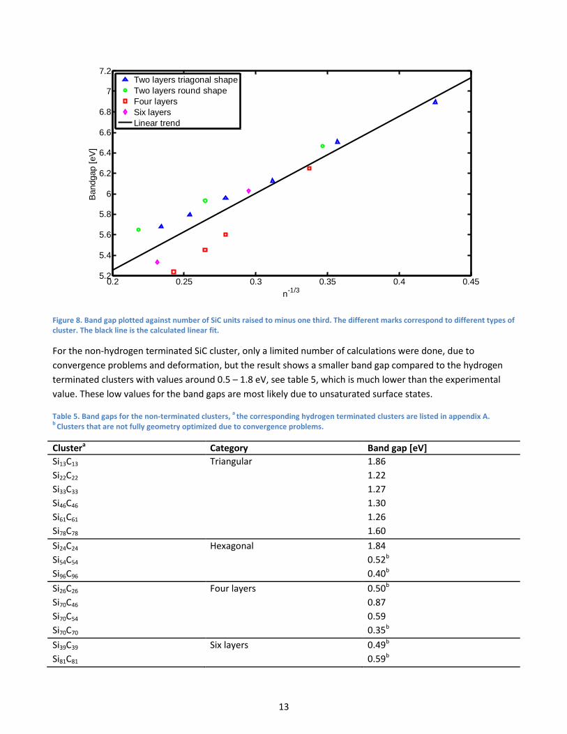
Figure 8. Band gap plotted against number of SiC units raised to minus one third. The different marks correspond to different types of cluster. The black line is the calculated linear fit.
For the non-hydrogen terminated SiC cluster, only a limited number of calculations were done, due to
convergence problems and deformation, but the result shows a smaller band gap compared to the hydrogen
terminated clusters with values around 0.5 – 1.8 eV, see table 5, which is much lower than the experimental
value. These low values for the band gaps are most likely due to unsaturated surface states.
Table 5. Band gaps for the non-terminated clusters, a
the corresponding hydrogen terminated clusters are listed in appendix A. b
Clusters that are not fully geometry optimized due to convergence problems.
Clustera Category Band gap [eV]
Si13C13 Triangular 1.86
Si22C22 1.22
Si33C33 1.27
Si46C46 1.30
Si61C61 1.26
Si78C78 1.60
Si24C24 Hexagonal 1.84
Si54C54 0.52b
Si96C96 0.40b
Si26C26 Four layers 0.50b
Si70C46 0.87
Si70C54 0.59
Si70C70 0.35b
Si39C39 Six layers 0.49b
Si81C81 0.59b
0.2 0.25 0.3 0.35 0.4 0.455.2
5.4
5.6
5.8
6
6.2
6.4
6.6
6.8
7
7.2
n-1/3
Bandgap [
eV
]
Two layers triagonal shape
Two layers round shape
Four layers
Six layers
Linear trend
14
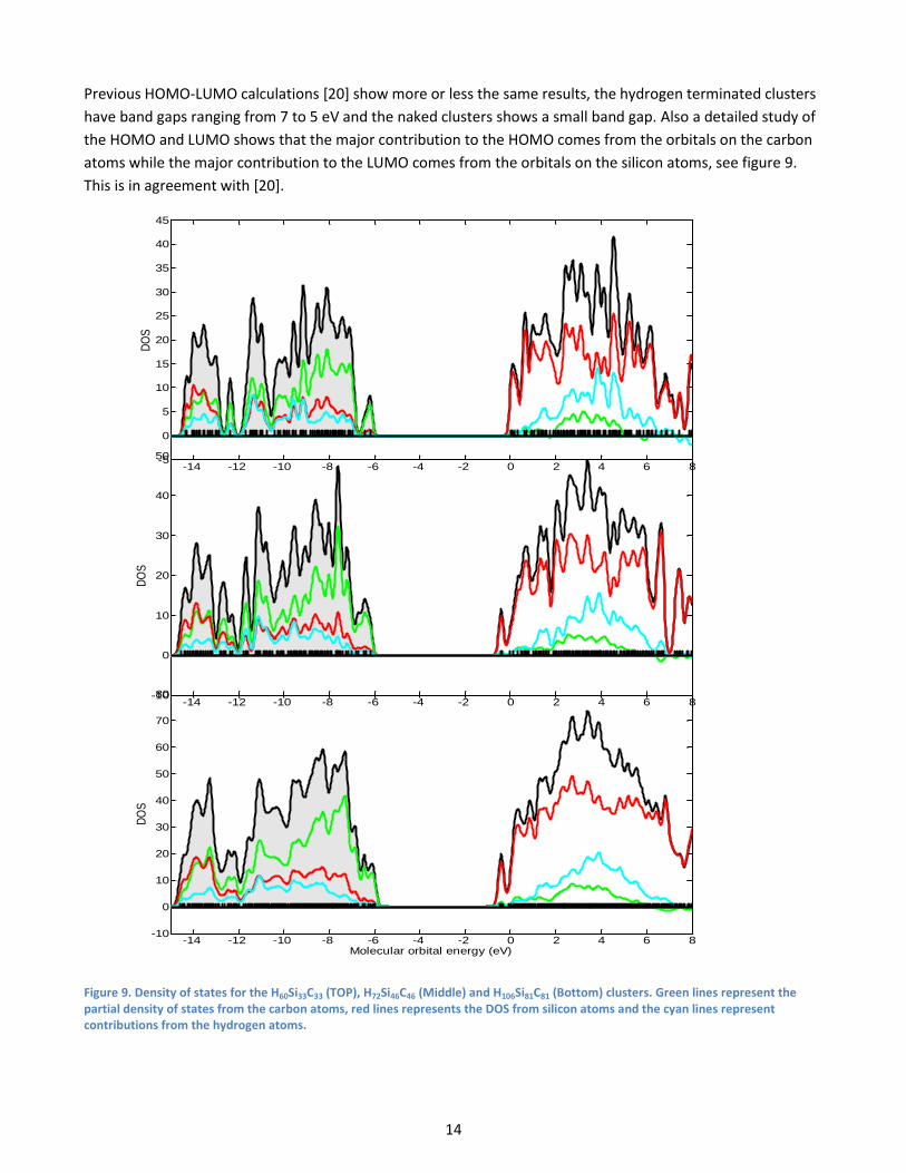
Previous HOMO-LUMO calculations [20] show more or less the same results, the hydrogen terminated clusters
have band gaps ranging from 7 to 5 eV and the naked clusters shows a small band gap. Also a detailed study of
the HOMO and LUMO shows that the major contribution to the HOMO comes from the orbitals on the carbon
atoms while the major contribution to the LUMO comes from the orbitals on the silicon atoms, see figure 9.
This is in agreement with [20].
Figure 9. Density of states for the H60Si33C33 (TOP), H72Si46C46 (Middle) and H106Si81C81 (Bottom) clusters. Green lines represent the partial density of states from the carbon atoms, red lines represents the DOS from silicon atoms and the cyan lines represent contributions from the hydrogen atoms.
-14 -12 -10 -8 -6 -4 -2 0 2 4 6 8-10
0
10
20
30
40
50
60
70
80
Molecular orbital energy (eV)
DO
S
-14 -12 -10 -8 -6 -4 -2 0 2 4 6 8-10
0
10
20
30
40
50
DO
S
-14 -12 -10 -8 -6 -4 -2 0 2 4 6 8-5
0
5
10
15
20
25
30
35
40
45
DO
S
15
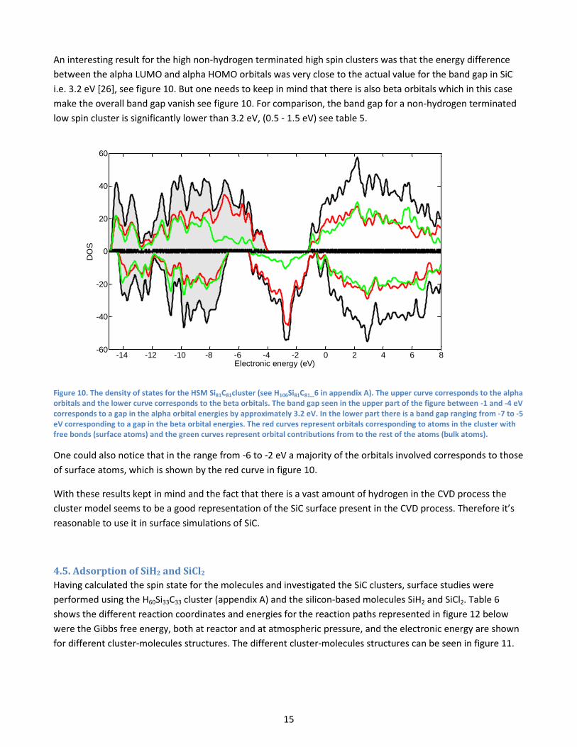
An interesting result for the high non-hydrogen terminated high spin clusters was that the energy difference
between the alpha LUMO and alpha HOMO orbitals was very close to the actual value for the band gap in SiC
i.e. 3.2 eV [26], see figure 10. But one needs to keep in mind that there is also beta orbitals which in this case
make the overall band gap vanish see figure 10. For comparison, the band gap for a non-hydrogen terminated
low spin cluster is significantly lower than 3.2 eV, (0.5 - 1.5 eV) see table 5.
Figure 10. The density of states for the HSM Si81C81cluster (see H106Si81C81_6 in appendix A). The upper curve corresponds to the alpha orbitals and the lower curve corresponds to the beta orbitals. The band gap seen in the upper part of the figure between -1 and -4 eV corresponds to a gap in the alpha orbital energies by approximately 3.2 eV. In the lower part there is a band gap ranging from -7 to -5 eV corresponding to a gap in the beta orbital energies. The red curves represent orbitals corresponding to atoms in the cluster with free bonds (surface atoms) and the green curves represent orbital contributions from to the rest of the atoms (bulk atoms).
One could also notice that in the range from -6 to -2 eV a majority of the orbitals involved corresponds to those
of surface atoms, which is shown by the red curve in figure 10.
With these results kept in mind and the fact that there is a vast amount of hydrogen in the CVD process the
cluster model seems to be a good representation of the SiC surface present in the CVD process. Therefore it’s
reasonable to use it in surface simulations of SiC.
4.5. Adsorption of SiH2 and SiCl2
Having calculated the spin state for the molecules and investigated the SiC clusters, surface studies were
performed using the H60Si33C33 cluster (appendix A) and the silicon-based molecules SiH2 and SiCl2. Table 6
shows the different reaction coordinates and energies for the reaction paths represented in figure 12 below
were the Gibbs free energy, both at reactor and at atmospheric pressure, and the electronic energy are shown
for different cluster-molecules structures. The different cluster-molecules structures can be seen in figure 11.
-14 -12 -10 -8 -6 -4 -2 0 2 4 6 8-60
-40
-20
0
20
40
60
Electronic energy (eV)
DO
S
16
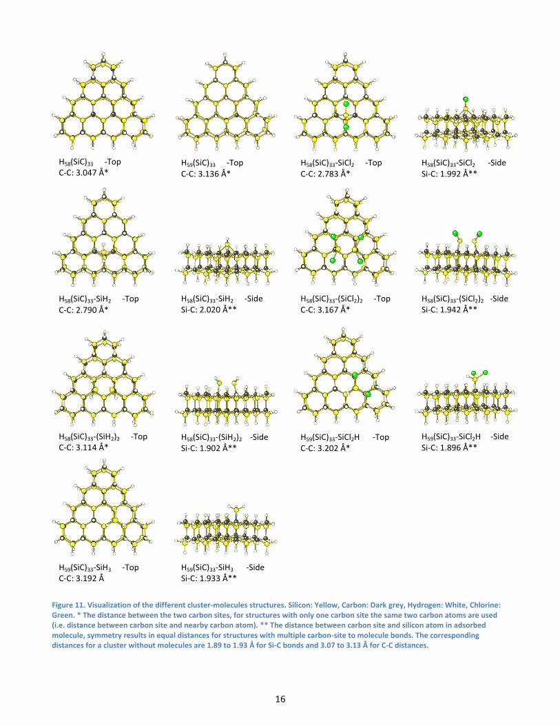
Figure 11. Visualization of the different cluster-molecules structures. Silicon: Yellow, Carbon: Dark grey, Hydrogen: White, Chlorine: Green. * The distance between the two carbon sites, for structures with only one carbon site the same two carbon atoms are used (i.e. distance between carbon site and nearby carbon atom). ** The distance between carbon site and silicon atom in adsorbed molecule, symmetry results in equal distances for structures with multiple carbon-site to molecule bonds. The corresponding distances for a cluster without molecules are 1.89 to 1.93 Å for Si-C bonds and 3.07 to 3.13 Å for C-C distances.
H58(SiC)33 -Top C-C: 3.047 Å*
H59(SiC)33 -Top C-C: 3.136 Å*
H58(SiC)33-SiCl2 -Top C-C: 2.783 Å*
H58(SiC)33-SiCl2 -Side Si-C: 1.992 Å**
H58(SiC)33-SiH2 -Top C-C: 2.790 Å*
H58(SiC)33-SiH2 -Side Si-C: 2.020 Å**
H58(SiC)33-(SiCl2)2 -Top C-C: 3.167 Å*
H58(SiC)33-(SiCl2)2 -Side Si-C: 1.942 Å**
H58(SiC)33-(SiH2)2 -Top C-C: 3.114 Å*
H58(SiC)33-(SiH2)2 -Side Si-C: 1.902 Å**
H59(SiC)33-SiCl2H -Top C-C: 3.202 Å*
H59(SiC)33-SiCl2H -Side Si-C: 1.896 Å**
H59(SiC)33-SiH3 -Top C-C: 3.192 Å
H59(SiC)33-SiH3 -Side Si-C: 1.933 Å**

17
Table 6. a
See H60Si33C33 appendix A. b c d e f g h i
See figure 11 for visualisations of the structures.
Reaction Coordinate Structure ΔE [kJ mol-1] ΔG [kJ mol-1] (reactor pressure)
ΔG [kJ mol-1] (at 1 atm)
H60(SiC)33 a + H2 + SiCl2 0 0 0
H58(SiC)33b + 2H2 + SiCl2 395 155 190
H58(SiC)33-SiCl2c +2H2 105 273 187
H58(SiC)33-SiH2d + Cl2 + H2 414 430 463
H58(SiC)33-SiH2 + 2HCl 207 196 238
H60(SiC)33 + 3H2 + 2SiCl2 0 0 0
H58(SiC)33 + 4H2 + 2SiCl2 395 155 190
H58(SiC)33-(SiCl2)2e +4H2 -184 485 277
H58(SiC)33-(SiH2)2f + 2Cl2 + 2H2 461 798 826
H58(SiC)33-(SiH2)2 + 4HCl 48 327 378
H60(SiC)33 + SiH2 0 0 0
H58(SiC)33 + H2 + SiH2 395 155 190
H58(SiC)33-SiH2 +H2 -14 142 56
H60(SiC)33 + 2SiH2 0 0 0
H58(SiC)33 + H2 + 2SiH2 395 155 190
H58(SiC)33-(SiH2)2 +H2 -395 221 14
H60(SiC)33 + SiH2 0 0 0
H59(SiC)33
g + 1/2H2 + SiH2 86 23 41
H59(SiC)33-SiH3
h -213 222 100
H60(SiC)33 + SiCl2 0 0 0
H59(SiC)33 + 1/2H2 + SiCl2 86 23 41
H59(SiC)33-SiCl2Hi -106 357 235
18
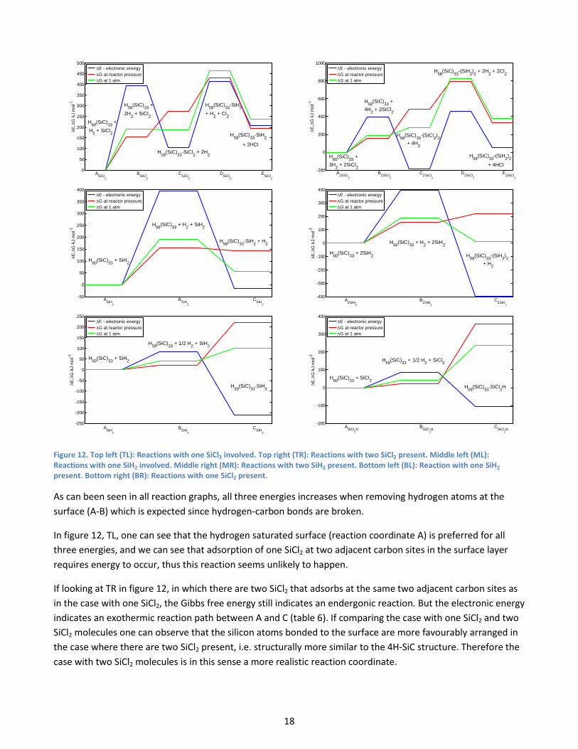
Figure 12. Top left (TL): Reactions with one SiCl2 involved. Top right (TR): Reactions with two SiCl2 present. Middle left (ML): Reactions with one SiH2 involved. Middle right (MR): Reactions with two SiH2 present. Bottom left (BL): Reaction with one SiH2 present. Bottom right (BR): Reactions with one SiCl2 present.
As can been seen in all reaction graphs, all three energies increases when removing hydrogen atoms at the
surface (A-B) which is expected since hydrogen-carbon bonds are broken.
In figure 12, TL, one can see that the hydrogen saturated surface (reaction coordinate A) is preferred for all
three energies, and we can see that adsorption of one SiCl2 at two adjacent carbon sites in the surface layer
requires energy to occur, thus this reaction seems unlikely to happen.
If looking at TR in figure 12, in which there are two SiCl2 that adsorbs at the same two adjacent carbon sites as
in the case with one SiCl2, the Gibbs free energy still indicates an endergonic reaction. But the electronic energy
indicates an exothermic reaction path between A and C (table 6). If comparing the case with one SiCl2 and two
SiCl2 molecules one can observe that the silicon atoms bonded to the surface are more favourably arranged in
the case where there are two SiCl2 present, i.e. structurally more similar to the 4H-SiC structure. Therefore the
case with two SiCl2 molecules is in this sense a more realistic reaction coordinate.
0
50
100
150
200
250
300
350
400
450
500
E
,G
kJ m
ol-1
H60
(SiC)33
+
H2 + SiCl
2
H58
(SiC)33
+
2H2 + SiCl
2
H58
(SiC)33
-SiCl2 + 2H
2
H58
(SiC)33
-SiH2
+ H2 + Cl
2
H58
(SiC)33
-SiH2
+ 2HCl
ASiCl
2
BSiCl
2
CSiCl
2
DSiCl
2
ESiCl
2
E - electronic energy
G at reactor pressure
G at 1 atm
-200
0
200
400
600
800
1000
E
,G
kJ m
ol-1
H60
(SiC)33
+
3H2 + 2SiCl
2
H58
(SiC)33
+
4H2 + 2SiCl
2
H58
(SiC)33
-(SiCl2)2
+ 4H2
H58
(SiC)33
-(SiH2)2 + 2H
2 + 2Cl
2
H58
(SiC)33
-(SiH2)2
+ 4HCl
A2SiCl
2
B2SiCl
2
C2SiCl
2
D2SiCl
2
E2SiCl
2
E - electronic energy
G at reactor pressure
G at 1 atm
-50
0
50
100
150
200
250
300
350
400
E
,G
kJ m
ol-1
H60
(SiC)33
+ SiH2
H58
(SiC)33
+ H2 + SiH
2
H58
(SiC)33
-SiH2 + H
2
ASiH
2
BSiH
2
CSiH
2
E - electronic energy
G at reactor pressure
G at 1 atm
-400
-300
-200
-100
0
100
200
300
400
E
,G
kJ m
ol-1
H60
(SiC)33
+ 2SiH2
H58
(SiC)33
+ H2 + 2SiH
2
H58
(SiC)33
-(SiH2)2
+ H2
A2SiH
2
B2SiH
2
C2SiH
2
E - electronic energy
G at reactor pressure
G at 1 atm
-250
-200
-150
-100
-50
0
50
100
150
200
250
E
,G
kJ m
ol-1
H60
(SiC)33
+ SiH2
H59
(SiC)33
+ 1/2 H2 + SiH
2
H59
(SiC)33
-SiH3
ASiH
3
BSiH
3
CSiH
3
E - electronic energy
G at reactor pressure
G at 1 atm
-200
-100
0
100
200
300
400
E,
G k
J m
ol-1
H60
(SiC)33
+ SiCl2
H59
(SiC)33
+ 1/2 H2 + SiCl
2
H59
(SiC)33
-SiCl2H
ASiCl
2H
BSiCl
2H
CSiCl
2H
E - electronic energy
G at reactor pressure
G at 1 atm
19
In figure 12, ML, the reaction path of one SiH2 adsorbed at two adjacent carbon sites is shown and as can be
seen the Gibbs free energy at the two different pressure configurations indicates an endergonic reaction but
the electronic energy shows a small fall in energy. There are similarities between the adsorption of one SiH2
and SiCl2 at two carbon sites, but for SiH2 the adsorption seems stronger since the change in energy between A
and C is approximately 100 kJ mol-1 lower (decreases more or increases less) for SiH2 compared to SiCl2.
The reaction path for adsorption of two SiH2 at the two adjacent carbon sites is shown in figure 12, MR. The
Gibbs free energy indicates an endergonic reaction here as well. But the electronic energy exhibits a big fall in
energy between A and C. If one compare this result with the SiCl2 case, then one observes the same difference
here as in the cases with only one molecule, and that is that SiH2 seems to adsorb stronger to the surface since
the energy change between A and C is approximately 200 kJ mol-1 lower for the two SiH2 molecules compared
to the two SiCl2 molecules.
In the BL and the BR in figure 12 only one hydrogen is removed. In the BL it is replaced by a SiH2 with the
removed hydrogen atom attached to it, making it a SiH3 molecule binding at the free carbon site. In BR the
hydrogen atom is replaced with a SiCl2 molecule with the additional hydrogen atom attached to it, making it a
SiCl2H molecule binding at the free carbon site. If comparing these reactions with the previous, we obtain a
similar result. The energy decreases approximately 100 kJ mol-1 more between A and C for the SiH2 molecule
compared to the SiCl2 molecule. This configuration also gives the strongest adsorption energy per molecule
with 213 kJ mol-1 for the SiH2 and 106 kJ mol-1for the SiCl2, see table 6.
So if considering these three cases the adsorption energy seems to be approximately 100 kJ mol-1 stronger per
molecule for SiH2 compared to SiCl2 and the adsorption energy should be close to 213 kJ mol-1 for the SiH2
molecule and 106 kJ mol-1for the SiCl2 molecule.
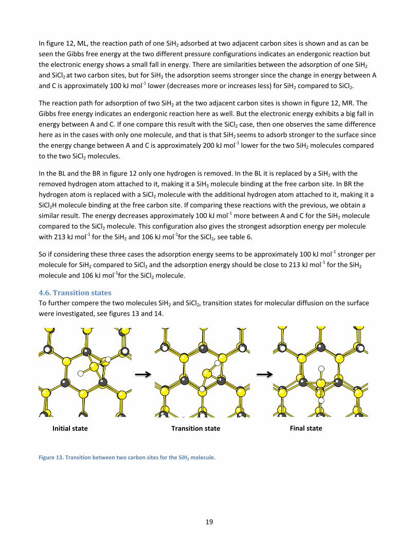
4.6. Transition states
To further compere the two molecules SiH2 and SiCl2, transition states for molecular diffusion on the surface
were investigated, see figures 13 and 14.
Figure 13. Transition between two carbon sites for the SiH2 molecule.
Initial state Transition state Final state

20
Figure 14. Transition between two carbon sites for the SiH2 molecule.
The activation energy required for the migration of the SiH2 molecule was 87 kJ mol-1.The same transition for
SiCl2 involves an additional minimum state between the state before and the state after as can be seen in
figure 17. Nevertheless the activation energy required for the migration of the SiCl2 molecule is in this case 4 kJ
mol-1, i.e. the higher of the two activation energies required for the two different transition states. As can be
seen, the activation energy required for SiH2 is significantly higher than the activation energy required for SiCl2.
This means that the SiCl2 molecule more easily can diffuse on the surface. This is beneficial for producing a
smooth surface and avoiding island growth, i.e. local areas where the number of layers is larger than
elsewhere.
5. Conclusions There are two primary conclusions to be drawn from this research. First, SiH2 adsorbs more strongly to the
surface (around 213 kJ mol-1) than SiCl2 (around 106 kJ mol-1) which suggest that the growth rate should be
faster with SiH2 molecules if we consider a case where there are the same amount of SiH2 and SiCl2 molecules
present in the gas phase. But without chloride present in the process a too great concentration of silicon in the
gas phase leads to defects to be formed on the surface, which makes the product useless.
Secondly, the activation energy for migration on the surface for SiCl2 molecule is only 4 kJ mol-1 which is clearly
lower than the activation energy for the SiH2 molecule (87 kJ mol-1). This implies that SiCl2 can diffuse more
Initial state Transition Local minimum
Transition Final state

21
easily on the surface compared to the SiH2. This suggests that the molecules on the surface more easily can
move to the globally lowest energy state. This would mean that the epitaxial layer growth with chloride
involved has lesser risk for structural impurities and thereby should produce a better surface. This might be an
additional reason, aside from the dissolvent of silicon droplet in the gas phase, to why having chloride present
in the system allows for a greater concentration of silicon in the gas phase and thereby a faster growth rate.
One should keep in mind that this is just a few reaction paths that have yet been investigated and a limited
amount of adsorption studies performed as well.
6. Future work There are a lot of things to consider in future works in this area and here follows a few interesting points.
Tests should be performed using a larger cluster (at least four layers) to rule out any influences the
other side of the cluster could have had on the molecules.
Additional arrangement of the molecules on the surface should be investigated to ensure good
adsorption values.
More transition states and reaction paths should be studied in order to better understand how the
molecules diffuse on the surface.
Other halogens beside chlorine would also be interesting to simulate, perhaps there is a theoretically
more promising candidate besides chloride.
To really simulate the growth process one should also consider the carbon-based molecules present.
These molecules need also to be considered if one wants to fully understand the role chlorine plays in
the growth process.

22
References [1] H. Pedersen, Chloride-based Silicon Carbide CVD, Diss Thesis no. 1225, Linköping University, Linköping,
Sweden (2008).
[2] H. Pedersen, S. Leone, O. Kordina, A. Henry, S. Nishizawa, Y. Koshka, and E. Janzén, Chem. Rev., 2012, v.
112 , p 2434.
[3] G. Aylward, T. Findlay, SI Chemical Data, 4th ed. John Wiley & Sons, Australia, 1998, p 115.
[4] G. Valente, C. Cavallotti, M. Masi, C. Carrà, J. Cryst. Growth, 2001, v. 230, p. 247.
[5] S. Nigam, H. J. Chung, A. Y. Polyakov, M. A. Fanton, B. E. Weiland, D. W. Snyder, M. Skowronski, J. Cryst.
Growth, 2005, v. 284, p. 112.
[6] A. Veneroni, F. Omarini, M. Masi, Cryst. Res. Technol., 2005, v. 40, p. 967.
[7] P. Atkins, J. de Paula, Atkins’ Physical Chemistry 9th edition, p. 401.
[8] W. J. Hehre, R. F. Stewart, and J. A. Pople, J. Chem. Phys., 1969, v. 51, p. 265.
[9] W. J. Hehre, R. Ditchfield, and J. A. Pople, J. Chem. Phys., 1972, v. 56, p. 2257.
[10] A.D. Becke, J. Chem. Phys., 1993, v. 98, p. 5648.
[11] Cerius2 4.8 Accelrys, Inc., San Diego, CA, 2003.
[12] A.Ellison, Silicon Carbide Growth by High Temperature CVD Techniques, Diss. Thesis no. 599, Linköping
University, Linköping, Sweden (1999).
[13] M. J. Frisch, G. W. Trucks, H. B. Schlegel, G. E. Scuseria, M. A. Robb, J. R. Cheeseman, J. A. Montgomery, Jr.,
T. Vreven, K. N. Kudin, J. C. Burant, J. M. Millam, S. S. Iyengar, J. Tomasi, V. Barone, B. Mennucci, M. Cossi, G.
Scalmani, N. Rega, G. A. Petersson, H. Nakatsuji, M. Hada, M. Ehara, K. Toyota, R. Fukuda, J. Hasegawa, M.
Ishida, T. Nakajima, Y. Honda, O. Kitao, H. Nakai, M. Klene, X. Li, J. E. Knox, H. P. Hratchian, J. B. Cross, V.
Bakken, C. Adamo, J. Jaramillo, R. Gomperts, R. E. Stratmann, O. Yazyev, A. J. Austin, R. Cammi, C. Pomelli, J. W.
Ochterski, P. Y. Ayala, K. Morokuma, G. A. Voth, P. Salvador, J. J. Dannenberg, V. G. Zakrzewski, S. Dapprich, A.
D. Daniels, M. C. Strain, O. Farkas, D. K. Malick, A. D. Rabuck, K. Raghavachari, J. B. Foresman, J. V. Ortiz, Q. Cui,
A. G. Baboul, S. Clifford, J. Cioslowski, B. B. Stefanov, G. Liu, A. Liashenko, P. Piskorz, I. Komaromi, R. L. Martin,
D. J. Fox, T. Keith, M. A. Al-Laham, C. Y. Peng, A. Nanayakkara, M. Challacombe, P. M. W. Gill, B. Johnson, W.
Chen, M. W. Wong, C. Gonzalez, and J. A. Pople, Gaussian, Inc., Wallingford CT, 2004.
[14] Y. Bouteiller, C. Mijoule, M. Nizam, J. C. Barthelat, J. P. Daudey, M. Pelissier, B. Silvi, Mol. Phys., 1988, v. 65,
p. 295.
[15] P. Durand, J. C. Barthelat, Theor. Chim. Acta., 1975, v. 38, p. 283.
[16] J. A. Pople, M. Head-Gordon, K. Raghavachari, J. Chem. Phys., 1987, v. 87, p. 5968.
[17] M. Head-Gordon, J. A. Pople, and M. J. Frisch, Chem. Phys. Lett., 1988, v. 153, p. 503.
23
[18] K. Raghavachari and J. A. Pople, Int. J. Quantum Chem., 1978, v. 14, p. 91.
[19] M. J. Frisch, J. A. Pople, and J. S. Binkley, J. Chem. Phys., 1984, v. 80, p. 3265.
[20] Supriya Saha, Pranab Sarkar, Chem. Phys. Lett., 2012, v. 536, p. 118.
[21] MOLEKEL, Version 4.3.linux-mesa, Date: 11.Nov.02 by Stefan Portmann, Copyright © 2002 CSCS/ETHZ.
[22] K. Hermansson and L. Ojamäe, "MOVIEMOL: an easy-to-use molecular display and animation program.
User Manual," Report No. UUIC-B19-500, Institute of Chemistry, Uppsala University (1994).
[23] G.Schaftenaar and J.H. Noordik, "Molden: a pre- and post-processing program for molecular and electronic
structures", J. Comput.-Aided Mol. Design, 2000, v. 14, p. 123.
[24] MATLAB 7.11.0.584, The MathWorks Inc., Natick, MA, 2010.
[25] J. M. Coffin, T. P. Hamilton, P. Pulay, and I. Hargittai, Inorg. Chem., 1989, v. 28, p. 4092.
[26] W. J. Choyke D. R. Hamiltgn, L. Patrick, Phys. Rev., 1964, v. 133, p. A1163.