quantum chaos on a curved surface - diva portal126936/fulltext02.pdf · quantum chaos on a curved...

Department of Physics, Chemistry and Biology

Master’s Thesis

Quantum Chaos On A Curved Surface

John Warna

LiTH-IFM-A-EX-08/2027-SE

Department of Physics, Chemistry and BiologyLinkopings universitet, SE-581 83 Linkoping, Sweden

Master’s ThesisLiTH-IFM-A-EX-08/2027-SE


John Warna

Adviser: Irina Yakimenko

Theoretical Physics

Karl-Fredrik Berggren

Theoretical Physics

Examiner: Irina Yakimenko

Theoretical Physics

Linkoping, 20 November, 2008

Avdelning, Institution

Division, Department

Theoretical PhysicsDepartment of Physics, Chemistry and BiologyLinkopings universitet, SE-581 83 Linkoping, Sweden

Datum

Date

2008-11-20

Sprak

Language

� Svenska/Swedish

� Engelska/English

�

�

Rapporttyp

Report category

� Licentiatavhandling

� Examensarbete

� C-uppsats

� D-uppsats

� Ovrig rapport

�

ISBN

ISRN

Serietitel och serienummer

Title of series, numberingISSN

URL for elektronisk version

Titel

TitleKvantkaos Pa Krokt Yta


Forfattare

AuthorJohn Warna

Sammanfattning

Abstract

The system studied in the thesis is a particle in a two-dimensional box on thesurface of a sphere with constant radius. The different systems have differentradii while the box dimension is kept the same, so the curvature of the surfaceof the box is different for the different systems. In a system with a sphere of alarge radius the surface of the box is almost flat. What happens if the radius isdecreased and the symmetry is broken? Will the system become chaotic if theradius is small enough? There are some properties of the eigenfunctions, thatshow different things depending on whether the system is chaotic or regular. Theamplitude distribution of the probability density, the amplitude distribution ofthe eigenfunction and the probability density look different for chaotic and regularsystems. The main subject of this thesis is to study these distributions.

Nyckelord

KeywordsPut your keywords here

�

—

LiTH-IFM-A-EX-08/2027-SE

—

Abstract

The system studied in the thesis is a particle in a two-dimensional box on thesurface of a sphere with constant radius. The different systems have differentradii while the box dimension is kept the same, so the curvature of the surfaceof the box is different for the different systems. In a system with a sphere of alarge radius the surface of the box is almost flat. What happens if the radius isdecreased and the symmetry is broken? Will the system become chaotic if theradius is small enough? There are some properties of the eigenfunctions, thatshow different things depending on whether the system is chaotic or regular. Theamplitude distribution of the probability density, the amplitude distribution ofthe eigenfunction and the probability density look different for chaotic and regularsystems. The main subject of this thesis is to study these distributions.

v

Acknowledgements

I would like to thank my supervisors Irina Yakimenko and Karl-Fredrik Berggrenfor the subject of the diploma work and for all help and support during the work.I also would like to thank Bjorn Wahlstrand for his patient help, good advice andfor his role as the opponent.

vii

Contents

1 Introduction 1

1.1 The aim of the thesis . . . . . . . . . . . . . . . . . . . . . . . . . . 1

2 Theory 3

2.1 Quantum mechanics . . . . . . . . . . . . . . . . . . . . . . . . . . 3

2.2 Regular systems become chaotic . . . . . . . . . . . . . . . . . . . 3

2.3 Quantum chaos . . . . . . . . . . . . . . . . . . . . . . . . . . . . . 5

3 Method 7

3.1 Finite Difference Method . . . . . . . . . . . . . . . . . . . . . . . 7

3.2 The kinetic energy part of the Hamiltonian matrix . . . . . . . . . 8

3.3 Building the box . . . . . . . . . . . . . . . . . . . . . . . . . . . . 9

4 Test of the method 13

5 Statistical Properties 17

5.1 Distribution of the probability function . . . . . . . . . . . . . . . 17

5.1.1 Results . . . . . . . . . . . . . . . . . . . . . . . . . . . . . 17

5.1.2 Pictures . . . . . . . . . . . . . . . . . . . . . . . . . . . . . 18

5.2 The Porter-Thomas distribution for different eigenfunctions . . . . 23

5.2.1 Results . . . . . . . . . . . . . . . . . . . . . . . . . . . . . 23

5.2.2 Pictures . . . . . . . . . . . . . . . . . . . . . . . . . . . . . 23

5.3 Amplitude distribution of the eigenfunction . . . . . . . . . . . . . 26

5.3.1 Results . . . . . . . . . . . . . . . . . . . . . . . . . . . . . 26

5.3.2 Pictures . . . . . . . . . . . . . . . . . . . . . . . . . . . . . 26

6 Show the curvature 31

7 Limits and tips for the reader 33

7.1 Resolution of the FDM . . . . . . . . . . . . . . . . . . . . . . . . . 33

7.2 Better resolution of the box . . . . . . . . . . . . . . . . . . . . . . 33

7.3 The smallest sphere posible . . . . . . . . . . . . . . . . . . . . . . 33

ix

x Contents

8 Discussion and conclusion 35

8.1 The eigenfunctions ψ and the probability density |ψ|2 . . . . . . . 358.2 Porter-Thomas . . . . . . . . . . . . . . . . . . . . . . . . . . . . . 358.3 Amplitude distribution and Gaussian clock curve . . . . . . . . . . 368.4 Conclusion . . . . . . . . . . . . . . . . . . . . . . . . . . . . . . . 36

Bibliography 37

Chapter 1

Introduction

The Schrodinger equation and the particle in a box-solution [1] are often usedbecause of their simplicity and because real systems, for example microwave bil-liards, can be modelled using this approximation. Two-dimensional quantum bil-liards and microwave billiards are well known systems in the quantum physics.The experiments are of importance and of both theoretical and parctical use inthe quantum chaos field [2]. In this thesis we go from the two-dimensional billiardsinto a new field of quasi-three-dimensional structures. The system studied in hereis a particle in a two-dimensional box on the surface of a sphere. The sphere canhave different radii. The hypothesis is that the system becomes chaotic, if the ra-dius is small enough. The studies discussed are purely theoretical, however, theycould be of interest for manufacturing of chaotic quantum structures.

1.1 The aim of the thesis

A large part of this thesis focuses on the method and how to model the system,which is presented in chapter 3 and 4. In chapter 5, 6 and 7 the results of thecalculations are presented. Chapter 8 contains practical advice for further work.And finally in chapter 9 there are discussions and conclusions.

1

2 Introduction

Chapter 2

Theory

Here follows a short introduction of quantum mechanics and quantum chaos.

2.1 Quantum mechanics

There is no rigorous presentation of quantum mechanics needed in this thesis. Theonly thing needed is the time-independent Schrodinger equation:

− ~2

2m∇2ψ + V ψ = Eψ (2.1)

In the system ”particle in a box” V is zero inside the box and goes to infinityoutside. Therefore Eq. (2.1) can be written as,

− ~2

2m∇2ψ = Eψ (2.2)

where E is the total energy of the particle:

En,m =~

2π2

2me

(n2

a2+m2

b2

)

, (2.3)

where a and b are the sidelengths of the two-dimensional box and n and m arethe two quantum numbers of the system in the x-y-direction respectively. Theeigenfunctions corresponding to eigenvalues are of the form:

ψn,m =

√

1

asin

(nπx

a

)

√

1

bsin

(mπy

b

)

(2.4)

and |ψ|2 is the probability density of the function [1].

2.2 Regular systems become chaotic

In a rectangular system (discussed in section 2.1) the Schrodinger equation isregular or integrable, which means that it is possible to separate the equation into

3

4 Theory

independent equations one for each degree of freedom. It is easy to calculate thecorresponding classical path of the particle in the box. If the system is shapedlike a hockey arena or the symmetry of the system is broken in an another way,it is no longer possible to separate the equation into independent equations. Thesystem is irregular or non-integrable. (see figure 2.1 and 2.2) If the movementof the particle is calculated, the time evolution of the particle’s path will changerapidly with small changes in the initial conditions. The system is now chaotic [3].

0 10 20 30 40 50 60 70 80 900

10

20

30

40

50

60

70

80

90

10 20 30 40 50 60 70 80 90 100

5

10

15

20

25

30

35

40

45

50

Figure 2.1. The system goes from a rectangular grid to a grid shaped like a hockeyarena.

0

20

40

60

80

100

0

20

40

60

80

100−1

−0.8

−0.6

−0.4

−0.2

0

0.2

0.4

0.6

0.8

1

0

20

40

60

80

100

0

20

40

60

80

1000.93

0.94

0.95

0.96

0.97

0.98

0.99

1

Figure 2.2. The system goes from a flat rectangular grid to a grid on a curved surface.

2.3 Quantum chaos 5

2.3 Quantum chaos

Quantum chaos can be shown through the statistical properties of the eigenfunc-tion, amplitude and intensity distributions [4]. A non chaotic wave function showsits nodal pattern as a regular net of intersecting circles and straight lines. In achaotic wave function the nodal lines never intersect [3] and the wave functionis effectively indistinguishable from a superposition of plane waves of fixed wave-vector magnitude with random amplitude, phase and direction. The amplitudedistribution of a chaotic wave follows a Gaussian curve [4],

P (ψ) =1

σ√

2πexp(

−ψ2

2σ2) (2.5)

where σ is the standard deviation,σ =√

∑

ψ ψ2P (ψ). The intensity distribution

follows the Porter-Thomas distribution function [4]:

P (|ψ|2) =1

√

2π|ψ|2exp

(−|ψ|22

)

(2.6)

6 Theory

Chapter 3

Method

To compute the Schrodinger equation Matlab uses matrix multiplication with avector, f:

Af + V f = Eif (3.1)

Ei is the eigenvalue. For a rectangle Ei is En,m, where n and m are quantumnumbers. A and V are the kinetic energy part and the potential energy partof the Hamiltonian matrix. The x-y-plane defined by [0, xend] and [0, yend] andθ − φ− plane defined by [θstart, θend] and [φstart, φend] are divided in grid points,therefore the vector fi,j have indices i and j. The matricies A and V have indicesl and k, where l goes from zero to i× j and k goes from i× j. The maximum ofi represents the points on the x or θ axis and j represents points on y or φ axis.The maximum of i determines the number of rows and j determines the numberof columns in the grid.The kinetic energy part of the Hamiltonian matrix (Al,k) is built using the FiniteDifference Method (FDM). Then Matlab solves the matrix eigenvalue problem,which is a system of equations with one equation for each grid point Eq. (3.1) [5].

3.1 Finite Difference Method

In this method the derivaties each represented at each point as the difference of thevalue of the function in the two (or four in the two-dimensional case) neighbouringgrid points divided by the distance between them [5].For the x-y-grid we have,in x-direction:

δf(x, y)

δx=fi+1,j − fi−1,j

2a(3.2)

δ2f(x, y)

δx2=fi+1,j + fi−1,j − 2fi,j

a2(3.3)

and in y-direction:δf(x, y)

δy=fi,j+1 − fi,j−1

2b(3.4)

7

8 Method

δ2f(x, y)

δy2=fi,j+1 + fi,j−1 − 2fi,j

b2(3.5)

and

∇2f(x, y) =a2fi,j+1 + a2fi,j−1 + b2fi+1,j + b2fi−1,j − 2a2fi,j − 2b2fi,j

a2b2(3.6)

where a and b are the distances between two grid points in x and y directionsrespectively or in θ and φ directions.In the case of a surface on a sphere ∇2f(x, y) is written in spherical coordinates[6]:

∇2f(θ, φ,R) =1

R2

δ

δR

(

R2 δf

δR

)

+1

sin(θ)

δ

δθ

(

sin(θ)δf

δθ

)

+1

R2sin2(θ)

δ2f

δφ2(3.7)

With the constant radius and by performing differentiation if gives:

∇2f(θ, φ) =1

R2sin2(θ)

(

sin(θ)cos(θ)δf

δθ+ sin2(θ)

δ2f

δθ2

)

+1

R2sin2(θ)

δ2f

δφ2(3.8)

In order to discretize this expression 3.8 we use the Eqs. (3.2) (3.3) (3.4) (3.5) for

the derivatives δfδθ

δ2fδθ2

and δ2fδφ2 , which results in:

∇2f(θi, φj) =1

R2sin2(θi)

(

sin(θi)cos(θi)fi+1,j − fi−1,j

2a

+ sin2(θi)fi+1,j + fi−1,j − 2fi,j

a2+

fi,j+1 + fi,j−1 − 2fi,jb2

)

(3.9)

3.2 The kinetic energy part of the Hamiltonian

matrix

Eq. (3.9) can be written in a better and more useful way, as

∇2f(θi, φj) =1

R2sin2(θi)

(

fi+1,j

(sin(θi)cos(θi)

2a+sin2(θi)

a2

)

+

fi−1,j

(sin2(θi)

a2− sin(θi)cos(θi)

2a

)

− 2fi,j

(sin2(θi)

a2+

1

b2

)

+ fi,j+11

b2+ fi,j−1

1

b2

)

(3.10)

The kinetic part of the Hamiltonian matrix is shown in figure 3.1, where differentshades represent different values for the grid point. Every value for the grid pointsis put into the matrix using Eq. (3.10). For example, the first row of the matrixis the one referring to the first element of the vector f1,1:

3.3 Building the box 9

∇2f(θ1, φ1) = 1R2sin2(θ1)

(

f2,1

(

sin(θ1)cos(θ1)2a + sin2(θ1)

a2

)

−2f1,1

(

sin2(θ1)a2 + 1

b2

)

+

f1,21b2

)

All the other elements of the first row of the matrix are zero, so directly f1,1 onlydepends on its two neighboring points f2,1, f1,2. This is of course different forthe points somewhere in the middle of the grid, which depend on four neighboringpoints.

5 10 15 20 25

5

10

15

20

25

5 10 15 20 25

5

10

15

20

25

Figure 3.1. The Hamiltonian matrix for the θ − φ-plane in a 5 × 5-grid: Non-periodic(to the left) and θ-periodic (to the right)

3.3 Building the box

If the calculations were made on all the grid points in a grid restricted only bythe angles θ and φ ([θstart, θend] and [φstart, φend]), the box would be wider nearthe ”equator” (θ = π

2 ) (see figure 3.2). Some grid points have to be taken away.To solve the problem the potential energy part of the Hamiltonian matrix (Vi,j)is included to the Schrodinger equation (Eq. (3.1)). In the grid points, whichlay outside the box, the function is multiplied with a large constant, the value ofwhich is at least larger than the largest eigenvalue. (For the ideal theoretical casethis value goes to infinity.) The white part corresponds the grid points with nopotential added and the black parts correspond the forbidden parts with a largepotential in figure 3.3. [x,y,z] written in spherical coordinates are used to restrictthe boundaries of the box as in Eqs. (3.11), (3.12), (3.13) [6].

x = Rsin(θ)cos(φ) (3.11)

10 Method

−1

−0.5

0

0.5

1

−1

−0.5

0

0.5

1−1

−0.8

−0.6

−0.4

−0.2

0

0.2

0.4

0.6

0.8

1

Figure 3.2. The distance between the meridians is larger near the equator.

10 20 30 40 50 60

10

20

30

40

50

60

Figure 3.3. The potential matrix for the radius 1.5 times the sidelength of the box.

3.3 Building the box 11

y = Rsin(θ)sin(φ) (3.12)

z = Rcos(θ) (3.13)

For example, if the box lays around the y-axis (around θ = π2 and φ = π

2 on thesphere), the boundaries would be restricted by Eqs. (3.14), (3.15) (2Bx and 2Bzare the box’s dimensions in x and z direction.)

−Bx ≤ Rsin(θ)cos(φ) ≤ Bx (3.14)

−Bz ≤ Rcos(θ) ≤ Bz (3.15)

Eq. (3.15) gives

arccos(Bz

R

)

≤ θ ≤ arccos(−BzR

)

(3.16)

Eq. (3.16) determines [θstart, θend]. From Eqs. (3.16), (3.14) we get

arccos( Bx

Rsin(θstart)

)

≤ φ ≤ arccos( −BxRsin(θend)

)

(3.17)

Eq. (3.17) determines [φstart, φend]. If φ was restricted only by Eq. (3.17), thebox would still be wider near the ”equator”. Therefore [φstart, φend] depends onthe latitude (the angle θ) according to,

arccos( Bx

Rsin(θi)

)

≤ φ ≤ arccos( −BxRsin(θi)

)

(3.18)

12 Method

Chapter 4

Test of the method

A square on the surface of a sphere with large radius compared to the sidelengthof the square is almost flat, like a square with a area of a couple m2 on the surfaceof earth. So a test would be to compare the numerical eigenvalues from the thesystem with radius, R = 106×B (B = Bx = Bz), with the theoretical eigenvaluesfor a two-dimensional box in the x-y-plane in Eq. (4.1). The results are shown infigure 4.1.

En,m =π2

~2

2me

( n2

(2Bx)2+

m2

(2Bz)2

)

(4.1)

,where me is the mass of the particle and n and m are quantum numbers [1].

The graph (figure 4.1) show a good agreement between the theoretical andnummerical eigenvalues up to the 200th eigenvalue.The eigenfunctions should look the same as the ones for the particle in a flattwo-dimensional box, ordinary sinus or cosinus waves in two dimensions as in Eq.(2.4). (see figure 4.2)

13

14 Test of the method

0 200 400 600 800 1000 1200 14000

500

1000

1500

2000

2500

3000

3500

4000

4500

50 100 150 200 250 300 350 400

0

500

1000

1500

Figure 4.1. The dashed curve refers to the exact eigenvalues in a two-dimensional box,the solid line curve refers to the numerical eigenvalues. The picture to the left shows allthe eigenvalues and the picture to the right shows an enlargement of the eigenvalues ofinterest.

15

010

2030

4050

60

0

10

20

30

40

50

60−0.035

−0.03

−0.025

−0.02

−0.015

−0.01

−0.005

0

010

2030

4050

60

0

10

20

30

40

50

60−0.04

−0.03

−0.02

−0.01

0

0.01

0.02

0.03

0.04

010

2030

4050

60

0

10

20

30

40

50

60−0.04

−0.03

−0.02

−0.01

0

0.01

0.02

0.03

0.04

010

2030

4050

60

0

10

20

30

40

50

60−0.04

−0.03

−0.02

−0.01

0

0.01

0.02

0.03

0.04

Figure 4.2. The first, second, fourth and the 200th eigenfunction for the radius R =106

× B.

16 Test of the method

Chapter 5

Statistical Properties

5.1 Distribution of the probability function

Chaotic behaviour can be shown by the plots of the probability density, |ψ|2.For a non-chaotic system the probability density function is a periodic function,where the amplitudes go up and down like a simple sinus curve. The distributionof the amplitudes has largest rate around zero, then the rate goes down until therate for the maximum of the probability density, |ψ|2 and then down to zero. Inthe chaotic case the probability density function has some small island, where theamplitude goes up, and around this islands the function is almost zero and it isa small possibility for really large amplitude. This leads to the Porter-Thomasdistribution (see section 2.3) [3].

P (ρ) =

√

1

2πρexp(−ρ

2) (5.1)

Where ρ = A|ψ|2 and A is the total area of the system.

5.1.1 Results

The plots of the probability density function and the Porter-Thomas distributionlook almost the same for all systems with larger radii than 5×B. The plots havebeen cut to be able to compare the Porter-Thomas distribution for the differentsystems. The results of this action is that the plots only show the distributionup to ρ = 2. This makes all the pictures look alike. The grid points, which layoutside the box, are included as zero elements in the distribution, therefore the pilearound zero is too high and the other are too small. For systems with smaller radiithan 5×B the probability density functions follow the Porter-Thomas distributionbetter and better, except the last two, for the systems with radii 2×B and 1.5×B.

17

18 Statistical Properties

5.1.2 Pictures

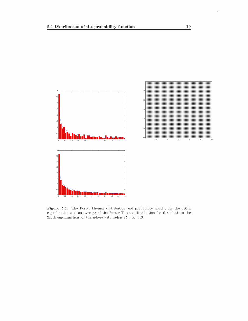
The pictures (figure 5.1, 5.2, 5.3, 5.4, 5.5) show the probability density, |ψ|2, forthe 200th eigenfunction and the Porter-Thomas distribution for the 200th eigen-function. There is a statistical fluctuation in the Porter-Thomas distribution andto get rid this the average of the Porter-Thomas distribution for the 190th to the210th eigenfunction is made. Pictures from different systems: spheres with radiiR = 1000 ×B, R = 50 ×B, R = 3 ×B, R = 2 ×B and R = 1.5 ×B

0 0.2 0.4 0.6 0.8 1 1.2 1.4 1.6 1.8 20

0.5

1

1.5

2

2.5

3

3.5

4

10 20 30 40 50 60

10

20

30

40

50

60

0 0.2 0.4 0.6 0.8 1 1.2 1.4 1.6 1.8 20

0.5

1

1.5

2

2.5

3

3.5

4

Figure 5.1. The Porter-Thomas distribution and probability density for the 200theigenfunction and an average of the Porter-Thomas distribution for the 190th to the210th eigenfunction for the sphere with radius R = 1000 × B.

5.1 Distribution of the probability function 19

0 0.2 0.4 0.6 0.8 1 1.2 1.4 1.6 1.8 20

0.5

1

1.5

2

2.5

3

3.5

4

10 20 30 40 50 60

10

20

30

40

50

60

0 0.2 0.4 0.6 0.8 1 1.2 1.4 1.6 1.8 20

0.5

1

1.5

2

2.5

3

3.5

4



0 0.2 0.4 0.6 0.8 1 1.2 1.4 1.6 1.8 20

0.5

1

1.5

2

2.5

3

3.5

4

10 20 30 40 50 60

10

20

30

40

50

60

0 0.2 0.4 0.6 0.8 1 1.2 1.4 1.6 1.8 20

0.5

1

1.5

2

2.5

3

3.5

4


5.1 Distribution of the probability function 21

0 0.2 0.4 0.6 0.8 1 1.2 1.4 1.6 1.8 20

0.5

1

1.5

2

2.5

3

3.5

4

10 20 30 40 50 60

10

20

30

40

50

60

0 0.2 0.4 0.6 0.8 1 1.2 1.4 1.6 1.8 20

0.5

1

1.5

2

2.5

3

3.5

4



0 0.2 0.4 0.6 0.8 1 1.2 1.4 1.6 1.8 20

0.5

1

1.5

2

2.5

3

3.5

4

10 20 30 40 50 60

10

20

30

40

50

60

0 0.2 0.4 0.6 0.8 1 1.2 1.4 1.6 1.8 20

0.5

1

1.5

2

2.5

3

3.5

4

Figure 5.5. The Porter-Thomas distribution and probability density for the 200theigenfunction and an average of the Porter-Thomas distribution for the 190th to the210th eigenfunction for the sphere with radius R = 1.5 × B.

5.2 The Porter-Thomas distribution for different eigenfunctions 23

5.2 The Porter-Thomas distribution for different

eigenfunctions

Chaotic behaviour is shown better for eigenfunctions with higher energy [3].

5.2.1 Results

We can see a difference in the Porter-Thomas distribution for different eigenfunc-tions. The higher number eigenfunctions follow the Porter-Thomas distributionbetter than the lower ones. The lower energy eigenfunctions show a more smeardout distribution of the probability density.

5.2.2 Pictures

The pictures (figure 5.6, 5.7, 5.8) show the Porter-Thomas distribution for thesame system, but for different eigenfunctions. The 50th, 100th, 150th and the200th eigenfunction for the systems with the radii R = 1000×B, R = 50×B andR = 2 ×B.

0 0.2 0.4 0.6 0.8 1 1.2 1.4 1.6 1.8 20

0.5

1

1.5

2

2.5

3

3.5

4

0 0.2 0.4 0.6 0.8 1 1.2 1.4 1.6 1.8 20

0.5

1

1.5

2

2.5

3

3.5

4

0 0.2 0.4 0.6 0.8 1 1.2 1.4 1.6 1.8 20

0.5

1

1.5

2

2.5

3

3.5

4

0 0.2 0.4 0.6 0.8 1 1.2 1.4 1.6 1.8 20

0.5

1

1.5

2

2.5

3

3.5

4

Figure 5.6. The Porter-Thomas distribution of the 50th, 100th, 150th and 200th eigen-function for the radius R = 1000 × B.


0 0.2 0.4 0.6 0.8 1 1.2 1.4 1.6 1.8 20

0.5

1

1.5

2

2.5

3

3.5

4

0 0.2 0.4 0.6 0.8 1 1.2 1.4 1.6 1.8 20

0.5

1

1.5

2

2.5

3

3.5

4

0 0.2 0.4 0.6 0.8 1 1.2 1.4 1.6 1.8 20

0.5

1

1.5

2

2.5

3

3.5

4

0 0.2 0.4 0.6 0.8 1 1.2 1.4 1.6 1.8 20

0.5

1

1.5

2

2.5

3

3.5

4


5.2 The Porter-Thomas distribution for different eigenfunctions 25

0 0.2 0.4 0.6 0.8 1 1.2 1.4 1.6 1.8 20

0.5

1

1.5

2

2.5

3

3.5

4

0 0.2 0.4 0.6 0.8 1 1.2 1.4 1.6 1.8 20

0.5

1

1.5

2

2.5

3

3.5

4

0 0.2 0.4 0.6 0.8 1 1.2 1.4 1.6 1.8 20

0.5

1

1.5

2

2.5

3

3.5

4

0 0.2 0.4 0.6 0.8 1 1.2 1.4 1.6 1.8 20

0.5

1

1.5

2

2.5

3

3.5

4



5.3 Amplitude distribution of the eigenfunction

Chaotic behaviour can be shown by the distribution of amplitudes of ψ (see section2.3).The amplitudes of the eigenfunction is spread equally on both sides of zero. Am-plitudes with the value zero have the highest rate. For a non-chaotic system therate goes down as the absolute value of the amplitude goes up until it reaches amaximum value, then the rate goes down to zero. For a chaotic system there isa small possibility for extremely high values of amplitudes. The distribution of

the amplitudes follow the Gaussian clock function, P (ψ) = 1σ√

2πexp(−ψ

2

2σ2 ) [3]. In

this thesis the the Gaussian curve has been approximated the fit the amplitudedistribution.

5.3.1 Results

The pictures show that the amplitude distribution follows the Gaussian curvebetter and better with decreased radius and for increased energy.

5.3.2 Pictures

The numerical results show (figure 5.9, 5.10, 5.11) the amplitude distribution and aGaussian function to match the distribution for the radii R = 1000×B, R = 40×Band R = 2×B and the eigenfunction, for which the amplitude distribution is made.Chaotic behavior is shown better for eigenfunctions with higher energy. There-fore, a comparison of the amplitude distribution for different eigenfunctions for thesame system is shown in figure 5.12.The picture shows the amplitude distributionsfor the 50th, 100th, 150th and the 200th eigenfunction in the system with theradius R = 2 ×B.

5.3 Amplitude distribution of the eigenfunction 27

−4 −3 −2 −1 0 1 2 3 40

0.05

0.1

0.15

0.2

0

10

20

30

40

50

60

0

10

20

30

40

50

60−0.04

−0.03

−0.02

−0.01

0

0.01

0.02

0.03

0.04

Figure 5.9. The distribution of the amplitudes and 200th eigenfunction for the radiusR = 1000 × B.

−4 −3 −2 −1 0 1 2 3 40

0.05

0.1

0.15

0.2

Steps=25R=40 Nr 200 Grid 60*60

010

2030

4050

60

0

10

20

30

40

50

60−0.04

−0.03

−0.02

−0.01

0

0.01

0.02

0.03

0.04

Figure 5.10. The distribution of the amplitudes and the 200th eigenfunction for theradius R = 40 × B.


−8 −6 −4 −2 0 2 4 6 80

0.05

0.1

0.15

0.2

0.25

0.3

0.35

0.4

0

10

20

30

40

50

60

0

10

20

30

40

50

60−0.06

−0.04

−0.02

0

0.02

0.04

0.06

0.08

Figure 5.11. The distribution of the amplitudes and the 200th eigenfunction for theradius R = 2 × B.

5.3 Amplitude distribution of the eigenfunction 29

−6 −4 −2 0 2 4 60

0.1

0.2

0.3

0.4

0.5

−6 −4 −2 0 2 4 60

0.05

0.1

0.15

0.2

0.25

0.3

0.35

0.4

0.45

0.5

−6 −4 −2 0 2 4 60

0.05

0.1

0.15

0.2

0.25

0.3

0.35

0.4

−8 −6 −4 −2 0 2 4 6 80

0.05

0.1

0.15

0.2

0.25

0.3

0.35

0.4

Figure 5.12. The amplitude distribution of the 50th, 100th, 150th and 200th eigenfunc-tion for the radius R = 2 × B.

Chapter 6

Show the curvature

Finally a picture below shows that the system really is a curved surface. It isshown best for the eigenfunction for a sphere with small radius. Here is the firsteigenfunction for a system of the box on a sphere with radius R = 1.5×B in figure6.1. It shows that the box really is square.

−2−1

01

2

−1−0.8−0.6−0.4−0.200.20.40.60.810.4

0.6

0.8

1

1.2

1.4

1.6

Figure 6.1. The first eigenfunction in [x,y,z]-space

31

32 Show the curvature

Chapter 7

Limits and tips for the

reader

7.1 Resolution of the FDM

The accuracy of the simulation depends on the resolution of the FDM in Eq.(3.10) (the size of a and b compared to B). With a higher number of grid points(higher values of rows and columns in the Schrodinger matrix) the space betweenthem (a and b) decreases (compared within the same system). A higher numberof grid points increases the scale of calculations and the time for each simulationincreases.

7.2 Better resolution of the box

More grid points make a better definition of the square on the surface, becausethe grid points get closer to the edge of the square. The total area of the box iscalculated as the sum of the area element of the grid points restriced by potetialenergy part of the Hamiltonian matrix (see section 3.3). The total area of the boxis used in some of the calculations, for example, the Porter-Thomas distribution.The area is supposed to be 2Bx × 2Bz, but the numerical one is less than that.

7.3 The smallest sphere posible

Another limit is the smallest radius possible. If the dimensions of the box are(2 × Bz) × (2 × Bx) the theoretical limit would be if the box covered the wholehalf sphere, 2R = 2

√2B ↔ R =

√2B ≈ 1.41 × B. But because of the singularity

for the angles θ = 0 and θ = 2 × π in Eq. (3.10) the program only works downto R = 1.5 × Bz. But with a higher number of grid points it is possible to comecloser to the edges, θ = 0 and θ = 2 × π.

33

34 Limits and tips for the reader

Chapter 8

Discussion and conclusion

First the results from the different chapters are shown, then there is a generalconclusion.

8.1 The eigenfunctions ψ and the probability den-

sity |ψ|2

It looks like there are less and higher amplitude peaks for the 200th eigenfuntionfor smaller radii. The probability density functions show less order for smallerradii.

8.2 Porter-Thomas

Because of the poor resolution of the grid (discussed in section 7.1), the θ−φ−gridlooks almost square for systems with larger radii than 5 × B, as it is not forthe systems with smaller radii (see figure 3.3). Therefore the pictures showingthe Porter-Thomas distribution look almost the same for the systems with largerradius than 5 × B. To get the same scale on the pictures showing the Porter-Thomas distribution the pictures only show the distribution for the probabilitydensity, ρ R 2. Therefore more chaotic systems, systems with larger maximum ofρ do not show their actual distribution. If they did, they would probably showa better correspondence to the curve all the way up to the maximum of ρ, forwhich the distribution is zero. The more regular systems only follow the curve upto their maximum of ρ, for which the distribution is larger than zero. Comparewith the distribution of the amplitudes (see figures in section 5.3.2). The totalarea of the box is not exactly as big as it should be (discussed in section 7.2) andit is different for the different systems. Therefore, the calculations of the Porter-Thomas distribution do not only depend on how regular the systems are, but alsoon the error in the summation of the total area. The statistics is made on all gridpoints. The grid points, which lay outside the box are multiplied with zero (see

35

36 Discussion and conclusion

figure 3.3). So the distribution of the value around zero is too large and thereforethe distribution of the other values is too small.

8.3 Amplitude distribution and Gaussian clock

curve

The large pile around zero is an effect of how the systems were modelled. In thegrid points, where the potential matrix elements are not zero (see figure 3.3), thefunction is zero. These elements do not belong to the system and therefore therate distribution of the amplitudes equal zero is larger than it should be. It showsthat the distribution follows the Gaussian clock curve better and better with adecreased radius and for functions with larger energy.

8.4 Conclusion

All the pictures indicate that the distributions follow the theoretical curves betterfor a smaller radius. The distributions do not follow the curves perfectly. But if itwas possible to decrease the radius of the sphere even more, it could be an almostperfect match. But it is not possible to decrease the radius of the sphere more, sothe hypothesis is not true.

Bibliography

[1] P. A. Tipler, R. A. Llewellyn, Modern Physics Fourth edition (W. H. Freemanand Company, New York, U.S.A., 2003)

[2] K-F. Berggren, Kvantkaos, KOSMOS 2001: 43-64, Svenska Fysikersamfundet(2001)

[3] H. J. Stockmann, Quantum Chaos: An Introduction (Cambridge UniversityPress, Cambridge, U.K.,1999), and references cited therein.

[4] C. C. Chen, C. C. Liu, K. W. Su, T.H. Lu, Y.F. Chen, and K. F. Huang,Phys Rev, E vol. 75, p. 046202 (2007)

[5] Arieh Iserles, A First Course in the Numerical Analysis of the DifferentialEquations (University Press, Cambridge, U.K., 2003)

[6] C. Nordling, J. Osterman, Physics Handbook for Science and EngineeringSixth edition (Studentlitteratur, Lund, Sweden, 1999)

37

38 Bibliography

quantum chaos on a curved surface - diva portal126936/fulltext02.pdf · quantum chaos on a curved...

Documents