Physica D 33 (1988) 77-88 North-Holland, Amsterdam

QUANTUM CHAOS: LOCALIZATION VS. ERGODICITY

B.V. CHIRIKOV, F.M. IZRAILEV and D.L. SHEPELYANSKY Institute of Nuclear Physics, 630090, Nooosibirsk, USSR

Received 14 January 1988

Results of theoretical and numerical studies of the quantum chaos are presented, and our current understanding of this phenomenon is discussed. The main attention is focused on the localization and ergodicity in classically fully chaotic quantum models, and on the related statistical properties of energy spectra as well as of eigenfunctions.

1. Introduction

The quantum chaos, a mysterious counterpart of the classical dynamical chaos is one of the most intriguing problems in physics currently under extensive studies by many researchers throughout the world. Professor Joseph Ford first addressed this difficult and exciting issue at the 1977 Como conference on Stochastic Behaviour in Classical and Quantum Hamiltonian Systems, organized by himself and Giulio Casati [1]. It was the first attempt to bring together various scientists who at that time worked separately in essentially the same direction. Joe Ford has greatly contributed to this field not only by studying and solving many par- titular problems but also by giving very interest- ing and original thoughts to the philosophy of dynamical chaos, both classical and quantal [2]. The present paper is a fragment in our current understanding of the phenomenon of quantum chaos which is gradually emerging, particularly from numerous discussions, and disputes, with Joe Ford.

Our starting point is the dynamical chaos in classical mechanics, or in the classical limit of quantum mechanics, as we usually say. This phe- nomenon is well understood by now (see, e.g. refs. [3, 4]). We think of dynamical chaos as random motion (in the sense of Alekseev) of a purely

dynamical system without any random parameters or any noise. According to the Alekseev-Brudno theorem (see ref. [5]) the necessary and sufficient condition for such a chaos is exponential local instability of motion on a set of initial conditions of dimension greater than one (to exclude the case of an isolated unstable periodic trajectory). Be- sides, the motion must be bounded, at least in some dynamical variables. The instability rate is characterized by the metric entropy h of Kolmogorov and Sinai (whose notation should not be confused with Planck's constant h). The ran- dom (chaotic) motion remains unpredictable after any number of preceding measurements with any finite accuracy, nor is it reproducible by any finite (cellular) automaton (in particular, by a digital computer).

The ultimate origin of dynamical chaos lies in the continuity of the phase space in classical mechanics which implies an infinite amount of information related to almost any exactly fixed dynamical trajectory. The mechanism of local in- stability "unfolds" this information in time, so that asymptotically as t ~ o¢ the specific informa- tion per unit time approaches the limiting value J(t)/Itl ~ h [5]. The time interval tp, on which a partial prediction is still possible (" temporal de- terminism"), depends on the observation accuracy e, and it is determined by the randomness parame-

0167-2789/88/$03.50 © Elsevier Science Publishers B.V. (North-Holland Physics Publishing Division)

78 B. V. Chirikov et al. / Quantum chaos

ter [61:

hit[ Itl (1.1) R = - ~ e l tp "

For I tl < tp (R _< 1) a statistical description is also possible if e is small enough while for R >> 1 it is the only possibility ("asymptotic randomness"). Notice that randomness of the motion alone does not determine its statistical properties, which may happen to be rather unusual (see, e.g., ref. [7]).

Turning now to the more profound quantum mechanics we, first, separate the problem into two unequal parts: (i) the proper quantum dynamics that is the time evolution, including stationary states, of the state vector q'(t), and (ii) the mea- surement with its unavoidable statistical effect of the irreversible g' collapse which is a sort of inevitable noise. In accordance with our dynami- cal approach, we shall restrict ourselves to the first problem only, as the other researchers in this field also do. To be more accurate, we assume that there are two measurements only: the first (com- plete) one fixes the initial state of a system while the second records the result of its evolution. Notice that unlike in classical mechanics, any in- termediate measurement would generally change the quantum motion considerably.

In what follows we will discuss only Hamilto- nian (nondissipative) systems, considering them to be the more fundamental ones. Phenomenological friction is but a crude approximation of the molecular Hamiltonian chaos which is inevitably related to some noise according to the fluctua- t ion-dissipation theorem.

Furthermore, we are most interested in con- servative systems with the energy surfaces closed in phase space. In this case the principal peculiar- ity of quantum mechanics - the phase space dis- c re teness- manifests itself in a most explicit way which implies, in turn, the discreteness of the energy (and frequency) spectrum. The latter is not only incompatible with dynamical chaos but, in classical mechanics, is characteristic of the oppo- site limiting case, the regular motion. However,

the fundamental correspondence principle re- quires some transition to chaos in the semi- classical region. How could it be possible? This question has been posed and answered in ref. [8] by means of introducing characteristic time scales of quantum evolution.

The shortest (logarithmic) scale t E, which we will term Ehrenfest's scale, is of the order

ht E - lnq, (1.2)

where h is the metric entropy (see above), and q - h -1 is some characteristic quantum p a r a m e t e r - a quantum number, for example (see also section 3 below). Apparently, this time scale was first discovered in ref. [9] (see also refs. [10, 8]). It is explained by the fast spreading of a narrow wave packet because of the local instabil- ity of chaotic motion in the classical limit. Accord- ing to Ehrenfest's theorem, a narrow packet fol- lows the classical trajectory, hence its motion, on scale tE, is as random as in the classical limit. However, upon a complete quantum measurement the quantity e in eq. (1.I) reaches its minimal value, - l / q , hence R - 1, and the whole Ehren- lest scale falls into the domain of temporal de- terminism.

Even though Ehrenfest's scale grows very slowly with q, it grows indefinitely as q ---, o¢ (h ~ 0). It is sufficient to provide transition to the classical chaos. However, it turns out that there exists a much longer (power law) scale t D of quantum dynamics which is obviously a more important one. It is given by

In (COtD) - - lnq . (1.3)

Here co is a characteristic classical frequency. On this (longer) scale, some important features of the classical chaos still persist, such as diffusion and statistical relaxation. This "diffusion scale" has been discovered in numerical experiments [1], and was explained in ref. [8]. Just this scale is going to be considered below (sections 4 and 5).

B. V. Chirikov et aL / Quantum chaos 79

As t ---> oo (t >> tD) the quantum nature of the evolution becomes decisive at any q ~ oo, and dynamical chaos manifests itself in a peculiar sta- tistics of energy levels as well as in the structure of eigenfunctions (sections 6 and 7).

momenta (cf. eq. (2.2))

3gk h i = - - l l k ~ 0 i " (2.5)

2. An example of true quantum chaos

The principal result of recent extensive studies in quantum chaos was the conclusion on its ab- sence as was first pointed out by Krylov [11] in the late forties. However, there are some special cases when the true dynamical chaos proves to be possi- ble in quantum mechanics as well.

Consider a classical dynamical system on an N-dimensional torus with angle variables 01:

4 = g i ( O k ) , i , k = 1 . . . . . N. (2.1)

Then, in the case of time-reversible dynamics, for example, the momenta also grow exponentially (2.3).

Now, consider a quantum system with Hamilto- nian operator [12]

I ~ = ½ ( g k h k + ~ k g k ) , ~k = - - ioe k. (2.6)

Schr~Sdinger's equation implies

~p 3 ~----f + -~k (ogl,) = 0, (2.7)

Here the functions & are of period 2~r in all 0 k. The chaos is possible in such a system for N > 3 (see, e.g., ref. [3]). It means that the equations of motion linearized about some trajectory O°(t)

~,={k~-~k , (2.2)

where ~i ~" Oi - - 07, are exponentially unstable, that is

~ i - ea ' t - (2.3)

Here A m is the maximal Lyapunov exponent of the linear system (2.2).

The dynamics of system (2.1) can be described, for any functions gi, by the conserved Hamilto- nian

where p = ff'~/,* is the probability density, which coincides with the continuity equation for the classical system (2.1). Hence, the quantum prob- ability would evolve exactly in the same way as the classical one, including the case of chaotic motion [12].

This simple example clearly demonstrates how extraordinary chaotic quantum dynamics has to be. Besides unbounded motion in momenta the latter are to grow exponentially fast. This is be- cause the fine-grained (exact) probability density does not become homogeneous in time, as the coarse-grained density does; on the contrary, the former becomes more and more "scarred" by the mechanism of local instability of trajectories. This implies a fast growth of wave numbers, and, in quantum mechanics, of momenta.

H = nkgk(Oi), (2.4)

which implies the equations for the conjugate

3. The quantum rotator model

For studying the dynamics of classically chaotic quantum systems we have chosen the model of a

80 B. V. Ch i r i kov et a l l Q u a n t u m chaos

quantum rotator specified by the Hamiltonian [1]

~2 / - I= -~- + k cos 0 . 8 r ( t ) . (3.1)

Here the momentum is ~ = - i ~ / 3 0 ; 0 is the conjugate phase; V= k cos 0 is the perturbation function; 8 r ( t ) is the delta-function of period T, and we have set h = 1. The dynamics of the corre- sponding classical system is described by the

standard map [13]

f i = p + K s i n O ' 0 = 0 + f i , (3.2)

where p = Tn, and K= kT. The classical limit here corresponds to k ---, oo, T ---, 0 while K = kT = const.

The dynamics of the quantum model (3.1) is

also specified by a unitary mapping

g , = e x p i ~ - - ~ e x p ( - i k c o s 0 ) q " (3.3)

and, unlike the classical model, essentially de- pends on both parameters k and T. In this model the perturbation is periodic in time. We mention that many particular physical problems can be reduced to such a model (see, e.g., ef. [14]).

Studying a map (especially numerically) is much simpler than a continuous model. This was pre- cisely the main reason to choose model (3.1) from

the beginning. As we shall see fight now the potential richness

of this "simple" model is still far from being exhausted (see also ref. [7]). Particularly, system (3.1) may be thought of as a model of conservative dynamics, too. Indeed, in the classical limit a two-dimensional map of type (3.2) is related to some conservative system of two degrees of free- dom (see, e.g., ref. [3]). Thus, such a map describes the local dynamics on the energy surface. To some extent, this should be true for the quantum map (3,3) as well.

Moreover, the model (3.1) can be modified to represent the global dynamics of a conservative system [16]. To this end we "close up" the

momentum axis p of the classical model (3.2) over some period P0, so that the infinite phase cylinder of map (3.2) is converted into a finite torus. The map remains smooth if Po = 2~rrn0, with m 0 an integer. Then the period in n is N = 2~rmo/T, which is also the full number of quantum states for model (3.1) on a toms. Hence the quantity T/2~r = mo/N is bound to be rational. For in- finite quantum map (3.3) on a cylinder this would imply a very peculiar dynamics, the so-called quantum resonance [1, 15]. In the theory of this quantum phenomenon [15] the quantum map (3.3) is represented by a finite-dimensional unitary ma- trix U,,, of some dimension N.

To apply this theory to the finite quantum model on a torus, we may simply pick out only the solutions '/ '(n, "r) that are periodic in n in the momentum representation, and understand them as a finite Fourier series:

NI • (0, ~') = Y'. g ' (n , ~') e i"°, (3.4)

n = -- N 1

where N = 2N 1 + 1 is odd, and ~- is the number of map iterations.

The corresponding unitary matrix is conveni- ently represented in the following symmetric form:

v , . . = (3.5)

where the diagonal matrix

Gu, = 8,,,exp ( ~ l 2 ) (3.6)

describes a free rotation over time 7"/2, while the matrix

( B , , , = ~ Y'~ exp - i k c o s l I= -- N 1

× e x p ( - i ~ l ( m - n ) ) . (3.7)

represents the effect of the perturbation (a "kick"). In the semi-classical limit, the additional condi-

B. E Chirikov et al./ Quantum chaos 81

tion N T = 2 ~ m o = c o n s t ( N ~ ) should be satisfied. "Energy" levels t0q of this model are always within the interval (0, 2¢r), and are related to the eigenvalues hq of the unitary matrix Umn by the expression X = exp (ito).

Similar models on a sphere, rather than on a torus, were also studied (see, e.g., ref. [17]).

The dynamics of the classical infinite model (3.2) is completely determined by a single parame- ter K. Depending on its value there are two dif- ferent regimes of motion: (i) bounded (IAnl < v/-k/T), and (ii) unbounded. The critical K value separating them is most likely to be Kcr = 0.9716.. . - -1 [18]. Notice that in both regimes regular and chaotic components of motion coexist, the measure of the former vanishing as K grows [13].

At K > Kcr the motion in the connected chaotic component may be described as a diffusion in n with the rate

<(An) 2) Do(K ) D = ~" T2 , (3.8)

where Do(K ) is the diffusion rate in p for the map (3.2); ~" the number of iterations.

In the semiclassical region, the classical diffu- sion persists within the diffusion time scale which is of the order z t~- D - k 2 [8]. For ~" << "i'D the quantum dependence Dq(K) mimics all the details of the classical diffusion [19] in accordance with the correspondence principle.

The quantum diffusion stops for z >> ZD, and turns into a stationary oscillation which was ob- served up to ~" = 5 × 104 [20]. This would imply a discrete quasienergy spectrum for model (3.1) [8]. Hence, the "quantum chaos" is not true chaos as in the classical limit. Notice that deviations from the latter already begin on a much shorter scale (1.2) where q = k. Particularly, the local instability of quantum motion disappears at ~" > zE [21, 22] while residual correlations persist [21, 23] (see also ref. [4]).

A striking illustration of dynamical stability in quantum chaos is afforded by a numerical experi-

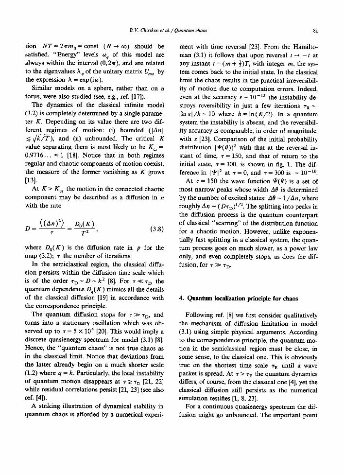
ment with time reversal [23]. From the Hamilto- nian (3.1) it follows that upon reversal t--* - t at any instant t = (m + ½)T, with integer m, the sys- tem comes back to the initial state. In the classical limit the chaos results in the practical irreversibil- ity of motion due to computation errors. Indeed, even at the accuracy e - 10 -12 the instability de- stroys reversibility in just a few iterations ~'R- I l n e l / h - 10 where h - - l n ( K / 2 ) . In a quantum system the instability is absent, and the reversibil- ity accuracy is comparable, in order of magnitude, with e [23]. Comparison of the initial probability distribution I xr,(O)l 2 with that at the reversal in- stant of time, ~-= 150, and that of return to the initial state, ~" = 300, is shown in fig. 1. The dif- ference in I q[ 2 at • = 0, and ~- = 300 is - 10-10.

At "r = 150 the wave function xo(8) is a set of most narrow peaks whose width A0 is determined by the number of excited states: A0 ~ l /An , where roughly An - (D,rD) 1/2. The splitting into peaks in the diffusion process is the quantum counterpart of classical "scarring" of the distribution function for a chaotic motion. However, unlike exponen- tiaUy fast splitting in a classical system, the quan- tum process goes on much slower, as a power law only, and even completely stops, as does the dif- fusion, for z >> rD-

4. Quantum localization principle for chaos

Following ref. [8] we first consider qualitatively the mechanism of diffusion limitation in model (3.1) using simple physical arguments. According to the correspondence principle, the quantum mo- tion in the semiclassical region must be close, in some sense, to the classical one. This is obviously true on the shortest time scale ~'E until a wave packet is spread. At ~- > '/'E the quantum dynamics differs, of course, from the classical one [4], yet the classical diffusion still persists as the numerical simulation testifies [1, 8, 23].

For a continuous quasienergy spectrum the dif- fusion might go unbounded. The important point

82 B.V. Chirikov et al. / Quantum chaos

is that in case of a discrete spectrum, with mean

level densi ty Po, the diffusion can still go on during

a finite t ime interval

- ~D - Po- (4.1)

It is directly inferred f rom the uncertainty princi-

ple that for ~-<< P0 the system does not resolve ("does not feel") the spectrum discreteness pro-

vided the transitions between unper turbed states

are efficient enough, that is, the per turbat ion ex-

ceeds Shuryak's quan tum border of stability [29].

In model (3.1) the latter is at k - 1 [1, 8]. Estimate

(4.1) gives the diffusion time scale ~'D for model

(3.1). It is impor tant that the density Po in eq. (4.1)

is determined by those eigenfunctions only which are actually present in a given quan tum state, their

effective number being always finite.

~0

a

M

-I.0 -0,o 1.0

~.8 IY IO)I~

oo 0

• i . . . . . . . . . I ' . . . . . . . . I . . . . . . . " ' ' i : : : : : : I : : ~ : : : ~ : I : : : : : : : : : I ~ : : = -~.14 -2.14 -LI4 -OJ~ 0.86 1.86 2.g6

Fig. 1. Probability distribution in model (3.1) at different instances of time (k = 20; K = 5): (a) ~" = 0, initial Gaussian distribution (lower curve); ~" = 300, final distribution (upper curve, shifted upwards); (b) ~" = 150, time reversal.

B. V. Chirikov et al. / Quantum chaos 83

Consider, first, the evolution of a single unper- turbed state. The number of neighbouring unper- turbed states excited due to diffusion during time ~'D would be An - Dv/-D-~n. It implies that the eigen- functions are superpositions of many ( - A n ) un- perturbed states, and vice versa, any unperturbed state is represented by the same number of eigen- functions. Assuming that quasienergies are homo- geneously distributed within the interval (0,2~r)

we obtain Po - A n - ~'o, a n d

~'D -- D - A n -- l, (4.2)

where l is the effective number of unperturbed states finally excited after the diffusion is over. In other words, l is the localization length of eigen- functions in n. Remarkably, estimate (4.2) relates essentially quantum characteristics, the diffusion scale ro and the localization length l, to the diffusion rate D in the classical limit.

The estimate (4.2) for ~'D apparently does not depend on the initial state apart from very un- likely states close to the eigenfunctions. As to the localization length l for the final state of a sta- tionary distribution, eq. (4.2) holds only if the size of initial state l 0 < l. In the opposite case (10 >_ l) the size does not change at all.

5. Localization of quasienergy eigenfunctions, and of the stationary distribution

In ref. [24] a similarity was pointed out between the above-mentioned localization in momentum space (in n) and the well-known Anderson locali- zation in a one-dimensional random potential (for the latter see, e.g., ref. [25]). The most important distinction between the two phenomena is that our model (3.1) has no random parameters. Also, the mechanism of localization in our model is, gener- ally, completely different in various domains of the parameters. If K >_ 1 and k >_ 1 the localiza- tion is due to the hold-up of classical diffusion because of quantum interference effects. On the other hand, for K < 1 and k >_ 1 it is related to the

quantum tunnelling in a classically inaccessible region.

Borrowing an idea from solid state physics [25, 26], one can calculate the quantum localiza- tion length via Lyapunov exponents in an aux- iliary classical Hamiltonian system [27]. An im- portant advantage of this approach is in that one does not need to calculate the eigenfunctions, thus simplifying much of the numerical procedure. In the problem under consideration this method was also used in ref. [28].

For model (3.1) the equation for an eigenfunc- tion % with quasienergy to can be written as [27]

(k) (o ~on+~J~ -~ sin 2 4 2 = 0 ' (5.1)

where Jr is the Bessel function. Because of sharp drop of Jr at Jr I > N - k / 2 one can leave a finite number 2N + 1 - k of terms in the sum. Then, the recursion, eq. (5.1), determines a 2N-dimensional dynamic system which turns out to be the Ham- iltonian [27]. Hence, it has N positive (-/i +) and N negative (Yi-) Lyapunov exponents, and for each pair 7i++ V /= 0. Asymptotically, the localization length 1 is determined by the minimal Lyapunov exponent Y1 = 1 /1 , and the eigenfunctions behave like c p n ~ e x p ( - I n l / l ) as Inl---' oo. Hence, the quasienergy spectrum is purely discrete.

According to the theoretical estimate (4.2) the localization length is given by

l = a D = D ° ( K ) 2T 2 (5.2)

The numerical factor a = 1 has been obtained in ref. [27] by comparison with the exactly solvable Lloyd model. For this model the perturbation is V(O) = 2 arc tg(E - 2k cos 0), and, in the quasilin- ear approximation, the diffusion rate is

1 fW ave2 D = = Yo ao I dO. (5.3)

84 B. V. Chirikov et al./ Quantum chaos

Lyapunov exponents were computed using the standard techniques (see, e.g., ref. [3]) in the parameter range: 5 < k < 75; 1.5 < K < 29; T < 1 (T /4~r irrational), and D O varying by four orders of magnitude [27]. The mean value ( a ) = 0.57 + 0.02 (here and below statistical errors only are indicated). A slightly enhanced a value might be observed because the ratio k / l - 0.1 was not small

enough. Another way to check eq. (5.2) is by computa-

tion of the localization length for stationary distri- bution. Let the system be initially in state n = 0, for example. The stationary distribution for ~- >> '/'D is obtained by time averaging of probabilities I xO(n, I")12:

]:(n) ~ I'/'(n, , )1 z= E I%,(0)%,(n) 12, tYt

(5.4)

where %,(n) are the eigenfunctions. Notice that f ( n ) is the counterpart of the density-density correlation in the solid state problem [25]. Ex- ponentiaUy localized eigenfunctions may be repre- sented as

I%~(n) [ - exp ( ~ + [n-ml ~nm), (5.5)

fluctuations,

= Z),l nl,

we have, according to refs. [19, 27],

1 1 D~ l~ - t 2 ' lD~ <_ l ,

1 1 lD~ > 1,

l~ 212D~ '

(5.8)

Again, a similar phenomenon is known in solid state physics [25].

An example of the stationary distribution is shown in fig. 2. The law (5.7) is verified approxi- mately within a long range (0 < x = 2 D n I l ls <_ 25) over about 10 orders of magnitude in fN varia- tions. A large-scale structure of f N ( x ) is ap- parently related to fluctuations of ~ , , .

Numerical simulation [19] in the parameter range 5 < k < 120; 9 < l s < 180; T < 1 (D o varia- tion comprises four orders of magnitude) results

in (as) = 1.04 +_ 0.03 where a s = l s /D = lsTZ/Do (4.2), and l s was numerically determined using eq. (5.7) (see fig. 2). Thus, l s = 2l, and the diffusion rate in ~,,~ is

1 2 D~ = 7 --" D " (5.9)

where ~,,, describe fluctuations about average ex- ponential dependence, and ( ~ , , , ) = 0. Assuming that on the average

Direct computation of D~ from the fluctuations of Lyapunov exponents gives (lD~) -- 1.14 [27].

1 ( l % , ( n ) 1 2 ) = ~ e x p ( - 2 [ n - m [ ) , (5.6)

we obtain from eq. (5.4)

f ( n ) = 1 + 21nl / t s ( 21hi 1 2l s e x p - ls ]. (5.7)

It may seem strange that the distribution localiza- tion length I s is generally different from l for eigenfunctions. This is due to large fluctuations in ~.m- In the case of diffusively growing Gaussian

0

× B Io 2~ ~0

Fig. 2. Stationary distribution for k = 10; T = 0.5; K = 5. Straight line: f-N = e-X; fN = 21~](n)/(1 + x); x = 2n/ls.

B.V. Chirikov et al./ Quantum chaos 85

Above we considered the asymptotic behaviour of eigenfunctions and of the stationary distribu- tion at n >> l. Those at n - 1 are also of impor- tance as they determine, for example, the mean energy of stationary oscillations, E s = {n2) /2 . If eq. (5.7) holds, then (n 2) = l 2, and E s = D2/2. This is also in a good agreement with our numeri- cal data: ( 2 E s / D 2) = 0.92 _+ 0.04.

6. Energy level statistics

Asymptotically as t ~ oo, the time evolution of any bounded quantum system (at least, a con- servative one) is almost periodic because of its discrete energy (and frequency) spectrum irrespec- tive of the motion in classical limit. This is just the opposite to the classical chaos (hence, the term "quantum pseudochaos" [30]). Yet, "remnants" of classical chaos still persist in peculiar statistical properties of the quantum spectrum, which will be discussed in this section, and of chaotic eigenfunc- tions to be considered in the next section 7.

These statistical properties have been studied since long ago, that led to the development of the random matrix theory, a statistical theory closest to the quantum dynamics (see, e.g., refs. [31, 32]). Until recently, however, this theory had been un- derstood as some general description of a typical "complex" quantum system with many degrees of freedom. A striking resemblance to the traditional philosophy in statistical mechanics! Apparently, the relation of the statistics of quantum spectra to the dynamical chaos in classical limit was first considered in refs. [33, 34]. Much later numerical experiments on simple quantum models of only two degrees of freedom demonstrated surprisingly good agreement with random matrix theory, in- deed [35]. This important result for the energy level statistics of a conservative system has been extended in ref. [36] to the quasienergies of the time-dependent model (3.1).

Here we consider the finite model (3.5) of a conservative quantum system as explained in sec- tion 3 above. Random matrix theory, particularly,

predicts that the distribution of nearest energy level spacings has the Wigner-Dyson form [31, 32]

p ( s ) = As ~ e - Ss2, (6.1)

where A, B are normalizing constants; s the spac- ing with ( s ) = 1, and the parameter/3 = 1, 2 or 4 depends on the system's symmetry (for a new recent discussion of this dependence see refs. [36, 37]). For our finite model, /3 = 1.

In fig. 3, two characteristic examples of numeri- cal data for model (3.5)-(3.7) are shown. Because of the spatial parity conservation the eigenfunc- tions are either even or odd: xo,+(n)= _+ ~ o , ( - n ) where o~ is an "energy" eigenvalue. Both sets of eigenvalues were processed separately, and the

, S

: : : : : : : : : : : : : : : : : : : : : : : : : : : : : : : : : : : : : : : : : : : : : : : : : : :

0 ~ Z 3 tt

5 0

P~

: : : : : l ~ j ~ : : ~ : ~ : : ~ ; ~ : : : I . . . . . . . . . . . i . . . . . . . . . . . i . . . . . . . . . . . . i . . . . . . . . . . . , r

0 ~ 2 3 q

Fig. 3. Nearest energy level spacing distribution in model (3.5)-(3.7) for T= 16~/(2N~ + 1); N t = 25: (a) k --- 20; K~- 20; 1=130; A=5; (b) k=5; K--5; /~6; A ~-0.25. Curves are Wigner-Dyson distribution (6.1), fl = 1.

86 B. V. Chirikoo et al. / Quantum chaos

results were summed up. To further improve the statistics, 20 values of the parameter k were used with Ak = 0.2, the total number of energy levels amounting to 20 × 51 = 1020. The reduced spac- ing is s = N 1 Aw/2~r, where A~0 is the difference of nearest energy values, and N 1 = (N - 1) /2 = 25 the number of eigenfunctions with a given symme- try. The calculation accuracy in ~ = exp(i~0) was checked by the deviations I lXl - 11< 10 -5.

For both cases in fig. 3, the classical motion is known to be fully chaotic [13] as K = kT>> 1.

Yet, the two distributions p ( s ) reveal a striking difference. Our explanation is in that a new im- portant parameter comes here into play, namely, the ratio A = I / N 1 of the localization length (sec- tion 5) to the dimensionality of eigenfunctions in Hilbert space that is the maximal number N x of (independent) unperturbed states coupled in an eigenfunction.

In one case (fig. 3(a)) A---5 >> 1, that is, the eigenfunctions are ergodic in the full unperturbed basis (see section 7 below). As a result there is a good agreement with random matrix theory (6.1), well confirmed by the X2-criterion: X2(24)--28.6 which corresponds to a confidence level of 23 percent.

In the other case (fig. 3(b)) A = 0.25 < 1, which leads to an undisputable deviation p ( s ) from eq. (6.1). Thus, random matrix theory is applicable to classically chaotic systems under the condition A >> 1 only, and we call eq. (6.1) the "limiting statistics". The new result for A < 1 we term "in- termediate statistics" because there are good rea- sons to believe [36] that in the limit A ~ 0 the distribution p (s) ~ exp ( - s) would approach the Poisson statistics of a completely integrable sys- tem in spite of chaos in the classical limit.

An important question arises: could the inter- mediate statistics be described by a one-parameter (A) family of distributions? A similar possibility was discussed by several authors and recently rejected in ref. [38] for a different kind of inter- mediate statistics due to the presence of regular motion in classical limit. In our case, however, we believe that it is true, indeed, and there exists a

universal distribution pu ( s ,A ) connecting both limits, Poisson's and Wigner-Dyson's. Moreover, we conjecture that the localization parameter A must be related somehow to the inverse "tempera- ture" 13 (6.1) in Dyson's thermodynamical model of level repulsion [39]. This hypothesis is currently under study.

7. Chaotic structure of eigenfunctions

Even though random matrix theory considers statistical properties of both energy levels as well as eigenfunctions, until recently the former were studied almost exclusively. One reason was that the data on eigenfunctions are not directly available in laboratory experiments. However, this restriction does not take place in numerical simu- lation. The second, more profound, difficulty is that the eigenfunction structures, unlike the eigen- values, are noninvariant under rotation of the basis. Particularly, there always exists a special bas is - the eigenfunctions themselves- with trivial structure. In a sense, such bases are a priori very unlikely. In any event, it does not preclude the formulation and proof of a very important theo- rem [40] which states that in a classically ergodic system almost all eigenfunctions sufficiently far in the semiclassical region are also ergodic. In what follows we are going to make use of the unper- turbed basis.

In the spirit of random matrix theory we define ergodicity by the condition ( [~m(n) l 2> = 1 / N 1,

where q , , (n) is probability amplitude for the mth eigenfunction in the n th unperturbed state, and the normalization zULl[kOm(n ) ]2= 1 is assumed. The averaging above is over either the same eigen- function (in n), or different eigenfunctions (in m), or various matrices U,,, with different values of parameters, or any combination of the former.

The obvious condition for ergodicity is A = l / N 1 >> 1. In the semiclassical region l - k 2 ~ o o ,

and N a - m o / T - m o k / K ~ ~ so that A K k / m o ~ ~ , which leads to ergodicity in accor- dance with Shnirelman's theorem [40].

B. V. Chirikov et aL / Quantum chaos 87

A more interesting and difficult question con- cerns the fluctuations of g',,(n). Gaussian fluctua- tions were conjectured in several papers (see, e.g., refs. [41]). Here we present our numerical results for model (3.5)-(3.7).

Because the matrix U,~, is unitary and symmet- ric, the real and imaginary parts of the eigenfunc- tions coincide. Hence, it is sufficient to study the eigenfunctions of the real part Re(Urn,). An exam- ple of a distribution of the values xI,- xt,,,(n) of different odd eigenfunctions m = 1 . . . . . N 1 at dif- ferent n = 1 . . . . . N 1 for 20 different matrices U,, n is presented in fig. 4. Curve I shows the Gaussian distribution

w(,/,) = f~2--~ e-*'"J2, (7.1)

assuming ergodicity ( ~ 2 ) = l /N1 ' and (~/') = 0. At first glance the agreement is fairly good. Yet,

X2(38) = 98, and the confidence level < 10-6(!). Hence, the fluctuations are close to Gaussian ones but certainly not exactly Gaussian.

Our explanation of this surprising disagreement relies upon the finite dimensionality, N1, of the eigenfunctions. As a result, if' fluctuations are strictly bounded by the condition x~t2 _<< 1, and an exact Gaussian distribution is impossible. Instead, we assume, following random matrix theory, the eigenfunctions to be invariant under any rotation

tM

7M

lIN

IN

|

,~(v)

-3 -2 " t 0 t 2 3

Fig. 4. Fluctuat ions of chaotic eigenfunctions for the parame- ters in fig. 3(a). Curve I is Gaussian distribution (7.1); curve II the distribution (7.2).

of the basis. Then (see, e.g., ref. [32])

wNl(g') = v ~ F ~ ) ( 1 - (7.2)

where F is the gamma-function. This distribution is also shown in fig. 4 (curve II). The difference from a Gaussian distribution appears to be negli- gible. Yet, the X2-criterion (X2(38) = 56, 3 percent confidence level) clearly indicates a much better agreement of numerical data with eq. (7.2) which approaches the Gaussian distribution (7.1) in the limit N 1 ---, o0 only. This is again in agreement with random matrix theory provided the quantum system is ergodic (A >> 1), and fully chaotic in the classical limit.

An additional check of eq. (7.2) is by calcula- tion of the moments m k of distribution (7.2) normalized to unity for Gaussian distribution. Comparison of analytical and numerical results,

m(2 a) = 1,

m(2 n) = 0.996 + 0.012,

1 m~4") = 2 = 0.926,

m(4 ") = 0.888 _ 0.030,

1 = 0.798,

m (n) = 0.703 + 0.068,

also clearly shows deviations from a Gaussian distribution in agreement with random matrix the- ory. We emphasize again that unlike the later, our model has no random parameters.

During many years the present authors have greatly benefitted from permanent (though chaotic!) collaboration, discussions, and disputes with Professor Joseph Ford. May it last forever!

88 B. V. Chirikov et aL / Quantum chaos

References

[1] J. Ford et al., Lecture Notes in Physics 93 (1979) 334. [2] J. Ford, What is chaos, that we should be mindful of it?

in: Chaotic Dynamics and Fractals, M.F. Barnsley and S.G. Demco, eds. (Academic Press, New York, 1985). J. Ford, Chaos: solving the unsolvable, predicting the unpre- dictable, in: The New Physics, S. Capelin and P. Davies, eds. (Cambridge Univ. Press, Cambridge, 1986). J. Ford, Quantum chaos: Is there any? in: Directions in Chaos, Hao Bai-Lin, ed. (World Scientific, Singapore, 1987).

[3] A.J. Lichtenberg and M.A. Lieberman, Regular and Sto- chastic Motion (Springer, Berlin, 1983).

[4] G.M. Zaslavsky, Chaos in Dynamic Systems (Harwood, New York, 1985).

[5] V.M.Alekseev and M.V. Yakobson, Phys. Rep. 75 (1981) 287.

[6] B.V. Chirikov, Intrinsic stochasticity, Proc. Intern. Conf. on Plasma Physics, Lausanne (1984), vol. 2, p. 761.

[7] B.V. Chirikov and D.L. Shepelyansky, Physica D 13 (1984) 395.

[8] B.V. Chirikov, F.M. Izrailev and D.L. Shepelyansky, Sov. Sci. Rev. C2 (1981) 209.

[9] G.P. Berman and G.M. Zaslavsky, Physica A 91 (1978) 450.

[10] M. Berry et al., Ann. Phys. 122 (1979) 26. [11] N.S. Krylov, Works on the Foundations of Statistical

Physics (Princeton Univ. Press, Princeton, NJ, 1979). [12] A.N. Gorban and V.A. Okhonin, Universality domain for

the statistics of energy spectrum, preprint 29B, Inst. of Phys., Krasnoyarsk (1983).

[13] B.V. Chirikov, Phys. Rep. 52 (1979) 263. [14] G. Casati, B.V. Chirikov and D.L. Shepelyansky, Phys.

Rev. Lett. 53 (1984) 2525. [15] F.M. Izrailev and D.L. Shepelyansky, Teor. Mat. Fiz. 43

(1980) 417. [16] F.M. Izrailev, Phys. Lett. A 125 (1987) 250. [17] F. Haake, M. Kus and R. Scharf, Z. Phys. B65 (1986) 381;

Lecture Notes in Physics 282 (1987) 3. [18] J.M. Greene, J. Math. Phys. 201 (1979) 1183. [19] B.V. Chirikov and D.L. Shepelyansky, Radiofizika 29

(1986) 1041.

[20] G. Casati, J. Ford, I. Guarneri and F. Vivaldi, Phys. Rev. A34 (1986) 1413.

[21] D.L. Shepelyansky, Teor. Mat. Fiz. 49 (1981) 117. [22] M. Toda and K. Ikeda, Phys. Lett. A124 (1987) 165. [23] D.L. Shepelyansky, Physica D8 (1983) 208. [24] S. Fishman, D.R. Grempel and R.E. Prange, Phys. Rev.

A29 (1984) 1639. [25] I.M. Lifshits, S.A. Gredeskul and L.A. Pastur, Introduc-

tion into the Theory of Disordered Systems (Nauka, Moscow, 1982) (in Russian).

[26] J.L. Richard and J. Sarma, J. Phys. C14 (1981) L127. A. MacKinnon and B. Kramer, Phys. Rev. Lett. 47 (1981) 1546.

[27] D.L. Shepelyansky, Phys. Rev. Lett. 56 (1986) 677; Physica D 28 (1987) 103.

[28] R. Bltimel et al., Lecture Notes in Physics 263 (1986) 212. [29] E.V. Shuryak, Zh. Eksp. Teor. Fiz. 71 (1976) 2039. [30] B.V. Chirikov, Found. Phys. 16 (1986) 39. [31] C,E. Porter, ed., Statistical Theory of Spectra: Fluctua-

tions (Academic Press, New York, 1965). M.L. Mehta, Random Matrices (Academic Press, New York, 1967).

[32] T.A. Brody et al., Rev. Mod. Phys. 53 (1981) 385. [33] G.M. Zaslavsky and N.N. Filonenko, Zh. Eksp. Teor. Fiz.

65 (1973) 643. [34] I.C. Percival, J. Phys. B6 (1973) L229; Adv. Chem. Phys.

36 (1977) 1. [35] O. Bohigas et al., Phys. Rev. Lett. 80 (1984) 157; Lecture

Notes in Physics 209 (1984) 1. [36] F.M. Izrailev, Distribution of quasienergy level spacings

for classically chaotic quantum systems, preprint INP 84-63, Novosibirsk (1984) (in Russian); Phys. Rev. Lett. 56 (1986) 541.

[37] M. Robnik and M.V. Berry, J. Phys. A19 (1986) 669. [38] M. Robnik, J. Phys. A20 (1987) L495. [39] F.J. Dyson, J. Math. Phys. 3 (1962) 140, 157, 166. [40] A.I. Shnirelman, Usp. Mat. Nauk 29(6) (1974) 181. [41] M.V. Berry, J. Phys. A10 (1977) 2083. M. Shapiro and G.

Goelman, Phys. Rev. Lett. 53 (1984) 1714. E.J. Heller and R.L. Sunberg, in: Chaotic Behaviour in Quantum Sys- tems, G. Casati, ed. (Plenum, New York, 1985), p. 255. B.V. Chirikov, Phys. Lett. A108 (1985) 68.