quantum algorithms tutorial - pqcrypto this tutorial: get to know your enemy! 3/ 37 quantum bits i...

1/ 37

Quantum Algorithms

Tutorial

Ronald de Wolf

2/ 37

Post-quantum cryptography

I Quantum computers can break public-key cryptography thatis based on assuming hardness of factoring, discrete logs, anda few other problems

I Post-quantum cryptography tries to design classical cryptoschemes that cannot be broken e�ciently by quantumalgorithms

I Classical codemakers vs quantum codebreakers

I This tutorial:

Get to know your enemy!

3/ 37

Quantum bits

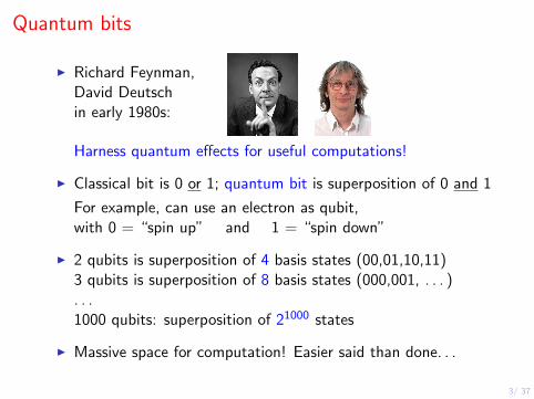
I Richard Feynman,David Deutschin early 1980s:

Harness quantum e↵ects for useful computations!

I Classical bit is 0 or 1; quantum bit is superposition of 0 and 1

For example, can use an electron as qubit,with 0 = “spin up” and 1 = “spin down”

I 2 qubits is superposition of 4 basis states (00,01,10,11)3 qubits is superposition of 8 basis states (000,001, . . . ). . .1000 qubits: superposition of 21000 states

I Massive space for computation! Easier said than done. . .

4/ 37

A bit of math: states

I 1-qubit basis states: |0i =✓

10

◆and |1i =

✓01

◆

I Qubit: superposition ↵0

|0i+ ↵1

|1i =✓↵0

↵1

◆2 C2

I

2-qubit basis state: |10i = |1i ⌦ |0i =✓

01

◆⌦✓

10

◆=

0

BB@

0010

1

CCA

I n-qubit state: | i =X

x2{0,1}n↵x |xi 2 C2

n

I Axiom: measuring state | i gives |xi with probability |↵x |2

I HenceX

x2{0,1}n|↵x |2 = 1, so | i is a vector of length 1

5/ 37

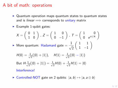
A bit of math: operations

I Quantum operation maps quantum states to quantum statesand is linear =) corresponds to unitary matrix

I Example 1-qubit gates:

X =

✓0 11 0

◆, Z =

✓1 00 �1

◆, T =

✓1 00 e⇡i/4

◆

I More quantum: Hadamard gate =1p2

✓1 11 �1

◆

H|0i = 1p2

(|0i+ |1i), H|1i = 1p2

(|0i � |1i)

But H 1p2

(|0i+ |1i) = 1p2

H|0i+ 1p2

H|1i = |0i

Interference!

I Controlled-NOT gate on 2 qubits: |a, bi 7! |a, a� bi

6/ 37

Quantum circuits

I A classical Boolean circuit consists ofAND, OR, and NOT gates on an n-bit register

I A quantum circuit consists ofunitary quantum gates on an n-qubit register(allowing H, T , and CNOT gates su�ces)

Example:

inputqubits

|0i

|0i -

-C

H -

-

-finalstate

|00i H⌦I�! 1p2

(|00i+ |10i) CNOT�! 1p2

(|00i+ |11i)

This circuit creates an EPR-pair: entanglement!

7/ 37

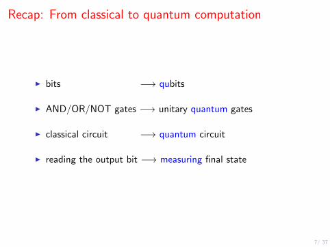
Recap: From classical to quantum computation

I bits �! qubits

I AND/OR/NOT gates �! unitary quantum gates

I classical circuit �! quantum circuit

I reading the output bit �! measuring final state

8/ 37

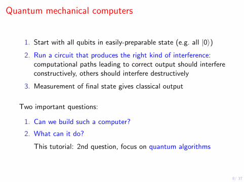
Quantum mechanical computers

1. Start with all qubits in easily-preparable state (e.g. all |0i)

2. Run a circuit that produces the right kind of interference:computational paths leading to correct output should interfereconstructively, others should interfere destructively

3. Measurement of final state gives classical output

Two important questions:

1. Can we build such a computer?

2. What can it do?

This tutorial: 2nd question, focus on quantum algorithms

9/ 37

Quantum parallelism

I Suppose classical algorithm computes f : {0, 1}n ! {0, 1}m

I Convert this to quantum circuit U : |xi|0i 7! |xi|f (x)iI We can now compute f “on all inputs simultaneously”!

U

0

@ 1p2n

X

x2{0,1}n|xi|0i

1

A =1p2n

X

x2{0,1}n|xi|f (x)i

I This contains all 2n function values!

I But observing gives only one random |xi|f (x)iAll other information will be lost

I More tricks needed for successful quantum computation

Interference!

10/ 37

Deutsch-Jozsa problem

I Given: function f : {0, 1}n ! {0, 1} (2n bits) , s.t.(1) f (x) = 0 for all x (constant),or(2) f (x) = 0 for 1

2

· 2n of the x ’s (balanced)

I Question: is f constant or balanced?

I Classically: need at least 1

2

· 2n + 1 steps (“queries” to f )

I Quantumly: O(n) gates su�ce, and only 1 query

I Query: application of unitary Of : |x , 0i 7! |x , f (x)iI More generally: Of : |x , bi 7! |x , b � f (x)i (b 2 {0, 1})I NB using |�i = H|1i, we can get queried bit as a ±-phase:

Of |xi|�i = (�1)f (x)|xi|�i

11/ 37

Deutsch-Jozsa algorithm

|0i

|0i

|1i

measure

H...

H

H

H...

H

H

Of

I Starting state: |0 . . . 0| {z }n

i|1i

I After first Hadamards:1p2n

X

x2{0,1}n|xi|�i

I Make one query:1p2n

X

x2{0,1}n(�1)f (x)|xi|�i

I Forget about the last qubit |�i

12/ 37

Deutsch-Jozsa (continued)

I After second Hadamard:

1p2n

X

x2{0,1}n(�1)f (x)

1p2n

X

y2{0,1}n(�1)x ·y |yi

I ↵0...0 =

1

2n

X

x2{0,1}n(�1)f (x) =

⇢1 if constant0 if balanced

I Measurement gives right answer with certainty

I Big quantum-classical separation: O(n) vs ⌦(2n) steps

I But the problem is e�ciently solvable by bounded-errorclassical algorithm (just query f at a few random x)

13/ 37

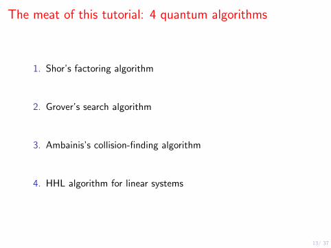
The meat of this tutorial: 4 quantum algorithms

1. Shor’s factoring algorithm

2. Grover’s search algorithm

3. Ambainis’s collision-finding algorithm

4. HHL algorithm for linear systems

14/ 37

Factoring

I Given N = p · q, compute the prime factors p and q

I Fundamental mathematical problem since Antiquity

I Fundamental computational problem on logN bits15 = 3⇥ 512140041 = 3413⇥ 3557

I Best known classical algorithms use time 2(logN)

↵, where

↵ = 1/2 or 1/3

I Its assumed computational hardness is basis ofpublic-key cryptography (RSA)

I A quantum computer can break this,using Shor’s e�cient quantum factoring algorithm!

15/ 37

Overview of Shor’s algorithm

I Classical reduction: choose random x 2 {2, . . . ,N � 1}.It su�ces to find period r of f (a) = xa mod N

I Shor uses the quantum Fourier transform for period-finding

|0i...

|0i

|0i

|0i

measure

measure

...QFT

......

Of

QFT

I Overall complexity: roughly (logN)2 elementary gates

16/ 37

Reduction to period-finding

I Pick a random integer x 2 {2, . . . ,N � 1}, s.t. gcd(x ,N)=1

I The sequence x0, x1, x2, x3, . . . mod N cycles:

has an unknown period r (min r > 0 s.t. x r ⌘ 1 mod N)

I With probability � 1/4 (over the choice of x):r is even and x r/2 ± 1 6⌘ 0 mod N

I Then:x r = (x r/2)2 ⌘ 1 mod N ()

(x r/2 + 1)(x r/2 � 1) ⌘ 0 mod N ()(x r/2 + 1)(x r/2 � 1) = kN for some k

I x r/2 + 1 and x r/2 � 1 each share a factor with N

I This factor of N can be extracted using gcd-algorithm

18/ 37

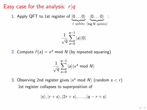
Easy case for the analysis: r |q1. Apply QFT to 1st register of |0 . . . 0i| {z }

` qubits

|0 . . . 0i| {z }dlogN qubitse

:

1pq

q�1X

a=0

|ai|0i

2. Compute f (a) = xa mod N (by repeated squaring)

1pq

q�1X

a=0

|ai|xa mod Ni

3. Observing 2nd register gives |x s mod Ni (random s < r)

1st register collapses to superposition of

|si, |r + si, |2r + si, . . . , |q � r + si

19/ 37

Easy case: r |q (continued)

Recall: 1st register is in superposition

q/r�1X

j=0

|jr + si

4. Apply QFT once more:

q/r�1X

j=0

q�1X

b=0

e2⇡i(jr+s)b

q |bi =q�1X

b=0

e2⇡isbq

0

@q/r�1X

j=0

⇣e2⇡i

rbq

⌘j

1

A

| {z }geometric sum

|bi

Sum 6= 0 i↵ e2⇡irbq = 1 i↵

rb

qis an integer

Only the b that are multiples ofq

rhave non-zero amplitude!

20/ 37

Easy case: r |q (continued)

5. Observe 1st register: random multiple b = cq

r, c 2 [0, r):

b

q=

c

r

I b and q are known; c and r are unknown

I c and r are coprime with probability � 1/ log log r

I Then: we find r by writingb

qin lowest terms

I Since we can find r , we can find prime factors of N !

Hard case (r 6 |q) still works approximately: measurement gives

b s.t.b

q⇡ c

r; we can find r with some extra number theory

21/ 37

Summary for Shor’s algorithm

I Reduce factoring to finding the period r of modularexponentiation function f (a) = xa mod N

I Use quantum Fourier transform to find a multiple of q/r ,repeat a few times to find r

I Overall complexity:

I QFT takes O(log q)2 = O(logN)2 elementary gatesI Modular exponentiation: ⇡ (logN)2 log logN gates;

classical computation by repeated squaring(use Schonhage-Strassen algo for fast multiplication)

I Everything repeated O(log logN) timesI Classical postprocessing takes O(logN)2 gates

I Roughly (logN)2 elementary gates in total

22/ 37

The search problem

I We want to search for some good item inan unordered N-element search space

I Model this as function f : {0, 1}n ! {0, 1} (N = 2n)f (x) = 1 if x is a solution

I We can query f :Of : |xi|0i 7! |xi|f (x)iorOf : |xi 7! (�1)f (x)|xi

I Goal: find a solution

I Classically this takes O(N) steps (queries to f )

I Grover’s algorithm does it in O(pN) steps

23/ 37

Grover’s algorithm

I Apply Grover iteration G k times on uniform starting state

8>>>><

>>>>:

n

|0i

|0i

|0i

9>>>>=

>>>>;

measure

H

H

H

G G

. . .

. . .

. . .

G

| {z }k

I Idea: each iteration moves amplitude towards solutions

24/ 37

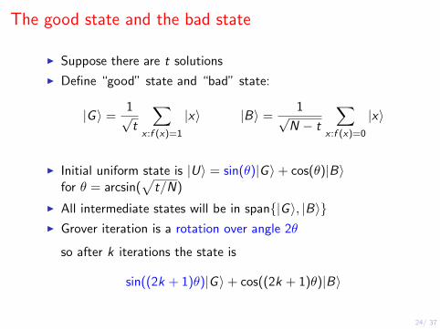
The good state and the bad state

I Suppose there are t solutions

I Define “good” state and “bad” state:

|G i = 1pt

X

x :f (x)=1

|xi |Bi = 1pN � t

X

x :f (x)=0

|xi

I Initial uniform state is |Ui = sin(✓)|G i+ cos(✓)|Bifor ✓ = arcsin(

pt/N)

I All intermediate states will be in span{|G i, |Bi}I Grover iteration is a rotation over angle 2✓

so after k iterations the state is

sin((2k + 1)✓)|G i+ cos((2k + 1)✓)|Bi

25/ 37

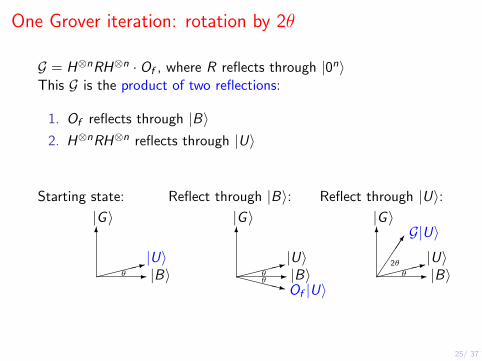
One Grover iteration: rotation by 2✓

G = H⌦nRH⌦n · Of , where R reflects through |0niThis G is the product of two reflections:

1. Of reflects through |Bi2. H⌦nRH⌦n reflects through |Ui

Starting state: Reflect through |Bi: Reflect through |Ui:

|Bi

|G i

✓

|Ui6

-⇠⇠⇠⇠: |Bi

|G i

✓✓

|Ui

Of |Ui

6

-⇠⇠⇠⇠:XXXXz

|Bi

|G i

✓2✓ |Ui

G|Ui6

-⇠⇠⇠⇠:⌦⌦⌦⌦�

26/ 37

How many iterations do we need?

I Success probability after k iterations:

sin2((2k + 1)✓), with ✓ = arcsin(p

t/N) ⇡pt/N

I If k =⇡

4✓� 1

2, then success probability is sin2(⇡/2) = 1

I Example: t = N/4 solutions ) k = 1

I In general, round k to nearest integer (incurs small error)

I Query complexity is k ⇡ ⇡

4

pN/t

This is optimal for a quantum algorithm!

I Gate complexity is O(pN/t logN)

27/ 37

Summary for Grover’s algorithm

I Quantum computers can search any N-element space witht = "N solutions, in O(

pN/t) = O(1/

p") iterations

1. Set up uniform starting state |Ui2. Repeat the following O(1/

p") times:

2.1 Reflect through |Bi (costs 1 query)

2.2 Reflect through |Ui (costs O(logN) gates)

3. Measure final state to obtain an index i

I If we don’t know " = t/N, we can try di↵erent guesses, stillfind a solution with expected number of O(1/

p") iterations

I The algorithm has a small error probability,but can be modified to error 0 if we know t exactly

28/ 37

Application: Speed up NP problems

I Given a propositional formula f (x1

, . . . , xn)Computable in time poly(n)

Question: is f satisfiable?

I This is a typical NP-complete problem

I Search space of N = 2n possibilities

I Classically: exhaustive search is the best we know.This takes about N steps

I Quantumly: Grover finds a satisfying assignment inpN · poly(n) steps

I Because Grover is optimal, we believe that NP-hard problemscannot be e�ciently computed by quantum algorithms

29/ 37

Classical random walks

I Explore a graph by moving torandom neighbor in each step

I If G is d-regular and connected: normalized adjacency matrixhas “spectral gap” � 2 (0, 1). Starting from any vertex,O(1/�) random walk steps produce uniform distribution

I Suppose an "-fraction of the vertices are “marked” and wewant to find such a marked vertex. Simple classical algorithm:

1. Start at random vertex v (setup cost S)

2. Do the following O(1/") times:

2.1 Check if v is marked (checking cost C)

2.2 Rerandomize v by O(1/�) RW steps (step cost U)

This finds marked item w.h.p. Cost is S+1

"

✓C+

1

�U

◆

30/ 37

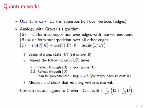
Quantum walks

I Quantum walk: walk in superposition over vertices (edges)

I Analogy with Grover’s algorithm:|G i = uniform superposition over edges with marked endpoint|Bi = uniform superposition over all other edges|Ui = sin(✓)|G i+ cos(✓)|Bi, ✓ = arcsin(1/

p")

1. Setup starting state |Ui (setup cost S)

2. Repeat the following O(1/p") times:

2.1 Reflect through |Bi (checking cost C)

2.2 Reflect through |Ui(can be implemented using 1/

p� QW steps, each at cost U)

3. Measure and check that resulting vertex is marked.

Correctness analogous to Grover. Cost is S+ 1p"

⇣C+ 1p

�U

⌘

31/ 37

Example: Ambainis’s algorithm (’03)

Suppose we want to find a collision in h : [n] ! N

I G =Johnson graph: the vertices are the sets R ✓ [n] of size r .Edge between sets R and R 0 if they di↵er in 1 element

I Fraction of vertices of G that contain collision: " � (r/n)2

I Known: spectral gap is � ⇡ 1/r

I With each vertex R , algorithm records h(R);setup cost S = r ; checking cost C = 0; update cost U = O(1)

I Total cost: S+1p"

✓C+

1p�U

◆r=n2/3= O(n2/3)

I Classically: ⇥(n) f -evaluations needed

If h is 2-to-1: run on random set ofpn inputs (whp 1 collision) to

get complexity O(n1/3)

Classically: ⇥(pn) f -evaluations, by birthday paradox

32/ 37

HHL algorithm for “solving” large linear systems

I Solving large linear systems Ax = b is one of the mostimportant problems in science and engineering.

Goal: given matrix A and vector b, find vector x

I Harrow-Hassidim-Lloyd’09: “solves” this problemexponentially faster by preparing state |xi IF

system is well-behaved:

Assumptions

(1) state |bi easy to prepare;

(2) A is well-conditioned: �max/�min not too big;

(3) unitary operation e iA is easy to apply (sparseness su�ces)

33/ 37

How does the Harrow-Hassidim-Lloyd algorithm work?

I Input: Hermitian matrix A 2 RN⇥N and vector b 2 RN

Goal: approximately prepare |xi, where Ax = b

I Let v1

, . . . , vN ,�1, . . . ,�N be eigenvectors, eigenvalues of A

I HHL algorithm:

1. Prepare quantum state |bi =PN

i=1

�i |vi iNB: applying A�1 corresponds to multiplying with ��1

i

2. Use eigenvalue estimation:PN

i=1

�i |vi i|�i i

3. Make new qubitPN

i=1

�i |vi i|�i i✓��1

i |0i+q1� ��2

i |1i◆

4. Uncompute |�i i by inverting eigenvalue estimation

5. Amplify the |0i-part to end withPN

i=1

�i��1

i |vi i = |xi

34/ 37

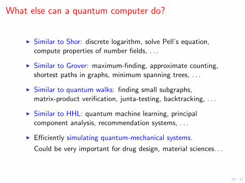
What else can a quantum computer do?

I Similar to Shor: discrete logarithm, solve Pell’s equation,compute properties of number fields, . . .

I Similar to Grover: maximum-finding, approximate counting,shortest paths in graphs, minimum spanning trees, . . .

I Similar to quantum walks: finding small subgraphs,matrix-product verification, junta-testing, backtracking, . . .

I Similar to HHL: quantum machine learning, principalcomponent analysis, recommendation systems, . . .

I E�ciently simulating quantum-mechanical systems.

Could be very important for drug design, material sciences. . .

35/ 37

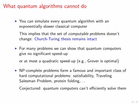
What quantum algorithms cannot do

I You can simulate every quantum algorithm with anexponentially slower classical computer

This implies that the set of computable problems doesn’tchange: Church-Turing thesis remains intact

I For many problems we can show that quantum computersgive no significant speed-up

or at most a quadratic speed-up (e.g., Grover is optimal)

I NP-complete problems form a famous and important class ofhard computational problems: satisfiability, TravelingSalesman Problem, protein folding,. . .

Conjectured: quantum computers can’t e�ciently solve them

36/ 37

Conclusion

I Quantum mechanics is the best physical theory we have

I Fundamentally di↵erent from classical physics:

superposition, interference, entanglement

I Quantum algorithms use these non-classical e↵ects to solvesome problems much faster

I We saw 4 important examples:

1. Shor’s factoring algorithm2. Grover’s search algorithm3. Ambainis’s collision-finding algorithm4. HHL algorithm for linear systems

Much more left to be discovered. . .

37/ 37

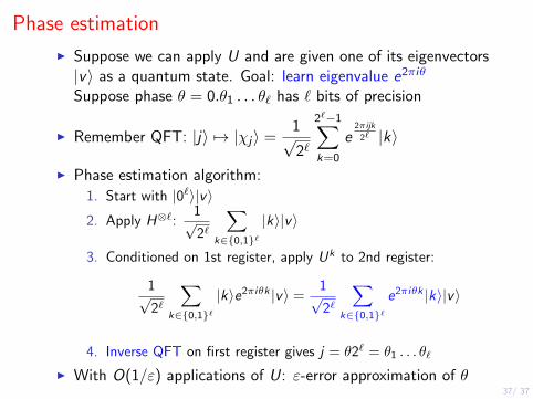
Phase estimation

I Suppose we can apply U and are given one of its eigenvectors|vi as a quantum state. Goal: learn eigenvalue e2⇡i✓

Suppose phase ✓ = 0.✓1

. . . ✓` has ` bits of precision

I Remember QFT: |ji 7! |�ji =1p2`

2

`�1X

k=0

e2⇡ijk

2

` |ki

I Phase estimation algorithm:1. Start with |0`i|vi2. Apply H⌦`:

1p2`

X

k2{0,1}`

|ki|vi

3. Conditioned on 1st register, apply Uk to 2nd register:

1p2`

X

k2{0,1}`

|kie2⇡i✓k |vi = 1p2`

X

k2{0,1}`

e2⇡i✓k |ki|vi

4. Inverse QFT on first register gives j = ✓2` = ✓1

. . . ✓`

I With O(1/") applications of U: "-error approximation of ✓

quantum algorithms tutorial - pqcrypto this tutorial: get to know your enemy! 3/ 37 quantum bits i...

Documents