Quantization of LPC Parameters

K.K. Paliwal and W.B. Kleijn

1. Introduction

Accurate reconstruction of the envelope of the short-time power spectrum is very important for

both the quality and intelligibility of coded speech. For low-bit-rate speech coding, the linear

predictive coding (LPC) parameters are widely used to encode the spectral envelope. The LPC

parameters form a perceptually attractive description of the spectral envelope since they describe

the perceptually important spectral peaks more accurately than the spectral valleys [1]. As a result,

the LPC parameters are used to describe the power spectrum envelope not only in LPC-based coders

(e.g. [2, 3]), but also in some coders which are based on entirely different principles (e.g. [4, 5]).

In speech coding applications, the LPC parameters are extracted frame-wise from the speech

signal, typically at the rate of 50 frames/sec. For telephone speech sampled at 8 kHz, typically a

10’th order LPC analysis is performed. The LPC parameters are quantized prior to their trans-

mission. Most commonly, memoryless quantizers using 20 to 40 bits are employed to encode the

LPC parameters at each frame update. Thus, the transmission of the (short-term) power-spectrum

envelope requires between 1 and 2 kb/s, which is a major contribution to the overall bit rate for

low-rate speech coders. It is, therefore, important to quantize these parameters using as few bits as

possible.

Considerable work has been done to develop both scalar and vector quantization procedures

for the LPC parameters. Scalar quantizers quantize each LPC parameter independently. Vector

quantizers consider the entire set of LPC parameters as an entity and allow for direct minimization

of quantization distortion. Because of this, the vector quantizers result in smaller quantization

distortion than the scalar quantizers at any given bit rate [6, 7]. Our aim in this chapter is to

provide an overview of scalar and vector quantization techniques proposed in the literature for

quantizing LPC parameters [8, 9, 10, 11, 12, 13, 14, 15, 16, 17, 18, 19, 20, 21, 22, 23, 24]. Since

results for these LPC quantization techniques have been reported in the literature on different data

bases, it is not possible to make meaningful comparisons about these techniques. Because of this,

we provide in this chapter results for these quantization techniques on a common data base. These

results are reported here in terms of a spectral distortion measure (which is used here as the criterion

for evaluating the quantization performance).

1

This chapter is organized as follows. In section , we discuss briefly the various methods of LPC

analysis and their merits. We discuss the evaluation of the performance of LPC quantizers in section

. In this section we introduce a commonly used spectral distortion criterion, which we will also use to

evaluate the various quantization procedures in the later sections. Section describes the speech data

base used in our experiments to study different LPC quantization techniques. In section we evaluate

scalar quantization techniques for LPC parameters, and in section we evaluate vector quantization

procedures. We attempt to find a lower limit for quantizing the LPC parameters in section . In

section we describe interpolation of LPC parameters and we summarize the chapter in section .

2. LPC analysis

It is common to distinguish two types of correlations in the speech signal: i) correlations over time

lags of less than 2 ms, the so-called short-term correlations and ii) correlations resulting from the

periodicity of the speech signal, which are observed over time lags of 2 ms or more and which are

called the long-term correlations. The short-term correlations determine the envelope of the power

spectrum and the long-term correlations determine the fine-structure of the power spectrum. Both

these correlations can be interpreted as a form of redundancy, and it is generally considered to be

beneficial to extract and encode these correlations as a first step in encoding the speech signal. The

LPC analysis described in this chapter captures the short-term correlations, and describes them in

the form of LPC parameters.

The short-term correlations observed in a segment of speech are a function of the shape of the

vocal tract. The rate at which the vocal tract changes is limited, and it has been found that an

update rate for the LPC parameters of about 50 Hz suffices for coding purposes. In this section, we

first briefly review the basic autocorrelation method for LPC analysis and then describe a number

of procedures which are aimed at obtaining improved analysis performance.

2.1. A brief review of basic LPC analysis

Consider a frame of speech signal having N samples, {s1, s2, . . . , sN}. In LPC analysis, it is assumed

that the current sample is approximately predicted by a linear combination of p past samples; i.e.,

sn = −

p∑

k=1

aksn−k, (1)

where p is the order of LPC analysis and {a1, . . . , ap} are the LPC coefficients. The value of p

typically is 10 for speech sampled at 8 kHz. Let en denote the error between the actual value and

2

the predicted value; i.e.,

en = sn − sn

= sn +

p∑

k=1

aksn−k. (2)

Since {en} is obtained by subtracting {sn} from {sn}, it is called the residual signal. The short-term

correlations between samples of the residual signal are low, and, therefore, the envelope of its power

spectrum will be approximately flat. Taking z transform of eq. 2, it follows that

E(z) = A(z)S(z), (3)

where S(z) and E(z) are the z transforms of the speech signal and the residual signal, respectively,

and

A(z) = 1 +

p∑

k=1

akz−k. (4)

The filter A(z) is known as the “whitening” filter as it removes the short-term correlation present

in the speech signal and, therefore, flattens the spectrum. Since E(z) has an approximately flat

spectrum, the short-time power-spectral envelope of the speech signal is modeled in LPC analysis

by an all-pole (or, autoregressive) model

H(z) = 1/A(z). (5)

The filter A(z) is also known as the “inverse” filter as it is the inverse of the all-pole model H(z) of

the speech signal.

In LPC analysis, the short-time power-spectral envelope of speech is obtained by evaluating H(z)

on the unit circle. However, for this, the LPC coefficients have to be computed first from the speech

signal. These are usually determined by minimizing the total-squared LPC error,

E =

n2∑

n=n1

e2n, (6)

where the summation range [n1, n2] depends on which of the two methods (the autocorrelation

method and the covariance method) is used for LPC analysis. These two methods are briefly

described below.

2.1.1. Autocorrelation method

In the autocorrelation method of LPC analysis, the summation range is [−∞,∞] which means that

the speech signal has to be available for all time. For short-time LPC analysis, this can be achieved

3

by windowing the speech signal and assuming the samples outside this window to be zero. For

windowing, tapered cosine window functions (such as the Hamming and Hanning window functions)

are preferred over the rectangular window function and the speech signal is multiplied by one of

these window functions prior to its LPC analysis. In this case, minimization of the error criterion

defined in eq. 6 leads to the following equations:

p∑

k=1

r|i−k|ak = −ri, 1 ≤ i ≤ p, (7)

where rk is the kth autocorrelation coefficient of the windowed speech signal and is given by

rk =1

N

N∑

n=k

wnsnwn−ksn−k. (8)

Here {wi} is the window function, which is of duration N samples.

The p equations defined by eq. 7 are called the Yule-Walker equations and have to be solved to

obtain p LPC coefficients. These equations can be written in the matrix form as follows:

Ra = −r, (9)

where

R =

r0 r1 r2 · · · rp−1

r1 r0 r1 · · · rp−2

r2 r1 r0 · · · rp−3

......

.... . .

...rp−1 rp−2 rp−3 · · · r0

, (10)

a = [a1, a2, . . . , ap]T , (11)

and

r = [r1, r2, . . . , rp]T . (12)

Here, the superscript T indicates the transpose of a vector (or matrix).

The matrix R (eq. 10) is often called the autocorrelation matrix. It has a Toeplitz structure.

This facilitates the solution of the Yule-Walker equations (eqs. 7, 9) for the LPC coefficients {ai}

through computationally fast algorithms such as the Levinson-Durbin algorithm [26, 27] and the

Schur algorithm [28, 29]. The Toeplitz structure guarantees the poles of the LPC synthesis filter

H(z) to be inside the unit circle. Thus, the synthesis filter H(z) resulting from the autocorrelation

method will always be stable. This is a major motivating factor for using the autocorrelation method

for LPC analysis.

4

2.1.2. Covariance method

In the covariance method of LPC analysis, the summation range is [p + 1, N ]. Therefore, there is

no windowing required here. Minimization of the total-squared-error, E, results in the following p

normal equations:

p∑

k=1

cikak = −ci0, 1 ≤ i ≤ p, (13)

where

cik =

N∑

n=p+1

sn−isn−k. (14)

The p normal equations (13) can be written in matrix form as follows:

Ca = −c, (15)

where

C =

c11 c12 c13 · · · c1p

c21 c22 c23 · · · c2p

c31 c32 c33 · · · c3p

......

.... . .

...cp1 cp2 cp3 · · · cpp

, (16)

c = [c10, c20, . . . , cp0]T . (17)

The matrix C is commonly called the covariance matrix. Since cik = cki, it is a symmetric matrix.

However, it does not have a Toeplitz structure. Because of this, the p normal equations (eqs. 13,15)

for LPC coefficients can not be solved as efficiently as in the autocorrelation method. The symmetric

structure of covariance matrix C can be exploited to derive some computationally fast algorithms

[27], though these are not as fast as the Levinson-Durbin and Schur algorithms. It may be noted that

the LPC coefficients estimated by the covariance method do not always result in a stable synthesis

filter H(z). Some procedures have been reported in the literature [30] which modify the covariance

method so that the estimated synthesis filter is always stable. However, this is done at the expense

of introducing additional error in the estimation of LPC coefficients.

2.2. Improvements and alternatives for LPC analysis

LPC analysis works under the assumption that speech can be modeled as the output of an all-pole

filter H(z) (defined by eq. 5). Excitation to this filter is assumed to be either a single impulse

(for voiced speech) or a white random noise sequence (for unvoiced speech). In practice, these

assumptions are not exactly valid for the observed speech signal (especially for voiced speech). As

5

a result, the LPC coefficients estimated by means of the autocorrelation method (or the covariance

method) contain a certain amount of error. Furthermore, the analysis method tends to be sensitive

to numerical errors when the analysis procedure is implemented on devices of limited precision, such

as fixed-point digital signal processors (DSPs). In this subsection, we discuss some of these problems

and improvements introduced to address these problems.

2.2.1. Methods aimed at periodic excitation in voiced speech

The LPC analysis technique is based on the assumption that the excitation source is either a single

impulse or a white random noise. Obviously, this assumption is not valid for the voiced sounds where

the excitation source is a pulse train of certain pitch period. Because of this, the speech samples

near pitch pulses are not predicted well and the residual error signal {en} is relatively large in the

neighborhood of these pitch pulses. This affects the estimation accuracy of LPC analysis [31, 32].

One approach to overcome this limitation is to use pitch-synchronous analysis over the glottal-

closure interval [33, 34]. However, detection of the glottal-closure interval is a difficult and com-

putationally expensive task. In addition, this approach fails to estimate the system parameters

correctly for the voiced sounds of female speakers where the pitch period is rather short and the

number of samples in the glottal-closure interval is very small. These problems can be overcome by

using the sample-selective LPC analysis technique [35] which is pitch-asynchronous in nature and

uses only those samples from the 20-40 ms speech frame which correspond to zero excitation. A

related method is proposed by Lee [36], where portions of the residual signal near the pitch pulses

are de-emphasized prior to its minimization using the criterion defined by eq. 6. Another approach

to overcome this limitation is to use an estimate of excitation pulse train to compute the parameters

of the all-pole filter [37, 38].

2.2.2. Lag windows and bandwidth widening

LPC analysis has problems in estimating accurately the spectral envelope for high-pitch voiced

speech sounds. The spectral information about a periodic signal is contained only at harmonics. For

high-pitched voices, the harmonic spacing is too large to provide an adequate sampling of the spectral

envelope. For this reason, LPC analysis does not provide accurate estimation of spectral envelope

for female speakers. Such inaccurate estimation occurs mainly in formant bandwidths which tend to

be underestimated by a large amount. This may result in unnatural (metallic sounding) synthesized

speech.

Two procedures have proven popular to overcome this problem of bandwidth underestimation.

6

In the first procedure [39], the autocorrelations are multiplied by a so-called lag window. Usually,

this lag window is chosen to have a Gaussian shape. This corresponds to convolving the power

spectrum with a Gaussian shape, widening the peaks of the spectrum. The second procedure is the

use of bandwidth widening [40]. In this procedure, each LPC coefficient an is multiplied by a factor

γn (i.e., all an are replaced by γnan). Such a multiplication moves all the poles of H(z) inward by

a factor γ and causes bandwidth expansion for all the poles. Let vi be the radius of ith pole, then

the bandwidth of this pole is defined as

Bi = −1

πTln(vi), (18)

where T is the sampling interval. A multiplication of the radius by γ expands this bandwidth to

Bi + ∆B, where

∆B = −1

πTln(γ). (19)

Note that this procedure expands the bandwidths of all the poles of H(z) by the same amount.

Bandwidth widening is now commonly used in speech coders; typical values for γ are between

0.988 and 0.996 [39], corresponding to between 10 and 30 Hz widening. While not as common as

bandwidth widening, lag windows are also used in many coders. Both procedures are independent

of the actual estimation procedure used for the LPC parameters.

2.2.3. Methods aimed at reducing the frame-to-frame fluctuations

In pitch-asynchronous LPC analysis procedures, LPC analysis frames are located arbitrarily with

respect to the pitch pulses, resulting in a considerable amount of frame-to-frame variation in the

estimated LPC coefficients [41]. This may cause some roughness in the quality of coded speech, which

increases when the LPC analysis interval is reduced. Because of this, it is desirable to estimate the

LPC coefficients in such a manner that they evolve smoothly over frames.

One approach to overcome this problem is to locate LPC analysis windows in such a manner that

they are always placed similarly relative to the pitch pulses. This approach has been used in some

speech coders such as the U.S. Federal Standard 1015 (also known as LPC10e). Another approach

to obtain smooth frame-to-frame evolution of estimated LPC coefficients is to multiply the residual

error signal en in eq. 6 by a tapered window function prior to its minimization [41].

2.2.4. Methods aimed at pole-zero modeling of speech

Since the LPC analysis technique assumes the speech-generating system to be an all-pole filter, its

estimation accuracy gets worse if there exist, in addition to poles, some zeros in the system transfer

7

function as is the case with the nasal and fricative sounds. Also, in the case of noisy speech, the

additive noise may introduce zeros in the spectrum and the performance of the all-pole LPC analysis

technique gets affected drastically.

To overcome this limitation, a reasonable approach is to extend the all-pole model to a pole-

zero model. Pole-zero modeling is a difficult problem as estimation of its parameters requires the

solution of nonlinear equations [42]. However, there are a number of efficient but sub-optimal

techniques available for estimating the parameters of the pole-zero model [43, 44, 45, 46, 37, 47].

These techniques can be used for pole-zero modeling of nasal and fricative sounds.

For noisy speech, where estimation of only the all-pole part of the pole-zero model is required,

some additional techniques have been proposed in the literature [48, 49] which use both low- and

high-order Yule-Walker equations for estimating the LPC coefficients. Some improvement using

these methods is claimed, but these procedures have not been tested for large data bases, are

computationally complex, and do not guarantee that H(z) is stable.

Another method [50] to obtain robust estimates for the LPC parameters from noisy speech signal

is based on multi-taper analysis [51]. This method uses a plurality of (orthogonal) windows. Each

of these windows can provide an independent estimate of the autocorrelation coefficients or of the

LPC parameters themselves. These independent estimates can then be averaged to obtain a robust

estimate.

2.2.5. Methods to improve numerical robustness

Due to the -6 dB/octave spectral tilt arising from the triangular shape of the excitation signal and

radiation effects. the speech spectrum shows a large dynamic range. This spectral dynamic range is

further increased due to the low-pass filtering used prior to the analog-to-digital conversion process.

This filtering makes the high frequency components in the speech spectrum (near half the sampling

frequency) very low in amplitude. As a result, LPC analysis requires high computational precision

to capture the description of features at the high end of the spectrum. More importantly, when these

features are very small, the autocorrelation or covariance matrices can become singular, resulting in

computational problems.

Application of the lag window described earlier in this section minimizes the dynamic range of

the spectrum by reducing its peaks. Since this is done prior to the solution for the LPC parameters,

it results in better numerical properties.

By adding to the original signal a low-level high-frequency noise, the dynamic range of the

power spectrum is reduced [52, 30]. It is convenient to add such a contribution directly to the

8

autocorrelation matrix for the autocorrelation method (or the corresponding covariance matrix for

the covariance method). This so-called high-frequency correction substantially reduces numerical

problems in computational devices of limited precision. The procedure is often simplified to be

a white-noise correction. This entails simply adding a small value to the diagonal samples of the

autocorrelation matrix.

3. Objective criteria for evaluating LPC quantization perfor-

mance

An important aspect in the design of an LPC quantizer is its evaluation. Ideally, the usefulness

of an LPC quantizer should be judged by means of subjective listening tests using human test

subjects. There are two reasons for not doing so: i) it is impossible to define a testing setup which

is independent of a particular coding or analysis-synthesis system, and ii) formal human listening

tests are time-consuming and expensive.

Thus, the evaluation of an LPC quantization procedure is usually performed using an objective

measure. A proper criterion should be based on the properties of human hearing. Furthermore, it

would seem reasonable that the criterion be consistent with the criterion used for the determination

of LPC parameters in the first place. However, as will be explained below, for the commonly used

criterion for evaluating the performance of LPC parameter quantization, neither of these conditions

are satisfied.

The criterion used for the computation of the LPC parameters is minimization of the residual

signal energy. This corresponds to a somewhat ad-hoc criterion in the spectral domain. Probably for

this reason, the minimization of the residual has not been adopted for evaluating the performance

of quantizers for the LPC parameters.

Objective measures for spectral fidelity can be defined on the basis of the understanding of the

human auditory systems [53, 54, 55, 56]. Such measures should account for spectral masking and

the fact that human hearing has a frequency resolution which is highly nonlinear (e.g. see [57]).

Despite these efforts towards a proper objective measure, a simple spectral distortion measure

is commonly used in the literature (e.g. [10, 11, 12, 13, 14, 15, 16, 17, 18, 19, 20, 21, 22, 23, 24])

For compatibility reasons, we will use the same simple measure in our study of LPC quantizer per-

formance in the following sections. In this section, we define this measure and comment about its

usefulness in demarking “transparent” quantization of LPC parameters. By “transparent” quanti-

zation of LPC parameters, we mean that the LPC quantization does not introduce any additional

audible distortion in the coded speech; i.e., the two versions of coded speech — the one obtained by

9

using unquantized LPC parameters and the other by using the quantized LPC parameters — are

indistinguishable through listening.

The common spectral distortion measure for a frame i is defined (in dB) as follows:

Di =

√

1

Fs

∫ Fs

0

[10 log10(Pi(f)) − 10 log10(Pi(f))]2df, (20)

where Fs is the sampling frequency in Hz, and Pi(f) and Pi(f) are the LPC power spectra of the

i-th frame given by

Pi(f) = 1/|Ai(exp(j2πf/Fs))|2, (21)

and

Pi(f) = 1/|Ai(exp(j2πf/Fs))|2, (22)

where Ai(z) and Ai(z) are the original (unquantized) and quantized LPC polynomials, respectively,

for the i-th frame. The spectral distortion is evaluated for all frames in the test data and its

average value is computed. This average value represents the distortion associated with a particular

quantizer.

As mentioned before, the average spectral distortion has been used extensively in the past to

measure the performance of LPC parameter quantizers. Earlier studies [10, 13, 14, 15] have used an

average spectral distortion of 1 dB as difference limen for spectral transparency. However, it has been

observed [16] that too many outlier frames in the speech utterance having large spectral distortion

can cause audible distortion, even though the average spectral distortion is 1 dB. Therefore, the

more recent studies [16, 17, 18] have tried to reduce the number of outlier frames, in addition to the

average spectral distortion.

In the next sections, we follow reference [16] and compute the spectral distortion in the 0-3

kHz band, and define a frame to be an outlier frame if it has a spectral distortion greater than 2

dB. The outlier frames are divided into the following two classes: i) outlier frames having spectral

distortion in the range 2-4 dB, and ii) outlier frames having spectral distortion greater than 4 dB.

We have observed that we can achieve transparent quantization of LPC parameters if we maintain

the following three conditions: i) the average distortion is about 1 dB, ii) there is no outlier frame

having spectral distortion larger than 4 dB, and iii) the number of outlier frames having spectral

distortion in the range 2-4 dB is less than 2%. Note that transparent quantization of LPC parameters

may be possible with a higher number of outlier frames, but we have not investigated it.

10

4. Data base

As mentioned earlier, different LPC quantization techniques are evaluated in the literature on dif-

ferent data bases and, hence, it is not possible to compare them meaningfully. As our aim in the

present chapter is to review these techniques and to put their performance in a proper perspective,

we evaluate them on a common data base. In this section, we describe this data base.

The speech data base used in our experiments consists of 23 minutes of speech recorded from 35

different FM radio stations. The first 1200 seconds of speech (from about 170 speakers) is used for

training, and the last 160 seconds of speech (from 25 speakers, different from those used for training)

is used for testing. The speech is low-pass filtered at 3.4 kHz and digitized at a sampling rate of 8

kHz. A 10’th order LPC analysis, based on the stabilized covariance method with high-frequency

compensation [52] and error weighting [41] (see section ), is performed every 20 ms using a 20-ms

analysis window. Thus, we have here 60000 LPC vectors for training, and 8000 LPC vectors for

testing. We will refer to this data base as the ‘FM radio’ data base. To avoid sharp spectral peaks

in the LPC spectrum, a 10 Hz bandwidth expansion is applied (i.e. γ = 0.996, see section ).

5. Scalar quantization of LPC parameters

A number of scalar quantization techniques have been reported in the literature for quantizing the

LPC parameters. These techniques quantize individual parameters separately, using either uniform

or nonuniform quantizers. Since nonuniform quantizers result in less quantization distortion than

uniform quantizers, we only report here results for nonuniform quantizers. These quantizers are

designed from the training data set of the FM data base using the Lloyd algorithm [58], which

is identical to the Linde-Buzo-Gray (LBG) algorithm [59] applied to individual LPC parameters.

The resulting quantizers are then evaluated on the test data set using spectral distortion as the

performance measure.

In speech-coding applications, it is necessary to quantize the LPC parameters with as little

distortion as possible. Also, it is required that the all-pole filter remains stable after quantization

of the LPC parameters. Direct scalar quantization of the LPC coefficients is usually not done as

small quantization errors in the individual LPC coefficients can produce relatively large spectral

errors and can also result in instability of the all-pole filter H(z). As a result, it is necessary to

use a relatively large number of bits to perform transparent quantization of LPC parameters by

quantizing the LPC coefficients {an} themselves. Using 6 bits/coefficient/frame (i.e., 60 bits/frame)

for the scalar quantization of the LPC coefficients in the FM data base, we found that 25.5% of

11

the frames result in unstable all-pole filters. This 60-bit quantizer resulted in an average spectral

distortion (according to eq. 20) of 1.83 dB.

Because of these problems, it is necessary to transform the LPC coefficients to other repre-

sentations which ensure stability of the all-pole filter after LPC quantization. In addition, these

representations should have one-to-one mapping; i.e., it should be possible to transform from one

representation to another without loosing any information about the all-pole filter. In the liter-

ature, a number of such representations have been proposed. These are the reflection coefficient

(RC) representation, the arcsine reflection coefficient (ASRC) representation, the log-area ratio

(LAR) representation and the line spectral frequency (LSF) representation. We describe below

scalar quantization of LPC parameters in terms of these representations.

5.1. Scalar quantization using the reflection coefficients

The reflection coefficients (RCs) can be obtained from the LPC coefficients using the Levinson-

Durbin recursion relations [27]. These coefficients have two major advantages over the LPC co-

efficients: i) they are spectrally less sensitive to quantization than the LPC coefficients, and ii)

the stability of the all-pole filter can be easily ensured by keeping each reflection coefficient within

the range −1 to +1 during the quantization process. Thus, these coefficients are more suitable for

quantization than the LPC coefficients.

Table 1: Spectral distortion (SD) performance of an RC-based scalar quantizer as a function of bitrate using uniform bit allocation.

Bits Av. SD Outliers (in %)used (in dB) 2-4 dB >4 dB50 0.59 2.39 0.0940 1.07 9.20 0.7430 1.93 30.96 6.40

Table 2: Spectral distortion (SD) performance of an RC-based scalar quantizer as a function of bitrate using nonuniform bit allocation.

Bits Av. SD Outliers (in %)used (in dB) 2-4 dB >4 dB36 0.88 2.49 0.0534 1.02 3.94 0.0932 1.16 6.69 0.1430 1.31 10.53 0.3028 1.42 13.93 0.5026 1.67 21.68 1.8624 1.93 32.80 3.66

We have studied the scalar quantization of LPC parameters in terms of RCs on the FM data base.

12

Since different RCs contribute differently to the average spectral distortion performance, it is not

advisable to use an equal number of bits for the quantization of different RCs. In our experiments,

we have used an integer bit allocation scheme which assigns, for a given bit rate per frame, different

number of bits to individual RCs as follows. Start from 0 bit/frame where zero bit is allocated

to every RC. Then for 1 bit/frame, the extra bit is assigned to the RC which gives the maximum

marginal improvement in the quantization performance. This procedure is repeated for the higher

bit rates until the required bit rate is reached. Obviously, this procedure will allocate a nonuniform

number of bits to individual RCs. To show the advantage of this nonuniform bit allocation procedure,

we report here the spectral distortion results with uniform as well as nonuniform bit allocation

schemes. These results are shown in tables 1 and 2, respectively. We can see from these tables

that the nonuniform bit allocation scheme offers a saving of about 6 bits/frame with respect to the

uniform bit allocation scheme.

It is seen that about 40 bits/frame are required to get an average spectral distortion of 1 dB using

RCs with uniform bit allocation, and about 34 bits/frame using nonuniform bit allocation. Since

the nonuniform bit allocation scheme results in better performance than the uniform bit allocation

scheme, we use it hereafter with all the scalar quantizers described in this chapter.

5.2. Scalar quantization with log-area ratios and arcsine reflection coeffi-

cients

Though the reflection coefficients are spectrally less sensitive to quantization distortion than the

LPC coefficients, they have the drawback that their spectral sensitivity curves are U-shaped, having

large values whenever the magnitude of these coefficients is close to unity. This means that these

coefficients are very sensitive to quantization distortion when they represent narrow-bandwidth poles.

However, this drawback can be overcome by the use of an appropriate nonlinear transformation

which expands the region near | Ki |= 1, where Ki is the i-th reflection coefficient. Two such

transformations are the log-area ratio transformation [8] and the inverse-sine transformation [9].

The log-area ratios (LARs), {L1, . . . , Lp}, are defined as

Li = log1 + Ki

1 − Ki, (23)

and the arcsine reflection coefficients (ASRCs), {J1, . . . , Jp}, are defined as

Ji = sin−1 Ki. (24)

We have studied scalar quantization of LPC parameters using the LAR and ASRC representa-

tions. The results are shown in tables 3 and 4, respectively. By comparing these tables with table 2,

13

Table 3: Spectral distortion (SD) performance of an LAR-based scalar quantizer as a function of bitrate.

Bits Av. SD Outliers (in %)used (in dB) 2-4 dB >4 dB36 0.80 1.09 0.0434 0.92 1.65 0.0432 1.04 3.20 0.0430 1.21 6.40 0.1128 1.34 9.51 0.1626 1.50 14.26 0.7124 1.75 25.93 1.59

Table 4: Spectral distortion (SD) performance of an ASRC-based scalar quantizer as a function ofbit rate.

Bits Av. SD Outliers (in %)used (in dB) 2-4 dB >4 dB36 0.81 0.90 0.0134 0.92 2.05 0.0832 1.04 3.30 0.0930 1.18 5.45 0.0928 1.32 9.29 0.2326 1.51 15.51 0.7124 1.75 26.13 1.49

it can be seen that the LAR and ASRC representations offer a saving of about 2 bits/frame over the

RC representations. The LAR and ASRC representations require about 32 bits/frame for providing

an average spectral distortion of 1 dB.

5.3. Scalar quantization using the LSF representation

The line spectrum frequency (LSF) representation was introduced by Itakura [60]. The LSF rep-

resentation has a number of properties, including a bounded range, a sequential ordering of the

parameters and a simple check for the filter stability, which makes it desirable for the quantization

of LPC parameters. In addition, the LSF representation is a frequency-domain representation and,

hence, can be used to exploit certain properties of the human perception system.

To define the LSFs, the inverse filter polynomial is used to construct two polynomials,

P (z) = A(z) + z−(M+1)A(z−1), (25)

and

Q(z) = A(z) − z−(M+1)A(z−1). (26)

The roots of the polynomials P (z) and Q(z) are called the LSFs. The polynomials P (z) and Q(z)

have the following two properties: i) all zeros of P (z) and Q(z) lie on the unit circle, ii) zeros of

14

P (z) and Q(z) are interlaced with each other; i.e., the LSFs are in ascending order. It can be shown

[10] that A(z) is minimum-phase if its LSFs satisfy these two properties. Thus, the stability of LPC

synthesis filter (which is an important pre-requirement for speech coding applications) can be easily

ensured by quantizing the LPC parameters in LSF domain.

A cluster of (2 or 3) LSFs characterizes a formant frequency and the bandwidth of a given

formant depends on the closeness of the corresponding LSFs. The spectral sensitivities of LSFs

are localized; i.e., a change in a given LSF produces a change in the LPC power spectrum only in

its neighborhood. Interpretation of LSFs in terms of formants makes them suitable for exploiting

certain properties of the human auditory system for LPC quantization. The localized spectral-

sensitivity property of LSFs makes them ideal for scalar quantization as the individual LSFs can

be quantized independently without significant leakage of quantization distortion from one spectral

region to another.

We have studied scalar quantization of LPC parameters in terms of LSFs on our FM data base.

Results are shown in table 5. It can be seen from this table that LSFs require about 34 bits/frame

for providing a 1dB average spectral distortion. Thus, straightforward scalar quantization of the

LSF provides a performance similar to that of the reflection coefficients.

Table 5: Spectral distortion (SD) performance of an LSF-based scalar quantizer as a function of bitrate.

Bits Av. SD Outliers (in %)used (in dB) 2-4 dB >4 dB36 0.79 0.46 0.0034 0.92 1.00 0.0132 1.10 2.21 0.0330 1.22 4.88 0.0328 1.40 9.21 0.0526 1.58 16.96 0.0624 1.88 35.10 0.49

To exploit the correlation between successive LSFs, Soong and Juang [10] have advocated dif-

ferential quantization of LSFs; i.e. quantization of the differences between successive LSFs. We

have used the LSF differences (LSFDs) for scalar quantization of LPC parameters on our FM data

base. Results are shown in table 6. These results show that an average spectral distortion of 1 dB

can be obtained with the LSFDs using about 32 bits/frame (which amounts to a saving of about 2

bits/frame with respect to LSFs themselves).

Note that we have used the LBG algorithm for the design of scalar quantizers. This algorithm

takes into account nonuniform statistical distribution of individual LPC parameters, but gives only a

15

Table 6: Spectral distortion (SD) performance of an LSFD-based scalar quantizer as a function ofbit rate.

Bits Av. SD Outliers (in %)used (in dB) 2-4 dB >4 dB36 0.75 0.60 0.0134 0.86 1.10 0.0032 1.05 3.13 0.0130 1.17 5.94 0.0328 1.25 7.36 0.0526 1.45 12.46 0.2024 1.66 20.33 0.44

locally optimal design. Recently, Soong and Juang [14] have proposed a globally optimal design algo-

rithm which utilizes both nonuniform statistical distribution and spectral sensitivities of individual

LSFDs in the design procedure. We have used this algorithm on our FM data base to design scalar

quantizers for individual LSFDs. We have found that this algorithm does not show any significant

improvement over the LBG algorithm.

Quantization of LSFDs, due to its differential coding nature, occasionally leads to large spectral

distortions. This happens due to the so-called slope overload effect. When LSFDs to be quantized

exceed the full range of the quantizers, large spectral errors can occur. This problem can be overcome

by using delayed-decision coding. In the literature, the following two algorithms have been used for

delayed decision coding of LSFDs: the M-algorithm [18] and the A-star algorithm [17]. Both of

these algorithms use a Euclidean distance metric defined in terms of LSFs to find the optimal path.

However, since this Euclidean distance metric at times is a poor approximation to the spectral

distortion measure, the delayed decision coding of LSFDs can still have occasionally large spectral

errors. To overcome this problem, Soong and Juang [17] have suggested the use of a hybrid algorithm

where LSFDs are quantized directly (i.e., instantaneously) as well as with delayed decision coding,

and a choice between the two quantized versions of LSFDs is made using the spectral distortion

measure. We have used this hybrid algorithm for quantizing LPC parameters from the FM data

base. Using 30 bits/frame, we obtained an average spectral distortion of 1.06 dB, 1.11% frames

having spectral distortion in the range 2 to 4 dB, and 0.01% frame with spectral distortion greater

than 4 dB. By comparing these results with those shown in table 6, it can be observed that the

hybrid algorithm provides a saving of about 2 bits/frame over the direct quantization of LSFDs.

However, this improvement in quantization performance comes at the cost of a significant increase

in computational complexity.

It should be noted here that LPC quantization using the LSFD representation is more sensitive

16

to channel errors than in LPC quantization using the LSF representation [61]. Therefore, most

practical speech-coding systems use LSFs (e.g. [62]), despite the fact that quantization of the LSF

representation is inferior to quantization of the LSFD representation in terms of spectral distortion

performance.

6. Vector quantization of LPC parameters

As mentioned earlier, vector quantizers consider the entire set of LPC parameters as an entity and

allow for direct minimization of quantization distortion. Because of this, vector quantizers result in

a smaller quantization distortion than scalar quantizers [6, 7].

Juang et al. [19] have studied vector quantization of LPC parameters using the so-called likeli-

hood distortion measure [1] and shown that the resulting vector quantizer at 10 bits/frame is com-

parable in performance to a 24 bits/frame scalar quantizer. This vector quantizer at 10 bits/frame

has an average spectral distortion of 3.35 dB, which is not acceptable for practical speech coders.

For transparent quantization of LPC parameters, the vector quantizer needs more bits to quantize

one frame of speech. This means that the vector quantizer must have a large number of codevectors

in its codebook. Such a vector quantizer has the following two problems. Firstly, a large code-

book requires a prohibitively large amount of training data and the training process takes too much

computation time. Secondly, the storage and computational requirements for vector quantization

encoding is prohibitively high. Because of these problems, a sub-optimal vector quantizer has to be

used if transparent quantization of the LPC parameters is required.

To reduce the computational complexity and/or memory requirements, various forms of subop-

timal vector quantizers have been proposed [6, 7]. Best known among these are the tree-search and

product-code vector quantizers. In the literature, some studies have been reported for LPC quanti-

zation using these reduced complexity sub-optimal vector quantizers. For example, Paliwal and Atal

[22] have used a 2-stage vector quantizer and reported transparent quantization with 25 bits/frame.

Moriya and Honda [20] have used a hybrid vector-scalar quantizer (having a vector quantizer in the

first stage and a scalar quantizer in the second stage). This quantizer can give an average spectral dis-

tortion of about 1 dB using 30-32 bits/frame. Shoham [21] has proposed a cascaded vector quantizer

(which is a type of product-code vector quantizer) for LPC quantization. In this vector quantizer,

the LPC polynomial is decomposed into two lower-order polynomials. The decomposition is done

by finding the roots of the LPC polynomial, with 6 lower-frequency roots defining one polynomial

and the other 4 higher-frequency roots defining another polynomial. The resulting lower-order LPC

17

vectors are jointly quantized in an iterative fashion using the likelihood-ratio distance measure. This

cascaded vector quantizer has been shown to provide an average spectral distortion of 1.1 dB using

26 bits/frame for LPC quantization [21]. Another type of product-code vector quantizer, namely the

split vector quantizer, has been studied in [22, 24]. This vector quantizer can perform transparent

quantization of LPC parameters with 24 bits/frame [22]. Some of these suboptimal vector quantizers

are described below 1.

6.1. Multi-stage vector quantization of LPC parameters

The multi-stage vector quantizer is a type of product-code vector quantizer [6, 7]. It reduces the

complexity of a vector quantizer, but at the cost of lower performance. In this section, we study the

use of the 2-stage vector quantizer for LPC quantization and briefly describe the results.

In 2-stage vector quantization [22], the LPC parameter vector (in some suitable representation

such as the LSF representation) is quantized by the first-stage vector quantizer and the error vector

(which is the difference between the input and output vectors of the first stage) is quantized by

the second-stage vector quantizer. The final quantized version of the LPC vector is obtained by

summing the outputs of the two stages. To minimize the complexity of the 2-stage vector quantizer,

the bits available for LPC quantization are divided equally between the two stages. For example,

for 24 bits/frame LPC quantization, each stage has a codebook with 4096 codevectors.

Selection of a proper distortion measure is the most important issue in the design and operation

of a vector quantizer. Since the spectral distortion (defined by eq. 20) is used here for evaluating

LPC quantization performance, ideally it should be used to design the vector quantizer. However,

it is very difficult to design a vector quantizer using this distortion measure. Therefore, simpler

distance measures (such as the Euclidean and the weighted Euclidean distance measures) between

the original and quantized LPC parameter vectors (in some suitable representation such as the LSF

representation) are used to design the LPC vector quantizer.

To find the best LPC parametric representation for the Euclidean distance measure, we study the

2-stage vector quantizer with this distance measure in the following three domains: the LSF domain,

the arcsine reflection coefficient domain and the log-area ratio domain. Results for the 24 bits/frame

2-stage vector quantizer are shown in table 7 . It can be seen from this table that the 2-stage vector

quantizer performs better with the LSF representation than with the other two representations.

1Note that these vector quantizers are evaluated here on a homogeneous data base (described in section ), wheretraining and test conditions are similar. However, at times, the LPC vector quantizer have to be used in test conditionswhich are drastically different from training conditions (such as microphone and channel mismatches). In such cases,performance of these vector quantizers may deteriorate significantly [25]. However, we have not studied their LPCquantization performance under such drastically mismatched conditions.

18

Because of this, we will use hereafter the LSF representation for the vector quantization of LPC

parameters.

Table 7: Spectral distortion (SD) performance for 24 bits/frame 2-stage vector quantizers using theLSF, arcsine reflection coefficient (ASRC), and log-area ratio (LAR) representations (with Euclideandistance measure).

Para- Av. SD Outliers (in %)meter (in dB) 2-4 dB >4 dBLSF 1.23 6.71 0.04

ASRC 1.53 20.10 1.24LAR 1.33 11.71 0.55

As mentioned in section , different components of an LPC parameter vector have different spectral

sensitivities and, hence, a scalar quantizer using nonuniform bit allocation (which reflects different

spectral sensitivities of individual components) results in significantly better spectral distortion

performance than a scalar quantizer using uniform bit allocation. Similar reasoning applies to

vector quantizers. The Euclidean distance measure used for vector quantization in the preceding

section provides equal weights to individual components of the LSF vector, which obviously are

not proportional to their spectral sensitivities. In [22], Paliwal and Atal have proposed a weighted

Euclidean distance measure in the LSF domain which tries to assign weights to individual LSFs

according to their spectral sensitivities. The weighted Euclidean distance measure d(f , f) between

the test LSF vector f and the reference LSF vector f is given by

d(f , f) =

10∑

i=1

[ciwi(fi − fi)]2, (27)

where fi and fi are the i-th LSFs in the test and reference vector, respectively, and ci and wi are

the weights assigned to the i-th LSF. These are given by

ci =

1.0, for 1 ≤ i ≤ 8,0.8, for i = 9,0.4, for i = 10,

(28)

and

wi = [P (fi)]r, for 1 ≤ i ≤ 10, (29)

where P (f) is the LPC power spectrum associated with the test vector as a function of frequency

f and r is an empirical constant which controls the relative weights given to different LSFs and is

determined experimentally. A value of r equal to 0.15 was found to provide the best performance

for the criterion of eq. 20 in the present study. Note that the weights {wi} vary from frame-to-frame

depending on the LPC power spectrum, while the weights {ci} do not change from frame-to-frame

19

(i.e., they are fixed). These two weightings are called here the adaptive weighting and the fixed

weighting, respectively.

In the fixed weighting, the last two LSFs are assigned lower weights than the rest of the LSFs,

which takes into account the better resolving capability of the human ear for lower frequencies. In

the adaptive weighting, the weight assigned to a given LSF is proportional to the value of LPC

power spectrum at this LSF. Thus, this distance measure allows for quantization of LSFs in the

formant regions better than those in the non-formant regions. Also, the distance measure gives

more weight to the LSFs corresponding to the high-amplitude formants than to those corresponding

to the lower-amplitude formants; the LSFs corresponding to the valleys in the LPC spectrum get

the least weight. (Note that, whereas the fixed weighting improves the perceptual performance, it

does not necessarily improve the criterion of eq. 20.)

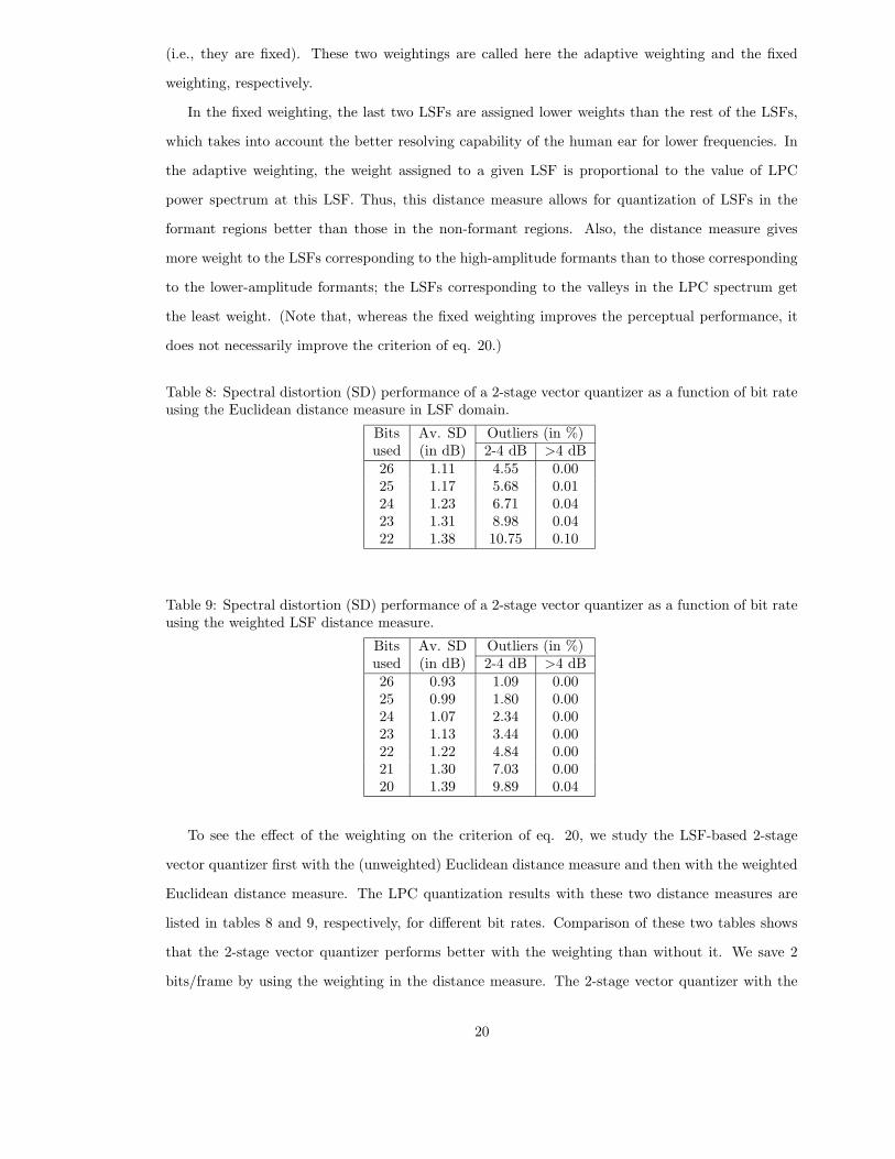
Table 8: Spectral distortion (SD) performance of a 2-stage vector quantizer as a function of bit rateusing the Euclidean distance measure in LSF domain.

Bits Av. SD Outliers (in %)used (in dB) 2-4 dB >4 dB26 1.11 4.55 0.0025 1.17 5.68 0.0124 1.23 6.71 0.0423 1.31 8.98 0.0422 1.38 10.75 0.10

Table 9: Spectral distortion (SD) performance of a 2-stage vector quantizer as a function of bit rateusing the weighted LSF distance measure.

Bits Av. SD Outliers (in %)used (in dB) 2-4 dB >4 dB26 0.93 1.09 0.0025 0.99 1.80 0.0024 1.07 2.34 0.0023 1.13 3.44 0.0022 1.22 4.84 0.0021 1.30 7.03 0.0020 1.39 9.89 0.04

To see the effect of the weighting on the criterion of eq. 20, we study the LSF-based 2-stage

vector quantizer first with the (unweighted) Euclidean distance measure and then with the weighted

Euclidean distance measure. The LPC quantization results with these two distance measures are

listed in tables 8 and 9, respectively, for different bit rates. Comparison of these two tables shows

that the 2-stage vector quantizer performs better with the weighting than without it. We save 2

bits/frame by using the weighting in the distance measure. The 2-stage vector quantizer with the

20

weighted LSF distance measure requires about 25 bits/frame to achieve transparent quantization of

LPC parameters (with an average spectral distortion of about 1 dB, less than 2% outliers in the

range 2-4 dB, and no outlier with spectral distortion greater than 4 dB).

6.2. Hybrid vector-scalar quantization of LPC parameters

The hybrid vector-scalar quantizer [20] is a 2-stage quantizer where the first stage is a vector quantizer

and the second stage is a scalar quantizer. This quantizer has less complexity than the 2-stage vector

quantizer. However, this complexity reduction comes at the cost of lower performance.

We have used this quantizer in the LSF domain to quantize LPC parameters from the FM data

base. Here, the vector quantizer which forms the first stage uses 8 bits/frame. The rest of the bits

are used by the second-stage scalar quantizer. Results from the vector-scalar quantizer are shown

in table 10. It can be seen from this table that this quantizer requires about 31-32 bits/frame for

transparent quantization of LPC parameters.

Table 10: Spectral distortion (SD) performance of a hybrid vector-scalar quantizer for different bitrates.

Bits Av. SD Outliers (in %)used (in dB) 2-4 dB >4 dB32 0.96 2.91 0.0031 1.02 3.78 0.0130 1.06 4.28 0.0128 1.18 6.19 0.0426 1.20 6.46 0.0424 1.36 11.13 0.10

6.3. Cascaded vector quantization of LPC parameters

The cascaded vector quantization [21] is a type of product-code vector quantization. Here, the LPC

polynomial is decomposed into two lower-order polynomials. The decomposition is done by finding

the roots of the LPC polynomial, with 6 lower-frequency roots defining one polynomial and the

other 4 higher-frequency roots defining another polynomial. The resulting lower-order LPC vectors

are jointly quantized in an iterative fashion using the likelihood ratio distance measure. We have

used this quantizer for the quantization of LPC parameters from the FM data base. Results are

shown table 11. It can be seen from this table that this quantizer does not provide transparent

quantization of LPC parameters with 26 bits/frame2.

2We have also studied the cascaded vector quantizer with LPC decomposition using 4 lower roots in the firstpolynomial and 6 higher roots in the other polynomial and obtained better results than the (6,4) decomposition, asused in [21]. For 24 bits/frame, the (4,6) decomposition results in an average spectral distortion of 1.21 dB, 3.90%outliers in the range 2-4 dB, and no outlier having distortion greater than 4 dB. However, these results are still inferiorto those obtained with the 24 bits/frame split vector quantizer.

21

Table 11: Spectral distortion (SD) performance of a cascaded vector quantizer for different bit rates.

Bits Av. SD Outliers (in %)used (in dB) 2-4 dB >4 dB26 1.29 5.06 0.0024 1.43 9.64 0.0622 1.60 17.21 0.08

.

6.4. Split vector quantization of LPC parameters

The split vector quantizer is another type of product-code vector quantizer which reduces the com-

plexity of a vector quantizer, but at the cost of lower performance. In split vector quantization

[22], the LPC parameter vector (in some suitable representation such as the LSF representation) is

split into a number of parts and each part is quantized separately using vector quantization. We

divide the LSF vector into two parts; the first part has the first four LSFs and the second part the

remaining 6 LSFs. For minimizing the complexity of the split vector quantizer, the total number of

bits available for LPC quantization are divided equally to individual parts. Thus, for a 24 bits/frame

LPC quantizer, each of the two parts is allocated 12 bits. We report here results for the 2-part split

vector quantizer on the FM data base. Results for split vector quantizer with more than two parts

are provided in [22].

Table 12: Spectral distortion (SD) performance of a split-vector quantizer as a function of bit rateusing Euclidean distance measure in the LSF domain.

Bits Av. SD Outliers (in %)used (in dB) 2-4 dB >4 dB26 1.05 2.23 0.0025 1.11 2.96 0.0124 1.19 4.30 0.0323 1.26 5.64 0.0422 1.34 8.06 0.05

Table 13: Spectral distortion (SD) performance of a split-vector quantizer as a function of bit rateusing the weighted LSF distance measure.

Bits Av. SD Outliers (in %)used (in dB) 2-4 dB >4 dB26 0.90 0.44 0.0025 0.96 0.61 0.0024 1.03 1.03 0.0023 1.10 1.60 0.0022 1.17 2.73 0.0021 1.27 4.70 0.0020 1.34 6.35 0.00

22

To see the effect of weighting on the Euclidean distance measure (see eq. 27), we study LPC

quantization using the unweighted as well as the weighted LSF-based Euclidean distance measures.

Results are shown in tables 12 and 13, respectively. It can be seen from these tables that transparent

quantization of LPC parameters can be performed by using about 26 bits/frame with unweighted

distance measure and 24 bits/frame with weighted distance measure. Similar to the 2-stage vector

quantizer, we save 2 bits/frame by using the weighting in the distance measure.

6.5. Other distortion measures for vector quantization of LPC parameters

As mentioned earlier, selection of a proper distortion measure is perhaps the most important issue

in the design of a vector quantizer. In the preceding subsections, we have used a weighted Euclidean

distance, defined in LSF domain by eq. 27, as the distortion measure. The weights in this distance

measure are derived from the LPC spectrum, using eq. 29. As argued in subsection , these weights

are consistent with the properties of the human auditory perception system. Note that this is not

the only choice of weights which is consistent with the human auditory perception properties. Other

choices are also possible. For example, Laroia et al. [24] have used the following weights:

wi =1

fi − fi−1+

1

fi+1 − fi, for 1 ≤ i ≤ 10. (30)

Here, f0 is set to zero and f11 to half of the sampling frequency. These weights can be justified

on human auditory perception considerations as the LSFs near formants are emphasized here, too.

We have studied the LPC quantization performance of the split vector quantizer using the weighted

Euclidean distance measure (eq. 27) with these weights. For 24 bits/frame, these weights result in

an average spectral distortion of 1.05 dB, 2.04% outliers in the range 2-4 dB, and 0.03% outliers

with spectral distortion greater than 4 dB. Comparing these results with the results shown in table

13, we can see that these weights do not perform as well as the weights given by eq. 29.

We have used spectral distortion (defined by eq. 20) as the criterion for evaluating the LPC

quantization performance. If our aim is to get best results in terms of this criterion, we should

ideally use the spectral distortion measure to design the LPC vector quantizer. However, it is

difficult to design a vector quantizer using the spectral distortion measure and, therefore, simpler

distance measures (such as the weighted Euclidean distance measure) are generally used. Recently,

some studies were reported [63, 64] where the spectral distortion is expressed in alternate forms

which can be easily used for the design of an LPC vector quantizer. In the LSF domain, the spectral

distortion measure translates to a form which is similar to the weighted Euclidean distance measure

(defined by eq. 27). The LPC quantization results obtained by this distortion measure are only

23

slightly better than those obtained by using the weighted Euclidean distance measure [63]. These

new methods can also be used during the search procedure of LSF vector quantizers, where they

can be used to obtain near-optimal weighting.

7. Estimating the minimum bit allocation required for LPC

parameters

In this section we make an attempt at estimating the lower limit for the number of bits required

for memoryless quantization of the LPC parameters at a 1 dB distortion (as defined by eq. 20). To

make the estimate, we assume that a set of LPC coefficient vectors, which are randomly selected

from a data base, form a reasonable codebook. An optimal codebook of similar size should perform

at least as well as such a randomly packed codebook, and, therefore, an estimate of the required size

for such a random codebook will form an upper bound for a properly optimized codebook.

Let us select a random set of LPC coefficient data points from a data base. Then we can select an

arbitrary point in the data base, and find how close this is to nearest point in this selected set (the

codebook). We selected a new codebook for each such trial and averaged over 100 nearest-neighbor

estimates. (We made sure that the nearest neighbor could not be the arbitrary point itself.) Figure

1 shows the resulting mean distances to the nearest codebook entry for the case where the randomly-

selected sets are of size 2 (1 bit) up to sets of 163840 (14 bits). It is seen that a 14-bit codebook can

be expected to perform well within 2 dB.

In practice, it is difficult to obtain a sufficient number of data points to obtain a situation

where the mean nearest-neighbor distance is within 1 dB (equivalent to transparent quantization).

Instead, we estimate the number of points required for this situation by means of extrapolation. This

extrapolation must be based on reasonable assumptions. First consider the fact that the spectra are

obtained from vectors of 10 LPC coefficients. Thus, these vectors must fall within a manifold within

the spectral space which must have an intrinsic dimensionality of 10 or less. Let us denote this

dimensionality to be k and consider a uniformly distributed set of points within this manifold. For

a sufficiently high density, the distance between adjacent points on the manifold and their density

f are related by

r(2) = αf1/k, (31)

where as distance, r(2), we have chosen the root-mean square distance and α is a constant. From

eq. 31, it can be concluded, that, for sufficiently high densities, the relationship between log(r(2))

and log(f) is expected to be linear. Alternatively, for a codebook with M entries, and where M

24

0 5 10 15 201.

2.

3.

4.

6.

8.

10

dist

ortio

n (d

B)

bits

Figure 1: Average distance to nearest neighbor as a function of the number of LPC data points.

is sufficiently large, a linear relationship between log(r(2)) and log(M) is to be expected. This

relationship is indeed confirmed in fig. 1 3. The slope of fig. 1 provides an effective dimensionality

for the LPC parameter manifold, which was found to be k = 7.1 (estimated from the values for

M ≥ 256). This is not unreasonable if one considers three formants, with independent center

frequency and bandwidth and a spectral tilt.

It is seen that for sufficiently large M , the relationship of the mean distortion and their root-

mean-square distance is linear and extrapolation is reasonable. Extrapolation results in an estimate

of just under 20 bits for transparent quantization of LPC parameters. As was mentioned before,

this estimate should be interpreted as an informal upper bound.

Table 14: Figure of merit of random lattice quantizer and the corresponding lower bound.

Dimension Random lattice Conjectured lower bound [65]1 0.5 0.08333 0.1158 0.07795 0.0913 0.07477 0.0825 0.0725

3It is interesting to note that most quantizers provide a linear relationship of log(r(2)) and the overall codebooksize log(M) on a log-log scale. However, the effective dimensionality is higher for suboptimal quantizers such as splitor multi-stage vector quantizers.

25

It is possible to provide some information about the tightness of this bound. For a uniform

distribution, the theory of sphere packing [65] can be used to determine the merits of a random

packing. By performing an integral, we can establish that the mean squared distance between one

point and its nearest neighbor, normalized per dimension, is given by:

r2(2) =

f−2/k

πkΓ(

k + 2

2)2/kΓ(

k + 2

k). (32)

Removing the density term, this equation becomes a figure of merit which can be compared with the

numbers given for a conjectured lower bound provided in [65] (page 61). Table 14 lists the figure of

merit of a random lattice quantizer and the corresponding lower bound for different dimensions. It

can be seen from this table that the error of the random lattice is only about 10-15% larger than the

error for the best conjectured lattice. Applying a corresponding correction factor to eq. 31 shows

that this corresponds to an overestimation of the required bit allocation by about 1 bit.

In addition to the error because of assumption of random packing, the estimate also suffers from

the fact that the density of the randomly selected codebook vectors is proportional to the density of

natural LPC data. Using the criteria used here, the vector density of the codebook vectors should

be more uniform than the density of the data base [66].

8. Interpolation of LPC parameters

In speech coding, LPC parameters are quantized frame-wise and transmitted. Frames are typically

updated every 20 ms. This slow update of frames can lead to large changes in LPC parameter values

in adjacent frames which may introduce undesired transients (or, clicks) in the reconstructed (or,

synthesized) speech signal. To overcome this problem, interpolation of LPC parameters is used at

the receiving end to get smooth variations in their values. Usually, interpolation is done linearly at a

few equally-spaced time instants (called subframes) within each frame. The LPC parameters can, in

principle, be interpolated on a sample-by-sample basis. However, it is not necessary to perform such

a fine interpolation. In addition, it is computationally expensive. Linear interpolation is generally

done at a subframe interval of about 5 ms.

Any representation of the LPC parameters which has a one-to-one correspondence to the LPC

coefficients can be used for interpolation, including the LPC coefficient, the reflection coefficient,

the log-area-ratio, arc-sine reflection coefficient, the cepstral coefficient, the line spectral frequency

(LSF), the autocorrelation coefficient, and the impulse response representations. Though each of

these representations provides equivalent information about the LPC spectral envelope, their inter-

polation performance is different. A few studies have been reported in the literature [67, 13, 16, 68]

26

where some of these representations are investigated for interpolation. For example, Itakura et al.

[67, 13] and Atal et al. [16] have studied log-area-ratio (LAR), arc-sine reflection coefficient and

line spectral frequency (LSF) representations for interpolation and found the LSF representation

to be the best. We have investigated the interpolation performance of all of these LPC parametric

representations and report results in terms of spectral distortion measure which is defined as the

root-mean-square difference between the original LPC log-power spectrum and the interpolated LPC

log-power spectrum. For more details about these results, see [69].

Table 15: Interpolation performance of different LPC parametric representations. Interpolation isdone from LPC parameters computed from speech at a frame interval of 20 ms.

UnstableRepresentation Av. SD Outliers (in %) subframes

(in dB) 2-4 dB >4 dB (in %)LPC coefficient 1.35 15.7 2.1 0.1Reflection coefficient 1.56 18.6 4.6 0.0Log area ratio 1.50 17.7 4.1 0.0Arc-sine reflection 1.53 18.2 4.4 0.0Cepstral coefficient 1.40 18.6 1.3 6.9Line spectral frequency 1.31 15.3 1.3 0.0Autocorrelation coefficient 1.47 18.8 3.1 0.0Impulse response 1.50 22.0 2.0 16.8

It may be noted that some of these LPC parametric representations (LPC coefficient, cepstral

coefficient and impulse response representations) may result in an unstable LPC synthesis filter

after interpolation. If these representations are used for interpolation, the LPC parameters after

interpolation must be processed to make the resulting LPC synthesis filter stable. This processing

is computationally expensive and, hence, these unstable representations should not be used for

interpolation, if possible. However, some of the popular speech coding systems reported in the

literature [70] have used the unstable LPC coefficient representation for interpolation. Therefore,

we use the number of unstable subframes resulting from the interpolation process as another measure

of interpolation performance.

Interpolation is done linearly at a subframe interval of 5 ms. Results for the case when frame

interval is 20 ms (i.e., frame rate is 50 frames/s) are listed in table 15. It can be seen from this

table that the line spectral frequency representation provides the best interpolation performance

in terms of spectral distortion. In addition, it always results in stable LPC synthesis filters after

interpolation. The LPC coefficient representation also provides good interpolation performance in

terms of spectral distortion measure. But, since it causes some unstable subframes, it is not a good

choice for interpolation.

27

9. Summary

In this chapter, we have provided an overview of a number of scalar and vector quantization tech-

niques reported in the literature. All these quantization techniques are evaluated in this chapter

on a common data base, using spectral distortion as an objective performance criterion. We have

demonstrated the advantages of optimum bit allocation over the uniform bit allocation, delayed-

decision coding over the instantaneous coding, the line spectral frequency representation over the

reflection coefficient, log-area ratio and arcsin of the reflection coefficients representations, vector

quantization over scalar quantization, and the weighted LSF distance measure over the unweighted

one. We found that it is possible to perform transparent quantization of LPC parameters using 32-34

bits/frame using scalar quantization techniques, and using 24-26 bits/frame using vector quantiza-

tion techniques. Our informal estimate suggests that it should, in principle, be possible to design a

quantizer with this performance using 20 bits or less.

Since this is covered in another chapter, we have not described the effect of channel errors on

quantizer performance. In that chapter, techniques to obtain a good index assignment for a given

vector quantizer are described. In a practical speech coder, these techniques may have to be aug-

mented by a strategy for the event of a “frame erasure”, which can occur in mobile communications

environments. For LPC information, simply repeating the previous frame information is often a

good strategy for such events.

Note that we have described in this chapter only memoryless quantization of LPC parameters.

That is, we have not exploited the frame-to-frame correlation between LPC parameters. This cor-

relation between successive frames of LPC parameters depends on frame update rate. Recently,

this correlation has been used in a number of studies to improve LPC quantization performance

[71, 72, 73, 74].

References

[1] L. R. Rabiner and R. W. Schafer, Digital Processing of Speech Signals. Englewood Cliffs, NJ:

Prentice-Hall, 1978.

[2] B. S. Atal, “High-quality speech at low bit rates: Multi-pulse and stochastically excited linear

predictive coders,” in Proc. Int. Conf. Acoust. Speech Signal Process., (Tokyo), pp. 1681–1684,

1986.

28

[3] P. Kroon and E. F. Deprettere, “A class of analysis-by-synthesis predictive coders for high

quality speech coding at rates between 4.8 and 16 kbit/s.,” IEEE J. Selected Areas Comm.,

vol. 6, pp. 353–363, 1988.

[4] G. Yang, H. Leich, and R. Boite, “High-quality harmonic coding very low bit rates,” in Proc.

Int. Conf. Acoust. Speech Signal Process., (Adelaide), pp. I181–I184, 1994.

[5] R. J. McAulay and T. F. Quatieri, “Sinewave amplitude coding using high-order allpole mod-

els,” in Signal Processing VII, Theories and Applications, M. Holt, C. Cowan, P. Grant, and

W. Sandham, Eds., Amsterdam: Elsevier, pp. 395–398, 1994.

[6] J. Makhoul, S. Roucos, and H. Gish, “Vector quantization in speech coding,” Proc. IEEE,

vol. 73, pp. 1551–1588, 1985.

[7] A. Gersho and R. M. Gray, Vector Quantization and Signal Compression. Dordrecht, Holland:

Kluwer Academic Publishers, 1991.

[8] R. Viswanathan and J. Makhoul, “Quantization properties of transmission parameters in linear

predictive systems,” IEEE Trans. Acoust., Speech, Signal Processing, vol. ASSP-23, pp. 309–

321, 1975.

[9] A. Gray and J. Markel, “Quantization and bit allocation in speech processing,” IEEE Trans.

Acoust., Speech, Signal Processing, vol. ASSP-24, pp. 459–473, 1976.

[10] F. Soong and B. Juang, “Line spectrum pair (LSP) and speech data compression,” in Proc. Int.

Conf. Acoust., Speech, Signal Processing, (San Diego), pp. 1.10.1–1.10.4, 1984.

[11] J. Crosmer and T. Barnwell, “A low bit rate segment vocoder based on line spectrum pairs,”

in Proc. Int. Conf. Acoust., Speech, Signal Processing, (Tampa, FL), pp. 240–243, 1985.

[12] G. Kang and L. Fransen, “Application of line-spectrum pairs to low-bit-rate speech encoders,”

in Proc. Int. Conf. Acoust., Speech, Signal Processing, (Tampa, FL), pp. 244–247, 1985.

[13] N. Sugamura and F. Itakura, “Speech analysis and synthesis methods developed at ECL in

NTT — from LPC to LSP,” Speech Commun., vol. 5, pp. 199–215, 1986.

[14] F. Soong and B. Juang, “Optimal quantization of lsp parameters,” in Proc. Int. Conf. Acoust.,

Speech, Signal Processing, (New York, NY), pp. 394–397, 1988 (also see IEEE Trans. Speech

and Audio Processing, vol. 1, pp. 15-24, 1993).

29

[15] N. Sugamura and N. Farvardin, “Quantizer design in LSP speech analysis and synthesis,” in

Proc. Int. Conf. Acoust., Speech, Signal Processing, (New York, NY), pp. 398–401, 1988.

[16] B. Atal, R. Cox, and P. Kroon, “Spectral quantization and interpolation for CELP coders,” in

Proc. Int. Conf. Acoust., Speech, Signal Processing, (Glasgow), pp. 69–72, 1989.

[17] F. Soong and B. Juang, “Optimal quantization of LSP parameters using delayed decisions,” in

Proc. Int. Conf. Acoust., Speech, Signal Processing, (Albuquerque), pp. 185–188, 1990.

[18] R. Hagen and P. Hedelin, “Low bit-rate spectral coding in CELP, a new LSP method,” in Proc.

Int. Conf. Acoust., Speech, Signal Processing, (Albuquerque), pp. 189–192, 1990.

[19] B. Juang, D. Gray, and A. Gray, “Distortion performance of vector quantization for LPC voice

coding,” IEEE Trans. Acoust., Speech, Signal Processing, vol. ASSP-30, pp. 294–303, 1982.

[20] T. Moriya and M. Honda, “Speech coder using phase equalization and vector quantization,” in

Proc. Int. Conf. Acoust., Speech, Signal Processing, (Tokyo), pp. 1701–1704, 1986.

[21] Y. Shoham, “Cascaded likelihood vector coding of the lpc information,” in Proc. Int. Conf.

Acoust., Speech, Signal Processing, (Glasgow), pp. 160–163, 1989.

[22] K.K. Paliwal and B.S. Atal, “Efficient vector quantization of LPC parameters at 24 bits/frame,”

J. Acoust. Soc. Am., vol. 87, p. S39, 1990 (also see Proc. Int. Conf. Acoust., Speech, Signal

Processing, (Toronto), pp. 661–664, 1991 and IEEE Trans. Speech and Audio Processing, vol.

1, pp. 3-14, 1993).

[23] W. F. LeBlanc, B. Bhattacharya, S. A. Mahmoud, and V. Cuperman, “Efficient search and

design procedures for robust multi-stage VQ of LPC parameters for 4 kb/s speech coding,”

IEEE Trans. Speech and Audio Process., vol. 1, no. 4, pp. 373–385, 1993.

[24] R. Laroia, N. Phamdo, and N. Farvardin, “Robust and efficient quantization of speech LSP

parameters using structured vector quantizers,” in Proc. Int. Conf. Acoust., Speech, Signal

Processing, (Toronto), pp. 641–644, 1991.

[25] R.P. Ramachandran, M.M. Sondhi, N. Seshadri, and B.S. Atal, “A two codebook format for

robust quantization of line spectral frequencies,” IEEE Trans. Speech and Audio Processing,

vol. 3, pp. 157-167, 1995.

[26] J. Makhoul, “Linear prediction: A tutorial review,” Proc. of the IEEE, vol. 63, no. 4, pp. 561–

580, 1975.

30

[27] J. D. Markel and A. H. Gray, Linear Prediction of Speech. Berlin: Springer Verlag, 1976.

[28] J. Schur, “Uber Potenzreihen, die in Innern des Einheitskreises beschrankt sind,” J. fuer die

Reine and Angewandte Mathematiek, vol. 147, pp. 205–232, 1917.

[29] J. Leroux and C. Gueguen, “A fixed point computation of partial correlation coefficients,” IEEE

Trans. Acoust. Speech Signal Process., vol. ASSP-25, no. 3, pp. 257–259, 1979.

[30] B. S. Atal, “Predictive coding of speech signals at low bit rates,” IEEE Trans. Comm.,

vol. COM-30, no. 4, pp. 600–614, 1982.

[31] B.S. Atal, “Linear prediction of speech – Recent advances with applications to speech analysis,”

in Speech Recognition, D.R. Reddy, Ed. New York: Academic Press, pp. 221-230, 1972.

[32] L.R. Rabiner, B.S. Atal and M.R. Sambur, “LPC prediction error – Analysis of its variation with

the position of the analysis frame,” IEEE Trans. Acoust Speech, Signal Process., vol. ASSP-25,

pp. 434-442, 1977.

[33] H.W. Strube, “Determination of the instant of glottal closure from the speech wave,” Journ.

Acoust. Soc. Amer., vol. 56, pp. 1625-1629, 1974.

[34] K. Steiglitz and B. Dickinson, “The use of time-domain selection for improved linear prediction,”

IEEE Trans. Acoust Speech, Signal Process., vol. ASSP-25, pp. 34-39, 1977.

[35] Y. Miyoshi et al. (1987), “Analysis of speech signals of short pitch period by a sample-selective

linear prediction,” IEEE Trans. Acoust Speech, Signal Process., vol. ASSP-35, pp. 1233-1240,

1987.

[36] C.H. Lee, “On robust linear prediction of speech,” IEEE Trans. Acoust Speech, Signal Process.,

vol. ASSP-36, pp. 642-650, 1988.

[37] Y. Miyanaga N. Miki, N. Nagai and K. Hatori, “A speech analysis algorithm which eliminates

the influence of pitch using the model reference adaptive system,” IEEE Trans. Acoust Speech,

Signal Process., vol. ASSP-30, pp. 88-96, 1982.

[38] S. Singhal and B. Atal, “Optimizing LPC filter parameters for multi-pulse excitation,” in Proc.

Int. Conf. Acoust., Speech, Signal Processing, (Boston), pp. 781-784, 1983.

[39] Y. Tohkura, F. Itakura, and S. Hashimoto, “Spectral smoothing techniques in PARCOR speech

analysis-synthesis,” IEEE Trans. Acoust. Speech, Signal Process., vol. ASSP-26, pp. 587–596,

dec 1978.

31

[40] R. Viswanathan and J. Makhoul, “Quantization properties of transmission parameters in linear

predictive systems,” IEEE Trans. Acoust Speech, Signal Process., vol. ASSP-23, pp. 309–321,

1975.

[41] S. Singhal and B. Atal, “Improving performance of multi-pulse LPC coders at low bit rates,”

in Proc. Int. Conf. Acoust., Speech, Signal Processing, (San Diego), pp. 1.3.1–1.3.4, 1984.

[42] S.M. Kay and S.L. Marple, Jr., “Spectrum analysis - A modern perspective,” Proc. IEEE, vol.

69, pp. 1380-1419, 1981.

[43] A.V. Oppenheim, G.E. Kopec and J.M. Tribolet, “Signal analysis by homomorphic prediction,”

IEEE Trans. Acoust Speech, Signal Process., vol. ASSP-24, pp. 327-332, 1976.

[44] K. Steiglitz, “On the simultaneous estimation of poles and zeros in speech analysis,” IEEE

Trans. Acoust Speech, Signal Process., vol. ASSP-25, pp. 229-234, 1977.

[45] B.S. Atal and M.R. Schroeder, “Linear prediction analysis of speech based on a pole-zero

representation,” Journ. Acoust. Soc. Amer., vol. 64, pp. 1310-1318, 1978.

[46] H. Morikawa and H. Fujisaki, “Adaptive analysis of speech based on a pole-zero representation,”

IEEE Trans. Acoust Speech, Signal Process., vol. ASSP-30, pp. 77-88, 1982.

[47] K.H. Song and C.K. Un, “Pole-zero modeling of speech based on high-order pole model fitting

and decomposition method,” IEEE Trans. Acoust Speech, Signal Process., vol. ASSP-31, pp.

1556-1565, 1983.

[48] V.K. Jain and B.S. Atal, “Robust LPC analysis in speech by extended autocorrelation match-

ing,” in Proc. Int. Conf. Acoust., Speech, Signal Processing, (Tampa, FL), pp. 473-476, 1985.

[49] K.K. Paliwal, “A noise-compensated long correlation matching method for AR spectral estima-

tion of noisy signals,” in Proc. Int. Conf. Acoust., Speech, Signal Processing, (Tokyo, Japan),

pp. 1369-1372, 1986.

[50] W. B. Kleijn, unpublished work, 1995.

[51] D. J. Thomson, “Spectrum estimation and harmonic analysis,” Proc. IEEE, vol. 70, no. 9,

pp. 1055–1096, 1982.

[52] B. S. Atal and M. R. Schroeder, “Predictive coding of speech signals and subjective error

criteria,” IEEE Trans. Speech Signal Proc., vol. ASSP-27, no. 3, pp. 247–254, 1979.

32

[53] T. Barnwell and S. Quackenbush, “An analysis of objectively computable measures for speech

quality testing,” in Proc. Int. Conf. Acoust. Speech Signal Process., pp. 996–999, 1982.

[54] H. Coetzee and T. Barnwell, “An LSP based speech quality measure,” in Proc. Int. Conf.

Acoust. Speech Signal Process., pp. 596–599, 1989.

[55] T. Barnwell, “A new objective speech quality measure for speech coding systems,” J. Acoust.

Soc. Am., vol. 87, p. s13(A), 1990.

[56] S. Wang, A. Sekey, and A. Gersho, “An objective measure for predicting subjective quality of

speech coders,” IEEE J. Selected Areas Comm., vol. 10, no. 5, pp. 819–829, 1992.

[57] B. C. J. Moore, An Introduction to the Psychology of Hearing. London: Academic Press, 1989.

[58] S. P. Lloyd, “Least squares quantization in PCM,” IEEE Trans. Inform. Theory, vol. IT-28,

pp. 129–137, 1982.

[59] Y. Linde, A. Buzo, and R.M. Gray, “An algorithm for vector quantizer design,” IEEE Trans.

Commun., vol. COM-28, pp. 84–95, 1980.

[60] F. Itakura, “Line spectrum representation of linear predictive coefficients of speech signals,” J.

Acoust. Soc. Am., vol. 57, p. S35, apr. 1975.

[61] R. Cox, W. Kleijn, and P. Kroon, “Robust CELP coders for noisy backgrounds and noisy

channels,” in Proc. Int. Conf. Acoust., Speech, Signal Processing, (Glasgow), pp. 735–738, 1989.

[62] J. Campbell, V. Welch, and T. Tremain, “An expandable error-protected 4800 bps CELP

coder (U.S. federal standard 4800 bps voice coder),” in Proc. Int. Conf. Acoust., Speech, Signal

Processing, (Glasgow), pp. 735–738, 1989.

[63] W.R. Gardner and B.D. Rao, “Optimal distortion measures for the high rate vector quantization

of LPC parameters,” in Proc. Int. Conf. Acoust., Speech, Signal Processing, (Detroit), pp. 752-

755, 1995.

[64] J.S. Erkelens and P.M.T. Broersen, “On statistical properties of the line spectrum pairs,” in

Proc. Int. Conf. Acoust., Speech, Signal Processing, (Detroit), pp. 768-771, 1995.

[65] J. H. Conway and N. J. A. Sloane, Sphere Packings Lattices and Groups. New York: Springer

Verlag, 1988.

33

[66] A. Gersho, “Asymptotically optimal block quantization,” IEEE Trans. Inform. Theory, vol. 25,

pp. 373–380, 1979.

[67] T. Umezaki and F. Itakura, “Analysis of time fluctuating characteristics of linear predictive

coefficients”, in Proc. IEEE Int. Conf. Acoust., Speech, Signal Processing, pp. 1257-1260, 1986.

[68] J.S. Erkelens and P.M.T. Broersen, “Analysis of spectral interpolation with weighting dependent

on frame energy”, in Proc. IEEE Int. Conf. Acoust., Speech, Signal Processing, (Adelaide, South

Australia), Vol. 1, pp. 481-484, 1994.

[69] K.K. Paliwal, “Interpolation properties of linear prediction parametric representations,” in Proc.

4th European Conf. Speech Communication and Technology (EUROSPEECH 95), (Madrid,

Spain), 1995.

[70] I.A. Gerson and M.A. Jasiuk, “Vector sum excited linear prediction(VSELP)”, in Advances in

Speech Coding, B.S. Atal, V. Cuperman and A. Gersho, Eds. Boston: Kluwer Academic, pp.

69-80, 1990.

[71] C.S. Xydeas and K.K.M. So, “A long history quantization approach to scalar and vector quan-

tization of LSP parameters,” in Proc. IEEE Int. Conf. Acoust., Speech, Signal Processing,

(Minneapolis), vol. 2, pp. 1-4, 1993.

[72] E. Erzin and A.E. Cetin, “Interframe differentia vector coding of line spectrum frequencies,”

in Proc. IEEE Int. Conf. Acoust., Speech, Signal Processing, (Minneapolis), vol. 2, pp. 25-28,

1993.

[73] F. Jean, C. Kuo, and H. Wang, “Optimal transform coding for speech line spectrum pair

parameters based on spectral-weighted error criterion,” Computer, Speech and Language, vol.

8, pp. 279-296, 1994.

[74] C.S. Xydeas and C.Papanastasiou, “Efficient coding of LSP parameters using split matrix quan-

tization,” in Proc. Int. Conf. Acoust., Speech, Signal Processing, (Detroit), pp. 740-743, 1995.

34