quantitative strategies technical notes - emanuel · pdf filesachs quantitative strategies...
TRANSCRIPT
Quantitative StrategiesTechnical Notes
GoldmanSachs
April 1997
Stochastic Implied Trees:Arbitrage Pricing WithStochastic Term and StrikeStructure of VolatilityEmanuel DermanIraj Kani

QUANTITATIVE STRATEGIES RESEARCH NOTESSachsGoldman
Copyright 1997 Goldman, Sachs & Co. All rights reserved.
This material is for your private information, and we are not soliciting any action based upon it. This report is not tobe construed as an offer to sell or the solicitation of an offer to buy any security in any jurisdiction where such an offeror solicitation would be illegal. Certain transactions, including those involving futures, options and high yieldsecurities, give rise to substantial risk and are not suitable for all investors. Opinions expressed are our presentopinions only. The material is based upon information that we consider reliable, but we do not represent that it isaccurate or complete, and it should not be relied upon as such. We, our affiliates, or persons involved in thepreparation or issuance of this material, may from time to time have long or short positions and buy or sell securities,futures or options identical with or related to those mentioned herein.
This material has been issued by Goldman, Sachs & Co. and/or one of its affiliates and has been approved byGoldman Sachs International, regulated by The Securities and Futures Authority, in connection with its distributionin the United Kingdom and by Goldman Sachs Canada in connection with its distribution in Canada. This material isdistributed in Hong Kong by Goldman Sachs (Asia) L.L.C., and in Japan by Goldman Sachs (Japan) Ltd. Thismaterial is not for distribution to private customers, as defined by the rules of The Securities and Futures Authorityin the United Kingdom, and any investments including any convertible bonds or derivatives mentioned in thismaterial will not be made available by us to any such private customer. Neither Goldman, Sachs & Co. nor itsrepresentative in Seoul, Korea is licensed to engage in securities business in the Republic of Korea. Goldman SachsInternational or its affiliates may have acted upon or used this research prior to or immediately following itspublication. Foreign currency denominated securities are subject to fluctuations in exchange rates that could have anadverse effect on the value or price of or income derived from the investment. Further information on any of thesecurities mentioned in this material may be obtained upon request and for this purpose persons in Italy shouldcontact Goldman Sachs S.I.M. S.p.A. in Milan, or at its London branch office at 133 Fleet Street, and persons in HongKong should contact Goldman Sachs Asia L.L.C. at 3 Garden Road. Unless governing law permits otherwise, youmust contact a Goldman Sachs entity in your home jurisdiction if you want to use our services in effecting atransaction in the securities mentioned in this material.
Note: Options are not suitable for all investors. Please ensure that you have read and understood thecurrent options disclosure document before entering into any options transactions.

QUANTITATIVE STRATEGIES TECHNICAL NOTESSachsGoldman
SUMMARY
In this paper we present an arbitrage pricing framework for valuingand hedging contingent equity index claims in the presence of a sto-chastic term and strike structure of volatility. Our approach to sto-chastic volatility is similar to the Heath-Jarrow-Morton (HJM)approach to stochastic interest rates. Starting from an initial set ofindex options prices and their associated local volatility surface, weshow how to construct a family of continuous time stochastic processeswhich define the arbitrage-free evolution of this local volatility surfacethrough time. The no-arbitrage conditions are similar to, but moreinvolved than, the HJM conditions for arbitrage-free stochastic move-ments of the interest rate curve. They guarantee that even under ageneral stochastic volatility evolution the initial options prices, ortheir equivalent Black-Scholes implied volatilities, remain fair.
We introduce stochastic implied trees as discrete implementations ofour family of continuous time models. The nodes of a stochasticimplied tree remain fixed as time passes. During each discrete timestep the index moves randomly from its initial node to some node atthe next time level, while the local transition probabilities betweenthe nodes also vary. The change in transition probabilities correspondsto a general (multifactor) stochastic variation of the local volatilitysurface. Starting from any node, the future movements of the indexand the local volatilities must be restricted so that the transition prob-abilities to all future nodes are simultaneously martingales. Thisguarantees that initial options prices remain fair. On the tree, thesemartingale conditions are effected through appropriate choices of thedrift parameters for the transition probabilities at every future node,in such a way that the subsequent evolution of the index and of thelocal volatility surface do not lead to riskless arbitrage opportunitiesamong different option and forward contracts or their underlyingindex.
You can use stochastic implied trees to value complex index options, orother derivative securities with payoffs that depend on index volatil-ity, even when the volatility surface is both skewed and stochastic.The resulting security prices are consistent with the current marketprices of all standard index options and forwards, and with theabsence of future arbitrage opportunities in the framework. The calcu-lated options values are independent of investor preferences and themarket price of index or volatility risk. Stochastic implied trees canalso be used to calculate hedge ratios for any contingent index securityin terms of its underlying index and all standard options defined onthat index.________________________
We thank Indrajit Bardhan, Peter Carr, Michael Kamal and JosephZou for helpful conversations. We are also grateful to Barbara Dunnfor her careful review of the manuscript.

QUANTITATIVE STRATEGIES TECHNICAL NOTESGoldmanSachs
-1

0
QUANTITATIVE STRATEGIES TECHNICAL NOTESSachsGoldman
TABLE OF CONTENTS
INTRODUCTION............................................................................................................ 1
LOCAL VOLATILITY SURFACE: THE EFFECTIVE THEORY OF VOLATILITY.................. 4
THE EFFECTIVE INTEREST RATE THEORY ................................................................. 5
THE EFFECTIVE VOLATILITY THEORY ........................................................................ 8
TOWARDS A STOCHASTIC THEORY OF VOLATILITY .................................................. 11
The Stochastic Interest Rate Theory ......................................................... 11
The Stochastic Volatility Theory ................................................................ 12
The HJM Conditions and the Stochastic Theory of Interest Rates........... 14
The NO-ARBITRAGE CONDITIONS AND THE STOCHASTIC THEORY OF VOLATILITY.. 16
STOCHASTIC IMPLIED TREES .................................................................................... 21
Our Notation in Discrete Time ................................................................... 24
A Simple Example ....................................................................................... 27
Pricing of Some Contracts with Payoffs Based on Realized Volatility ..... 35
HEDGING INDEX AND VOLATILITY RISKS IN STOCHASTIC VOLATILITY MODELS ..... 36
MORE REALISTIC STOCHASTIC VOLATILITY MODELS ............................................... 37
SUMMARY .................................................................................................................. 38
APPENDIX A: EXPECTATION DEFINITIONS OF LOCAL VOLATILITY ....................... 39
APPENDIX B: MATHEMATICS OF EFFECTIVE THEORIES ....................................... 43
APPENDIX C: LOCAL VOLATILITY VARIATIONAL FORMULAS IN EFFECTIVE
VOLATILITY THEORIES ............................................................................................. 45
APPENDIX D: THE NO-ARBITRAGE CONDITIONS AND THE EXISTENCE OF THE
EQUIVALENT MARTINGALE MEASURE IN STOCHASTIC VOLATILITY THEORIES........ 48
APPENDIX E: COMPUTING DRIFT PARAMETERS IN ARBITRAGE-FREE STOCHASTIC
VOLATILITY THEORIES ............................................................................................. 50
QUANTITATIVE STRATEGIES TECHNICAL NOTESGoldmanSachs
INTRODUCTION
The Black-Scholes theory of options pricing [Black 1973] assumes thatstock prices are stochastic and vary lognormally, but that future stockvolatilities, interest rates and dividend yields are known and determinis-tic. The theory is based on the exclusion of arbitrage: an option’s payoffcan be replicated by that of a time-varying portfolio of stock and risklessbonds, and must therefore at any time have the same value as the portfo-lio. The most compelling consequence of this arbitrage-free approach isthat options values are preference-free: investors of all risk preferencescan agree on the unique fair value of an option. This transcendent qual-ity of the theory has led to its great practical success, spawning morethan two decades of intensive research that extended it to other underly-ers and relaxed its basic assumptions so as to better match the observedbehavior of options markets and underlyers. The current generation ofmodels, even though they treat underlyers more realistically and can becalibrated to prevailing options market prices, are still based on an arbi-trage-free approach, admitting no arbitrage opportunities in their theo-retical framework.The history of interest rate options pricing illustrates this development.Original models were simple adaptations the Black-Scholes formula withbonds, rather than stocks, as the underlyers. Today, most interest rateoptions pricing models assume interest rates themselves are stochasticand mean-reverting, allow for several stochastic factors, and can be cali-brated to observed initial bond prices (and their volatilities), while con-straining future interest-rate evolution to be arbitrage-free. Thesemodels fall into two basic families. Equilibrium models1 consider inter-est rate processes depending on one or more state variables and arederived from general equilibrium arguments. The market prices of riskare then derived from associated characteristics of the yield curve (suchas level, slope, curvature, etc.) or bond prices. In general these modelsare not calibrated to all current bond prices, and may therefore containinitial arbitrage violations. Arbitrage-free models, in contrast, are cali-brated to all initial bond prices and also admit no future arbitrage viola-tions. They achieve this in two different ways. The first class2 usestochastic interest rate processes that automatically generate arbitrage-free future scenarios, and equip the process with enough parameters tobe forcibly calibrated to the initial traded bond prices. The second class3,instead, start with exogenously specified stochastic process for bondprices or forward rates. They then derive constraints on the evolution ofbond prices or forward rates so that no future arbitrages occur.
1. See, for example, Cox, Ingersoll and Ross [1985].2. See, for example, Vasicek [1977], Black, Derman and Toy [1990].3. See, for example, Ho and Lee [1986], Heath-Jarrow and Morton [1992].
1

2
QUANTITATIVE STRATEGIES TECHNICAL NOTESSachsGoldman
The history of stochastic volatility modeling is shorter but still similar tothe history of stochastic interest rates. Existing stochastic volatilitymodels fall into two basic families. Complete-market models4 specify con-ditions under which the financial market is complete in the presence ofthe volatility risk. They posit (if necessary) hypothetical traded volatilityinstruments that can be used to hedge the volatility risk and completethe market. Contingent claim prices in these models depend critically onthe price dynamics of the volatility instruments and may also implicitlydepend on the market price(s) of volatility risk. Equilibrium models5
tend to assume (rather than derive) some parametric form for the sto-chastic evolution of the index and its volatility in equilibrium, and thenderive implicit options valuation formulas which depend on the parame-ters of the process. The traded options prices are then inverted for theunknown parameters.
Complete-market models can be somewhat arbitrary and sometimesunnatural because of the specific assumptions they make about thehypothetical volatility instruments. The equilibrium volatility modelshave the drawback that the choice of the parametric form for the under-lying stochastic processes remains largely arbitrary. In addition, it isusually difficult to invert complex and non-linear options prices to obtainthe parameters. Finally, ad hoc specification of the market prices of riskcan lead to violations of arbitrage6.
In this paper we propose a new arbitrage-based approach to contingentclaims valuation with stochastic volatility7, similar to the Heath-Jarrow-Morton (HJM) methodology for stochastic interest rates8. We begin witha continuous time economy with multiple factors. We work with local(forward) volatilities, instead of implied volatilities (or option prices),imposing an exogenous stochastic structure on the local volatility sur-face. The primacy of the local volatility surface in our work is analogousto that of the forward rate curve in the HJM framework. Our modeltakes as given the initial local volatility surface and posits a generalmulti-factor continuous time stochastic process for its evolution acrosstime. To ensure that this process is consistent with an arbitrage-freeeconomy we characterize the conditions which guarantee absence of
4. See, for example, Merton [1973], Cox and Ross [1976], Johnson and Shanno [1987],Eisenberg and Jarrow [1994].5. See, for example, Wiggins [1977], Hull and White [1977], Stein and Stein [1991].6. See Cox, Ingersoll and Ross [1985], Heath, Jarrow and Morton [1992].7. Presented in Risk Advanced Mathematics for Derivatives Conference, New York,December 1997.8. For attempts in this direction see, for example, Dupire [1993] and Bruno Dupire in theProceedings of Risk Derivatives Conference, Brussels, February 1997.

QUANTITATIVE STRATEGIES TECHNICAL NOTESGoldmanSachs
explicit arbitrage opportunities (at any future time) among the variousoption (and futures) contracts defined and traded on the underlying index.Under these conditions markets are complete and contingent claim valua-tion is preference-free. Unfortunately, in contrast to the HJM conditions,here the arbitrage-free conditions are complex and non-linear (integral)equations, which are difficult to use in their continuous form.
We then introduce Stochastic Implied Trees as a discrete-time frameworkwhere the volatility surface undergoes multi-factor (arbitrage-free) sto-chastic variations. Here we work with trinomial stochastic implied trees9.The location of the nodes in this kind of tree are fixed but the transitionprobabilities vary stochastically as time changes and index level moves. Astime evolves, the index level moves randomly from node to node while localvolatilities (and concurrently the transition probabilities) fluctuate sto-chastically across the tree. Starting from any initial node, the future move-ments of the index and the local volatility surface must be restricted sothat total transition probabilities to all future nodes are simultaneouslymartingales. On the tree, these martingale conditions can be satisfied bymaking an appropriate choice of the drift parameter for every future node.In the discrete time framework defined by the stochastic implied tree, thisprocess step-by-step guarantees absence of arbitrage opportunities amongdifferent option (and forward) contracts and the underlying index.
We draw extensively on the analogy between interest rates and volatilitythroughout this paper. We begin by reviewing the concept of the local (for-ward) volatility surface and the effective theory of volatility which itdefines. The local volatility surface is the options world analogue of the for-ward interest rate curve. Standard option prices calculated using today’slocal volatility surface match their market prices, just as the bond pricescalculated from today’s forward rate curve match their market prices. Thedynamics of standard option prices, as defined by today’s local volatilitysurface, albeit arbitrage-free, is based on the assumption of non-stochasticvolatility, as portrayed by the static (non-random) nature of the local vola-tility surface. This effective dynamics of option prices is analogous to thedeterministic, but arbitrage-free, bond price dynamics which result from astatic forward rate curve. To allow stochastic dynamics we introduce exog-enous stochastic structure on the effective theory. This is to say that weallow general (multi-factor) fluctuations of the local volatility surface astime and spot index level change. We impose dynamical conditions whichexplicitly guarantee absence of arbitrage among standard options, for-wards and the underlying index. This process will augment an effectivetheory of volatility to a full stochastic theory of volatility in a mannerwhich is the hallmark of the HJM approach to stochastic interest rates.
9. See Derman, Kani and Chriss [1996], Kani, Derman and Kamal [1996].
3

4
QUANTITATIVE STRATEGIES TECHNICAL NOTESSachsGoldman
LOCAL VOLATILITY SURFACE:THE EFFECTIVE THEORY OFVOLATILITY
We can think of local volatility σK,T as the market’s consensus esti-mate of instantaneous volatility at the future market level K andfuture time T. Local volatilities corresponding to different futuremarket levels and times together comprise the local volatility surface.The local volatility surface indicates the fair value of future indexvolatility at future market levels and times as implied by the spec-trum of available standard option (and forward contract) prices.
The relationship between the local volatilities and option prices (orimplied volatilities) in the options world is analogous to the relation-ship between the forward rates and bond prices (or yield-to-maturi-ties) in the fixed income world. We can calculate the forward interestrates fT corresponding to the future times T from the spectrum ofzero-coupon bond prices BT with different maturities T, using a well-known formula
(EQ 1)
Similarly, we can calculate the local volatility σK,T corresponding tothe future market level K and time T from the spectrum of standardoption prices CK,T , with different strikes K and maturities T, usingthe formula
(EQ 2)
The riskfree discount rate r and the dividend yield δ in Equation 2are both assumed to be constant. Also, the quantities which we willdiscuss throughout this paper are usually evaluated at a specifictimes t or spot prices S, and contain other explicit or implicit (deter-ministic or stochastic) parameters which we may omit for brevity. Forexample, the quantities in Equations 1 and 2 are evaluated at thepresent time and spot price, hence , etc.
Equations 1 often serves as a general definition for forward rates,regardless of the specific nature of the interest rate process. It can beshown10 that under very general assumptions, forward rates arerisk-adjusted expectations of future short rates
(EQ 3)
10. See, for example, Jamshidian [1993].
f T1
BT------
dBT
dT---------–=
σ2K T, 2
T∂∂CK T, r δ–( )K
K∂∂CK T, δCK T,+ +
K2
K2
2
∂∂ CK T,
-------------------------------------------------------------------------------------=
f T f T t0( )= σK T, σK T, t0 S0,( )=
f T E T( ) r T( )[ ]=

QUANTITATIVE STRATEGIES TECHNICAL NOTESGoldmanSachs
The Effective Interest RateTheory
The expectation is performed at the present time and withrespect to a measure known as the T-maturity forward risk-adjustedmeasure. The precise description of this measure is not necessary forour purposes here. The only thing to remember is that Equation 1gives us a direct way for extracting these expectations of future shortrates from the traded bond prices.
Similarly, it can be shown that local volatilities are risk-adjustedexpectations of future instantaneous volatilities. More precisely, localvariance σ2
K,T is a risk-adjusted expectation of future instantaneousvariance σ2(T) at time T as
(EQ 4)
Here the expectation is performed at the present time andmarket level, and with respect to a new measure which we call the K-strike and T-maturity forward risk-adjusted measure, as described inAppendix A. Again the precise details about the measure are unim-portant at this point, only that these expectations can be directlyextracted from the market prices of standard options, as given byEquation 2.
A static (non-random) local volatility surface defines an effective the-ory of volatility in the same way as a static forward rate curve definesan effective theory for interest rates. In an effective theory, specificexpectations (or integrals) of some or all of the underlying stochasticvariables are extracted from the current prices of the traded assets,and are subsequently assumed to remain unchanged as time evolves.The effective dynamics which results is based on some of the sourcesof uncertainty being “effectively” integrated out of the full stochastictheory. Let us briefly review the interest rate case first.
In the effective interest rate setting, the forward rate curve is evalu-ated from the available bond prices at time t0, and is assumed toremain unchanged thereafter as time t evolves, thus for all :
(EQ 5)
As Figure 1 illustrates, this procedure integrates all sources of inter-est rate stochasticity out of the original theory, and therefore, theeffective dynamics of the rates in the effective theory is completelydeterministic. As physical time t elapses, the spot rate (or short rate)r(t) rolls along the static forward rate curve, coinciding with the for-ward rate at time t:
(EQ 6)
E T( ) …[ ]
σK T,2 E K T,( ) σ2 T( ) ][=
E K T,( ) …[ ]
t t0≥
f T t( ) f T=
r t( ) f t=
5

6
QUANTITATIVE STRATEGIES TECHNICAL NOTESSachsGoldman
The dynamics of zero-coupon bond prices is also deterministic and isdescribed by a simple backward equation:
(EQ 7)
This equation, with the aid of Equation 6, shows that the asset pricedynamics in the effective theory is local and arbitrage-free. Equation7 is also the dual of the forward equation satisfied by the zero-couponbond prices:
(EQ 8)
The forward equation is merely a restatement of Equation 1, andholds by the definition of the forward rates regardless of specificassumptions concerning the behavior of interest rates.
The backward equation describes propagation forward in physicaltime, for a fixed maturity. More precisely, it relates the prices of a T-maturity bond at different time points t, with earlier times in termsof the later ones. This is best understood by introducing the forwardpropagator (or forward Green’s function) pt,t', which relates bondprices at times t and t', with , for any T-maturity bond, through asimple relationship:
(EQ 9)
The forward propagator pt,t' describes bond price evolution forward inphysical time, as illustrated by Figure 2(a). It satisfies the backwardand forward differential equations with boundary conditions pt,t = 1:
; (EQ 10)
ddt----- f t–
BT t( ) 0=
ddT------- f T+
BT t( ) 0=
FIGURE 1. In an effective theory defined by a static forward rate curve,short rate follows the instantaneous forward rates.
0 t1
r(t 1)
rate
t2
r(t 2)
time
fT
t t'≤
BT t( ) pt t', BT t'( )=
ddt----- f t–
pt t', 0= ddt'------ f t'+
pt t', 0=
QUANTITATIVE STRATEGIES TECHNICAL NOTESGoldmanSachs
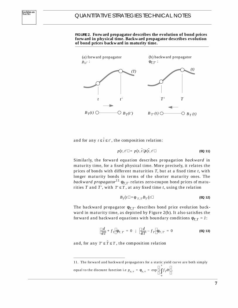
and for any , the composition relation:
(EQ 11)
Similarly, the forward equation describes propagation backward inmaturity time, for a fixed physical time. More precisely, it relates theprices of bonds with different maturities T, but at a fixed time t, withlonger maturity bonds in terms of the shorter maturity ones. Thebackward propagator11 φT,T' relates zero-coupon bond prices of matu-rities T and T', with , at any fixed time t, using the relation
(EQ 12)
The backward propagator φT,T' describes bond price evolution back-ward in maturity time, as depicted by Figure 2(b). It also satisfies theforward and backward equations with boundary conditions φT,T = 1:
; (EQ 13)
and, for any , the composition relation
11. The forward and backward propagators for a static yield curve are both simply
equal to the discount function i.e .
t t t'≤ ≤
p t t',( ) p t t,( )p t t',( )=
pu v, φu v, f τ τdu
v
∫–
exp= =
T' T≤
BT t( ) φT T', BT' t( )=
ddT------- f T+
φT T', 0= ddT'-------- f T'–
φT T', 0=
T' T T≤ ≤
FIGURE 2. Forward propagator describes the evolution of bond pricesforward in physical time. Backward propagator describes evolutionof bond prices backward in maturity time.
BT(t) BT(t')
t t'
(T)
BT' (t) BT (t)
T' T
(t)
(a) forward propagator (b) backward propagatorφT,T' :pt,t' :
7
8
QUANTITATIVE STRATEGIES TECHNICAL NOTESSachsGoldman
The Effective VolatilityTheory
(EQ 14)
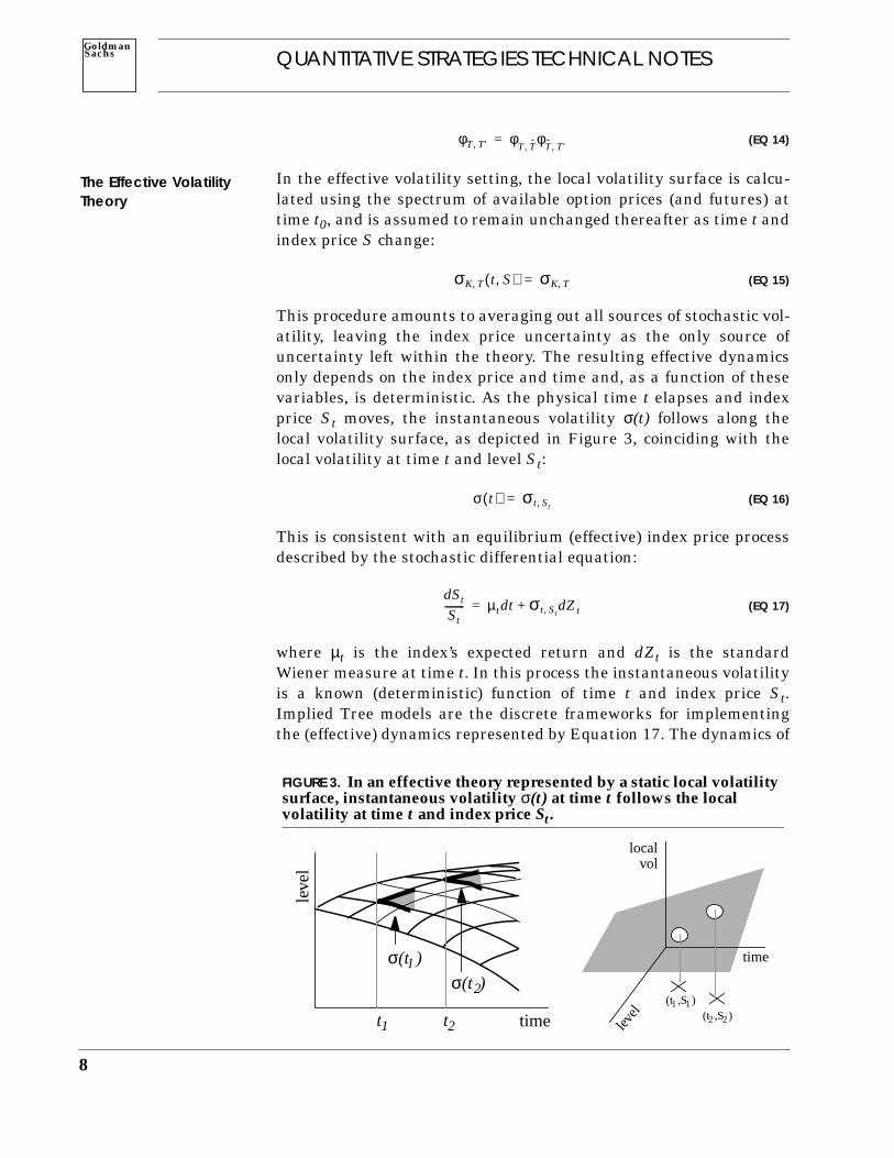
In the effective volatility setting, the local volatility surface is calcu-lated using the spectrum of available option prices (and futures) attime t0, and is assumed to remain unchanged thereafter as time t andindex price S change:
(EQ 15)
This procedure amounts to averaging out all sources of stochastic vol-atility, leaving the index price uncertainty as the only source ofuncertainty left within the theory. The resulting effective dynamicsonly depends on the index price and time and, as a function of thesevariables, is deterministic. As the physical time t elapses and indexprice St moves, the instantaneous volatility σ(t) follows along thelocal volatility surface, as depicted in Figure 3, coinciding with thelocal volatility at time t and level St:
(EQ 16)
This is consistent with an equilibrium (effective) index price processdescribed by the stochastic differential equation:
(EQ 17)
where µt is the index’s expected return and dZt is the standardWiener measure at time t. In this process the instantaneous volatilityis a known (deterministic) function of time t and index price St.Implied Tree models are the discrete frameworks for implementingthe (effective) dynamics represented by Equation 17. The dynamics of
φT T', φT T, φ
T T',=
σK T, t S,( ) σK T,=
FIGURE 3. In an effective theory represented by a static local volatilitysurface, instantaneous volatility σ(t) at time t follows the localvolatility at time t and index price St.
t1
σ(t1)
t2
σ(t2)
time
leve
l
leve
l
time
vollocal
(t1,S1)(t2,S2)
σ t( ) σt St,=
dSt
St-------- µtdt σt St, dZt+=

QUANTITATIVE STRATEGIES TECHNICAL NOTESGoldmanSachs
standard option prices in the effective theory is described by thebackward equation:
(EQ 18)
Since the only remaining source of uncertainty is the index price, thestandard options are completely hedgeable (using index as the hedge)within the effective theory. Equations 16 and 18 then show that theoption price dynamics in this theory is arbitrage-free. Equation 18 isalso the dual of the forward equation satisfied by the standard optionprices:
(EQ 19)
This forward equation is the same as Equation 2 and holds by thedefinition of local volatility, regardless of any specific assumptionsabout the behavior of volatility.
The forward propagator pt,S,t',S' describes the relationship betweenthe option prices at the two points (t, S) and (t', S'), with , for anyK-strike and T-maturity standard option, through the relation
(EQ 20)
The forward propagator pt,S,t',S' describes option price evolution for-ward in time and index price, as illustrated by Figure 4(a). We candefine the forward transition probability density function p(t,S,t',S') interms of the forward propagator as p(t,S,t',S') = er(t'-t) pt,S,t',S'. Itdescribes the total probability that the index price will reach level S'at time t', given that the index price at time t is S. The mathematicalproperties of pt,S,t',S' and p(t,S,t',S') are discussed in Appendix B.
The backward propagator ΦK,T,K',T' describes the relationshipbetween prices of two standard options corresponding to strike-matu-rity pairs (K,T) and (K',T'), with , at a fixed time t and indexprice S, as
(EQ 21)
t∂∂ r δ–( )S
S∂∂ 1
2---σ2
S t, S2S2
2
∂∂ r–+ +
CK T, t S,( ) 0=
T∂∂ r δ–( )K
K∂∂ 1
2---σ2
K T, K2K2
2
∂∂
– δ+ +
CK T, t S,( ) 0=
t t'≤
CK T, t S,( ) pt S t' S', , , CK T, t' S',( ) S'd
0
∞
∫=
T' T≤
CK T, t S,( ) ΦK T K' T', , , CK' T', t S,( ) K'd
0
∞
∫=
9
10
QUANTITATIVE STRATEGIES TECHNICAL NOTESSachsGoldman
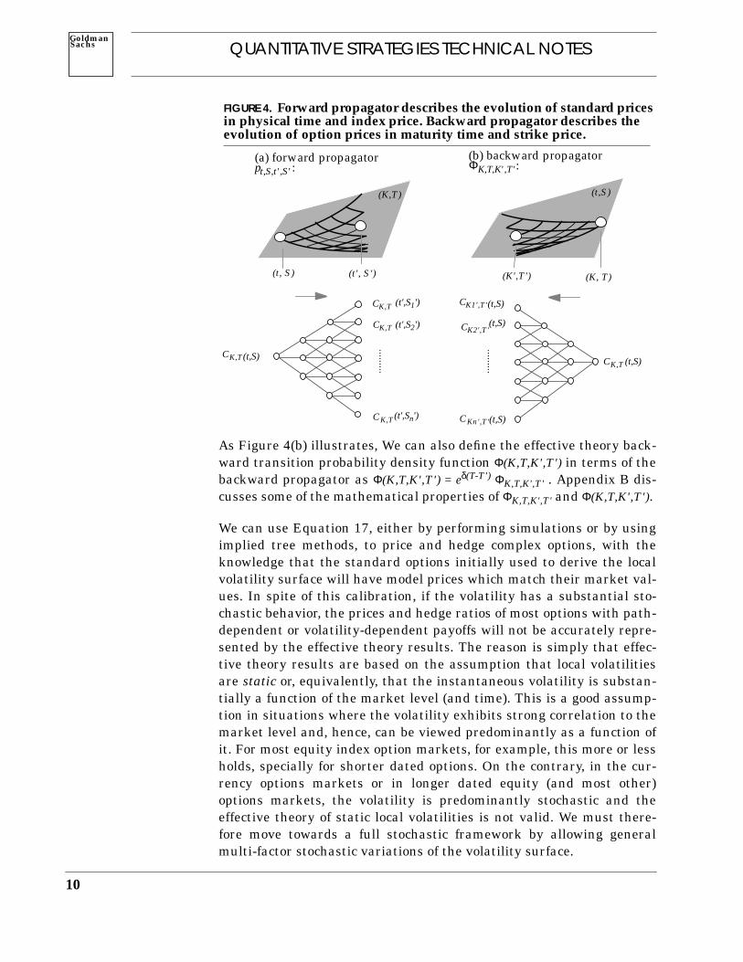
As Figure 4(b) illustrates, We can also define the effective theory back-ward transition probability density function Φ(K,T,K',T') in terms of thebackward propagator as Φ(K,T,K',T') = eδ(T-T') ΦK,T,K',T' . Appendix B dis-cusses some of the mathematical properties of ΦK,T,K',T' and Φ(K,T,K',T').
We can use Equation 17, either by performing simulations or by usingimplied tree methods, to price and hedge complex options, with theknowledge that the standard options initially used to derive the localvolatility surface will have model prices which match their market val-ues. In spite of this calibration, if the volatility has a substantial sto-chastic behavior, the prices and hedge ratios of most options with path-dependent or volatility-dependent payoffs will not be accurately repre-sented by the effective theory results. The reason is simply that effec-tive theory results are based on the assumption that local volatilitiesare static or, equivalently, that the instantaneous volatility is substan-tially a function of the market level (and time). This is a good assump-tion in situations where the volatility exhibits strong correlation to themarket level and, hence, can be viewed predominantly as a function ofit. For most equity index option markets, for example, this more or lessholds, specially for shorter dated options. On the contrary, in the cur-rency options markets or in longer dated equity (and most other)options markets, the volatility is predominantly stochastic and theeffective theory of static local volatilities is not valid. We must there-fore move towards a full stochastic framework by allowing generalmulti-factor stochastic variations of the volatility surface.
FIGURE 4. Forward propagator describes the evolution of standard pricesin physical time and index price. Backward propagator describes theevolution of option prices in maturity time and strike price.
CK,T
CK,T
CK,T
CK,T (t',S1')
(t',S2')
(t',Sn')
(t,S)
......
...
(K,T)
(t, S) (t', S')
(t,S)
(K, T)(K',T')
CK,T
CK1',T'
CK2',T'
CKn',T'
......
...
(t,S)
(t,S)
(t,S)
(t,S)
(a) forward propagator (b) backward propagatorpt,S,t',S': ΦK,T,K',T':

QUANTITATIVE STRATEGIES TECHNICAL NOTESGoldmanSachs
TOWARDS A STOCHASTICTHEORY OF VOLATILITY
The Stochastic InterestRate Theory
To allow for stochastic dynamics we must introduce exogenous sto-chastic structure on the effective theory. In general, there are fewrestrictions on the choice of this structure. One important restriction,which is the cornerstone of the arbitrage framework, is the absence ofany explicit future arbitrage opportunities in the final stochastic the-ory. Another restriction is how close the number or the behavior ofthe stochastic factors are to what is empirically observed. For now, wewill consider very general (but sufficiently regular) stochastic struc-tures and discuss the conditions which must be imposed upon themto guarantee the absence of arbitrage. Let us briefly examine the sto-chastic interest rate theory first.
Figure 5 illustrates the dynamics of the forward rates in the stochas-tic framework. Here, the forward rate curve is allowed to fluctuatestochastically with several independent stochastic factors repre-sented by Brownian motions Wi, i = 1, ...,n, with factor volatilities
generally depending on both maturity T and time t, accordingto the stochastic differential equation:
(EQ 22)
In the family of processes described by Equation 22, the volatilitycoefficients reflect the sensitivities of specific maturity forwardrates to the random shocks introduced by the Brownian motions Wi.These coefficients are left unrestricted, except for mild measurabilityand integrability conditions, and can depend on the past histories of
0 t1
r(t1)
rate
r(t 0)
time
FIGURE 5. In a stochastic interest rate theory spot rate r(t) follows theinstantaneous forward rate ft(t).
fT(t0)
fT(t1)
ϑiT t( )
d f T t( ) αT t( )dt ϑTi
t( )dWti
i 1=
n
∑+=
ϑiT t( )
11

12
QUANTITATIVE STRATEGIES TECHNICAL NOTESSachsGoldman
The Stochastic VolatilityTheory
the Brownian motions Wi. The drift coefficients must also sat-isfy mild measurability and integrability conditions, but must be fur-ther constrained by the no-arbitrage requirement.
The spot rate at time t, r(t), is the instantaneous forward rate at timet, i.e, . The stochastic integral equation satisfied by thespot rate is found by integrating Equation 22 and evaluating theresult at T = t. It is given by
(EQ 23)
It has been argued by Heath, Jarrow and Morton, that there will beno explicit arbitrage opportunities in the theory defined by Equation23 if (and only if) the drift coefficients are of the form:
(EQ 24)
Here , i = 1, ..., n, denote the market prices of risk, which can notexplicitly depend on maturity T but are otherwise arbitrary. Underthese conditions, they have shown that markets are complete andcontingent claims prices are independent of the market prices of risk.
Our goal is to introduce a similar stochastic structure on the localvolatility surface. To do so, we allow the surface to undergo stochasticfluctuations with several independent stochastic factors, W0, W1,...,Wn, based on the following stochastic differential equation12:
(EQ 25)
We include W0 = Z, the index price’s source of uncertainty, among thefactors so that the stochastic variations of the local volatility surfacemay depend on the prevailing market level. The family of processesof Equation 25 defines a multi-factor dynamics for the local volatilitysurface, as illustrated by Figure 6. These processes can be integrated,
12. The variable S in the expression for local volatility σΚ,Τ(t, S) is included for nota-tional purposes and does not imply dependence solely on the spot index level. In fact,local volatilities generally depend on the entire history of the index price and otherstochastic factors. Aside from time t and index price S, all other variables have beenexplicitly omitted from expressions for local volatilities, drifts and factor volatilities.
αT t( )
r t( ) f t t( )=
r t( ) f t 0( ) αt u( ) ud0
t
∫ ϑit u( ) Wi
ud0
t
∫i 1=
n
∑+ +=
αT t( ) ϑTi t( ) ϑu
i t( ) udt
T
∫ λi t( )+
i 1=
n
∑=
λi t( )
dσ2K T, t S,( ) αK T, t S,( )dt θi
K T, t S,( )dWit
i 0=
n
∑+=

QUANTITATIVE STRATEGIES TECHNICAL NOTESGoldmanSachs
starting from a fixed (non-random) initial local volatility surfaceσK,T(0,S0) at time t = 0, as
(EQ 26)
The factor volatility reflects the sensitivity of local volatilitiesσK,T(t,S), across the whole surface, to the shock introduced by theBrownian motion Wi. Except for mild measurability and integrabilityconditions13, the family of factor volatilities are unrestricted, generallydepending on time and index price, and on the factors or their past histo-ries. However, for the sake of brevity we have omitted explicit referencesto all variables other than time t and index price S from the expressionsfor factor volatilities, and we will do the same for other quantities suchas drift coefficients and local volatilities.
The spot volatility (or instantaneous volatility) at time t, σ(t), is theinstantaneous local volatility at time t and level St, i.e
(EQ 27)
It describes the variability of index price return process, as given by thedifferential equation
13. The factor volatility functions are assumed to be positive, adapted andjointly measurable with respect to the Borel σ-algebra restricted to , forsome fixed maximum time T*. They must also satisfy , i = 0, ...,n, toassure regularity of spot volatility process, and certain additional integrability conditionsto assure regularity of the standard option price processes.
FIGURE 6. In a stochastic volatility theory instantaneous volatility σ(t)follows the local volatility σSt,t (t,St), at time t and index price St.
0 t1 time
σ(t1)σ(t0)
leve
l
level
time
localvol
(t1,S1)(t2,S2)
σ2K T, t St,( ) σ2
K T, 0 S0,( ) αK T, u Su,( ) ud0
t
∫ θiK T, u Su,( ) Wi
ud0
t
∫i 0=
n
∑+ +=
θiK T, t S,( )
θiK T, t S,( )
0 t T T∗≤ ≤ ≤θi
K T,( )2 u Su,( ) ud0
T
∫ ∞<
σ t( ) σSt t, t St,( )=
13

14
QUANTITATIVE STRATEGIES TECHNICAL NOTESSachsGoldman
The HJM Conditions and theStochastic Theory of InterestRates
(EQ 28)
or its integral form
(EQ 29)
where µt is the index’s expected return. Setting T = t and K = St inEquation 26 we find the stochastic integral equation satisfied by thespot volatility as
(EQ 30)
The drift coefficients must also satisfy mild measurabilityand integrability conditions, but they must be further restricted bythe requirement that the stochastic theory described by Equations 28and 30 disallows explicit arbitrage opportunities among the standardoptions, forwards and their underlying index. This is similar to theHJM arbitrage conditions on the spot rate process. Let us brieflyexamine (a variation of) the HJM argument below.
The bond price dynamics corresponding to the forward rate process ofEquation 85 is, by applying Ito’s lemma, described by the stochasticintegral equation
(EQ 31)
The symbol here denotes the variational (or functional) derivativewith respect to the function f evaluated at u. The first term in thisequation describes precisely the effective theory bond price dynamicsrestricted to the fixed forward rate curve fT(t) at time t. The next twoterms describe the bond price dynamics resulting from the stochasticvariations of the effective theory (defined by fT(t)) during the nextinfinitesimal time interval dt.
It follows from the definition of the forward rates (Equation 1) thatthe price of a T-maturity zero-coupon bond with unit face, at time t, isgiven by
dSt
St-------- µtdt σ t( )dWt
0+=
St S0 µuSu ud0
t
∫ σ u( )Su Wu0d
0
t
∫+ +=
σ2 t( ) σ2t St, 0 S0,( ) αt St, u Su,( ) ud
0
t
∫ θit St, u Su,( ) Wi
ud0
t
∫i 0=
n
∑+ +=
αK T, t S,( )
dBT t( ) r t( )BT t( )dtδBT t( )δ f u t( )----------------- f u t( )d u +d
t
T
∫+=
12---
δ2BT t( )δ f u t( )δ f u' t( )---------------------------------- f u t( )d f u' t( )d ud u'd
t
T
∫t
T
∫δ
δ f u----------

QUANTITATIVE STRATEGIES TECHNICAL NOTESGoldmanSachs
(EQ 32)
From this expression it is simple to see that for any u ( ):
(EQ 33)
Another way of seeing this is by noticing how the forward and back-ward propagators, pt,t' and φT,T', corresponding to an otherwise fixed(non-random) forward rate curve, respond to sudden changes of aspecific forward rate fu along the curve. It is simple to see that pt,t'satisfies the following relation, as depicted in Figure 7(a):
(EQ 34)
and, as shown in Figure 7(b), that φT,T' satisfies the relation:
(EQ 35)
These relations combined, respectively, with Equations 9 and 12,again lead to Equation 33.
Similarly, we can show that for the second order varia-tional derivatives are given by:
BT t( ) f u t( ) udt
T
∫– exp=
t u T≤ ≤
δBT t( )δ f u t( )----------------- B– T t( )=
FIGURE 7. Sensitivity of the forward and backward propagators pt,t'and φT,T' to the sudden changes of the forward rate fu.
(a) forward propagator (b) backward propagator
t t'u
-1
t t'u u+du T' Tu u+du
T' Tu
-1
δp t t',( )δ f u
------------------- p– t u,( )p u t',( ) p t t',( )–= =
δφT T',
δ f u-------------- φ– T u, φu T', φT T',–= =
t u u' T≤ ≤ ≤
15

16
QUANTITATIVE STRATEGIES TECHNICAL NOTESSachsGoldman
THE NO-ARBITRAGE CONDITIONSAND THE STOCHASTIC THEORY OFVOLATILITY
(EQ 36)
The special fu-independent form of variational relations 33-36 canbe directly attributed to the special form of the functional relation-ship between the zero-coupon bond prices and the forward rates asdescribed by Equation 32. This feature underlies the special sim-plicity of no-arbitrage conditions in the HJM framework.
Using Equations 22, 33 and 36 inside Equation 31 we find
(EQ 37)
If the drift coefficients satisfy the no-arbitrage conditions ofEquation 24 for some set of market prices of risk , then Equa-tion 37 shows that in terms of the equivalent measure
, defined by the Brownian motions, i = 1, ..., n, the dynamics of zero-coupon bond
prices is:
(EQ 38)
Therefore, {dWi ; i = 1,...,n} defines an equivalent martingale mea-sure under which the rescaled bond prices for allmaturities T are jointly martingale. Under this measure the inter-est rate contingent claims prices are independent of the marketprices of risk and, hence, remain preference-free.
The standard option prices CK,T(t,S) are functionals of the local vol-atilities at time t and market level S, just as bond prices BT(t) arefunctionals of the forward rates at time t. As a result, the dynami-cal variations of the local volatility surface induce correpsondingdynamical variations of the standard option prices. During a timeinterval dt, the index price moves and the local volatilities alsochange. We can think of the local volatility changes as comprised oftwo components. A predictable component, due to movements oftime and index price restricted to the static local volatility surfaceσK,T(t,S) at time t and level S, and a non-predictable (stochastic)component due to dynamic fluctuations away from this surface. It is
δ2BT t( )δ f u t( )δ f u' t( )---------------------------------- BT t( )=
dBT t( )BT t( )----------------- r t( )dt ϑu
i t( ) udt
T
∫
i 0=
n
∑ dWti– –=
αu t( ) ϑui t( ) ϑv
i t( ) vdt
u
∫i 1=
n
∑– udt
T
∫
dt
αT t( )λi t( )
dWi dWi λidt+=
Wit Wi
t λi u( ) ud0
t
∫+=
dBT t( )BT t( )----------------- r t( )dt ϑu
i t( ) udt
T
∫
i 1=
n
∑ dWti
–=
BT t( ) r u( ) ud0
t
∫–
exp

QUANTITATIVE STRATEGIES TECHNICAL NOTESGoldmanSachs
somewhat simpler, but entirely equivalent, to work with the transi-tion probabilities, instead of option prices. The transition probability,PK,T(t,S), describes the total probability that the index price willreach level K at time T, given that the index price at time t is S, whenboth the index price and volatility are stochastic. It is related to theoption prices CK,T(t,S) through a general and well-known14 formula:
(EQ 39)
The dynamical evolution of transition probabilities PK,T(t,S) based onthe local volatility process of Equation 26 is given by the stochasticintegral equation:
(EQ 40)
All the probability and local volatility expressions in this equationare evaluated at (t,S). The first term describes the effective dynamicsof the transition probabilities PK,T(t,S) restricted to the fixed localvolatility surface σK,T(t,S), prevailing at time t and level S. Thebracket symbol, , therefore, expresses the fact that in thisterm the future volatility is a deterministic function of the futuretime T and market level K, given by σK,T(t,S) viewed as function ofthese two variables. The next two terms describe the dynamical vari-ations of the transition probabilities resulting from the stochasticfluctuations of the local volatility surface during the next instant oftime dt.
Contrary to Equation 32, in general there are no explicit expressionsdescribing the functional relationship between option prices and localvolatilities. Therefore, we can not directly compute the variational
14. See Breeden and Litzenberger [1978].
PK T, t S,( ) er T t–( )K2
2
∂∂ CK T, t S,( )=
dPK T, t∂∂PK T, µ t( )S
S∂∂PK T, 1
2---σ2 t( )S2
S2
2
∂∂ PK T,+ +
dt σ t( )SS∂
∂PK T, dW0 t( )+t S,( )
= +
δPK T,
δσ2K' T',
------------------ σ2K' T',d K'd T'd
0
∞
∫t
T
∫ +
12---
δ2PK T,
δσ2K' T', δσ2
K'' T'',---------------------------------------- σ2
K' T',d σ2K'' T'',d K'd K''d T' T''dd
0
∞
∫0
∞
∫t
T
∫t
T
∫
…[ ] t S,( )
17

18
QUANTITATIVE STRATEGIES TECHNICAL NOTESSachsGoldman
derivatives in Equation 40. Instead, we can look at the variations ofthe forward and backward transition probabilities with respect to thespecific local volatilities. As shown in Appendix C and illustrated inFigure 8, the forward transition probability p(t,S,t',S'), associatedwith the non-random local volatility surface σK,T(t,S) prevailing attime t and spot price S, has the following variational derivative withrespect to the local volatility σv,u(t,S) on the surface, corresponding tofuture maturity u and market level v:
(EQ 41)
FIGURE 8. Sensitivity of the forward and backward transitionprobabilities p(t,S,t',S') and Φ(K,T,K',T') to the sudden changes of thelocal volatility σv,u.
u v,( ) t' S',( )t S,( )
t S,( )t' S',( )
t S,( ) t' S',( )
u v,( )
v2
v2
2
∂∂
–
K T,( )K ' T',( )
K T,( )K ' T',( )
v u,( )
v2
v2
2
∂∂
–
K ' T',( ) K T,( )v u,( )
(a) forward (b) backward
δp t S t' S', , ,( )δσ2
v u,---------------------------------
12---p t S u v, , ,( )v2
v2
2
∂∂ p u v t' S', , ,( )=

QUANTITATIVE STRATEGIES TECHNICAL NOTESGoldmanSachs
This relation holds for any u in the range , otherwise the vari-ational derivative is equal to zero. Similarly, the backward transitionprobability Φ(K,T,K',T') satisfies, for , the relation
(EQ 42)
and zero otherwise. Using Equations 21 and 39, the standard optionprices CK,T(t,S) and transition probabilities PK,T(t,S) satisfy similarrelationships for :
(EQ 43)
and
(EQ 44)
in which the effective transition probabilities and corre-spond to the static local volatility surface σK,T(t,S) prevailing at timet and market level S. In arriving at Equations 43 and 44 we have alsoused the following identities:
(EQ 45)
(EQ 46)
(EQ 47)
As discussed in Appendix B, these identities are all consequences ofthe fact that the effective theory associated with σK,T(t,S) embodiesall the information necessary for pricing standard options of allstrikes and maturities correctly.
Taking the variational derivatives of both sides of Equations 41 and42 with respect to the local volatility σv',u' we find the second ordervariational derivatives as
(EQ 48)
t u t'≤ ≤
T' u T≤ ≤
δΦ K T K' T', , ,( )δσ2
v u,----------------------------------------
12---Φ K T v u, , ,( )v2
v2
2
∂∂ Φ v u K' T', , ,( )=
t u T≤ ≤
δCK T, t S,( )δσ2
v u,----------------------------
12---Φ K T v u, , ,( )v2
v2
2
∂∂ Cv u, t S,( )=
δPK T, t S,( )δσ2
v u,----------------------------
12---p t S u v, , ,( )v2
v2
2
∂∂ p u v T K, , ,( )=
p …( ) Φ …( )
PK T, t S,( ) p t S T K, , ,( )=
p t S T K, , ,( ) er T t–( )
K2
2
∂∂ CK T, t S,( )=
Φ K T S t, , ,( ) eδ T t–( )
S2
2
∂∂ CK T, t S,( )=
δp t S t' S', , ,( )δσ2
v u, δσ2v' u',
----------------------------------14---p t S u v, , ,( )v2
v2
2
∂∂ p u v u' v', , ,( )v'
2
v'2
2
∂∂ p u' v' t' S', , ,( )=
19
20
QUANTITATIVE STRATEGIES TECHNICAL NOTESSachsGoldman
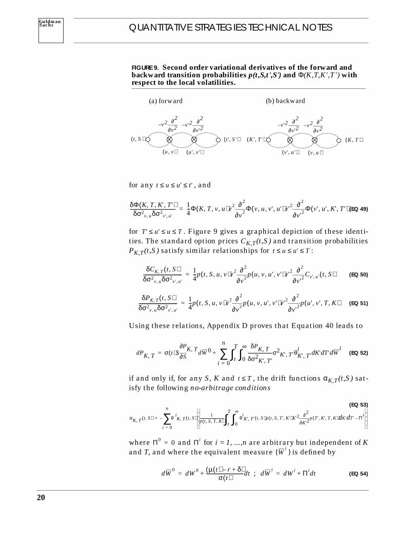
for any , and
(EQ 49)
for . Figure 9 gives a graphical depiction of these identi-ties. The standard option prices CK,T(t,S) and transition probabilitiesPK,T(t,S) satisfy similar relationships for :
(EQ 50)
(EQ 51)
Using these relations, Appendix D proves that Equation 40 leads to
(EQ 52)
if and only if, for any S, K and , the drift functions αK,T(t,S) sat-isfy the following no-arbitrage conditions
(EQ 53)
where and for i = 1, ...,n are arbitrary but independent of Kand T, and where the equivalent measure { } is defined by
; (EQ 54)
t u u' t'≤ ≤ ≤
δΦ K T K' T', , ,( )δσ2
v u, δσ2v' u',
----------------------------------------14---Φ K T v u, , ,( )v2
v2
2
∂∂ Φ v u v' u', , ,( )v'
2
v'2
2
∂∂ Φ v' u' K' T', , ,( )=
T' u' u T≤ ≤ ≤
FIGURE 9. Second order variational derivatives of the forward andbackward transition probabilities p(t,S,t',S') and Φ(K,T,K',T') withrespect to the local volatilities.
K ' T',( )
v' u',( )
v'2v'2
2
∂∂
–
v u,( )
v2v2
2
∂∂
–
K T,( )t S,( )
u v,( )
v2v2
2
∂∂
–
u' v',( )
v'2v'2
2
∂∂
–
t' S',( )
(a) forward (b) backward
t u u' T≤ ≤ ≤
δCK T, t S,( )δσ2
v u, δσ2v' u',
----------------------------------14---p t S u v, , ,( )v2
v2
2
∂∂ p u v u' v', , ,( )v'
2
v'2
2
∂∂ Cv' u', t S,( )=
δPK T, t S,( )δσ2
v u, δσ2v' u',
----------------------------------14---p t S u v, , ,( )v2
v2
2
∂∂ p u v u' v', , ,( )v'
2
v'2
2
∂∂ p u' v' T K, , ,( )=
dPK T, σ t( )SS∂
∂PK T, dW0δPK T,
δσ2K' T',
-----------------------σ2K' T', θK' T',
iK'd T'd W
id
0
∞∫t
T
∫i 0=
n
∑+=
t T≤
αK T, t S,( ) θiK T, t S,( ) 1
p t S T K, , ,( )------------------------------ θiK' T', t S,( )p t S T' K', , ,( )K'2
K'2
2
∂∂ p T' K, ' T K, ,( ) K'd T'd
0
∞
∫t
T
∫ Πi–
i 0=
n
∑–=
Π0 0= Πi
Wi
dW0
dW0 µ t( ) r– δ+( )σ t( )---------------------------------dt+= dW
idWi Πidt+=

QUANTITATIVE STRATEGIES TECHNICAL NOTESGoldmanSachs
StOCHASTIC IMPLIED TREES
The quantities denote the market prices of risk associated with thevolatility risk factors Wi, i = 1, ..., n, while µ - (r-δ) is the market priceof risk associated with the index price risk factor W0. Equation 52shows that under the no-arbitrage conditions the measure { ; i =1, ...,n} is an equivalent martingale measure, with respect to whichthe rescaled index price and rescaled option prices for all strikes andmaturities are simultaneously martingales.
These no-arbitrage conditions in the present case are significantlymore involved than the HJM no-arbitrage conditions described in theprevious section. The basic reason is that local volatilities span a(two-dimensional) surface on which (forward and backward) propaga-tion depends, in a rather complicated and non-linear manner, on thestructure of local volatilities across the whole surface. This is evidentby the apparent complexity of Equations 44 and 51 as compared tothe simplicity of the corresponding Equations 33 and 36 in the inter-est rate framework. It is, therefore, rather difficult to use the no-arbi-trage conditions for stochastic volatility in their continuous formdirectly.
In the next section we introduce Stochastic Implied Trees as a dis-crete-time framework for describing arbitrage-free stochastic varia-tions of the local volatility surface.
Figure 11 gives a schematic illustration of the dynamics in a stochas-tic volatility theory. As the physical time moves forward, the indexprice changes and, simultaneously, all local volatilities on the volatil-ity surface undergo multi-factor stochastic variations.
Πi
dWi
FIGURE 11. Schematic illustration of the dynamics of the index priceand local volatility surface in a stochastic volatility theory.
time
21

22
QUANTITATIVE STRATEGIES TECHNICAL NOTESSachsGoldman
To provide a more quantitative description of this stochasticdynamics we choose to work within a discrete-time frameworkdescribed by a Stochastic Implied Tree. These trees are extensionsof the standard (non-stochastic) implied trees, which are used todescribe effective volatility models (see Derman, Kani and Chriss[1996]). Figure 12 shows an example of a 1-year, 5-period standardimplied trinomial tree which is calibrated to a market where at-the-money implied volatility is 25% and there is an implied volatilityskew of 0.5% point per 10 strike points. In an implied trinomial tree
FIGURE 12. Example of an Implied Trinomial Tree describing aneffective volatility theory.
100.00
83.80
119.34 119.34 119.34 119.34
100.00 100.00 100.00 100.00
142.41 142.41 142.41
70.22 70.22 70.22
169.95 169.95
58.84 58.84
49.31
202.81
83.8083.8083.80
state space:
0.249
0.240 0.236 0.235
0.249 0.247 0.247
0.224 0.221
0.313 0.298
0.188
0.327
0.2640.2690.272
local volatilities:
0.259
0.241 0.236 0.233
0.259 0.255 0.255
0.214 0.209
0.392 0.358
0.160
0.425
0.2870.2960.304
0.241
0.220 0.213 0.209
0.241 0.236 0.236
0.188 0.181
0.400 0.359
0.123
0.438
0.2740.2850.294
probabilities: probabilities:forward diffusion downforward diffusion up
0.000
1.000 0.285 0.2780.000 0.306 0.301
1.000 0.253
0.000 0.000
1.000
0.000
0.3500.0000.000
0.189
0.246
0.2750.301
0.339
0.423
0.000
0.000
1.000
0.000
0.000 0.000 0.1760.000 0.200 0.195
0.000 0.000
1.000 0.331
0.000
1.000
0.2360.2441.000
0.000
0.150
0.1740.195
0.227
0.298
0.363
1.000
0.000probabilities: probabilities:
backward diffusion up backward diffusion down

QUANTITATIVE STRATEGIES TECHNICAL NOTESGoldmanSachs
the location of the nodes, or the state space, is more or less arbitrarily.Once the state space is fixed, however, the transition probabilities atdifferent nodes are determined from the requirement that standardoptions and forwards with strike prices coinciding with those nodesand maturing at different periods of the tree all have prices using thetree which match their market prices. Since local volatility at anynode depends on the nodal levels and the transition probabilities tothe nearby nodes, the local volatilities at different nodes are alsodetermined in this way.
Stochastic implied trinomial trees are extensions of the implied trino-mial tree in which the transition probabilities are, in addition,allowed to vary stochastically, with several stochastic factors, as timeelapses and index level moves. The index level is allowed to moverandomly from node to node, while the local volatilities, and simulta-neously the transition probabilities corresponding to the futurenodes, all vary stochastically across the tree. This behavior is shownin Figure 13.
Starting from any initial node, the possible future movements of thelocal volatility surface must be restricted to guarantee absence of anyarbitrage opportunities in the discrete theory represented by the sto-chastic implied tree. As discussed earlier, this is equivalent to therequirement that the total transition probabilties to all future nodesbe simultaneously martingales on the tree. This is also the same as
FIGURE 13. In a Stochastic Implied Tree, as the index moves from nodeA to node B in a single time step, the local volatilities and transitionprobabilities, for every node on the future subtree beginning at nodeB, vary stochastically with multiple stochastic factors.
A
B
23

24
QUANTITATIVE STRATEGIES TECHNICAL NOTESSachsGoldman
Our Notation in Discrete Time
the requirement that all rescaled standard option prices be simulta-neously martingales on the tree. As Figure 14 shows, during the timeinterval ∆t, the spot price will move randomly (by amount ∆S) to oneof the nearby nodes and, at the same time, the local volatility surfacewill assume one of its N possible configurations, w1, ...,wN. As aresult, the total transition probability PK,T(t,S) to any given futurenode (K,T) also moves to one of its several possible values P(i)
K,T(t+∆t,S+∆S), i = 1, ..., M, during this time interval. To guarantee no-arbi-trage, PK,T must be a martingale (fair game), that is it must equalthe expectation , under some (equivalent) measure, of its future val-ues P(i)
K,T for all the future nodes (K,T) on the tree.
To make positivity manifest, it is more convenient to redefine thedrift and volatility functions in Equation 25 as and
, l = 0, ..., n, and begin by discretizing the followingcontinuous-time differential equation:
(EQ 55)
We let the integer pair (i,j) label the node (ti,Sj) describing the cur-rent location (i.e (t,S)) of the index at the ith step of the simulation.
t t +∆t
P K,T
P (1)K,T
P (M)K,T
FIGURE 14. During a time step ∆t, the total transition probability PK,Twill move to one of M values P(i)
K,T , i = 1, ...,M, as index price movesrandomly to one of the nearby nodes and the local volatility surfaceassumes one of N possible configurations.
t t +∆t
w
w 1
w N
αK T, αK T, σK T,2→
θlK T, θl
K T, σK T,2→
dσ2K T, t S,( )
σ2K T, t S,( )
------------------------------- αK T, t S,( )dt θlK T, t S,( )dWt
l
l 0=
n
∑+=

QUANTITATIVE STRATEGIES TECHNICAL NOTESGoldmanSachs
We also let the pair (n,m) label the future node (tn,Sm) correspondingthe future time and level (i.e (T,K)). Then the discrete form of Equa-tion 55 can be written as
(EQ 56)
The vector (∆Wi0, ∆Wi
1, ..., ∆Win) is random and is drawn, at time i,
from the sample space of the increments of n independent Brownianmotions Wl.
The volatility parameters are pre-specified but the driftparameters must be determined from the no-arbitragerequirements that the total probabilities of arriving at thefuture node (n,m) from the (fixed) initial node (i,j) must be jointlymartingales for all future nodes (n,m). As we shall argue below, thesemartingale conditions are precisely enough to completely determineall the drift parameters step by step during the simulation process.
A Stochastic Implied Tree simulation begins with the construction ofa trinomial implied tree calibrated to today’s prices of standardoptions and forwards. The simulation begins at the node (0,0) of thistree. During the first simulation step the drift parameters ,for all future nodes (m,n), are determined from the martingale condi-tions on the total probabilities . Figure 15 illustrates that
∆σ2m n, i j,( ) σ2
m n, i j,( ) αm n, i j,( )∆ti θm n,l i j,( )∆Wi
l
l 0=
n
∑+=
θm n,l i j,( )
αm n, i j,( )Pm n, i j,( )
αm n, 0 0,( )
Pm n, 0 0,( )
FIGURE 15. The drift parameter α0,0(0,0) in a Stochastic Implied Tree isdetermined from the martingale condition on the total transitionprobability P1,2(0,0).
(0,0)
(1,2)
(0,0)
(1,2)
(0,0)
(1,2)
a0,0(0,0)
P1,2 (0,0) is martingale
25

26
QUANTITATIVE STRATEGIES TECHNICAL NOTESSachsGoldman
the drift parameter is determined from the martingale con-dition for This also guarantees that the transition probabili-ties and are martingales. The reason is that theseprobabilities are constrained by two extra conditions which musthold irrespective of the specific behavior of the local volatilities:
(EQ 57)
The first condition is the normalization condition, requiring that thesum of the three total transition probabilities at time t1 must beunity. The second is the forward condition, requiring that the t1-maturity forward price at time t0 must match its risk-neutral value.
In a similar way, the three drift parameters , andare determined from the martingale conditions of the three
total transition probabilities , and . Theremaining transition probabilities and will thenalso be martingales due to the normalization and forward conditionsat time t2. In this way all drift parameters will be deter-mined during the first simulation step. Finally, to complete this stepwe draw a random vector (∆W0
0, ∆W01, ..., ∆W0
n) from the samplespace of the increments of Wi at time t0, and use this vector to simul-taneously arrive at a (random) new location for the index price andnew values for all future local volatilities. Equation 56 is useddirectly with i = j = 0 to calculate the new local volatility values fromthis choice of the random vector. As for the index price, we use therandom number ∆W0
0 to determine which of the three possible futurenodes (i.e (1,2), (1,1) or (1,0)) does the index price moves to duringtime interval ∆t. Figure 16 gives one simple possible method for
α0 0, 0 0,( )P1 2, 0 0,( )
P1 1, 0 0,( ) P1 0, 0 0,( )
P1 0, 0 0,( ) P1 1, 0 0,( ) P1 2, 0 0,( )+ + 1=
P1 0, 0 0,( )S1 0, P1 1, 0 0,( )S1 1, P1 2, 0 0,( )S1 2,+ + S0 0, er δ–( ) t1 t0–( )
=
α1 2, 0 0,( ) α1 1, 0 0,( )α1 0, 0 0,( )
P2 4, 0 0,( ) P2 3, 0 0,( ) P2 2, 0 0,( )P2 1, 0 0,( ) P2 0, 0 0,( )
αm n, 0 0,( )
FIGURE 16. Determining which node the index price will go to duringone simulation step using the renormalized random number ∆Wi
0.
(i, j)
(i+1, j+2) if ∆Wi0 >= Pm + Pd
(i+1, j+1) if ∆Wi0>= Pd and∆Wi
0 < Pm + Pd
(i+1, j) if ∆Wi0 < Pd
Pu = Pu(i,j)
Pd = Pd(i,j)
Pm = Pm(i,j)

QUANTITATIVE STRATEGIES TECHNICAL NOTESGoldmanSachs
A SIMPLE EXAMPLE
doing this starting from an arbitrary initial node (i,j). First ∆Wi0 is
renormalized to represent a uniformly-distributed random numberbetween 0 and 1. Let Pu(i,j), Pm(i,j) and Pd(i,j) denote the one periodtransition probabilities, prevailing at time ti and index price Sj, fromthe node (i,j) to the up, middle and down nodes at time ti+1. We thencompare our random number with these three probabilities. If it issmaller than Pd(i,j), we move the index price to the down node. Onthe other hand, if the random number is greater than the sum Pu(i,j)+ Pm(i,j), we allow the index price to move to the up node. In everyother case we move the index price to the middle node at the nexttime period.
We can continue this procedure, step-by-step, for any point (i,j) alonga simulated path through the stochastic implied tree. First, all thedrift parameters are determined from the martingale condi-tions on . Appendix E gives the necessary details for doingthis calculation. Subsequently, these drift parameters are used togenerate arbitrage-free (random) movements of the future local vola-tility surface as the index price moves randomly forward across thetree. We can generate many such sample paths through the tree.Along each path, the movements of the index price and the local vola-tility surface are random realizations of an arbitrage-free dynamics,which step-by-step guarantees absence of arbitrage opportunitiesamong different standard option (and forward) contracts and theirunderlying index within the discrete time framework of the stochas-tic implied tree.
Consider a one-factor stochastic volatility model with a lognormalvolatility of volatility structure, as described by the following pair ofstochastic differential equations:
where . For the purpose of this example we take thevolatility coefficient to be constant, so that the factor W1 has theinterpretation of a simultaneous constant (proportional) shift in alllocal volatilities. All the other quantities can depend on t, S, factorsW0 and W1 or their past values. More specifically, we consider a 1-year, 5-period example with the initial term and strike structure of
αm n, i j,( )Pm n, i j,( )
dSS
------ µdt σdW0+=
dσ2K T,
σ2K T,
----------------- αK T, dt θdW1+=
σ t( ) σt St, t St,( )=
θ
27
28
QUANTITATIVE STRATEGIES TECHNICAL NOTESSachsGoldman
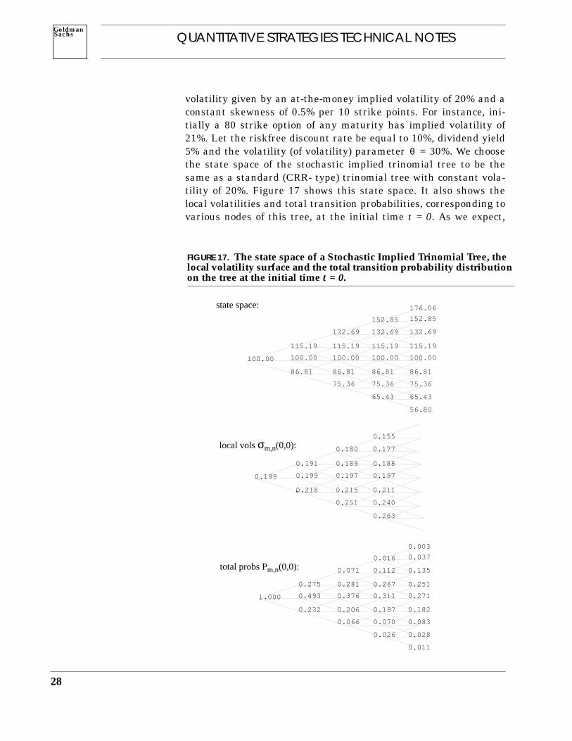
volatility given by an at-the-money implied volatility of 20% and aconstant skewness of 0.5% per 10 strike points. For instance, ini-tially a 80 strike option of any maturity has implied volatility of21%. Let the riskfree discount rate be equal to 10%, dividend yield5% and the volatility (of volatility) parameter = 30%. We choosethe state space of the stochastic implied trinomial tree to be thesame as a standard (CRR- type) trinomial tree with constant vola-tility of 20%. Figure 17 shows this state space. It also shows thelocal volatilities and total transition probabilities, corresponding tovarious nodes of this tree, at the initial time t = 0. As we expect,
θ
FIGURE 17. The state space of a Stochastic Implied Trinomial Tree, thelocal volatility surface and the total transition probability distributionon the tree at the initial time t = 0.
100.00
86.81
115.19 115.19 115.19 115.19
100.00 100.00 100.00 100.00
132.69 132.69 132.69
75.36 75.36 75.36
152.85 152.85
65.43 65.43
56.80
176.06
86.8186.8186.81
state space:
0.199
0.191 0.189 0.188
0.199 0.197 0.197
0.180 0.177
0.251 0.240
0.155
0.263
0.2110.2150.218.
local volsσm,n(0,0):
1.000
0.182
0.275 0.281 0.267 0.251
0.493 0.376 0.311 0.271
0.071 0.112 0.135
0.066 0.070 0.083
0.016 0.037
0.026 0.028
0.011
0.003
0.1970.2060.232
total probs Pm,n(0,0):

QUANTITATIVE STRATEGIES TECHNICAL NOTESGoldmanSachs
local volatilities increase as the index level decreases roughly twiceas fast as implied volatilities. Also the probability distribution isskewed (around the forward price) towards the lower index levels.The first step toward the construction of the stochastic implied tree isto determine the drift coefficients at time t0 = 0. Appendix Egives the formulas for directly calculating these coefficients, which
αm n, 0 0,( )
FIGURE 18. The first step of the Stochastic Implied Tree constructionconsists of determining all the drift coefficients αm,n(0,0), at time t0 =0, from the martingale conditions for the total probabilities Pm,n(0,0).
1.0000.182
0.275 0.281 0.267 0.2510.493 0.376 0.311 0.271
0.071 0.112 0.135
0.066 0.070 0.083
0.016 0.037
0.026 0.0280.011
0.003
0.1970.2060.232
total probs Pm,n(0,0):
-0.044-0.184 -0.037 0.0090.139 0.072 0.063
-0.298 -0.194
-0.369 -0.195
-0.381
-0.452
-0.043-0.051-0.232
drifts αm,n(0,0):
choose a random vector (∆W0, ∆W1) -> (up, up)
0.1990.191 0.189 0.1880.199 0.197 0.197
0.180 0.177
0.251 0.240
0.155
0.263
0.2110.2150.218.
local volsσm,n(0,0):
step 1
29

30
QUANTITATIVE STRATEGIES TECHNICAL NOTESSachsGoldman
are shown in Figure 18. We can justify the numbers by examiningwhat can happen to the total transition probabilities during the nexttime interval ∆t. All local volatilities will simultaneously move, withprobability of 1/2, to their up values, , or their down val-ues, , as given by
1.0000.175
0.343 0.278 0.243 0.2200.346 0.303 0.256 0.226
0.103 0.142 0.154
0.107 0.089 0.102
0.027 0.055
0.046 0.0420.021
0.005
0.1970.2090.311
up total probs P(u) m,n(0,0):
1.0000.190
0.206 0.284 0.291 0.2820.640 0.448 0.367 0.315
0.038 0.082 0.116
0.026 0.051 0.063
0.006 0.018
0.006 0.0140.001
0.001
0.1980.2030.154
down total probs P(d) m,n(0,0):
1.0000.182
0.275 0.281 0.267 0.2510.493 0.376 0.311 0.271
0.071 0.112 0.135
0.066 0.070 0.083
0.016 0.037
0.026 0.0280.011
0.003
0.1970.2060.232
average total probs (P(u)m,n(0,0)+P(d)
m,n(0,0))/2:
FIGURE 19. Up- and down- values of local volatilities and totaltransition probabilities corresponding the first simulation step.
0.2260.210 0.215 0.2160.237 0.231 0.230
0.192 0.194
0.264 0.262
0.161
0.270
0.2400.2440.236.
up local volsσ(u) m,n(0,0):
0.1680.156 0.159 0.1600.175 0.171 0.170
0.142 0.144
0.195 0.194
0.120
0.200
0.1780.1810.175.
down local volsσ(d) m,n(0,0):
σ u( )m n, 0 0,( )
σ d( )m n, 0 0,( )
σ u d,( )m n, 0 0,( ) σm n, 0 0,( ) αm n, 0 0,( ) 1
2---θ2–
∆t θ ∆t±
exp=
QUANTITATIVE STRATEGIES TECHNICAL NOTESGoldmanSachs
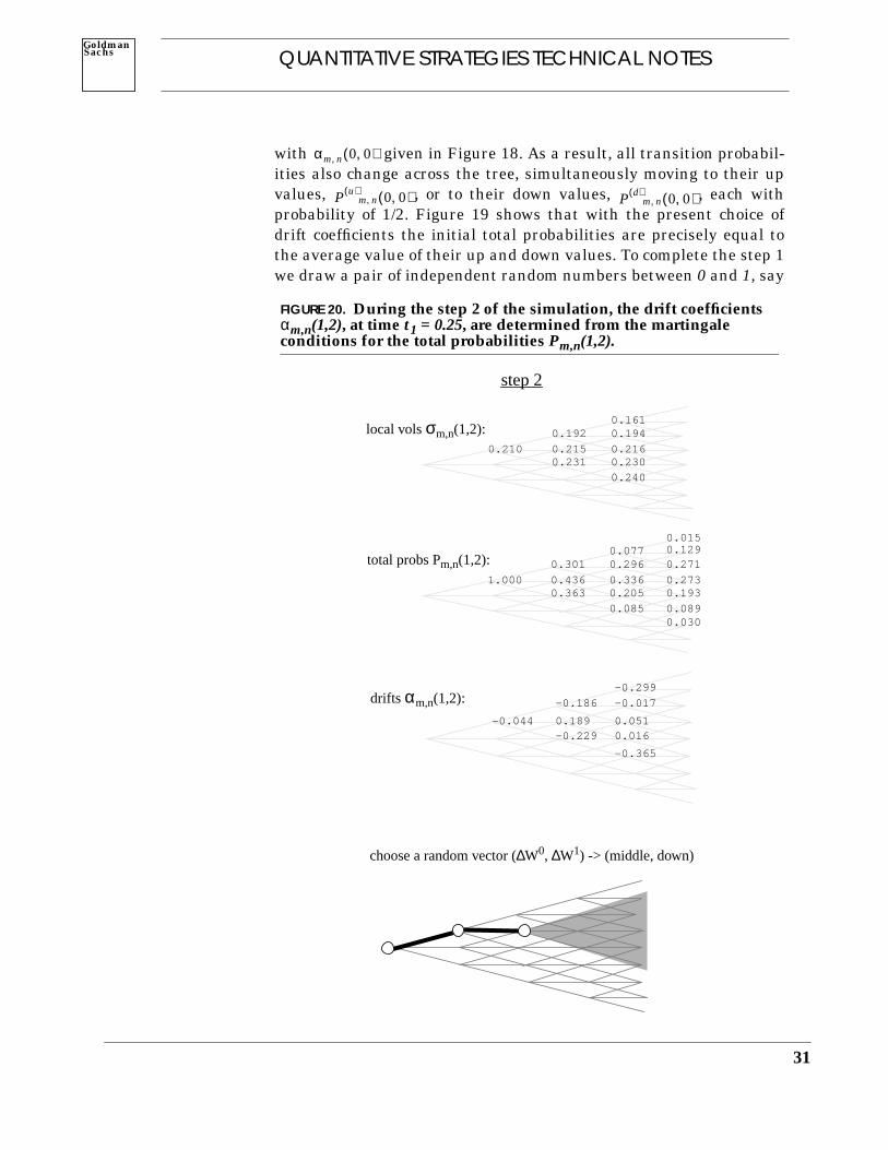
with given in Figure 18. As a result, all transition probabil-ities also change across the tree, simultaneously moving to their upvalues, , or to their down values, , each withprobability of 1/2. Figure 19 shows that with the present choice ofdrift coefficients the initial total probabilities are precisely equal tothe average value of their up and down values. To complete the step 1we draw a pair of independent random numbers between 0 and 1, say
αm n, 0 0,( )
P u( )m n, 0 0,( ) P d( )
m n, 0 0,( )
FIGURE 20. During the step 2 of the simulation, the drift coefficientsαm,n(1,2), at time t1 = 0.25, are determined from the martingaleconditions for the total probabilities Pm,n(1,2).
0.210 0.215 0.2160.231 0.230
0.192 0.1940.161
0.240
local volsσm,n(1,2):
0.089
1.000 0.436 0.336 0.2730.363 0.205 0.193
0.301 0.296 0.271
0.030
0.077 0.1290.015
0.085
total probs Pm,n(1,2):
-0.044 0.189 0.051-0.229 0.016
-0.186 -0.017
-0.299
-0.365
drifts αm,n(1,2):
choose a random vector (∆W0, ∆W1) -> (middle, down)
step 2
31
32
QUANTITATIVE STRATEGIES TECHNICAL NOTESSachsGoldman
(0.853, 0.612). Since 0.853 is greater than the sum of prevailingdown and middle probabilities, 0.493+0.232 = 0.725, as discussed inFigure 16 we move the index to the node (1,2). Also, since 0.612 isgreater than 1/2 we move all local volatilities to their up values,before we begin the next simulation step. The step 2 of the simula-
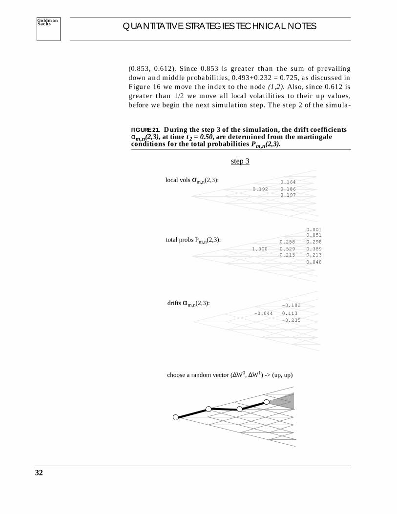
FIGURE 21. During the step 3 of the simulation, the drift coefficientsαm,n(2,3), at time t2 = 0.50, are determined from the martingaleconditions for the total probabilities Pm,n(2,3).
0.192 0.1860.197
0.164local volsσm,n(2,3):
0.048
1.000 0.529 0.3890.213 0.213
0.258 0.2980.0510.001
total probs Pm,n(2,3):
-0.044 0.113-0.235
-0.182drifts αm,n(2,3):
choose a random vector (∆W0, ∆W1) -> (up, up)
step 3

QUANTITATIVE STRATEGIES TECHNICAL NOTESGoldmanSachs
tion is precisely the same as step 1, except confined to the subtreethat begins at the node (1,2). As shown in Figure 20, again the mar-tingale conditions on the total probabilities are used tosolve for the drift coefficients at time t1 = 0.25, and thenthese coefficients, together with a pair of random numbers, are usedto determine jointly the new values for the index price and the future
Pm n, 1 2,( )αm n, 1 2,( )
FIGURE 22. During the step 4 of the simulation, the drift coefficientsαm,n(3,5), at time t3 = 0.75, are determined from the martingaleconditions for the total probabilities Pm,n(3,5).
0.180local volsσm,n(3,5):
0.183
1.000 0.5840.232
total probs Pm,n(3,5):
-0.044drifts αm,n(3,5):
choose a random vector (∆W0, ∆W1) -> (down, - )
step 4
33
34
QUANTITATIVE STRATEGIES TECHNICAL NOTESSachsGoldman
local volatilities. Steps 3 and 4 are also quite similar and theirresults have been shown in Figures 21 and 22, repsectively.
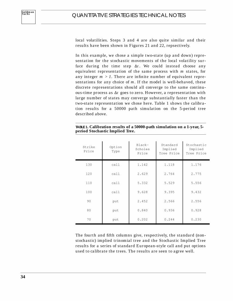
In this example, we chose a simple two-state (up and down) repre-sentation for the stochastic movements of the local volatility sur-face during the time step . We could instead choose anyequivalent representation of the same process with m states, forany integer m > 1. There are infinite number of equivalent repre-sentations for any choice of m. If the model is well-behaved, thesediscrete representations should all converge to the same continu-ous-time process as goes to zero. However, a representation withlarge number of states may converge substantially faster than thetwo-state representation we chose here. Table 1 shows the calibra-tion results for a 50000 path simulation on the 5-period treedescribed above.
TABLE 1. Calibration results of a 50000-path simulation on a 1-year, 5-period Stochastic Implied Tree.
The fourth and fifth columns give, respectively, the standard (non-stochastic) implied trinomial tree and the Stochastic Implied Treeresults for a series of standard European-style call and put optionsused to calibrate the trees. The results are seen to agree well.
StrikePrice
OptionType
Black-Scholes
Price
StandardImplied
Tree Price
StochasticImplied
Tree Price
130 call 1.142 1.118 1.176
120 call 2.629 2.764 2.775
110 call 5.332 5.529 5.556
100 call 9.628 9.395 9.432
90 put 2.452 2.566 2.556
80 put 0.840 0.936 0.928
70 put 0.202 0.244 0.230
∆t
∆t

QUANTITATIVE STRATEGIES TECHNICAL NOTESGoldmanSachs
Pricing of Some Contractswith Payoffs Based on RealizedVolatility
CAVIAT: Since the location of the nodes (i.e the state space) of thestochastic implied trinomial tree is fixed throughout, it may not bepossible to fit very large local volatilities, which may occur at variousnodes and at different times during the simulation, with transitionprobabilities which lie between 0 and 1. In such cases, we must over-write the unacceptable transition probabilities (or, equivalently, thelocal volatilities) at those nodes15. Even though, this overwrite proce-dure makes for an imperfect calibration to the initial smile (and, the-oretically, a violation of arbitrage), it must be diligently adhered to,in order to keep the simulation process meaningful. We can defineoverwrite ratio as the number of overwrites per future node, per sim-ulation path. In the previous example, the overwrite ratio for 5 peri-ods and 50000 paths is found to be 2.7%, indicating that only arelatively small portion of the calculated local volatilities have beenoverwritten.
Consider a realized variance forward contract16, defined as a forwardcontract on the realized variance of index returns, , with strikeprice K and payoff at the contract maturity. Table 2 showsthe valuation results for a 1-year realized variance contract with zerostrike price, using 20-period, 10000 path stochastic implied tree sim-ulations with four different volatility of volatility parameters θ = 0%,20%, 30%, 50%. To make the results more clear, we choose a flat ini-tial volatility smile with a constant implied volatility of 20% for allstandard European options. Also the discount rate and dividend yieldare both chosen to be zero.
TABLE 2. Prices of a zero-strike realized variance forward contract fordifferent values of the volatility of volatility parameter.
It is clear from this table that the price of a realized variance forwardcontract is independent of the volatility of volatility parameter, and is
15. This also occurs in the standard implied trees. See, for instance, Derman, Kaniand Chriss [1996].16. See also Investing in Volatility, Derman etal. [1996].
θ 0% 20% 30% 50%
price 399.81 400.37 401.10 400.69
Σ2
Σ2 K–( )
35

36
QUANTITATIVE STRATEGIES TECHNICAL NOTESSachsGoldman
what one would expect from a static 20% flat initial implied volatilitysurface. In fact, it can be shown that under very general conditions(see footnote 14) the price of this forward contract depends only onthe initial volatility surface and not on the specific stochastic aspectsof the volatility process. More precisely, it’s price equals the dis-counted value of the expected (equilibrium) total index return vari-ance during the life of the contract. As discussed earlier, thisexpectation is fully embodies in today’s local volatility surface. There-fore, we are able to price this forward contract by using an effectivetheory (θ = 0), as the second column in the table indicates. This isquite analogous to our ability to price index forwards contracts usingthe static initial forward curve without any specific knowledge of thestochastic behavior of the future index prices, or to price straightbonds using the initial yield curve with no specific knowledge of thebehavior of future interest rates.
Now consider a realized variance (call) option contract with strikeprice K whose payoff at maturity is given by . Table 3shows the valuation results for 1-year realized variance call optionswith different strike prices, under precisely the same conditions asbefore.
TABLE 3. Prices of realized variance call option contracts with differentstrike prices and volatility of volatility parameters.
According to this table the price of a realized variance option contractincreases with the volatility of volatility parameter. This resultshould be expected as most options’ prices increase when their under-lyer price becomes more volatile. Furthermore, like most options, thepricing and hedging of a realized variance option contract dependscrucially on our choice of the stochastic volatility model.
θ 0% 20% 30% 50%
400 0.00 48.336 65.784 95.742
500 0.00 14.745 31.221 56.096
600 0.00 3.391 11.780 25.211
700 0.00 0.203 1.682 4.654
Max Σ2 K– 0,( )
K

QUANTITATIVE STRATEGIES TECHNICAL NOTESGoldmanSachs
HEDGING THE INDEX ANDVOLATILITY RISKS IN STOCHASTICVOLATILITY MODELS
MORE REALISTIC STOCHASTICVOLATILITY MODELS
Appendix D gives conditions for the existence and uniqueness of anequivalent martingale measure in multi-factor stochastic volatilitymodels. Under these conditions the markets are complete and, given acontingent claim C, there exists an admissible self-financing tradingstrategy (Harrison and Pliska [1981]) involving the index S, the moneymarket account B, and (any) n different standard options , i =1,...,n, which replicate this contingent claim:
a.e.
This replication strategy is dynamical, so that the hedge ratios NB, NSand Ni, i = 1, ..,n, are in general functions of time and other dynamicalvariables.
To find the hedge ratios NS and Ni we must separately move the indexprice S and introduce n independent shocks Wi (possibly correspondingto the n independent factors) to the initial local volatility surface, andsubsequently reprice the contingent claim and the n hedge standardoptions. For the simple model in our examples, we find these hedgeratios from solving the following system of equations
This system has a unique solution if the sensitivity matrix on the righthand side is non-singular. This is true if , i.e when the sen-sitivity of the option to a parallel shift in the local volatility surface ispositive. This condition holds for any standard option with non-zerostrike price.
In the previous example, all instantaneous changes of the volatilitysurface are caused by a single source of randomness, a parallel shiftfactor. However, empirical analyses17 of the daily changes of the vola-tility surface for index options reveals other important sources of ran-domness. A more realistic stochastic volatility model may be, forexample, given by the following pair of stochastic differential equa-tions:
17. To be presented in an upcoming Quantitative Strategies Research Note.
Ci CKi Ti,=
NBB NSS NiCi
i 1=
n
∑+ + C=
1 C1∂ S∂⁄
0 C1∂ W1∂⁄
NS
N1
C∂ S∂⁄
C∂ W1∂⁄=
C1 W1∂⁄∂ 0>
dSS
------ µdt σdW0+=
dσ2K T, t S,( )
σ2K T, t S,( )
------------------------------- αK T, t S,( )dt θ1dW1 θ2e λ T t–( )– dW2 θ3e η K S–( )– dW3+ + +=
37

38
QUANTITATIVE STRATEGIES TECHNICAL NOTESSachsGoldman
SUMMARY
where and are all constants. The firstfactor has the same interpretation as before, whereas the second andthird factors may be interpreted as the term structure factor andskewness factor, respectively. The shocks to the local volatility surfaceresulting from these factors are shown in the figure below:
In this paper we discussed an arbitrage pricing approach to contin-gent claims valuation with stochastic volatility similar to the Heath-Jarrow-Morton (HJM) methodology for stochastic interest rates. Webegan with a continuous time economy with multiple factors, andposited a general multi-factor continuous time stochastic process forthe evolution of the local volatility surface. We characterized the con-ditions which guarantee absence of arbitrage opportunities amongthe various option and forward contracts defined on the underlyingindex. Under these conditions markets are complete and contingentclaim valuation is preference-free. However, these no-arbitrage condi-tions are non-linear and difficult to use in their continuous form. Wethen introduced the Stochastic Implied Tree as a discrete-timeframework for implementing our family of models. Starting from anyinitial node, we can guarantee absence of future arbitrages by choos-ing appropriate drift parameters for every future node. This proce-dure guarantees arbitrage-free future movements of the index andlocal volatility surface in the discrete-time world defined by the sto-chastic implied tree. We can use Stochastic Implied Trees to pricecontingent claims with payoffs which depend on the index and indexvolatility, when the volatility surface is skewed and stochastic. Theresulting contingent claim prices are independent of the marketprices of risk. They are also consistent with the current market pricesof all standard options and forwards defined on the underlying indexand with the absence of any future arbitrage opportunities.
σ t( ) σt St, t St,( )= θ1 θ2 θ3 λ η, , , ,
(a) parallel shift (b) term structure (c) skewness
K
T
σK,T σK,T σK,T
K K
T T

QUANTITATIVE STRATEGIES TECHNICAL NOTESGoldmanSachs
APPENDIX A: ExpectationDefinitions of Local Volatility
This appendix provides expectation definitions for local volatility. Itbegins with Equation 2 as the definition of local volatility and derivesthe expectation relationships between local volatilities and futureinstantaneous volatilities, given the assumption that the equivalentmartingale measure exists.
Under the equivalent martingale measure, the index price evolutionis given by the stochastic differential equation
(EQ 58)
where the riskless discount rate r and continuously compounded div-idend yield δ are assumed to be constant, is the instantaneous vol-atility at time t and is a standard Brownian motion underthis measure, as discussed in the text. Let denote the expec-tation corresponding to this measure, given the information availableat time t (with the index level at S = St). Aside from the spot indexlevel, the information at time t generally includes the past index lev-els, the values of the n (independent) stochastic factors Wi (governingthe stochastic behavior of volatility) and their past histories. Underthe equivalent martingale measure rescaled option prices are mar-tingales. Therefore, the price, , at time t and market level Sof a standard European-style (call) option, with strike K and matu-rity T, with terminal value is given by
(EQ 59)
Differentiating this equation once with respect to K gives
(EQ 60)
where θ(.) is the Heaviside function. Differentiating twice withrespect to K gives
(EQ 61)
where δ(.) is the Dirac delta function. Lastly, differentiating withrespect to T gives
(EQ 62)
dSt
St-------- r δ–( )dt σtdZt+=
σt
Z W0
=
E Et S,=
CK T, t S,( )
CK T, T ST,( ) ST K–( ) +=
CK T, t S,( ) e r T t–( )– E ST K–( ) +[ ]=
K∂∂CK T, e– r T t–( )– E θ ST K–( )[ ]=
K2
2
∂∂ CK T, e r T t–( )– E δ ST K–( )[ ]=
T∂∂CK T, r– CK T, e r T t–( )–
T∂∂ E ST K–( ) +[ ]+=
39
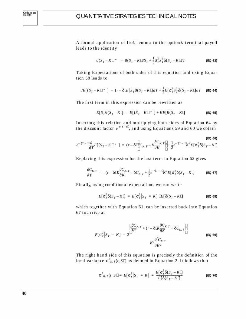
40
QUANTITATIVE STRATEGIES TECHNICAL NOTESSachsGoldman
A formal application of Ito’s lemma to the option’s terminal payoffleads to the identity
(EQ 63)
Taking Expectations of both sides of this equation and using Equa-tion 58 leads to
(EQ 64)
The first term in this expression can be rewritten as
(EQ 65)
Inserting this relation and multiplying both sides of Equation 64 bythe discount factor , and using Equations 59 and 60 we obtain
(EQ 66)
Replacing this expression for the last term in Equation 62 gives
(EQ 67)
Finally, using conditional expectations we can write
(EQ 68)
which together with Equation 61, can be inserted back into Equation67 to arrive at
(EQ 69)
The right hand side of this equation is precisely the definition of thelocal variance , as defined in Equation 2. It follows that
(EQ 70)
d ST K–( ) + θ ST K–( )dST12---σT
2 ST2 δ ST K–( )dT+=
dE ST K–( ) +[ ] r δ–( )E STθ ST K–( )[ ]dT 12---E σT
2 ST2 δ ST K–( )[ ]dT+=
E STθ ST K–( )[ ] E ST K–( ) +[ ] KE θ ST K–( )[ ]+=
e r T t–( )–
e r T t–( )–
T∂∂ E ST K–( ) +[ ] r δ–( ) CK T, K
K∂∂CK T,–
1
2---e r T t–( )– K2E σT
2 δ ST K–( )[ ]+=
T∂∂CK T, r δ–( )K–
K∂∂CK T, δCK T,–
12---e r T t–( )– K2E σT
2 δ ST K–( )[ ]+=
E σT2 δ ST K–( )[ ] E σT
2 ST[ K ] E δ ST K–( )[ ]⋅= =
E σT2 ST[ K ] 2
T∂∂CK T, r δ–( )K
K∂∂CK T, δCK T,+ +
K2
K2
2
∂∂ CK T,
-------------------------------------------------------------------------------------= =
σ2K T, t S,( )
σ2K T, t S,( ) E σT
2 ST[ K ]E σT
2 δ ST K–( )[ ]E δ ST K–( )[ ]----------------------------------------= = =

QUANTITATIVE STRATEGIES TECHNICAL NOTESGoldmanSachs
The local variance is, therefore, the conditional expectationof the instantaneous variance of index returns at the future time T,contingent on index level ST being equal to K. If the instantaneousindex volatility is only a function of the spot index level and time, i.e.if σt = σ(St , t), then
(EQ 71)
Since the right hand side is independent of t and S, in this case thelocal volatility surface remains static as time t evolves and indexlevel S changes. This situation corresponds to an effective theorywhere all sources of volatility uncertainty, other than the future timet and the future index level S, are effectively averaged out of the the-ory, leaving an effective volatility which is only a function of t and S.
In the general stochastic setting the dynamics of local volatilities isdescribed by the stochastic differential equation
(EQ 72)
As discussed in the text, , i = 0, ...,n, are independent Brownianmotions under the equivalent martingale measure and the volatilitycoefficients are some given functions of time t, index level S andfactor values Wi
t , or the past histories of these variables. The driftcoefficients have similar dependencies, but are constrainedby the requirement of no-arbitrage. In an effective theory
for all values of t and S, as seen by Equation 71, thusthe drift and volatility coefficients are all identically equal to zero.
The denominator on the right hand side of Equation 70 is the totaltransition probability (see Equation 39):
(EQ 73)
Since , for all values of K and T, are jointly martingales underthe equivalent martingale measure, the stochastic differential equa-tion governing their evolution has the form
(EQ 74)
σ2K T, t S,( )
σ2K T, t S,( ) E σT
2 ST[ K ] E σ2 ST T,( ) ST[ K ] σ2 K T,( )= = = = =
dσ2K T, t S,( )
σ2K T, t S,( )
------------------------------- αK T, t S,( )dt θiK T, t S,( )dWi
t
i 0=
n
∑+=
Wi
θiK T,
αK T, t S,( )
dσ2K T, t S,( ) 0=
PK T, t S,( )
PK T, t S,( ) E δ ST K–( )[ ]=
PK T,
dPK T, t S,( )PK T, t S,( )---------------------------- ζi
K T, t S,( )dWit
i 0=
n
∑=
41

42
QUANTITATIVE STRATEGIES TECHNICAL NOTESSachsGoldman
The numerator on the right hand side of Equation 70 is also a mar-tingale under this measure. Therefore, by taking differentials of bothsides of this equation and applying Ito’s lemma we find that
(EQ 75)
Let us define a new measure, , specifically depend-ing on K and T. From Equations 72 and 75 we observe that under thisnew measure local variance is a martingale, i.e
(EQ 76)
We call this measure the K-strike and T-maturity forward risk-adjusted measure in analogy with T-maturity forward risk-neutralmeasure in interest rates (see Jamshidian [1993]). Lettingdenote expectations with respect to this new measure, we can writeEquation 70 as
(EQ 77)
Therefore, in the K-strike and T-maturity forward risk-adjusted mea-sure the local variance is the expectation of future spot vari-ances at time T. This is analogous to the similar situation ininterest rate world where the forward rate is the T-maturity for-ward risk-adjusted expectation of the future spot rates at time T.
αK T, ζiK T, θi
K T,
i 0=
n
∑+ 0=
dWi
dWi ζi
K T, dt–=
σ2K T,
dσ2K T, t S,( )
σ2K T, t S,( )
------------------------------- θiK T, t S,( )dW
it
i 0=
n
∑=
E K T,( ) …[ ]
σ2K T, E K T,( ) σT
2[ ]=
σ2K T,
σT2
f T
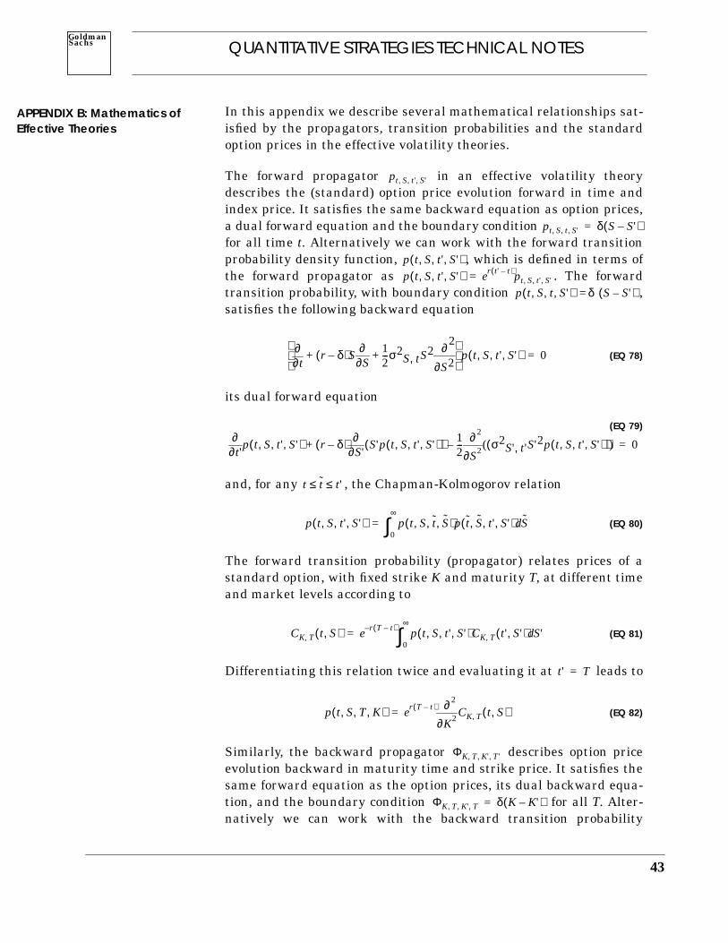
QUANTITATIVE STRATEGIES TECHNICAL NOTESGoldmanSachs
APPENDIX B: Mathematics ofEffective Theories
In this appendix we describe several mathematical relationships sat-isfied by the propagators, transition probabilities and the standardoption prices in the effective volatility theories.
The forward propagator in an effective volatility theorydescribes the (standard) option price evolution forward in time andindex price. It satisfies the same backward equation as option prices,a dual forward equation and the boundary conditionfor all time t. Alternatively we can work with the forward transitionprobability density function, , which is defined in terms ofthe forward propagator as . The forwardtransition probability, with boundary condition ,satisfies the following backward equation
(EQ 78)
its dual forward equation
(EQ 79)
and, for any , the Chapman-Kolmogorov relation
(EQ 80)
The forward transition probability (propagator) relates prices of astandard option, with fixed strike K and maturity T, at different timeand market levels according to
(EQ 81)
Differentiating this relation twice and evaluating it at leads to
(EQ 82)
Similarly, the backward propagator describes option priceevolution backward in maturity time and strike price. It satisfies thesame forward equation as the option prices, its dual backward equa-tion, and the boundary condition for all T. Alter-natively we can work with the backward transition probability
pt S t' S', , ,
pt S t S', , , δ S S'–( )=
p t S t' S', , ,( )p t S t' S', , ,( ) er t' t–( )pt S t' S', , ,=
p t S t S', , ,( ) δ S S'–( )=
t∂∂ r δ–( )S
S∂∂ 1
2---σ2
S t, S2S2
2
∂∂
+ +
p t S t' S', , ,( ) 0=
t'∂∂ p t S t' S', , ,( ) r δ–( )
S'∂∂ S'p t S t' S', , ,( )( ) 1
2---
S2
2
∂∂ σ2
S' t', S'2p t S t' S', , ,( )( )( )–+ 0=
t t t'≤ ≤
p t S t' S', , ,( ) p t S t S, , ,( )p t S t' S', , ,( ) Sd0
∞
∫=
CK T, t S,( ) e r T t–( )– p t S t' S', , ,( )CK T, t' S',( ) S'd0
∞
∫=
t' T=
p t S T K, , ,( ) er T t–( )
K2
2
∂∂ CK T, t S,( )=
ΦK T K' T', , ,
ΦK T K' T, , , δ K K'–( )=
43

44
QUANTITATIVE STRATEGIES TECHNICAL NOTESSachsGoldman
density function, , which is defined in terms of the back-ward propagator as . The backwardtransition probability density function, with the boundary condition
, satisfies the following forward equation
(EQ 83)
its dual backward equation
(EQ 84)
and, for any , the chapman-Kolmogorov relation
(EQ 85)
The backward transition probability (propagator) relates prices ofstandard options, with different strikes and maturities, at a fixedtime t, , and market level S according to
(EQ 86)
Differentiating this relation twice and evaluating it at leads to
(EQ 87)
Φ K T K' T', , ,( )Φ K T K' T', , ,( ) eδ T T'–( )ΦK T K' T', , ,=
Φ K T K' T, , ,( ) δ K K'–( )=
T∂∂ r δ–( )K
K∂∂ 1
2---σ2
K T, K2K2
2
∂∂
–+
Φ K T K' T', , ,( ) 0=
T'∂∂ Φ K T K' T', , ,( ) r δ–( )
K'∂∂ K'Φ K T K' T', , ,( )( )
12---
K'2
2
∂∂ σ2
K' T', K'2Φ K T K' T', , ,( )( )+ + 0=
T' T T≤ ≤
Φ K T K' T', , ,( ) Φ K T K T, , ,( )Φ K T K' T', , ,( ) Kd0
∞
∫=
t T' T≤ ≤
CK T, t S,( ) e δ T T'–( )– Φ K T K' T', , ,( )CK' T', t S,( )0
∞
∫=
T' t=
Φ K T S t, , ,( ) eδ T t–( )
S2
2
∂∂ CK T, t S,( )=

QUANTITATIVE STRATEGIES TECHNICAL NOTESGoldmanSachs
APPENDIX C: Local VolatilityVariational Formulas inEffective Volatility Theories
In this appendix we derive variational formulas describing sensitiv-ity of the transition probabilities (propagators) to a specific local vola-tility on the volatility surface. We work within the context of effectivetheories, (formally) changing the local volatility corresponding to asingle future time and market level, while leaving all other local vol-atilities unchanged.
We begin by studying the relationship between transition probabili-ties and local volatilities in a discrete time setting. We then take thecontinuous-time limit by letting the spacing go to zero. Consider oneperiod forward transition probabilities p*u, p*m and p*d, from theindex level S* at time t* to the three nearby index levels S*u, S*mand S*d at time t*+ ∆t*, as shown in the figure below:
Let denote the one-step forward price andthe local volatility, corresponding to the initial node (t*,S*). The threetransition probabilities in the figure add up to one, and are furtherconstrained by the forward and volatility conditions, i.e
(EQ 88)
(EQ 89)
(EQ 90)
We can solve these expressions for transition probabilities in terms ofthe local volatility. The results are
(EQ 91)
(EQ 92)
and .
S*
S*u
S*m
S*d
p*u
p*m
p*d
F*
F∗ S∗e r δ–( )∆t∗= σ∗ σS∗ t∗,=
p∗u p∗m p∗d+ + 1=
p∗uS∗u p∗mS∗m p∗dS∗d+ + F∗=
p∗u S∗u F∗–( )2p∗m S∗m F∗–( )2
p∗d S∗d F∗–( )2+ + F∗2σ∗2∆t∗=
p∗uF∗ S∗m–( ) F∗ S∗d–( )
S∗u S∗m–( ) S∗u S∗d–( )----------------------------------------------------------
F∗2
S∗u S∗m–( ) S∗u S∗d–( )----------------------------------------------------------σ∗2∆t∗+=
p∗dF∗ S∗m–( ) F∗ S∗u–( )
S∗m S∗d–( ) S∗u S∗d–( )----------------------------------------------------------
F∗2
S∗m S∗d–( ) S∗u S∗d–( )----------------------------------------------------------σ∗2∆t∗+=
p∗m 1 p∗u p∗d––=
45

46
QUANTITATIVE STRATEGIES TECHNICAL NOTESSachsGoldman
Now consider the forward transition probability , describ-ing the total probability that starting with the level S at time t theindex will move to the level S' at the future time t', in the effectivetheory context. We can isolate the sensitivity of this transition proba-bility to a specific local volatility , corresponding to the futuretime and future market level , using the Chapman-Kol-mogorov relation of Equation 80. In discrete-time this contribution isisolated in the following figure:
This figure describes the following decomposition of the total transi-tion probability:
(EQ 93)
terms with no sensitivity to σS*,t*
Taking the variational derivative with respect to gives
(EQ 94)
p t S t' S', , ,( )
σS∗ t∗,t t∗ t'≤ ≤ S∗
S*u
S*m
S*d
p*u
p*m
p*dS*
t t* t*+∆t* t'
S'S
p t S t' S', , ,( ) p t S t∗ S∗, , ,( )p∗up t∗ ∆t∗+ S∗u t' S', , ,( ) +=
p t S t∗ S∗, , ,( )p∗mp t∗ ∆t∗+ S∗m t' S', , ,( ) +
p t S t∗ S∗, , ,( )p∗dp t∗ ∆t∗+ S∗d t' S', , ,( ) +
σ2S∗ t∗,
δp t S t' S', , ,( )δσ2
S∗ t∗,
--------------------------------- p t S t∗ S∗, , ,( )δp∗u
δσ2S∗ t∗,
-------------------
p t∗ ∆t∗+ S∗u t' S', , ,( ) +=
p t S t∗ S∗, , ,( )δp∗m
δσ2S∗ t∗,
-------------------
p t∗ ∆t∗+ S∗m t' S', , ,( ) +
p t S t∗ S∗, , ,( )δp∗d
δσ2S∗ t∗,
-------------------
p t∗ ∆t∗+ S∗d t' S', , ,( )
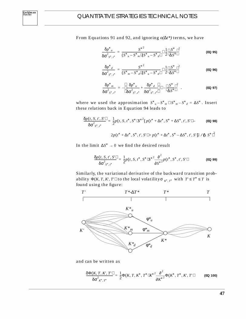
QUANTITATIVE STRATEGIES TECHNICAL NOTESGoldmanSachs
From Equations 91 and 92, and ignoring o(∆t*) terms, we have
(EQ 95)
(EQ 96)
. (EQ 97)
where we used the approximation . Insertthese relations back in Equation 94 leads to
(EQ 98)
In the limit we find the desired result
(EQ 99)
Similarly, the variational derivative of the backward transition prob-ability to the local volatility with isfound using the figure:
and can be written as
(EQ 100)
δp∗u
δσ2S∗ t∗,
-------------------S∗2
S∗u S∗m–( ) S∗u S∗d–( )----------------------------------------------------------
12---
S∗∆S∗----------
2∼=
δp∗d
δσ2S∗ t∗,
-------------------S∗2
S∗m S∗d–( ) S∗u S∗d–( )----------------------------------------------------------
12---
S∗∆S∗----------
2
∼=
δp∗m
δσ2S∗ t∗,
-------------------δp∗u
δσ2S∗ t∗,
-------------------δp∗d
δσ2S∗ t∗,
-------------------+
–S∗
∆S∗---------- 2
–∼=
S∗u S∗m– S∗m S∗d–∼ ∆S∗=
δp t S t' S', , ,( )δσ2
S∗ t∗,
---------------------------------12---p t S t∗ S∗, , ,( )S∗2
p t∗ ∆t∗+ S∗ ∆S∗+ t' S', , ,( ) –{=
2p t∗ ∆t∗+ S∗ t' S', , ,( ) p t∗ ∆t∗+ S∗ ∆S∗– t' S', , ,( ) } ∆S∗( )⁄ 2+
∆S∗ 0→
δp t S t' S', , ,( )δσ2
S∗ t∗,
---------------------------------12---p t S t∗ S∗, , ,( )S∗2
S∗2
2
∂∂ p t∗ S∗ t' S', , ,( )=
Φ K T K' T', , ,( ) σK∗ T∗, T' T∗ T≤ ≤
K*u
K*m
K*d
φ*m
φ*d
K*
TT*T*-∆T*T'
K'K
φ*u
δΦ K T K' T', , ,( )δσ2
K∗ T∗,
----------------------------------------12---Φ K T K∗ T∗, , ,( )K∗2
K∗2
2
∂∂ Φ K∗ T∗ K' T', , ,( )=
47
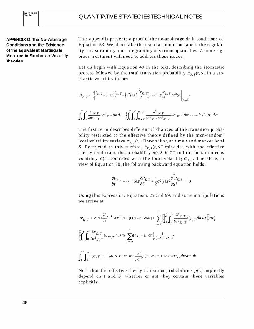
48
QUANTITATIVE STRATEGIES TECHNICAL NOTESSachsGoldman
APPENDIX D: The No-ArbitrageConditions and the Existenceof the Equivalent MartingaleMeasure in Stochastic VolatilityTheories
This appendix presents a proof of the no-arbitrage drift conditions ofEquation 53. We also make the usual assumptions about the regular-ity, measurability and integrability of various quantities. A more rig-orous treatment will need to address these issues.
Let us begin with Equation 40 in the text, describing the stochasticprocess followed by the total transition probability in a sto-chastic volatility theory:
The first term describes differential changes of the transition proba-bility restricted to the effective theory defined by the (non-random)local volatility surface prevailing at time t and market levelS. Restricted to this surface, coincides with the effectivetheory total transition probability and the instantaneousvolatility coincides with the local volatility . Therefore, inview of Equation 78, the following backward equation holds:
Using this expression, Equations 25 and 99, and some manipulationswe arrive at
Note that the effective theory transition probabilities p(..) implicitlydepend on t and S, whether or not they contain these variablesexplicitly.
PK T, t S,( )
dPK T, t∂
∂PK T, µ t( )SS∂
∂PK T, 12---σ2 t( )S2
S2
2
∂
∂ PK T,+ +
dt σ t( )SS∂
∂PK T, dW0 t( )+
t S,( )= +
δPK T,δσ2
K' T',------------------------ σ2
K' T',d K'd T'd0
∞
∫t
T
∫ 12---
δ2PK T,
δσ2K' T', δσ2
K'' T'',--------------------------------------------------- σ2
K' T',d σ2K'' T'',d K'd K''d T' T''dd
0
∞
∫0
∞
∫t
T
∫t
T
∫+
σK T, t S,( )PK T, t S,( )
p t S K T, , ,( )σ t( ) σt S,
t∂∂PK T, r δ–( )S
S∂∂PK T, 1
2---σ2 t( )S2
S2
2
∂∂ PK T,+ + 0=
dPK T, σ t( )SS∂
∂PK T, dW0 t( ) µ t( ) r– δ+( )dt+[ ]δPK T,
δσ2K' T',
-----------------------θK' T',i
K'd T'd0
∞
∫t
T
∫
dWti
i 0=
n
∑+=
δPK T,δσ2
K' T',-----------------------
0
∞
∫ α[ K' T', t S,( ) θiK' T', t S,( ) 1
p t S T' K', , ,( )--------------------------------- ×
i 0=
n
∑+t
T
∫
θiK'' T'', t S,( )p t S T'' K'', , ,( )K''2
K''2
2
∂∂ p T'' K, '' T' K', ,( ) K'd ' T'' } ] K'd T'dd ) td
0
∞
∫t
T'
∫
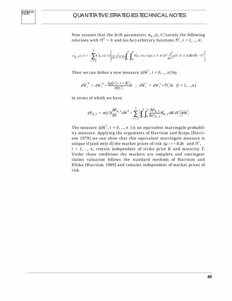
QUANTITATIVE STRATEGIES TECHNICAL NOTESGoldmanSachs
Now assume that the drift parameters satisfy the followingrelations with and (so far) arbitrary functions , i = 1, .., n:
Then we can define a new measure { , i = 0, .., n} by
; (i = 1, ..,n)
in terms of which we have
The measure { , i = 0, .., n } is an equivalent martingale probabil-ity measure. Applying the arguments of Harrison and Kreps [Harri-son 1979] we can show that this equivalent martingale measure isunique if (and only if) the market prices of risk and ,i = 1, .., n, remain independent of strike price K and maturity T.Under these conditions the markets are complete and contingentclaims valuation follows the standard methods of Harrison andPliska [Harrison 1989] and remains independent of market prices ofrisk.
σK T, t S,( )Π0 0= Πi
σK T, t S,( ) θiK T, t S,( ) 1
p t S T K, , ,( )------------------------------ θiK' T', t S,( )p t S T' K', , ,( )K2'
K'2
2
∂∂ p T' K', T K, ,( ) Kd ' T'd
0
∞
∫t
T'
∫ Πi–
i 0=
n
∑–=
dWi
dWt0
dWt0 µ t( ) r– δ+( )
σ t( )---------------------------------dt+= dWti
dWti Πt
idt+=
dPK T, σ t( )SS∂
∂PK T, dW0 δPK T,
δσ2K' T',
------------------θK' T',i K'd T'd
0
∞
∫t
T
∫ dWt
i
i 0=
n
∑+=
dWi
µ r– δ+( ) σ⁄ Πi
49
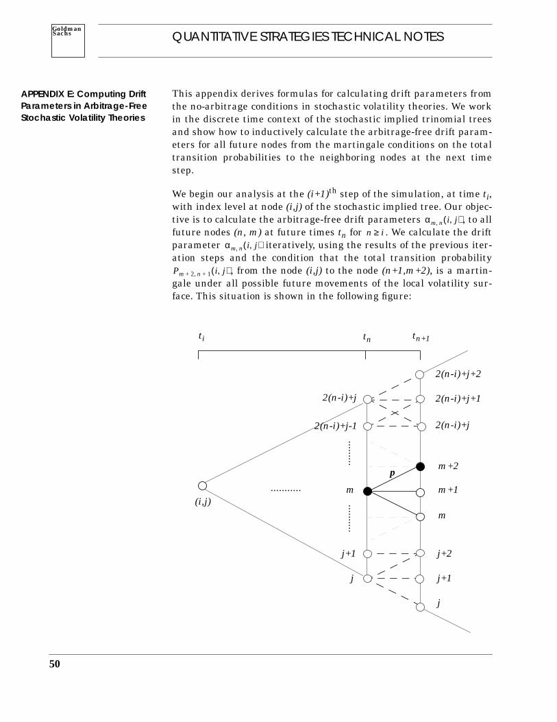
50
QUANTITATIVE STRATEGIES TECHNICAL NOTESSachsGoldman
APPENDIX E: Computing DriftParameters in Arbitrage-FreeStochastic Volatility Theories
This appendix derives formulas for calculating drift parameters fromthe no-arbitrage conditions in stochastic volatility theories. We workin the discrete time context of the stochastic implied trinomial treesand show how to inductively calculate the arbitrage-free drift param-eters for all future nodes from the martingale conditions on the totaltransition probabilities to the neighboring nodes at the next timestep.
We begin our analysis at the (i+1)th step of the simulation, at time ti,with index level at node (i,j) of the stochastic implied tree. Our objec-tive is to calculate the arbitrage-free drift parameters , to allfuture nodes (n, m) at future times tn for . We calculate the driftparameter iteratively, using the results of the previous iter-ation steps and the condition that the total transition probability
, from the node (i,j) to the node (n+1,m+2), is a martin-gale under all possible future movements of the local volatility sur-face. This situation is shown in the following figure:
αm n, i j,( )n i≥
αm n, i j,( )
Pm 2+ n 1+, i j,( )
(i,j)
2(n-i)+j
j
2(n-i)+j-1
2(n-i)+j+2
2(n-i)+j+1
2(n-i)+j
m+2
m+1
m
j+2
j+1
j
m
j+1
ti tn tn+1
...........
...................
p

QUANTITATIVE STRATEGIES TECHNICAL NOTESGoldmanSachs
The figure shows the subtree which starts at the initial node (i,j). Allthe future movements of the index and local volatilities will be con-fined to the nodes of this subtree. Our iteration for calculating driftparameters for all subtree nodes begins with the calculationof the drift parameter at the initial node, , and continues for-ward to subsequent time steps beginning with the highest node ateach time step.
To make matter simple, for now let us assume that the only possiblemovements of the local volatility surface during the next instant ∆tare up or down (proportionately), with some constant volatility , asin our example in the text, i.e
Suppose that we have calculated the drift parameters for every nodebefore time tn, and also for every nodes at time tn which lies abovethe node (n,m), shown in dark in the figure. We must now calculate
from the previously known quantities and the martingalecondition on the total probability , of arriving at the node(n+1, m+2) at the next time step. We can decompose the contributionsto this probability into two components as follows:
As in the figure, p denotes the one period up transition probabilityfrom the node (n,m) to the node (n+1, m+2). The first term describesthe contribution of the node (n,m) to the total transition probability,stemming from all the paths which go through this node before arriv-ing at (n+1,m+2). The second term describes the contribution of allthe nodes lying above the node (n,m) to this transition probability.
Consider now the next instant ∆t in time where all future local vola-tilities will simultaneously move either to their up state, ,or to their down state . Since transition probabilities aredirect functions of local volatilities, then all probabilities will alsosimultaneously move to their up or down states, i.e
αm n, i j,( )α j i, i j,( )
θ
σ u d,( )m n, i j,( ) σm n, i j,( ) αm n, i j,( ) 1
2---θ2–
∆t θ ∆t±
exp=
αm n, i j,( )Pm 2+ n 1+, i j,( )
Pm 2 n 1+,+ i j,( ) Pm n, i j,( )p Λm n, i j,( )+=
σ u( )m n, i j,( )
σ d( )m n, i j,( )
P u d,( )m 2 n 1+,+ i j,( ) P u d,( )
m n, i j,( )p u d,( ) Λ u d,( )m n, i j,( )+=
51

52
QUANTITATIVE STRATEGIES TECHNICAL NOTESSachsGoldman
The quantities and depend on drift parame-ters and other quantities known from the previous iteration steps,but remain unknown as they depend on the unknown driftparameter . We have previously discussed the structure ofthis dependence in Equations 91 and 92. The one period transitionprobability depends linearly on the local variance , i.e
, with coefficients A and B depending only on theposition of the nodes, which are fixed and known. Hence
Using this and previous relations, we can now determine theunknown drift parameter from the martingale condition forthe (known) total probability :
Therefore the desired formula is
This result can be readily extended to the cases where the local vola-tility surface can move to any number (more than two) of possiblestates during a time step, has multiple stochastic factors, or has fac-tor volatilities which are more complicated functions of time, marketlevel, factor values or their past histories.
P u d,( )m n, i j,( ) Λ u d,( )
m n, i j,( )
p u d,( )
αm n, i j,( )
p σ2m n, i j,( )
p A Bσ2m n, i j,( )+=
p u d,( ) A Bσ u d,( )2m n, i j,( )+= =
A Bσ2m n, i j,( ) 2 αm n, i j,( ) 1
2---θ2–
∆t 2θ ∆t±
exp+=
αm n, i j,( )Pm 2+ n 1+, i j,( )
Pm 2+ n 1+, i j,( ) 12--- P u( )
m 2+ n 1+, i j,( ) P d( )m 2+ n 1+, i j,( )+{ }=
12--- P u( )
m n, i j,( )p u( ) P d( )m n, i j,( )p d( ) Λ+
u( )m n, i j,( ) Λ d( )
m n, i j,( )+ +{ }=
12--- P u( )
m n, i j,( ) P d( )m n, i j,( )+[ ]A Λ u( )
m n, i j,( ) Λ d( )m n, i j,( )+ +{ } +=
12---Bσ2
m n, i j,( )e θ2∆t– P u( )m n, i j,( )e2θ ∆t P d( )
m n, i j,( )e 2θ ∆t–+[ ] 2αm n, i j,( )∆t{ }exp
αm n, i j,( )Pm 2+ n 1+, i j,( ) 1
2--- P
u( )m n, i j,( ) P
d( )m n, i j,( )+[ ]A Λ u( )
m n, i j,( ) Λ d( )m n, i j,( )+ +
–
12---Bσ2
m n, i j,( )eθ2∆t–
Pu( )
m n, i j,( )e2θ ∆t
Pd( )
m n, i j,( )e2θ ∆t–
+
-----------------------------------------------------------------------------------------------------------------------------------------------------------------------------------------------------------------------------------------log
2∆t( )⁄=

QUANTITATIVE STRATEGIES TECHNICAL NOTESGoldmanSachs
REFERENCES
Black, F. and M. Scholes (1973). The Pricing of Options and Corpo-rate Liabilities, Journal of Political Economy, Vol. 81, 637-654.
Black, F., E. Derman and W. Toy (1990). A One-Factor Model of Inter-est Rates and Its Application to Treasury Bond Options, FinancialAnalyst Journal, 817, 33-39.
Breeden, D. and R. Litzenberger (1978). The Pricing of State-Contin-gent Claims Implicit in Option Prices, Journal of Business, Vol. 51,621-651.
Cox, J., J. E. Ingersoll and S. Ross (1985). A Theory of the TermStructure of Interest Rates, Econometrica, Vol. 53, No. 2, 385-407.
Cox. J. and S. Ross (1976). The Valuation of Options for AlternativeStochastic Processes, Journal of Financial Economics, Vol. 3, 145-166.
Cox, J., S. Ross and M. Rubinstein (1979). Option Pricing: A Simpli-fied Approach, Journal of Financial Economics, Vol. 7, 229-263.
Derman, E. and I. Kani (1994). Riding on a Smile. RISK 7, No. 2, 32-39.
Derman, E., I. Kani and N. Chriss (1996). Implied Trinomial Trees ofthe Volatility Smile, Journal of Derivatives, Vol. 3, No. 4, 7-22.
Dupire, B. (1993). Model Art. RISK 6, No. 9, 118-124.
Dupire, B. (1994). Pricing with a Smile. RISK 7, No. 1, 18-20.
Eisenberg L. and R. Jarrow (1994). Option Pricing With Random Vol-atilities in Complete Markets, Review of Quantitative Finance andAccounting, Vol. 4, 5-17.
Harrison, J. M. and D. Kreps (1979). Martingales and Arbitrage inMultiperiod Securities Markets, Journal of Economic Theory, Vol. 20,381-408.
Harrison, J. M. and S. Pliska (1981). Martingales and StochasticIntegrals in the Theory of Continuous Trading. Stochastic Processesand Their Applications, Vol. 20, 215-260.
Heath, D., R. Jarrow and A. Morton (1992). Bond Pricing and TheTerm Structure of Interest Rates: A New Methodology for ContingentClaims Valuation, Econometrica, Vol. 60, No. 1, 77-105.
53

54
QUANTITATIVE STRATEGIES TECHNICAL NOTESSachsGoldman
Ho, T. S. Y. and S. B. Lee (1986). Term Structure Movements andPricing Interest Rate Contingent Claims, The Journal of Finance,Vol. 41, No. 5, 1011-1029.
Hull, J. and A. White (1987). The Pricing of Options on Assets WithStochastic Volatilities, Journal of Finance, Vol. 42, 271-301.
Jamshidian, F. (1993). Option and Futures Evaluation with Deter-ministic Volatilities, Mathematical Finance, Vol. 3, No. 2, 149-159.
Johnson, H. and D. Shanno (1987). Option Pricing When Variance isChanging, Journal of Financial and Quantitative Analysis, Vol. 22,143-153.
Kani, I., E. Derman and M. Kamal (1996). Trading and HedgingLocal Volatility, Quantitative Strategies Research Notes, GoldmanSachs & Co.
Merton, R. (1973). Theory of Rational Option Pricing, Bell Journal ofEconomics and Management Science, Vol. 4, 141-183.
Rubinstein, M.E. (1994). Implied Binomial Trees, Journal of Finance,Vol. 69, 771-818.
Stein, E. and J. Stein (1991). Stock Price Distribution With Stochas-tic Volatility: An Analytical Approach, The Review of Financial Stud-ies, Vol 4, No. 4, 727-752.
Vasicek, O. A. (1977). An Equilibrium Characterization of the TermStructure, Journal of Financial Economics Vol. 5, 177-188.
Wiggins, J. (1987). Option Values Under Stochastic Volatility: Theoryand Empirical Estimates, Journal of Financial Economics, Vol. 19,351-372.

QUANTITATIVE STRATEGIES TECHNICAL NOTESGoldmanSachs
SELECTED QUANTITATIVE STRATEGIES PUBLICATIONS
June 1990 Understanding Guaranteed Exchange-RateContracts In Foreign Stock InvestmentsEmanuel Derman, Piotr Karasinskiand Jeffrey S. Wecker
March 1992 Pay-On-Exercise OptionsEmanuel Derman and Iraj Kani
June 1993 The Ins and Outs of Barrier OptionsEmanuel Derman and Iraj Kani
January 1994 The Volatility Smile and Its Implied TreeEmanuel Derman and Iraj Kani
May 1994 Static Options ReplicationEmanuel Derman, Deniz Ergenerand Iraj Kani
May 1995 Enhanced Numerical Methods for Optionswith BarriersEmanuel Derman, Iraj Kani, Deniz Ergenerand Indrajit Bardhan
December 1995 The Local Volatility SurfaceEmanuel Derman, Iraj Kani and Joseph Z. Zou
February 1996 Implied Trinomial Trees of the Volatility SmileEmanuel Derman, Iraj Kani and Neil Chriss
August 1996 Trading and Hedging Local VolatilityIraj Kani, Emanuel Derman and Michael Kamal
October 1996 Investing in VolatilityEmanuel Derman, Michael Kamal, Iraj Kani,John McClure, Cyrus Pirasteh and Joseph Zou
55