remote sensing

Article

Quantitative Retrieval of Organic Soil Propertiesfrom Visible Near-Infrared Shortwave Infrared(Vis-NIR-SWIR) Spectroscopy Using Fractal-BasedFeature ExtractionLanfa Liu 1,*, Min Ji 1, Yunyun Dong 2,3, Rongchung Zhang 4 and Manfred Buchroithner 1

1 Institute for Cartography, TU Dresden, Dresden 01062, Germany; Min.Ji@tu-dresden.de (M.J.);Manfred.Buchroithner@tu-dresden.de (M.B.)

2 Institute of Remote Sensing and Digital Earth, Chinese Academy of Sciences, Beijing 100101, China;dongyunyun14@mails.ucas.ac.cn

3 College of Resources and Environment, University of Chinese Academy of Sciences, Beijing 100049, China4 School of Earth Sciences and Engineering, Hohai University, Nanjing 210098, China; rc.zhang@163.com* Correspondence: Lanfa.Liu@outlook.com; Tel.: +49-0351-463-32860

Academic Editors: José A.M. Demattê, Lenio Soares Galvao, Clement Atzberger and Prasad S. ThenkabailReceived: 10 September 2016; Accepted: 14 December 2016; Published: 19 December 2016

Abstract: Visible and near-infrared diffuse reflectance spectroscopy has been demonstrated to be a fastand cheap tool for estimating a large number of chemical and physical soil properties, and effectivefeatures extracted from spectra are crucial to correlating with these properties. We adopt a novelmethodology for feature extraction of soil spectroscopy based on fractal geometry. The spectrum canbe divided into multiple segments with different step–window pairs. For each segmented spectralcurve, the fractal dimension value was calculated using variation estimators with power indices 0.5,1.0 and 2.0. Thus, the fractal feature can be generated by multiplying the fractal dimension valuewith spectral energy. To assess and compare the performance of new generated features, we tookadvantage of organic soil samples from the large-scale European Land Use/Land Cover Area FrameSurvey (LUCAS). Gradient-boosting regression models built using XGBoost library with soil spectrallibrary were developed to estimate N, pH and soil organic carbon (SOC) contents. Features generatedby a variogram estimator performed better than two other estimators and the principal componentanalysis (PCA). The estimation results for SOC were coefficient of determination (R2) = 0.85, rootmean square error (RMSE) = 56.7 g/kg, the ratio of percent deviation (RPD) = 2.59; for pH: R2 = 0.82,RMSE = 0.49 g/kg, RPD = 2.31; and for N: R2 = 0.77, RMSE = 3.01 g/kg, RPD = 2.09. Even betterresults could be achieved when fractal features were combined with PCA components. Fractalfeatures generated by the proposed method can improve estimation accuracies of soil properties andsimultaneously maintain the original spectral curve shape.

Keywords: fractal dimension; feature extraction; gradient-boosting regression model; LUCAS;soil spectroscopy

1. Introduction

Quantitative assessment of soil properties using visible near-infrared shortwave infrared(Vis-NIR-SWIR) spectroscopy has been demonstrated as a fast and non-destructive method [1–6]. Overthe past 30 years, numerous soil physical and chemical properties, such as soil texture, soil organiccarbon (SOC), cationic exchange capacity (CEC), total nitrogen (N) and exchangeable potassium (K),have been investigated using the spectroscopic approach based on various multivariate statisticsand machine learning approaches [7–11], and outcomes were applied in soil contamination, soil

Remote Sens. 2016, 8, 1035; doi:10.3390/rs8121035 www.mdpi.com/journal/remotesensing

Remote Sens. 2016, 8, 1035 2 of 18

degradation, environmental monitoring and precision agriculture [6,12–14]. As one of the attractiveadvantages, soil spectra can be recorded at points or by imaging from different platforms [1,15].The technique is mainly used in the laboratory, where soil samples are prepared and measuredunder controlled conditions, and it can be considered as an alternative to traditional analyticaltechniques. Portable Vis-NIR-SWIR spectrometers allow measurements operated directly in situ.Although the estimation accuracy is lower when compared to results achieved in the laboratory due touncontrollable environmental factors in the field, in situ proximal sensing improves the efficiency ofsoil data collection by avoiding tedious sampling and preparation procedures [16]. Sensors can alsooperate from high above, termed as air- or spaceborne imaging spectroscopy [17–19]. However, thereare still some limitations with respect to the application of imaging spectroscopy to the field of soilanalysis, especially when vegetation is present. They have already shown the potential to map andquantify soil properties [20,21]. With upcoming spaceborne sensors, like the Environmental Mappingand Analysis Program (EnMAP) from Germany and the Hyperspectral Infrared Imager (HyspIRI)from the USA, imaging spectroscopy provides the opportunity to map soil properties at regional andglobal scales at comparatively low costs.

Reflectance spectra of soil can be viewed as cumulative properties that reflect inherent spectralbehaviour of soil components, and can be used to quantify these components simultaneously [5].However, due to the complexity of scattering effects caused by soil structure and/or specificconstituents, the absorption wavelengths are largely overlapping and result in complex absorptionpatterns [4]. Besides, soil spectra often tend to have a very high dimensionality. For example, eachspectrum in the Land Use/Land Cover Area Frame Survey (LUCAS) [22] soil spectral library has4200 Vis-NIR-SWIR absorbance measurements, while the Africa Soil Information Service (AfSIS) [23]soil spectra has more than 3000 mid-infrared absorbance measurements. The LUCAS Project aimsto sample and analyse the main properties of topsoils across Europe, and the AfSIS Project aims tonarrow the sub-Saharan soil information gap and to provide a consistent baseline for monitoring soilecosystem services. Laboratory spectroscopy was used in both projects. High-dimensional data oftencontain redundant information and increase computation complexity. In high-dimensional space,spectral similarities are diminished. It has been proven that most of the data are concentrated inthe corners of a high dimensional space and the model’s accuracy tends to firstly improve and thendecline with an increase of features, which is also known as the curse of dimensionality or Hughesphenomenon [24–26]. Therefore, simply relying on different multivariate statistics in raw feature spaceis not enough, and methods to reduce the dimensionality and extract information from the spectra thatcan be better correlated with soil properties of interest should be investigated.

Feature extraction has been proved to be successful in imaging-spectroscopy classification [24,27–30].The high-dimensional spectral data can be projected to a lower dimensional space with featureextraction methods, without actually losing significant information. Reduced features may increasethe separation between spectrally similar classes and the classification model can perform well with areduced number of features. In soil spectroscopy, a common approach is principal component analysis(PCA). In [31], PCA was used to reduce the Vis-NIR-SWIR data with more than 2000 wavelengthsto a few components, the first component of which accounting for the largest variance. Also, soilinformation contents of the spectra consisted of PCA components, and a predictive spatial model wasdeveloped across Australia. Effective information can also be extracted with wavelet analysis [32].It can substantially reduce the factors outside the parameters to the spectrum directly or indirectly. PCAand local linear embedding (LLE) have, in a comparative way, been exploited for soil spectral distanceand similarity in projected space [33]. LLE is a nonlinear dimensionality reduction method [34,35].It can identify the underlying structure of a manifold, while PCA maps faraway data points tonearby points in the plane. The results indicate that the distances computed in the raw space havecomparatively lower performance than the ones computed in low reduced spaces. Methods using PCAand LLE with Mahalanobis distance outperformed other approaches. It can be seen that an effective

Remote Sens. 2016, 8, 1035 3 of 18

feature extraction method has the potential to explore the intrinsic structure of spectra, and does notonly reduce the data redundancy but also improves estimation accuracy [36].

Knowing how to effectively extract features from the spectra is crucial for a successful soil-spectralquantitative model. Studies focused on feature extraction from soil Vis-NIR-SWIR spectra are stilllimited. In this paper, we adopt a novel approach of fractal features based on fractal geometryusing variation estimators with the different power indices 0.5, 1.0 and 2.0, which can be termed asrodogram, madogram and variogram, respectively. The concept of fractal dimension was introducedby [37,38] to reduce the dimensionality of imaging spectroscopy data. Kriti Mukherjee [24,39] proposeda method to generate multiple fractal-based features from imaging spectroscopy data and thenfurther compared the performance of fractal-based dimensionality reduction using Sevcik’s, powerspectrum and variogram methods with conventional methods like PCA, minimum noise fraction(MNF), independent component analysis (ICA) and decision boundary feature extraction (DBFE)methods. They concluded that the classification accuracy is similar but the computational complexityis reduced. The aims of the present study are to explore fractal-based feature extraction from soilspectra and to examine its performance on the estimation of SOC, N and pH contents with soilVis-NIR-SWIR diffuse reflectance spectra. Features generated by the fractal method were compared toPCA-transformed components, and then these two kinds of features were combined to quantify soilproperties using a gradient-boosting regression method. The proposed method is further comparedwith partial least squares (PLS) regression, which is a frequently adopted method for the quantificationof soil properties.

2. Materials and Methods

2.1. The LUCAS Topsoil Database

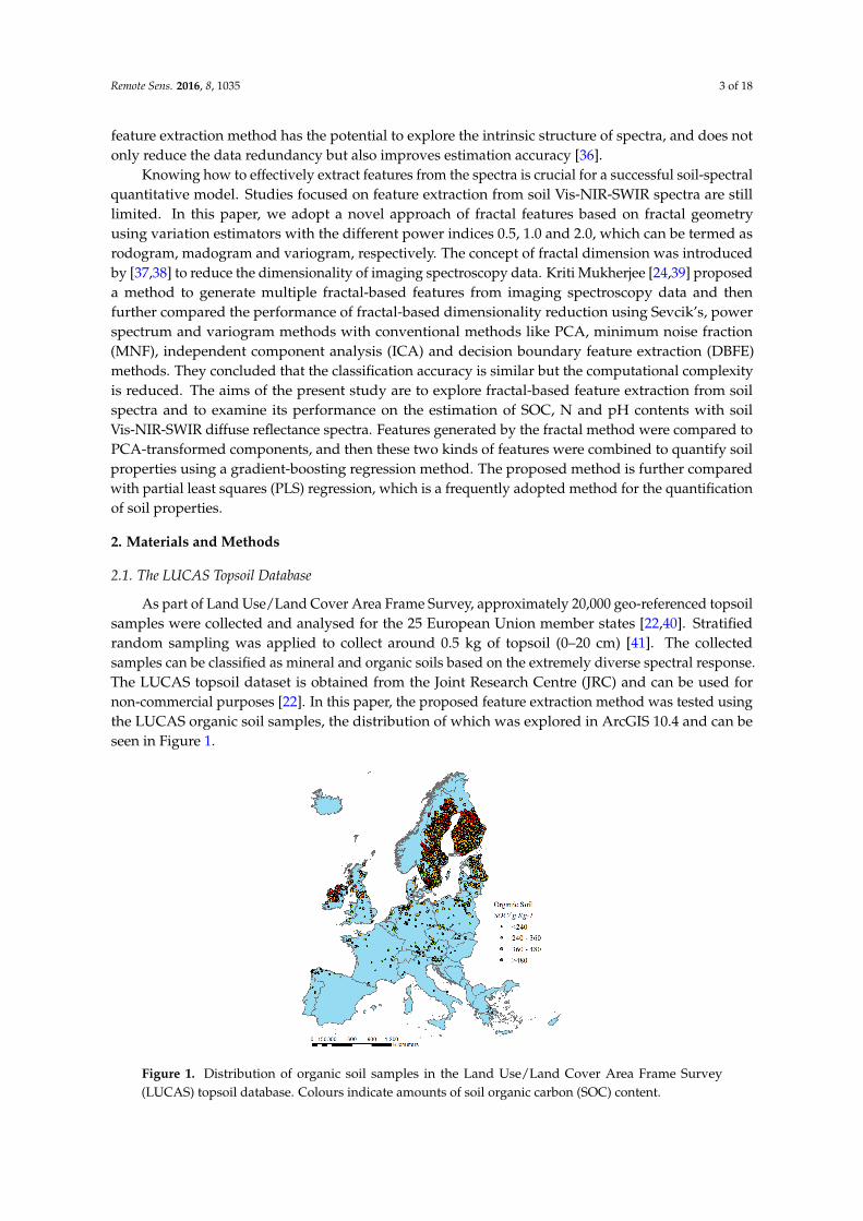
As part of Land Use/Land Cover Area Frame Survey, approximately 20,000 geo-referenced topsoilsamples were collected and analysed for the 25 European Union member states [22,40]. Stratifiedrandom sampling was applied to collect around 0.5 kg of topsoil (0–20 cm) [41]. The collectedsamples can be classified as mineral and organic soils based on the extremely diverse spectral response.The LUCAS topsoil dataset is obtained from the Joint Research Centre (JRC) and can be used fornon-commercial purposes [22]. In this paper, the proposed feature extraction method was tested usingthe LUCAS organic soil samples, the distribution of which was explored in ArcGIS 10.4 and can beseen in Figure 1.

Remote Sens. 2016, 8, 1035 3 of 19

Knowing how to effectively extract features from the spectra is crucial for a successful soil-spectral quantitative model. Studies focused on feature extraction from soil Vis-NIR-SWIR spectra are still limited. In this paper, we adopt a novel approach of fractal features based on fractal geometry using variation estimators with the different power indices 0.5, 1.0 and 2.0, which can be termed as rodogram, madogram and variogram, respectively. The concept of fractal dimension was introduced by [37,38] to reduce the dimensionality of imaging spectroscopy data. Kriti Mukherjee [24,39] proposed a method to generate multiple fractal-based features from imaging spectroscopy data and then further compared the performance of fractal-based dimensionality reduction using Sevcik’s, power spectrum and variogram methods with conventional methods like PCA, minimum noise fraction (MNF), independent component analysis (ICA) and decision boundary feature extraction (DBFE) methods. They concluded that the classification accuracy is similar but the computational complexity is reduced. The aims of the present study are to explore fractal-based feature extraction from soil spectra and to examine its performance on the estimation of SOC, N and pH contents with soil Vis-NIR-SWIR diffuse reflectance spectra. Features generated by the fractal method were compared to PCA-transformed components, and then these two kinds of features were combined to quantify soil properties using a gradient-boosting regression method. The proposed method is further compared with partial least squares (PLS) regression, which is a frequently adopted method for the quantification of soil properties.

2. Materials and Methods

2.1. The LUCAS Topsoil Database

As part of Land Use/Land Cover Area Frame Survey, approximately 20,000 geo-referenced topsoil samples were collected and analysed for the 25 European Union member states [22,40]. Stratified random sampling was applied to collect around 0.5 kg of topsoil (0–20 cm) [41]. The collected samples can be classified as mineral and organic soils based on the extremely diverse spectral response. The LUCAS topsoil dataset is obtained from the Joint Research Centre (JRC) and can be used for non-commercial purposes [22]. In this paper, the proposed feature extraction method was tested using the LUCAS organic soil samples, the distribution of which was explored in ArcGIS 10.4 and can be seen in Figure 1.

Figure 1. Distribution of organic soil samples in the Land Use/Land Cover Area Frame Survey (LUCAS) topsoil database. Colours indicate amounts of soil organic carbon (SOC) content.

Figure 1. Distribution of organic soil samples in the Land Use/Land Cover Area Frame Survey(LUCAS) topsoil database. Colours indicate amounts of soil organic carbon (SOC) content.

Remote Sens. 2016, 8, 1035 4 of 18

The Vis-NIR-SWIR soil spectra were measured using a FOSS XDS Rapid Content Analyser (FOSSNIRSystems Inc., Denmark) [22], operating in the 400–2500 nm wavelength range, with 0.5 nm spectralresolution. Organic soil spectra were pre-processed by removing the data at wavelengths of 400–500 nmthat showed instrumental artefacts, transformation of absorbance (A) spectra into reflectance (1/10A)spectra, continuum removal, Savitzky-Golay filter with a window size of 50, second order polynomialand first derivative. Thirteen soil properties have been analysed in a central laboratory [22], includingthe percentage of coarse fragments, particle size distribution (% clay, silt and sand content), pH (inCaCl2 and H2O), soil organic carbon (g/kg), carbonate content (g/kg), phosphorous content (mg/kg),total nitrogen content (g/kg), extractable potassium content (mg/kg), and cation exchange capacity(cmol(+)/kg). Three key soil fertility properties, soil organic carbon (SOC), total nitrogen content (N)and pH in CaCl2 (pH), were selected as our studied properties.

2.2. Fractal Feature Extraction Method

2.2.1. Concept of Fractal Dimension

Fractal dimension is a robust method for describing natural or man-made fractals having thefundamental feature known and referred to as self-similarity [42]. Within the fractal lies anothercopy of the same fractal, smaller but complete. If we have a strictly self-similar fractal which can bedecomposed into N pieces, each of which is a copy of the original fractal scaled by a factor of S, then,

SD = N (1)

where D is the Hausdorff Dimension. D is a non-integer number, describing how the irregular structureof objects and/or phenomena is replicated in an iterative way from small to large scales. Anything thatappears random and irregular can be a fractal, strictly or statistically, including the soil Vis-NIR-SWIRspectrum, which cannot be defined by any mathematical equation and is therefore considered asan irregular curve. There are numerous methods which have been developed for fractal dimensionestimation, including box-count [43], variogram [44], power spectrum [24] and spectral [45] methods.

2.2.2. Variation Method for Fractal Dimension

The variogram estimator is widely used in the determination of the fractal dimension and it isknown for its ease of use [46]. By sampling a large number of pairs of points along the spectral curveand computing the differences in their reflectance values, the fractal dimension is easily derived fromthe log–log plot of variogram and lags. Xu and Xt+u are two reflectance values located at points u andt+u, and these two points are separated by the lag of t. The variogram can be calculated as the meansum of squares of all differences between pairs of values with a given distance divided by two.

γ(t) =12

E(Xu − Xt+u)2 (2)

The variogram estimator is a stochastic process with stationary increments as half times theexpectation of the square of an increment at lag t, and a generalisation of the variation estimator can beobtained with different order p of a stochastic process [47]:

γp(t) =12

E|Xu − Xt+u|p (3)

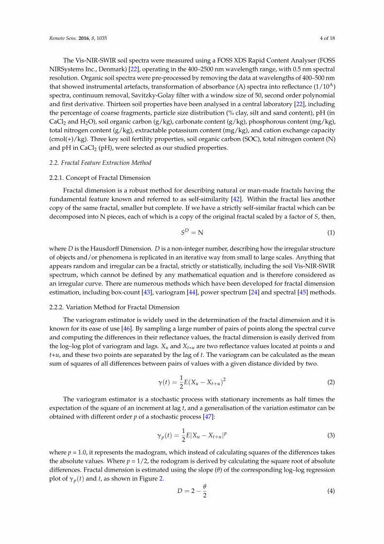
where p = 1.0, it represents the madogram, which instead of calculating squares of the differences takesthe absolute values. Where p = 1/2, the rodogram is derived by calculating the square root of absolutedifferences. Fractal dimension is estimated using the slope (θ) of the corresponding log–log regressionplot of γp(t) and t, as shown in Figure 2.

D = 2− θ

2(4)

Remote Sens. 2016, 8, 1035 5 of 18Remote Sens. 2016, 8, 1035 5 of 19

Figure 2. Illustration of fractal dimension calculation. (A) is the spectral curve and (B) is the corresponding log–log plot of variogram and lags and the fitted regression line.

2.2.3. Fractal Feature Generation

Fractal features are generated by multiplying spectral energy with the corresponding fractal dimension. As the fractal dimension can be calculated using the whole curve or only part of the curve, the spectrum can be segmented into several parts and each part corresponds to a new fractal feature. For a soil spectral curve, a common approach is to evenly divide the whole curve into a desired number of segments [48], which means the step and window size are the same. In this study, we explored the effect of different combinations of step and window sizes on generated fractal features. The final feature number Nf can be calculated as: = − 1 (5)

is the number of raw spectral measurements, is the value of step size and W is the value of moving window size. W is obtained by multiplying scale and step value. It should be pointed out that the scale here is not the scaling factor for fractal dimension. When the window size is equal to the scale size, the fractal dimension of the spectral segment is calculated using reflectance values within the same wavelength window. The window size is often defined as larger than the step size, which means segments of the same spectral curve are overlapping. Step size is defined as 100.0 nm and moving window size as 200.0 nm, as shown in Figure 3, which means = 200 and w = 400 (the spectral resolution is 0.5 nm in our case). New fractal features can be generated when the wavelength window moves along the spectral curve at step 100.0 nm. With the increase of the step size, the final fractal feature number (Nf) correspondingly decreases, which can be used as a means of dimension reduction.

For a certain scale value, s, Nf numbers of fractal dimension values can be obtained by moving along the spectral curve at step size p. For each segment, the number of points are marked as n and can be calculated by Equation (5). The reflectance value as Zj (j = 1, 2,…,n) and the corresponding fractal dimension value can be calculated according to Equation (4) as Dm (m = 1, 2,…,Nf), and fractal features at scale s by: = D E (6)

where E is the spectral energy and can be derived from the following equation:

E = , (7)

Figure 2. Illustration of fractal dimension calculation. (A) is the spectral curve and (B) is thecorresponding log–log plot of variogram and lags and the fitted regression line.

2.2.3. Fractal Feature Generation

Fractal features are generated by multiplying spectral energy with the corresponding fractaldimension. As the fractal dimension can be calculated using the whole curve or only part of the curve,the spectrum can be segmented into several parts and each part corresponds to a new fractal feature.For a soil spectral curve, a common approach is to evenly divide the whole curve into a desired numberof segments [48], which means the step and window size are the same. In this study, we exploredthe effect of different combinations of step and window sizes on generated fractal features. The finalfeature number Nf can be calculated as:

N f =Nr −W

P+ 1 (5)

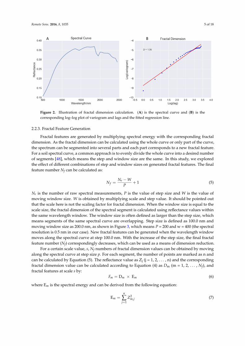
Nr is the number of raw spectral measurements, P is the value of step size and W is the value ofmoving window size. W is obtained by multiplying scale and step value. It should be pointed outthat the scale here is not the scaling factor for fractal dimension. When the window size is equal to thescale size, the fractal dimension of the spectral segment is calculated using reflectance values withinthe same wavelength window. The window size is often defined as larger than the step size, whichmeans segments of the same spectral curve are overlapping. Step size is defined as 100.0 nm andmoving window size as 200.0 nm, as shown in Figure 3, which means P = 200 and w = 400 (the spectralresolution is 0.5 nm in our case). New fractal features can be generated when the wavelength windowmoves along the spectral curve at step 100.0 nm. With the increase of the step size, the final fractalfeature number (Nf) correspondingly decreases, which can be used as a means of dimension reduction.

For a certain scale value, s, Nf numbers of fractal dimension values can be obtained by movingalong the spectral curve at step size p. For each segment, the number of points are marked as n andcan be calculated by Equation (5). The reflectance value as Zj (j = 1, 2, . . . , n) and the correspondingfractal dimension value can be calculated according to Equation (4) as Dm (m = 1, 2, . . . , Nf), andfractal features at scale s by:

Fm = Dm × Em (6)

where Em is the spectral energy and can be derived from the following equation:

Em =n

∑j=1

Z2m,j (7)

Remote Sens. 2016, 8, 1035 6 of 18

Remote Sens. 2016, 8, 1035 6 of 19

Figure 3. Illustration of the meaning of step and window size for multiple fractal feature generation. (step size = 100.0 nm, window size = 200.0 nm).

2.3. Gradient-Boosting Regression Model

Soil spectroscopy quantitatively correlates with soil properties, which supposes that fitting a regression model with features extracted from spectra will have good predictive accuracies with respect to soil continuous properties. Gradient-boosting is a highly effective and widely used machine-learning approach [49]. Gradient-boosting develops an ensemble of tree-based models by training each of the trees in the ensemble on different labels and then combining the trees. It can produce robust and interpretable procedures for both regression and classification. For a regression problem where the objective is to maximize the coefficient of determination (R2) or to minimize the root mean square error (RMSE), each successive tree is trained on the errors left over by the collection of earlier trees. XGBoost is a scalable and flexible gradient-boosting library [50–52], which is adopted to build the soil spectral quantitative model in our study. XGBoost uses more regularised model formalisation to control over-fitting, which gives it better performance. Mathematically, the model can be viewed as:

= ( ), ∈ (8)

where is the number of trees, f is a function in the functional space , and is the set of all possible regression trees. Therefore, the objective of optimization can be written as:

( ) = ( , ) Ω( ) (9)

where ( , ) is the training loss function, and Ω( ) is the regularization term. The goal of XGBoost model is to minimize ( ). 2.4. Evaluation

For each soil property, the soil spectral quantitative model was developed on a random sample of two-thirds of the selected soil samples using the gradient-boosting regression method. The calibrations were tested by predicting the soil properties on validation data sets composed of the remaining one-third of the organic soil samples. No samples were omitted from the analysis, nor the calibration or validation data sets. The model accuracies were evaluated on estimated and measured soil SOC, N and pH values using RMSE, R2 and the ratio of percent deviation (RPD). = ∑ ( − )∑ ( − ) (10)

Figure 3. Illustration of the meaning of step and window size for multiple fractal feature generation.(step size = 100.0 nm, window size = 200.0 nm).

2.3. Gradient-Boosting Regression Model

Soil spectroscopy quantitatively correlates with soil properties, which supposes that fitting aregression model with features extracted from spectra will have good predictive accuracies with respectto soil continuous properties. Gradient-boosting is a highly effective and widely used machine-learningapproach [49]. Gradient-boosting develops an ensemble of tree-based models by training each of thetrees in the ensemble on different labels and then combining the trees. It can produce robust andinterpretable procedures for both regression and classification. For a regression problem where theobjective is to maximize the coefficient of determination (R2) or to minimize the root mean squareerror (RMSE), each successive tree is trained on the errors left over by the collection of earlier trees.XGBoost is a scalable and flexible gradient-boosting library [50–52], which is adopted to build thesoil spectral quantitative model in our study. XGBoost uses more regularised model formalisation tocontrol over-fitting, which gives it better performance. Mathematically, the model can be viewed as:

yi =K

∑k=1

fk(xi), fk ∈ F (8)

where K is the number of trees, f is a function in the functional space F, and F is the set of all possibleregression trees. Therefore, the objective of optimization can be written as:

obj(θ) =n

∑i

l(yi, yi) +K

∑k=1

Ω( fk) (9)

where l(yi, yi) is the training loss function, and Ω( fk) is the regularization term. The goal of XGBoostmodel is to minimize obj(θ).

2.4. Evaluation

For each soil property, the soil spectral quantitative model was developed on a random sample oftwo-thirds of the selected soil samples using the gradient-boosting regression method. The calibrationswere tested by predicting the soil properties on validation data sets composed of the remainingone-third of the organic soil samples. No samples were omitted from the analysis, nor the calibrationor validation data sets. The model accuracies were evaluated on estimated and measured soil SOC,N and pH values using RMSE, R2 and the ratio of percent deviation (RPD).

Remote Sens. 2016, 8, 1035 7 of 18

R2 =∑n

i=1(yi − y)2

∑ni=1(Yi −Y

)2 (10)

RMSE =

√1n ∑ n

i=1(yi − yi)2 (11)

RPD =SD

RMSE(12)

where n is the number of validation samples, y is the measured values, y is the mean of the measuredvalues, and y is the estimated values. RPD is the ratio of the standard deviation (SD) of the calibrationdata to the RMSE of the validation data [53]. An RPD <1.0 indicates a very poor model and its useis not recommended; an RPD between 1.0 and 1.4 indicates a poor model where only high and lowvalues are distinguishable; an RPD between 1.4 and 1.8 indicates a fair model which may be used forassessment and correlation; RPD values between 1.8 and 2.0 indicate a good model where quantitativepredictions are possible; an RPD between 2.0 and 2.5 indicates a very good, quantitative model, and anRPD >2.5 indicates an excellent model.

3. Results

3.1. Fractal Features for Soil Spectroscopy

For a single soil Vis-NIR-SWIR spectrum, the fractal dimension can be calculated by Equation (4).Before extracting fractal features from soil spectra, we first examined the relationship between soilproperties and the corresponding fractal dimension. Spectral values of soil are relatively low andthe curve appears smoother compared with other objects like vegetation. Thus, the resulting fractaldimension values are comparatively low. Since the fractal dimension is derived from the slope ofthe regression line obtained from the log–log plot of γp(t) and lag t, one problem is how many lagincrements are necessary to produce reliable results. Theoretically only a minimum of two points isnecessary to make such a plot [46]. However, the results of such an analysis tend to not be reliable orrepresentative. In this study, the value of lag increments was set as 5, and the Pearson correlations ofsoil properties and fractal dimensions are shown in Table 1. The Pearson is a standardized covarianceand ranges from −1 to +1, which indicates a perfect negative (−1) or positive (+1) linear relationshiprespectively. A value of zero is not related to the independency between the two variables, it onlysuggests no linear association. It can be seen that SOC, N and pH have negative relationships withfractal dimension. SOC and N have similar correlations with fractal dimension. Among these threeestimators, the variogram-based fractal dimension calculation method achieved the best correlationbetween fractal dimension values and soil properties SOC (correlation coefficient (r) = −0.54), N(r = −0.50) and pH (r = −0.12).

Table 1. Pearson correlation coefficients between soil properties and fractal dimensions calculated byrodogram, madogram and variogram estimators.

Rodogram Madogram Variogram

SOC −0.40 −0.47 −0.54N −0.38 −0.43 −0.50

pH −0.12 −0.13 −0.12

An intact spectrum can be divided into multiple segments, overlapping or non-overlapping. Eachsegment is corresponding to a fractal feature. When step size and window size are respectively set to2.5 nm and 50.0 nm, a total number of 791 fractal features can be derived by rodogram, madogram orvariogram methods, resulting the original spectral dimension reduced from 4000 to 791. In order tomake a proper comparison between the generated fractal feature-based curve and the raw spectral

Remote Sens. 2016, 8, 1035 8 of 18

curve, the centre wavelength value of the spectral segment is assigned to the fractal feature as thecorresponding “wavelength number”.

A great advantage of fractal-based feature extraction is that the curve shape of fractal featuresis similar to the shape of raw spectrum, which makes it possible to apply methods like continuumremoval (CR) not only to the raw spectrum but also to the fractal-based “spectrum”. The organic soilsamples can be divided into four groups according to the content of SOC. Average spectral reflectanceand continuum removal reflectance of LUCAS organic soil samples were computed by SOC classes(Figure 4A). For fractal features, average fractal energy and continuum removal responses of organicsoil samples were also computed and shown in Figure 4B–D. The highest SOC class that was above480 g/kg showed the highest mean reflectance in wavelength range from 1000.0 nm to 2000.0 nm,which is consistent with observations in the literature [4]. The continuum removal reflectance showeda strong correlation with SOC content at a wavelength of near 600.0 nm. The difference between rawspectral curve and fractal feature curve was not obvious from the view of shape. Fractal featuresshowed shallow absorption peak in proportion for SOC classes at a wavelength of 600.0 nm. The fractalenergy values were larger than reflectance values, as the former were multiplied by spectral energyand fractal dimension, which was supposed to be larger than 1.0.

Remote Sens. 2016, 8, 1035 8 of 19

removal (CR) not only to the raw spectrum but also to the fractal-based “spectrum”. The organic soil samples can be divided into four groups according to the content of SOC. Average spectral reflectance and continuum removal reflectance of LUCAS organic soil samples were computed by SOC classes (Figure 4A). For fractal features, average fractal energy and continuum removal responses of organic soil samples were also computed and shown in Figure 4B–D. The highest SOC class that was above 480 g/kg showed the highest mean reflectance in wavelength range from 1000.0 nm to 2000.0 nm, which is consistent with observations in the literature [4]. The continuum removal reflectance showed a strong correlation with SOC content at a wavelength of near 600.0 nm. The difference between raw spectral curve and fractal feature curve was not obvious from the view of shape. Fractal features showed shallow absorption peak in proportion for SOC classes at a wavelength of 600.0 nm. The fractal energy values were larger than reflectance values, as the former were multiplied by spectral energy and fractal dimension, which was supposed to be larger than 1.0.

Figure 4. (A) Average spectral reflectance and continuum removal reflectance of LUCAS organic soil samples computed by SOC classes. (B–D) Average fractal energy and continuum removal responses of organic soil samples computed by SOC classes using rodogram, madogram and variogram estimators respectively. The central wavelength number of the corresponding spectral segment is assigned to the fractal feature.

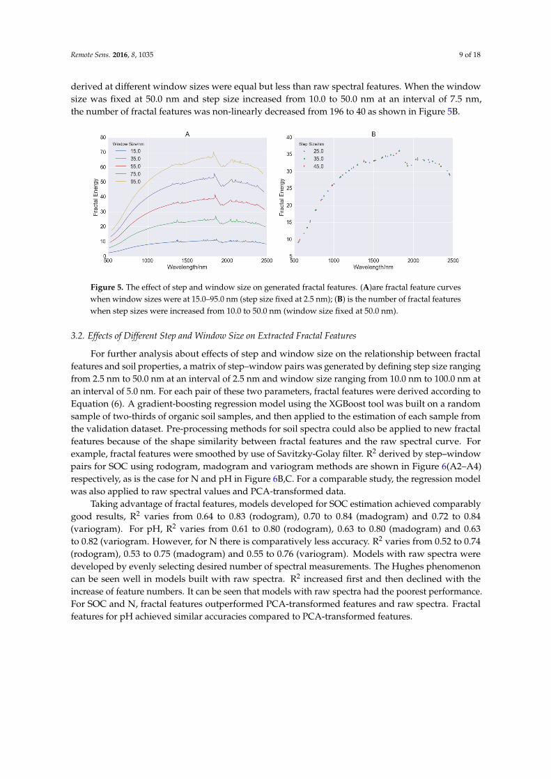
To demonstrate the effects of step and window size on extracted fractal features, the combinations of the two parameters were tested. When the step size was fixed at 2.5 nm, a series of fractal feature curves were derived by defining window sizes as 15.0 nm, 35.0 nm, 55.0 nm, 75.0 nm and 95.0 nm. With the increase of window size, fractal energies correspondingly increased and the shapes of fractal features were also gradually exaggerated, as shown in Figure 5A. The number for fractal features derived at different window sizes were equal but less than raw spectral features. When the window size was fixed at 50.0 nm and step size increased from 10.0 to 50.0 nm at an interval of 7.5 nm, the number of fractal features was non-linearly decreased from 196 to 40 as shown in Figure 5B.

Figure 4. (A) Average spectral reflectance and continuum removal reflectance of LUCAS organic soilsamples computed by SOC classes. (B–D) Average fractal energy and continuum removal responses oforganic soil samples computed by SOC classes using rodogram, madogram and variogram estimatorsrespectively. The central wavelength number of the corresponding spectral segment is assigned to thefractal feature.

To demonstrate the effects of step and window size on extracted fractal features, the combinationsof the two parameters were tested. When the step size was fixed at 2.5 nm, a series of fractal featurecurves were derived by defining window sizes as 15.0 nm, 35.0 nm, 55.0 nm, 75.0 nm and 95.0 nm.With the increase of window size, fractal energies correspondingly increased and the shapes of fractalfeatures were also gradually exaggerated, as shown in Figure 5A. The number for fractal features

Remote Sens. 2016, 8, 1035 9 of 18

derived at different window sizes were equal but less than raw spectral features. When the windowsize was fixed at 50.0 nm and step size increased from 10.0 to 50.0 nm at an interval of 7.5 nm,the number of fractal features was non-linearly decreased from 196 to 40 as shown in Figure 5B.Remote Sens. 2016, 8, 1035 9 of 19

Figure 5. The effect of step and window size on generated fractal features. (A )are fractal feature curves when window sizes were at 15.0–95.0 nm (step size fixed at 2.5 nm); (B) is the number of fractal features when step sizes were increased from 10.0 to 50.0 nm (window size fixed at 50.0 nm).

3.2. Effects of Different Step and Window Size on Extracted Fractal Features

For further analysis about effects of step and window size on the relationship between fractal features and soil properties, a matrix of step–window pairs was generated by defining step size ranging from 2.5 nm to 50.0 nm at an interval of 2.5 nm and window size ranging from 10.0 nm to 100.0 nm at an interval of 5.0 nm. For each pair of these two parameters, fractal features were derived according to Equation (6). A gradient-boosting regression model using the XGBoost tool was built on a random sample of two-thirds of organic soil samples, and then applied to the estimation of each sample from the validation dataset. Pre-processing methods for soil spectra could also be applied to new fractal features because of the shape similarity between fractal features and the raw spectral curve. For example, fractal features were smoothed by use of Savitzky-Golay filter. R2 derived by step–window pairs for SOC using rodogram, madogram and variogram methods are shown in Figure 6(A2–A4) respectively, as is the case for N and pH in Figure 6B,C. For a comparable study, the regression model was also applied to raw spectral values and PCA-transformed data.

Taking advantage of fractal features, models developed for SOC estimation achieved comparably good results, R2 varies from 0.64 to 0.83 (rodogram), 0.70 to 0.84 (madogram) and 0.72 to 0.84 (variogram). For pH, R2 varies from 0.61 to 0.80 (rodogram), 0.63 to 0.80 (madogram) and 0.63 to 0.82 (variogram. However, for N there is comparatively less accuracy. R2 varies from 0.52 to 0.74 (rodogram), 0.53 to 0.75 (madogram) and 0.55 to 0.76 (variogram). Models with raw spectra were developed by evenly selecting desired number of spectral measurements. The Hughes phenomenon can be seen well in models built with raw spectra. R2 increased first and then declined with the increase of feature numbers. It can be seen that models with raw spectra had the poorest performance. For SOC and N, fractal features outperformed PCA-transformed features and raw spectra. Fractal features for pH achieved similar accuracies compared to PCA-transformed features.

Figure 5. The effect of step and window size on generated fractal features. (A)are fractal feature curveswhen window sizes were at 15.0–95.0 nm (step size fixed at 2.5 nm); (B) is the number of fractal featureswhen step sizes were increased from 10.0 to 50.0 nm (window size fixed at 50.0 nm).

3.2. Effects of Different Step and Window Size on Extracted Fractal Features

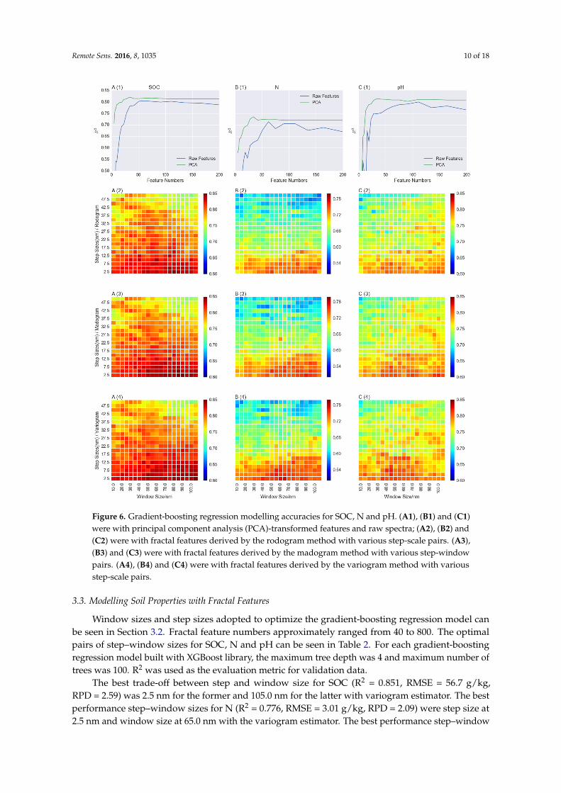
For further analysis about effects of step and window size on the relationship between fractalfeatures and soil properties, a matrix of step–window pairs was generated by defining step size rangingfrom 2.5 nm to 50.0 nm at an interval of 2.5 nm and window size ranging from 10.0 nm to 100.0 nm atan interval of 5.0 nm. For each pair of these two parameters, fractal features were derived according toEquation (6). A gradient-boosting regression model using the XGBoost tool was built on a randomsample of two-thirds of organic soil samples, and then applied to the estimation of each sample fromthe validation dataset. Pre-processing methods for soil spectra could also be applied to new fractalfeatures because of the shape similarity between fractal features and the raw spectral curve. Forexample, fractal features were smoothed by use of Savitzky-Golay filter. R2 derived by step–windowpairs for SOC using rodogram, madogram and variogram methods are shown in Figure 6(A2–A4)respectively, as is the case for N and pH in Figure 6B,C. For a comparable study, the regression modelwas also applied to raw spectral values and PCA-transformed data.

Taking advantage of fractal features, models developed for SOC estimation achieved comparablygood results, R2 varies from 0.64 to 0.83 (rodogram), 0.70 to 0.84 (madogram) and 0.72 to 0.84(variogram). For pH, R2 varies from 0.61 to 0.80 (rodogram), 0.63 to 0.80 (madogram) and 0.63to 0.82 (variogram. However, for N there is comparatively less accuracy. R2 varies from 0.52 to 0.74(rodogram), 0.53 to 0.75 (madogram) and 0.55 to 0.76 (variogram). Models with raw spectra weredeveloped by evenly selecting desired number of spectral measurements. The Hughes phenomenoncan be seen well in models built with raw spectra. R2 increased first and then declined with theincrease of feature numbers. It can be seen that models with raw spectra had the poorest performance.For SOC and N, fractal features outperformed PCA-transformed features and raw spectra. Fractalfeatures for pH achieved similar accuracies compared to PCA-transformed features.

Remote Sens. 2016, 8, 1035 10 of 18

Remote Sens. 2016, 8, 1035 10 of 19

Figure 6. Gradient-boosting regression modelling accuracies for SOC, N and pH. (A1), (B1) and (C1) were with principal component analysis (PCA)-transformed features and raw spectra; (A2), (B2) and (C2) were with fractal features derived by the rodogram method with various step-scale pairs. (A3), (B3) and (C3) were with fractal features derived by the madogram method with various step-window pairs. (A4), (B4) and (C4) were with fractal features derived by the variogram method with various step-scale pairs.

3.3. Modelling Soil Properties with Fractal Features

Window sizes and step sizes adopted to optimize the gradient-boosting regression model can be seen in Section 3.2. Fractal feature numbers approximately ranged from 40 to 800. The optimal pairs of step–window sizes for SOC, N and pH can be seen in Table 2. For each gradient-boosting regression model built with XGBoost library, the maximum tree depth was 4 and maximum number of trees was 100. R2 was used as the evaluation metric for validation data.

The best trade-off between step and window size for SOC (R2 = 0.851, RMSE = 56.7 g/kg, RPD = 2.59) was 2.5 nm for the former and 105.0 nm for the latter with variogram estimator. The best performance step–window sizes for N (R2 = 0.776, RMSE = 3.01 g/kg, RPD = 2.09) were step size at 2.5 nm and window size at 65.0 nm with the variogram estimator. The best performance step–window size for N (R2 = 0.822, RMSE = 0.49, RPD = 2.31) were step size at 7.5 nm and window size at 45.0 nm with the variogram estimator. From Table 2, it can be seen that fractal-based feature extraction methods tend

Figure 6. Gradient-boosting regression modelling accuracies for SOC, N and pH. (A1), (B1) and (C1)were with principal component analysis (PCA)-transformed features and raw spectra; (A2), (B2) and(C2) were with fractal features derived by the rodogram method with various step-scale pairs. (A3),(B3) and (C3) were with fractal features derived by the madogram method with various step-windowpairs. (A4), (B4) and (C4) were with fractal features derived by the variogram method with variousstep-scale pairs.

3.3. Modelling Soil Properties with Fractal Features

Window sizes and step sizes adopted to optimize the gradient-boosting regression model canbe seen in Section 3.2. Fractal feature numbers approximately ranged from 40 to 800. The optimalpairs of step–window sizes for SOC, N and pH can be seen in Table 2. For each gradient-boostingregression model built with XGBoost library, the maximum tree depth was 4 and maximum number oftrees was 100. R2 was used as the evaluation metric for validation data.

The best trade-off between step and window size for SOC (R2 = 0.851, RMSE = 56.7 g/kg,RPD = 2.59) was 2.5 nm for the former and 105.0 nm for the latter with variogram estimator. The bestperformance step–window sizes for N (R2 = 0.776, RMSE = 3.01 g/kg, RPD = 2.09) were step size at2.5 nm and window size at 65.0 nm with the variogram estimator. The best performance step–window

Remote Sens. 2016, 8, 1035 11 of 18

size for N (R2 = 0.822, RMSE = 0.49, RPD = 2.31) were step size at 7.5 nm and window size at 45.0 nmwith the variogram estimator. From Table 2, it can be seen that fractal-based feature extraction methodstend to keep a much larger number of features compared to PCA. To achieve similar performanceof PCA, fractal-based approaches need to retain ~200 features, such as 190 for SOC (R2 = 0.819,RMSE = 62.49 g/kg, RPD = 2.34) where step size and window size were respectively 10.0 nm and105.0 nm, 128 features for N (R2 = 0.736, RMSE = 3.26 g/kg, RPD = 1.92) where step size and windowsize were respectively 15.0 nm and 135.0 nm, and 131 features for pH (R2 = 0.807, RMSE = 0.50,RPD = 2.22) where step size and window size were respectively 15.0 nm and 50.0 nm.

In real-world examples, there are many ways to extract features from a dataset. Often it isbeneficial to combine several methods to obtain good performance. To assess whether predictiveaccuracy could be enhanced by integrating multiple features, the first 30 PCA components werecombined with fractal features and then ingested into the gradient-boosting regression model.Combined features showed better performance when applied for the estimation of all three soilproperties, SOC (R2 = 0.86, RMSE = 55.16 g/kg, RPD = 2.7), N (R2 = 0.78, RMSE = 2.96 g/kg, RPD = 2.19)and pH (R2 = 0.85, RMSE = 0.44, RPD = 2.59), as shown in Figure 7.

Remote Sens. 2016, 8, 1035 11 of 19

to keep a much larger number of features compared to PCA. To achieve similar performance of PCA, fractal-based approaches need to retain ~200 features, such as 190 for SOC (R2 = 0.819, RMSE = 62.49 g/kg, RPD = 2.34) where step size and window size were respectively 10.0 nm and 105.0 nm, 128 features for N (R2 = 0.736, RMSE = 3.26 g/kg, RPD = 1.92) where step size and window size were respectively 15.0 nm and 135.0 nm, and 131 features for pH (R2 = 0.807, RMSE = 0.50, RPD = 2.22) where step size and window size were respectively 15.0 nm and 50.0 nm.

In real-world examples, there are many ways to extract features from a dataset. Often it is beneficial to combine several methods to obtain good performance. To assess whether predictive accuracy could be enhanced by integrating multiple features, the first 30 PCA components were combined with fractal features and then ingested into the gradient-boosting regression model. Combined features showed better performance when applied for the estimation of all three soil properties, SOC (R2 = 0.86, RMSE = 55.16 g/kg, RPD = 2.7), N (R2 = 0.78, RMSE = 2.96 g/kg, RPD = 2.19) and pH (R2 = 0.85, RMSE = 0.44, RPD = 2.59), as shown in Figure 7.

Figure 7. Best performance of gradient-boosting regression modelling accuracies for SOC, N and pH. (A1), (A2) and (A3) were with PCA-transformed features. (B1), (B2) and (B3) were with fractal features. (C1), (C2) and (C3) were with features combined by PCA-transformed features and fractal features. R2: coefficient of determination; RMSE: root mean square error; RPD: the ratio of percent deviation.

Figure 7. Best performance of gradient-boosting regression modelling accuracies for SOC, N and pH.(A1), (A2) and (A3) were with PCA-transformed features. (B1), (B2) and (B3) were with fractal features.(C1), (C2) and (C3) were with features combined by PCA-transformed features and fractal features.R2: coefficient of determination; RMSE: root mean square error; RPD: the ratio of percent deviation.

Remote Sens. 2016, 8, 1035 12 of 18

Table 2. Best Performance step–window pairs for soil properties estimation using fractal-based featureextraction and comparison with PCA. R2: coefficient of determination.

Method Step Size/nm Window Size/nm Dimension R2

SOC

PCA - - 28 0.813Rodogram 2.5 80 769 0.847Madogram 2.5 90 765 0.847Variogram 2.5 105 759 0.851

N

PCA - - 34 0.735Rodogram 2.5 50 781 0.756Madogram 2.5 90 765 0.767Variogram 2.5 65 775 0.776

pH

PCA - - 34 0.814Rodogram 5 55 390 0.806Madogram 2.5 100 761 0.818Variogram 7.5 45 261 0.821

3.4. Comparison with PLS Regression

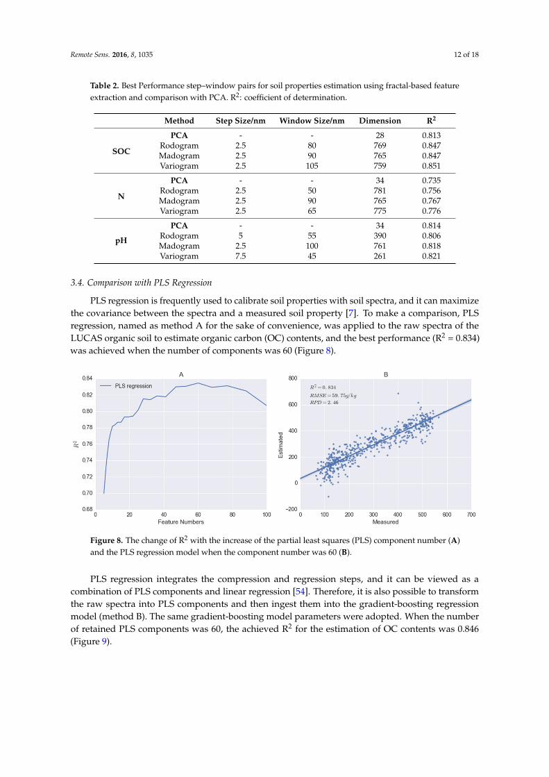
PLS regression is frequently used to calibrate soil properties with soil spectra, and it can maximizethe covariance between the spectra and a measured soil property [7]. To make a comparison, PLSregression, named as method A for the sake of convenience, was applied to the raw spectra of theLUCAS organic soil to estimate organic carbon (OC) contents, and the best performance (R2 = 0.834)was achieved when the number of components was 60 (Figure 8).

Remote Sens. 2016, 8, 1035 12 of 19

Table 2. Best Performance step–window pairs for soil properties estimation using fractal-based feature extraction and comparison with PCA. R2: coefficient of determination.

Method Step Size/nm Window Size/nm Dimension R2

SOC

PCA - - 28 0.813 Rodogram 2.5 80 769 0.847 Madogram 2.5 90 765 0.847 Variogram 2.5 105 759 0.851

N

PCA - - 34 0.735 Rodogram 2.5 50 781 0.756 Madogram 2.5 90 765 0.767 Variogram 2.5 65 775 0.776

pH

PCA - - 34 0.814 Rodogram 5 55 390 0.806 Madogram 2.5 100 761 0.818 Variogram 7.5 45 261 0.821

3.4. Comparison with PLS Regression

PLS regression is frequently used to calibrate soil properties with soil spectra, and it can maximize the covariance between the spectra and a measured soil property [7]. To make a comparison, PLS regression, named as method A for the sake of convenience, was applied to the raw spectra of the LUCAS organic soil to estimate organic carbon (OC) contents, and the best performance (R2 = 0.834 ) was achieved when the number of components was 60 (Figure 8).

Figure 8. The change of R2 with the increase of the partial least squares (PLS) component number (A) and the PLS regression model when the component number was 60 (B).

PLS regression integrates the compression and regression steps, and it can be viewed as a combination of PLS components and linear regression [54]. Therefore, it is also possible to transform the raw spectra into PLS components and then ingest them into the gradient-boosting regression model (method B). The same gradient-boosting model parameters were adopted. When the number of retained PLS components was 60, the achieved R2 for the estimation of OC contents was 0.846 (Figure 9).

Figure 8. The change of R2 with the increase of the partial least squares (PLS) component number (A)and the PLS regression model when the component number was 60 (B).

PLS regression integrates the compression and regression steps, and it can be viewed as acombination of PLS components and linear regression [54]. Therefore, it is also possible to transformthe raw spectra into PLS components and then ingest them into the gradient-boosting regressionmodel (method B). The same gradient-boosting model parameters were adopted. When the numberof retained PLS components was 60, the achieved R2 for the estimation of OC contents was 0.846(Figure 9).

Remote Sens. 2016, 8, 1035 13 of 18Remote Sens. 2016, 8, 1035 13 of 19

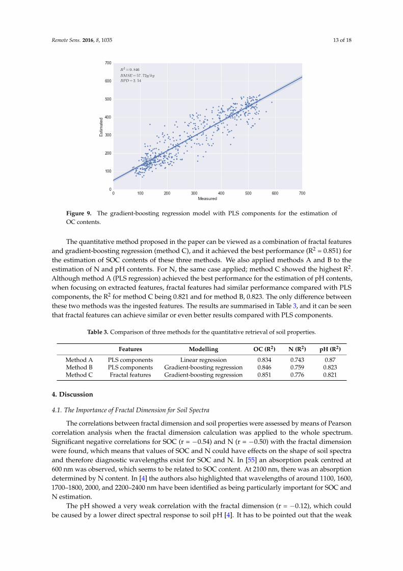
Figure 9. The gradient-boosting regression model with PLS components for the estimation of OC contents.

The quantitative method proposed in the paper can be viewed as a combination of fractal features and gradient-boosting regression (method C), and it achieved the best performance (R2 = 0.851) for the estimation of SOC contents of these three methods. We also applied methods A and B to the estimation of N and pH contents. For N, the same case applied; method C showed the highest R2. Although method A (PLS regression) achieved the best performance for the estimation of pH contents, when focusing on extracted features, fractal features had similar performance compared with PLS components, the R2 for method C being 0.821 and for method B, 0.823. The only difference between these two methods was the ingested features. The results are summarised in Table 3, and it can be seen that fractal features can achieve similar or even better results compared with PLS components.

Table 3. Comparison of three methods for the quantitative retrieval of soil properties.

Features Modelling OC (R2) N (R2) pH (R2)Method A PLS components Linear regression 0.834 0.743 0.87 Method B PLS components Gradient-boosting regression 0.846 0.759 0.823 Method C Fractal features Gradient-boosting regression 0.851 0.776 0.821

4. Discussion

4.1. The Importance of Fractal Dimension for Soil Spectra

The correlations between fractal dimension and soil properties were assessed by means of Pearson correlation analysis when the fractal dimension calculation was applied to the whole spectrum. Significant negative correlations for SOC (r = −0.54) and N (r = −0.50) with the fractal dimension were found, which means that values of SOC and N could have effects on the shape of soil spectra and therefore diagnostic wavelengths exist for SOC and N. In [55] an absorption peak centred at 600 nm was observed, which seems to be related to SOC content. At 2100 nm, there was an absorption determined by N content. In [4] the authors also highlighted that wavelengths of around 1100, 1600, 1700–1800, 2000, and 2200–2400 nm have been identified as being particularly important for SOC and N estimation.

The pH showed a very weak correlation with the fractal dimension (r = −0.12), which could be caused by a lower direct spectral response to soil pH [4]. It has to be pointed out that the weak correlation between pH and fractal dimension does not mean that soil spectra cannot be used to quantify soil pH values, but means that the variation of soil pH values does not significantly

Figure 9. The gradient-boosting regression model with PLS components for the estimation ofOC contents.

The quantitative method proposed in the paper can be viewed as a combination of fractal featuresand gradient-boosting regression (method C), and it achieved the best performance (R2 = 0.851) forthe estimation of SOC contents of these three methods. We also applied methods A and B to theestimation of N and pH contents. For N, the same case applied; method C showed the highest R2.Although method A (PLS regression) achieved the best performance for the estimation of pH contents,when focusing on extracted features, fractal features had similar performance compared with PLScomponents, the R2 for method C being 0.821 and for method B, 0.823. The only difference betweenthese two methods was the ingested features. The results are summarised in Table 3, and it can be seenthat fractal features can achieve similar or even better results compared with PLS components.

Table 3. Comparison of three methods for the quantitative retrieval of soil properties.

Features Modelling OC (R2) N (R2) pH (R2)

Method A PLS components Linear regression 0.834 0.743 0.87Method B PLS components Gradient-boosting regression 0.846 0.759 0.823Method C Fractal features Gradient-boosting regression 0.851 0.776 0.821

4. Discussion

4.1. The Importance of Fractal Dimension for Soil Spectra

The correlations between fractal dimension and soil properties were assessed by means of Pearsoncorrelation analysis when the fractal dimension calculation was applied to the whole spectrum.Significant negative correlations for SOC (r = −0.54) and N (r = −0.50) with the fractal dimensionwere found, which means that values of SOC and N could have effects on the shape of soil spectraand therefore diagnostic wavelengths exist for SOC and N. In [55] an absorption peak centred at600 nm was observed, which seems to be related to SOC content. At 2100 nm, there was an absorptiondetermined by N content. In [4] the authors also highlighted that wavelengths of around 1100, 1600,1700–1800, 2000, and 2200–2400 nm have been identified as being particularly important for SOC andN estimation.

The pH showed a very weak correlation with the fractal dimension (r = −0.12), which couldbe caused by a lower direct spectral response to soil pH [4]. It has to be pointed out that the weak

Remote Sens. 2016, 8, 1035 14 of 18

correlation between pH and fractal dimension does not mean that soil spectra cannot be used toquantify soil pH values, but means that the variation of soil pH values does not significantly contributeto the smoothness or roughness of the spectral curve. Soil pH value can still be well estimated in thelaboratory or in the field [55,56] using raw spectral data, which might be due to the mutual effect ofspectrally active soil constituents such as organic matter and clay [57]. It also can be seen that thePearson correlation between fractal dimension and soil properties has a positive relationship with theperformance of fractal features.

4.2. Modelling Soil Properties with Fractal Features

Three methods for the fractal dimension calculation and further feature extraction were studied inthis paper. The results demonstrate that the variogram estimator had slightly better performance thanthe madogram estimator when applied to fractal feature generation for soil property estimation, andmethods using these two estimators achieved better R2 than the method using the rodogram estimator.In [58] the classification achieved better results with texture layers derived from the madogram. Sincethe madogram estimator calculates the sum of the absolute value of the semivariance for all observedlags, it yields a softer effect on the presence of outliers compared to the variogram estimator. However,in our study, soil spectra were well pre-processed by the Savitzky–Golay filter and generated fractalfeatures. Fractal features generated by these three estimators have a similar curve shape and achievedvery close estimation accuracies for tested soil properties.

Step–window pairs have significant impact on estimation accuracies of soil properties. When thewindow size is fixed, accuracies are decreased with the increase of step size. However, when the stepsize is fixed, accuracies are prone to ascend slightly and then clearly descend. A higher R2 was foundto be located at the bottom of the step–window matrix. However, there is no guarantee as to whichstep–window pair is the best parameter for soil property estimation. Therefore, a hyper-parameteroptimisation method should be adopted for each of the soil properties.

In general, fractal features achieved better results compared to PCA-transformed features and rawspectra. This demonstrates that by taking advantage of fractal information encoded in the soil spectralshape, soil properties can be estimated in a better way. Besides, when raw data are transformed orprojected via PCA, measurement units and shape are lost. However, fractal-based feature extraction isprone to retaining much larger number of features compared to PCA. To achieve similar performance,the fractal-based approach needs ~200 feature numbers while PCA only needs ~30. When comparedwith PLS components, fractal features also had better performance for the estimation of OC and Ncontents. However, there is no conflict between common feature extraction practices with the proposedfractal method. When integrating different kinds of features, like PCA-transformed features and fractalfeatures, the performance is expected to be improved for the retrieval of soil properties.

5. Conclusions

Data acquisition with Vis-NIR-SWIR spectroscopy is relatively easy, and a wide range of soilproperties can be analysed within a comparatively short time with relatively little effort for samplepreparation. Soil spectroscopy has recently been identified as a method that has the potential to rapidlyestimate soil properties. Many soil-spectral libraries are already built at regional, continental or evenglobal scales. Various multivariate statistics methods have been successfully adopted to explore therelationship between soil spectra and soil physical/chemical properties. However, few studies arefocused on feature extraction from measured soil spectra, which is also crucial to correlating spectrawith soil properties.

The present study presents a novel methodology for feature extraction based on fractal geometry.Each Vis-NIR-SWIR spectrum can be divided into multiple segments by defining the moving windowsize and the step size. For each segmented spectral curve, the fractal dimension value was calculatedusing variation estimators. Fractal features, generated by multiplying the fractal dimension value withspectral energy, were further combined with PCA-transformed features, and the gradient-boosting

Remote Sens. 2016, 8, 1035 15 of 18

regression model achieved good performance with respect to the retrieval of SOC (R2 = 0.86,RMSE = 55.16 g/kg, RPD = 2.7), N (R2 = 0.78, RMSE = 2.96 g/kg, RPD = 2.19) and pH (R2 = 0.85,RMSE = 0.44, RPD = 2.59). Fractal analysis can be functionalised as an approach to examine therelationship between soil spectra and soil properties, which can characterise statistical self-similarityand further quantify the irregularity of soil spectra [47]. Fractal features, by taking advantage of fractalinformation encoded in the shape of soil spectral curve, can reflect the impact of various properties onsoil spectra except when the properties have less direct spectral response. In this case, fractal featurescan still be functioned to quantify the corresponding soil property, however, they not perform aswell. Fractal features performed well when ingested into quantitative soil spectroscopic models, andthe proposed fractal method can not only reduce the dimensionality in the original space, but alsosimultaneously maintain the spectral shape, which means that methods for raw spectra can also beapplied to extracted fractal features, for example, calibrating soil properties using PLS regression withfractal features.

Acknowledgments: The first author wants to express acknowledgment to the China Scholarship Council (CSC)for providing financial support to study at TU Dresden. The LUCAS topsoil dataset in this work was madeavailable by the European Commission through the European Soil Data Centre and managed by the Joint ResearchCentre (JRC) http://esdac.jrc.europa.edu/. We acknowledge support by the German Research Foundation andthe Open Access Publication Fund of the TU Dresden. We also thank the academic editors and the anonymousreviewers for their valuable comments.

Author Contributions: L.L. conceived, designed and performed the research. M.J., Y.D. and R.Z. madecontribution to the analysis of the data. All authors discussed the basic structure of the manuscript. L.L.wrote the draft, and M.B. reviewed and edited it. All authors read and approved the submitted manuscript.

Conflicts of Interest: The authors declare no conflict of interest.

References

1. Viscarra Rossel, R.A.; Behrens, T.; Ben-Dor, E.; Brown, D.J.; Demattê, J.A.M.; Shepherd, K.D.; Shi, Z.;Stenberg, B.; Stevens, A.; Adamchuk, V.; et al. A global spectral library to characterize the world’s soil.Earth Sci. Rev. 2016, 155, 198–230. [CrossRef]

2. Stevens, A.; Nocita, M.; Tóth, G.; Montanarella, L.; van Wesemael, B. Prediction of soil organic carbon atthe European scale by visible and near infraRed reflectance spectroscopy. PLoS ONE 2013, 8. [CrossRef][PubMed]

3. Chabrillat, S.; Ben-Dor, E.; Viscarra Rossel, R.A.; Demattê, J.A.M. Quantitative soil spectroscopy. Appl. Environ.Soil Sci. 2013, 2013, 616578. [CrossRef]

4. Stenberg, B.; Viscarra Rossel, R.A.; Mouazen, A.M.; Wetterlind, J. Visible and near infrared spectroscopy insoil science. Adv. Agron. 2010, 107, 163–215.

5. Nocita, M.; Stevens, A.; van Wesemael, B.; Aitkenhead, M.; Bachmann, M.; Barthès, B.; Ben-Dor, E.;Brown, D.J.; Clairotte, M.; Csorba, A.; et al. Soil spectroscopy: An alternative to wet chemistry for soilmonitoring. Adv. Agron. 2015, 132, 139–159.

6. Ben-Dor, E.; Taylor, R.G.; Hill, J.; Demattê, J.A.M.; Whiting, M.L.; Chabrillat, S.; Sommer, S. Imagingspectrometry for soil applications. Adv. Agron. 2008, 97, 321–392.

7. Rossel, R.A.V.; Behrens, T. Using data mining to model and interpret soil diffuse reflectance spectra. Geoderma2010, 158, 46–54. [CrossRef]

8. Ramirez-Lopez, L.; Behrens, T.; Schmidt, K.; Stevens, A.; Demattê, J.A.M.; Scholten, T. The spectrum-basedlearner: A new local approach for modeling soil Vis-NIR spectra of complex datasets. Geoderma 2013, 195,268–279. [CrossRef]

9. Soriano-Disla, J.M.; Janik, L.J.; Viscarra Rossel, R.A.; MacDonald, L.M.; McLaughlin, M.J. The performanceof visible, near-, and mid-infrared reflectance spectroscopy for prediction of soil physical, chemical, andbiological properties. Appl. Spectrosc. Rev. 2014, 49, 139–186. [CrossRef]

10. Epema, G.F.; Kooistra, L.; Wanders, J. Spectroscopy for the assessment of soil properties in reconstructed riverfloodplains. In Proceedings of the 3rd EARSeL Workshop on Imaging Spectroscopy, Herrsching, Germany,13–16 May 2003; pp. 13–16.

Remote Sens. 2016, 8, 1035 16 of 18

11. Udelhoven, T.; Emmerling, C.; Jarmer, T. Quantitative analysis of soil chemical properties with diffuserefectance spectrometry and partial least-square regression: A feasibility study. Plant Soil 2003, 251, 319–329.[CrossRef]

12. McBratney, A.B.; Minasny, B.; Viscarra Rossel, R.A. Spectral soil analysis and inference systems: A powerfulcombination for solving the soil data crisis. Geoderma 2006, 136, 272–278. [CrossRef]

13. Shepherd, K.D.; Walsh, M.G. Infrared spectroscopy—Enabling an evidence-based diagnostic surveillanceapproach to agricultural and environmental management in developing countries. J. Near Infrared Spectrosc.2007, 15, 1–19. [CrossRef]

14. Tóth, G.; Hermann, T.; Da Silva, M.R.; Montanarella, L. Heavy metals in agricultural soils of the EuropeanUnion with implications for food safety. Environ. Int. 2016, 88, 299–309. [CrossRef] [PubMed]

15. Viscarra Rossel, R.A.; Walvoort, D.J.J.; McBratney, A.B.; Janik, L.J.; Skjemstad, J.O. Visible, near infrared, midinfrared or combined diffuse reflectance spectroscopy for simultaneous assessment of various soil properties.Geoderma 2006, 131, 59–75. [CrossRef]

16. Ji, W.; Li, S.; Chen, S.; Shi, Z.; Viscarra Rossel, R.A.; Mouazen, A.M. Prediction of soil attributes using theChinese soil spectral library and standardized spectra recorded at field conditions. Soil Tillage Res. 2016, 155,492–500. [CrossRef]

17. Guanter, L.; Kaufmann, H.; Segl, K.; Foerster, S.; Rogass, C.; Chabrillat, S.; Kuester, T.; Hollstein, A.;Rossner, G.; Chlebek, C.; et al. The EnMAP spaceborne imaging spectroscopy mission for earth observation.Remote Sens. 2015, 7, 8830–8857. [CrossRef]

18. Goetz, A.F.; Vane, G.; Solomon, J.E.; Rock, B.N. Imaging spectrometry for earth remote sensing. Science 1985,228, 1147–1153. [CrossRef] [PubMed]

19. Green, R.O.; Eastwood, M.L.; Sarture, C.M.; Chrien, T.G.; Aronsson, M.; Chippendale, B.J.; Faust, J.A.;Pavri, B.E.; Chovit, C.J.; Solis, M.; et al. Imaging spectroscopy and the Airborne Visible/Infrared ImagingSpectrometer (AVIRIS). Remote Sens. Environ. 1998, 65, 227–248. [CrossRef]

20. Franceschini, M.H.D.; Demattê, J.A.M.; da Silva Terra, F.; Vicente, L.E.; Bartholomeus, H.; de Souza Filho, C.R.Prediction of soil properties using imaging spectroscopy: Considering fractional vegetation cover to improveaccuracy. Int. J. Appl. Earth Obs. Geoinf. 2015, 38, 358–370. [CrossRef]

21. Steinberg, A.; Chabrillat, S.; Stevens, A.; Segl, K.; Foerster, S. Prediction of common surface soil propertiesbased on Vis-NIR airborne and simulated EnMAP imaging spectroscopy data: Prediction accuracy andinfluence of spatial resolution. Remote Sens. 2016, 8. [CrossRef]

22. Tóth, G.; Jones, A.; Montanarella, L. LUCAS Topsoil Survey: Methodology, Data, and Results; Joint ResearchCentre, European Commission: Ispra, Italy, 2013.

23. Vågen, T.G.; Shepherd, K.D.; Walsh, M.G.; Winowiecki, L.; Desta, L.T.; Tondoh, J.E. AfSIS TechnicalSpecifications: Soil Health Surveillance; World Agroforestry Centre: Nairobi, Kenya, 2010.

24. Mukherjee, K.; Ghosh, J.K.; Mittal, R.C. Dimensionality reduction of hyperspectral data using spectral fractalfeature. Geocarto Int. 2012, 27, 515–531. [CrossRef]

25. Huang, H.; Luo, F.; Liu, J.; Yang, Y. Dimensionality reduction of hyperspectral images based on sparsediscriminant manifold embedding. ISPRS J. Photogramm. Remote Sens. 2015, 106, 42–54. [CrossRef]

26. Qiao, T.; Ren, J.; Craigie, C.; Zabalza, J.; Maltin, C.; Marshall, S. Quantitative prediction of beef quality usingvisible and NIR spectroscopy with large data samples under industry conditions. J. Appl. Spectrosc. 2015, 82,137–144. [CrossRef]

27. Xing, C.; Ma, L.; Yang, X. Stacked denoise autoencoder based feature extraction and classification forhyperspectral images. J. Sensors 2015, 2016, 3632943. [CrossRef]

28. Li, F.; Xu, L.; Wong, A.; Clausi, D.A. Feature extraction for hyperspectral imagery via ensemble localizedmanifold learning. IEEE Geosci. Remote Sens. Lett. 2015, 12, 2486–2490.

29. Bakir, C. Nonlinear feature extraction for hyperspectral images. Int. J. Appl. Math. Electron. Comput. 2015, 3,244–248. [CrossRef]

30. Lunga, D.; Prasad, S.; Crawford, M.M.; Ersoy, O. Manifold-learning-based feature extraction for classificationof hyperspectral data: A review of advances in manifold learning. IEEE Signal Process. Mag. 2014, 31, 55–66.[CrossRef]

31. Rossel, R.A.V.; Chen, C. Digitally mapping the information content of visible-near infrared spectra of surficialAustralian soils. Remote Sens. Environ. 2011, 115, 1443–1455. [CrossRef]

Remote Sens. 2016, 8, 1035 17 of 18

32. Zheng, L.; Li, M.; An, X.; Pan, L.; Sun, H. Spectral feature extraction and modeling of soil total nitrogencontent based on NIR technology and wavelet packet analysis. SPIE Asia-Pac. Remote Sens. 2010, 7857.[CrossRef]

33. Ramirez-lopez, L.; Behrens, T.; Schmidt, K.; Viscarra Rossel, R.A.; Demattê, J.A.M.; Scholten, T. Distance andsimilarity-search metrics for use with soil vis-NIR spectra. Geoderma 2013, 199, 43–53. [CrossRef]

34. Bengio, Y.; Courville, A.; Vincent, P. Representation learning: A review and new perspectives. IEEE Trans.Pattern Anal. Mach. Intell. 2013, 35, 1798–1828. [CrossRef] [PubMed]

35. Roweis, S. Nonlinear dimensionality reduction by locally linear embedding. Science 2000, 290, 2323–2326.[CrossRef] [PubMed]

36. Kalousis, A.; Prados, J.; Rexhepaj, E.; Hilario, M. Feature extraction from mass spectra for classification ofpathological states. In Proceedings of the 9th European Conference on Principles and Practice of KnowledgeDiscovery in Databases, Porto, Portugal, 3–7 October 2005.

37. Ghosh, J.K.; Somvanshi, A. Fractal-based dimensionality reduction of hyperspectral images. J. Indian Soc.Remote Sens. 2008, 36, 235–241. [CrossRef]

38. Junying, S.; Ning, S. A dimensionality reduction algorithm of hyper spectral image based on fract analysis.Int. Arch. Photogramm. Remote Sens. Spat. Inf. Sci. 2008, XXXVII, 297–302.

39. Mukherjee, K.; Bhattacharya, A.; Ghosh, J.K.; Arora, M.K. Comparative performance of fractal based andconventional methods for dimensionality reduction of hyperspectral data. Opt. Lasers Eng. 2014, 55, 267–274.[CrossRef]

40. Tóth, G.; Jones, A.; Montanarella, L. The LUCAS topsoil database and derived information on the regionalvariability of cropland topsoil properties in the European Union. Environ. Monit. Assess. 2013, 185, 7409–7425.[CrossRef] [PubMed]

41. Ballabio, C.; Panagos, P.; Monatanarella, L. Mapping topsoil physical properties at European scale using theLUCAS database. Geoderma 2016, 261, 110–123. [CrossRef]

42. Reljin, I.S.; Reljin, B.D.; Avramov-Ivic, M.L.; Jovanovic, D.V.; Plavec, G.I.; Petrovic, S.D.; Bogdanovic, G.M.Multifractal analysis of the UV/VIS spectra of malignant ascites: Confirmation of the diagnostic validity of aclinically evaluated spectral analysis. Phys. A Stat. Mech. Its Appl. 2008, 387, 3563–3573. [CrossRef]

43. Hall, P.; Wood, A. On the performance of box-counting estimators of fractal dimension. Biometrika 1993, 80,246–251. [CrossRef]

44. Constantine, A.G.; Hall, P. Characterizing surface smoothness via estimation of effective fractal dimension.J. R. Stat. Soc. Ser. B 1994, 56, 97–113.

45. Chan, G.; Hall, P.; Poskitt, D. Periodogram-based estimators of fractal properties. Ann. Stat. 1995, 1684–1711.[CrossRef]

46. Klinkenberg, B. A review of methods used to determine the fractal dimension of linear features. Math. Geol.1994, 26, 23–46. [CrossRef]

47. Gneiting, T.; Sevcikova, H.; Percival, D.B. Estimators of fractal dimension: Assessing the roughness of timeseries and spatial data. Stat. Sci. 2011, 27, 247–277. [CrossRef]

48. Mukherjee, K.; Ghosh, J.K.; Mittal, R.C. Variogram fractal dimension based features for hyperspectral datadimensionality reduction. J. Indian Soc. Remote Sens. 2013, 41, 249–258. [CrossRef]

49. Friedman, J.H.J. Greedy function approximation: A gradient boosting machine. Ann. Stat. 2001, 29,1189–1232. [CrossRef]

50. Song, R.; Chen, S.; Deng, B.; Li, L. eXtreme gradient boosting for dentifying individual users across differentdigital devices. In Proceedings of the 17th International Conference on Web-Age Information Management,Nanchang, China, 3–5 June 2016; pp. 43–54.

51. Chen, T.; Guestrin, C. XGBoost: Reliable large-scale tree boosting system. In Proceedings of the 22ndSIGKDD Conference on Knowledge Discovery and Data Mining, San Francisco, CA, USA, 13–17 August 2016;pp. 785–794.

52. Mustapha, I.B.; Saeed, F. Bioactive molecule prediction using extreme gradient boosting. Molecules 2016, 21.[CrossRef]

53. Viscarra Rossel, R.A.; McGlynn, R.N.; McBratney, A.B. Determining the composition of mineral-organicmixes using UV-Vis-NIR diffuse reflectance spectroscopy. Geoderma 2006, 137, 70–82. [CrossRef]

54. Höskuldsson, A. PLS regression methods. J. Chemom. 1988, 2, 211–228. [CrossRef]

Remote Sens. 2016, 8, 1035 18 of 18

55. Nocita, M.; Stevens, A.; Toth, G.; Panagos, P.; van Wesemael, B.; Montanarella, L. Prediction of soil organiccarbon content by diffuse reflectance spectroscopy using a local partial least square regression approach.Soil Biol. Biochem. 2014, 68, 337–347. [CrossRef]

56. Kopacková, V. Using multiple spectral feature analysis for quantitative pH mapping in a mining environment.Int. J. Appl. Earth Obs. Geoinf. 2014, 28, 28–42. [CrossRef]

57. Wang, Y.; Huang, T.; Liu, J.; Lin, Z.; Li, S.; Wang, R.; Ge, Y. Soil pH value, organic matter and macronutrientscontents prediction using optical diffuse reflectance spectroscopy. Comput. Electron. Agric. 2015, 111, 69–77.[CrossRef]

58. Wijaya, A.; Marpu, P.R.; Gloaguen, R. Geostatistical texture classification of tropical rainforest inIndonesia. In Proceedings of the 5th International Symposium for Spatial Data Quality (ISSDQ), Enschede,The Netherlands, 13–15 June 2007.

© 2016 by the authors; licensee MDPI, Basel, Switzerland. This article is an open accessarticle distributed under the terms and conditions of the Creative Commons Attribution(CC-BY) license (http://creativecommons.org/licenses/by/4.0/).