Scripta Materialia 50 (2004) 471–476

www.actamat-journals.com

Quantitative phase field modeling of diffusion-controlledprecipitate growth and dissolution in Ti–Al–V

Qing Chen, Ning Ma, Kaisheng Wu, Yunzhi Wang *

Department of Materials Science and Engineering, The Ohio State University, 2041 College Road, Columbus, OH 43221, USA

Received 26 June 2003; received in revised form 23 October 2003; accepted 29 October 2003

Abstract

A method for quantitative phase field modeling of diffusion-controlled phase transformation in multicomponent systems is

demonstrated. With inputs from CALPHAD thermodynamic and DICTRA kinetic databases, the growth and dissolution of aprecipitates in Ti–Al–V is simulated on experimentally relevant length and time scales. The results agree well with DICTRA sim-

ulations.

� 2003 Acta Materialia Inc. Published by Elsevier Ltd. All rights reserved.

Keywords: Phase field; CALPHAD; Phase transformations; Kinetics; Ti–Al–V

1. Introduction

Diffusion-controlled phase transformations in multi-component systems have traditionally been simulated by

using sharp interface approaches and the simulations are

usually limited to 1D because of the necessity of front

tracking and determination of local-equilibrium tie-lines

at the interfaces [1]. In contrast, the phase field method

(PFM) [2–4], also known as the diffuse interface ap-

proach, treats a multiphase microstructure as a whole

without boundary tracking by using continuous fieldvariables. It can automatically account for local equi-

librium and the Gibbs–Thompson effect. Moreover, the

coherency elastic strain effect can be included in a

straightforward way by using Khachaturyan’s elasticity

theory [5]. Because of these conveniences the PFM has

become a method of choice to study microstructure

evolutions due to but not limited to phase transforma-

tions in 2D and 3D. Recently, there has been anincreasing interest in using this method to treat real

binary and multicomponent alloys by linking bulk free

energies in the phase field models to critically assessed

thermodynamic databases [6–10]. However, there have

been few attempts to fully incorporate both thermo-

dynamic and mobility databases into the PFM and

*Corresponding author.

E-mail address: wang.363@osu.edu (Y. Wang).

1359-6462/$ - see front matter � 2003 Acta Materialia Inc. Published by E

doi:10.1016/j.scriptamat.2003.10.032

verify the kinetic results against that of the established

sharp interface models, which is apparently a necessary

step towards quantitative simulation of microstructuralevolution. Another important issue that has not been

addressed properly so far is how to break the inherent

length scale limit in a quantitative phase field modeling

where material specific free energy and interfacial energy

data are used [11,12].

In this article, we intend to develop a multicompo-

nent phase field model that makes direct use of assessed

thermodynamic and mobility databases and simulatephase transformations on real length and time scales.

Examples of applications are given for the b $ atransformation in the Ti–Al–V system. Simple geome-

tries will be used to facilitate quantitative comparison of

PFM predictions with that from DICTRA [1], a com-

mercial software based on the sharp interface approach.

With this crucial validation work done, complex

geometries and real microstructure evolution will beconsidered in a forthcoming publication.

2. Phase field model

To describe phase transformations in an n-componentsystem using the PFM, we need n� 1 concentration fieldsand a set of order parameter fields. The order parameters

characterize symmetry changes accompanying the phase

lsevier Ltd. All rights reserved.

472 Q. Chen et al. / Scripta Materialia 50 (2004) 471–476

transformations and their choice can be either physical or

phenomenological. For an order–disorder transforma-

tion, the long-range order (lro) parameters are the de-

fault order parameters [13] and the local free energy as afunction of concentration and lro parameters can be

obtained directly by the CALPHAD technique [9,14].

For a reconstructive phase transformation such as bcc

(b) to hcp (a) in Ti, a Landau free energy expansion withrespect to appropriate physical order parameters can be

constructed according to the symmetry changes during

the phase transformation [15]. The same approach can be

applied to alloys, but then it becomes evident that theparameters in the Landau free energy must be made

temperature and composition dependent. In order to

have a Landau free energy consistent with the experi-

mental or assessed equilibrium free energy data in a

multicomponent system, we thus have to face a formi-

dable task to fit the expression in a multidimensional

space at different temperatures.

An alternative approach is to define a phenomeno-logical order parameter that assumes certain different

values for phases of different symmetries. The local free

energy is then constructed in such a way that the equi-

librium free energy of individual phases can be directly

inserted into the expression, and the equilibrium phase

relationship in the temperature–composition projection

can be sustained in the temperature–composition–order

parameter space. A convenient choice of such anexpression is due to Wang et al. [16] and has been used

widely in solidification modeling [17]. Adopting this

choice, we write the local molar Gibbs free energy Gm asa function of temperature T , composition Xi (i ¼ 1;2; . . . ; n� 1), and order parameter g:

GmðT ;Xi;gÞ ¼ ½1� pðgÞ�GamðT ;XiÞ þ pðgÞGb

mðT ;XiÞ þ qðgÞð1Þ

where pðgÞ ¼ g3ð10� 15g þ 6g2Þ and qðgÞ ¼ xg2ð1�gÞ2. The parameter x is the height of the imposed

double-well hump, which, along with the gradient

energy coefficients ji and jg shown below in Eq. (2), canbe determined from interfacial energy, c, and interfacethickness, k. Ga

m and Gbm are the molar Gibbs free

energies of the a and b phases, respectively.For a chemically and structurally non-uniform sys-

tem under the assumption of constant molar volume Vm,the total Gibbs free energy G can be expressed by

G ¼ 1

Vm

ZV

GmðT ;Xi;gÞ"

þXn�1i¼1

ji

2jrXij2 þ

jg

2jrgj2

#dV

ð2Þ

where ji and jg are the gradient-energy coefficients for

concentration and order parameter inhomogeneities,

respectively [18,19]. The temporal evolutions of the field

variables are governed by the time-dependent Ginz-

burg–Landau equations [20] and the generalized Cahn–

Hilliard diffusion equations [21] on the basis of the

phenomenological Fick–Onsager equations [22]:

ogot

¼ �MgdGdg

ð3Þ

1

V 2m

oXk

ot¼ r

Xn�1j¼1

MkjðT ;Xi; gÞrdGdXj

ð4Þ

where Mg is the mobility of the order parameter and

can be directly related to the interface mobility in the

sharp interface approach. The parameters Mkj are the

so-called chemical mobilities in the volume-fixed frameof reference. In a single phase p (p ¼ a; b), accordingto Andersson and �AAgren [23], the chemical mobilitiesMp

kj are related to atomic mobilities Mpl (l ¼ 1; . . . ; n)

by

Mpkj ¼

1

Vm

Xnl¼1

ðdjl � XjÞðdlk � XkÞXlMpl ð5Þ

where djl and dlk are the Kronecker delta and the

composition dependence of Mpl can be modeled in a

CALPHAD type fashion [1]. In a structurally and

compositionally non-uniform system, the same relation

should hold between Mkj and Ml, the latter is the atomic

mobilities assumed to be dependent on the order

parameter g by

Ml ¼ Mal þMb

l � ðMal Þ

gðMbl Þ

ð1�gÞ ð6Þ

The choice of Eq. (6) ensures that the atomic mobilities

in the interface region will have a positive deviation

from the simple linear interpolation.Inserting Eq. (2) into Eqs. (3) and (4), we can obtain

the following dimensionless governing equations

ogos

¼ eMMg ~jjgerr2g

� o~GGm

og

!ð7Þ

oXk

os¼ errXn�1

j¼1

eMMkjerr o~GGm

oXj

� ~jjj

err2Xj

!ð8Þ

by introducing the following reduced quantities: err¼½o=oðx=lÞ; o=oðy=lÞ�; ~GGm ¼ Gm=DGm; eMMki ¼ VmMki=M ;~jjg ¼ jg=ðDGml2Þ; ~jji ¼ ji=ðDGml2Þ; s ¼ ðMDGm=l2Þt;eMMg ¼ Mgl2=ðMVmÞ, where l is the mesh size, DGm and Mare normalization factors for molar Gibbs free energy

and atomic mobility, respectively. This dimensionless

version of the governing equations is particularly con-

venient for numerical calculations and is very useful in

rescaling the space and time for diffusion-controlled

phase transformations.

Q. Chen et al. / Scripta Materialia 50 (2004) 471–476 473

3. Length and time scales

The length scale of a quantitative phase field model-

ing in a uniform mesh scheme is inherently limited to afew or a few tenth of micrometers because the physical

thickness of interfaces is in the order of nanometers or

even �AAngstroms. In order to treat microstructures intens or hundreds of microns, we have to make the

interface more diffuse by adjusting certain model

parameters and at the same time keeping fixed the

driving forces of the process. As discussed in [11], for

precipitate growth or dissolution processes, if theGibbs–Thompson effect can be ignored, we can simply

increase the gradient energy coefficients by n2 times, i.e.j0

g ¼ n2jg and j0i ¼ n2ji, and get a larger interface

thickness k0 ¼ nk. Using the same number of meshpoints to discretize the interface, we can now use a larger

mesh size l0 ¼ nl and thus treat a larger system.

According to Allen and Cahn [19], the velocity of a

moving g profile is proportional to jgMg. To keep thesame velocity for a more diffuse interface, we should

then use a scaled mobility of the order parameter, i.e.,

M 0g ¼ Mg=n

2. Using the same procedure as that given in

the preceding section to nondimensionalize the govern-

ing equations, we get all the reduced quantities the same

as before except err0 ¼ ½o=oðx=nlÞ; o=oðy=nlÞ� and s0 ¼ðMDGm=n

2l2Þt. This result indicates that in order to treata larger system size, we just need to rescale the lengthand time obtained for the system size dictated by actual

interface thickness.

It should be emphasized that by doing so the inter-

facial energy has been increased by n times. Obviously,this scheme is useful to treat planar interface problems

where the Gibbs–Thompson effect is not a factor in the

growth or dissolution kinetics. For spherical particles,

however, this scheme is limited to the range of particlesizes over which the Gibbs–Thompson effect is negligi-

ble. Scaling up from particle sizes below this range will

retain the Gibbs–Thompson effect acting on the growth

or dissolution of the particles because both interfacial

energy and particle size have been increased by the same

amount, i.e., n times. In this case, we should first use thescheme for concurrent growth and coarsening processes

[12] to increase the length scale to the extent where thiseffect is negligible by increasing the gradient energy

coefficients and simultaneously decreasing the double

well hump so that the interface is getting more diffuse

without altering the interfacial energy. Based on this

newly achieved length scale, the simple scaling scheme

can then be used readily.

4. Application to b $ a transformation in Ti–Al–V

The Gibbs free energies as a function of temperature

and composition were adopted for the b and a phases in

the Ti–Al–V system from a Ti-base thermodynamic

database developed by CompuTherm [24] using the

CALPHAD technique. Based on this thermodynamic

information and with the help of DICTRA, a set of self-consistent parameters describing the atomic mobility

of Ti, Al, and V in the two phases were obtained by

assessing the experimental diffusivity in the ternary and

its constituent binary systems [25].

After directly incorporating these thermodynamic

and kinetic data into Eqs. (7) and (8), model parameters

related to interface properties, i.e. x, ji and jg, were

fitted to the assumed interfacial energy c ¼ 0:5 J/m2(typical value for incoherent phase interfaces) and

interface thickness k ¼ 5� 10�9 m (similar in order of

magnitude to grain boundary thickness) by performing

a one-dimensional phase field dynamical relaxation of a

system with sharp interface and equilibrium composi-

tion. In this fitting procedure, a grid size of 10�9 m has

been chosen, which means that 5 grid points fall into

the interfacial region. For simplification, the gradientenergy coefficients for composition, ji, were set to zero

as this will not affect the kinetic results. Under these

conditions, we obtained x ¼ 30 kJ/mol and jg ¼ 6�10�14 Jm2/mol. Taking l ¼ 10�9 m and Vm ¼ 10�5 m3/mol as well as the normalizing quantities DGm ¼ 50 kJ/mol and M ¼ 10�18 molm2/s J, we have ~jjg ¼ 1:2. Finallywe chose eMMg ¼ 6 to warrantee a diffusion-controlledprocess.

4.1. Thickening of a plate

We consider an a precipitate growing with a planarinterface into supersaturated b at 1173 K. The initialthickness of the a plate was chosen to be 0.2 lm, and itscomposition was set to the equilibrium value: 11.3

at.%Al, 1.575 at.%V. The initial composition of b was10.19 at.%Al and 3.6 at.%V. The total system size was

chosen as 10 lm. The phase field simulation was per-formed with 500 grid points and a grid size of 10�9 m in

one dimension. In order to describe the desired system

size, the length scale of the phase field modeling must beincreased by 20 times, which means the actual time must

be scaled up by 400 (see Section 3). Sharp interface

simulation on real length and time scales has also been

carried out by using DICTRA. The two results are

compared in Fig. 1. It is clear that the phase field sim-

ulation results are in good agreement with that of

DICTRA simulation. As expected and clearly shown in

Fig. 1a, the thickening of the plate follows the paraboliclaw initially. The gradual slow down of the thickening

kinetics in the later stage is due to the soft impingement

(see Fig. 1b and c).

It is worth mentioning that the local equilibrium

comes out automatically in the phase field method

without explicit calculation provided that Mg and Ml

within the interface are high enough. Because the

Fig. 1. PFM and DICTRA results for the growth of a precipitate plate: (a) growth kinetics; (b) composition profile of Al; and (c) composition profileof V.

474 Q. Chen et al. / Scripta Materialia 50 (2004) 471–476

diffusivities of Al and V are different in both phases, the

local equilibrium tie line determined by the actual flux

balance is different from the equilibrium one. As softimpingement develops, the local equilibrium tie line

moves toward the equilibrium one. This is more obvious

if the two composition profiles are superimposed in the

isothermal phase diagram of the system at 1173 K. As

can be seen from Fig. 2, first the system finds a tie line

(the one for 0.1 and 0.4 ks) below the equilibrium one

(dotted line marked by the triangle symbol), and then a

series of tie lines approaching and slightly passing theequilibrium one. If annealing time is long enough and

homogeneity is reached within each phase, the equilib-

rium tie line will be assumed eventually.

The system described above corresponds to the

growth of grain boundary a precipitates except that inreality sideplates will form shortly either by interface

instability [26,27] or sympathetic nucleation mechanism

[28] and inhibit the further growth of the layer of grainboundary a. However, the predicted initial thickeningkinetics should be applicable if no grain boundary dif-

fusion enhancement, i.e. the ‘‘collector plate’’ mecha-

Fig. 2. Diffusion paths corresponding to Fig. 1b and c during the

growth of a precipitate plate.

nism for Al and ‘‘rejector plate’’ mechanism for V [29], is

involved.

4.2. Dissolution of globular a

We examine now the dissolution of a globular athat was originally at equilibrium with the b matrix at1173 K and is raised instantly to 1223 K. For the phase

field simulation, a mesh of 500 · 500 and a quarter of acircle situated at the lower left corner were used with thezero-flux Neumann boundary conditions along both

dimensions. In this case, if we need to account for an

actual system of 100 · 100 lm2, we cannot, as pointedout in Section 3, apply the mesh size l ¼ 10�9 m and thenscale it up 200 times because the significant Gibbs–

Thompson effect present on the nanometer scale will be

retained due to the artificial increase of interfacial energy

during the simple scaling and hence alter the dissolutionkinetics on the length scale of interest. Instead, we should

first diffuse the interface as much as possible and at the

same time keep the interfacial energy unchanged. This

can be done by increasing the gradient energy coefficient

and decreasing the double-well hump simultaneously.

For the Ti–Al–V system, the mesh size can be increased

by 50 times (l0 ¼ 5� 10�8 m) while maintaining the sameinterfacial energy by setting x0 ¼ 100 J/mol and ~jj0

g ¼0:024. Accordingly, we have eMM 0

g ¼ 300. After performingsimulation on this base system, a simple straight scaling

(see Section 3) on length (by 4 times) and time (by 16

times) was carried out to match the actual size 100 · 100lm2. The results are compared with DICTRA simulationin Fig. 3. Apparently, an excellent agreement between the

two has been obtained.

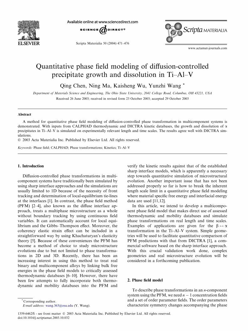
It is interesting to note that the dissolution process inthis case is not simply a reverse of growth process, and

the dissolution kinetics does not follow the parabolic

law, see Fig. 3a, which confirms Aaron and Kotler’s

analysis [30]. Due to the finite system size, soft

impingement occurs after 5 ks and gradually slows down

the dissolution process. The Al composition spikes in

the a phase region obtained from the PFM is less sharp

Fig. 3. PFM and DICTRA results for the dissolution of globular a: (a) dissolution kinetics; (b) composition profile of Al; and (c) composition profileof V.

Fig. 4. Diffusion path at 1 ks during the dissolution of globular a.

Q. Chen et al. / Scripta Materialia 50 (2004) 471–476 475

than that from DICTRA. This is understandable from

the point of view of gradient thermodynamics.

The local equilibrium at the interface is obtained

automatically in the phase field method. Again, thesystem found a different tie line from the one across the

original composition at 1223 K. Fig. 4 depicts the dif-

fusion path at 1 ks in the Ti–Al–V Gibbs triangle where

two sets of tie lines at 1173 and 1223 K are drawn. The

original compositions of a and b are located at the endsof the tie line across the overall composition (denoted by

the triangle symbol) at 1173 K, respectively. The com-

position in the b phase changes gradually by following acurved path towards the interface where the local equi-

librium prevails at a 1223 K tie line far above the one

determined by the initial composition of the a phase.The horn-shaped path forms in the a phase because thespike in the Al profile is much sharper than that for V,

which has a relatively larger mobility at 1223 K.

5. Summary

We have devised a scheme for quantitative phase field

modeling of multicomponent diffusion-controlled phase

transformations, in which both thermodynamic and ki-

netic data from existing databases can be inserted di-

rectly into the phase field model and the length and time

of the dynamic system can be readily scaled. Applica-

tions to phase transformation between a and b in Ti–Al–V in simple geometries have been proved very successful

by comparing results with that of DICTRA simulations.

The power of the phase field method relies on its cap-ability to handle arbitrarily complex geometries and this

shall be demonstrated in a forthcoming publication.

Some assumptions have been made in determining

model parameters in the method in order to have a

volume diffusion controlled process. Different assump-

tions may have to be evoked if solute drag, solute

trapping or interface-controlled process is considered.

Acknowledgements

This work is supported by AFRL under MAI grant

P035558 (QC, NM and YW) and NSF under grant

DMR 0139705 (KW) and Focused Research Group

grant DMR-0080766 (YW). We thank Wei Wang and

Sandy Ye for their valuable help with the MAI project.

References

[1] Borgenstam A, Engstr€oom A, H€ooglund L, �AAgren J. J PhaseEquilibria 2000;21:269.

[2] Wang Y, Chen LQ. Simulation of microstructural evolution using

the phase field method. In: Methods in materials research, a

current protocols. John Wiley & Sons, Inc.; 2000.

[3] Chen LQ. Ann Rev Mater Res 2002;32:113.

[4] Boettinger WJ, Warren JA, Beckermann C, Karma A. Ann Rev

Mater Res 2002;32:163.

[5] Khachaturyan AG. Theory of structural transformations in solids.

New York: John Wiley & Sons; 1983.

[6] Grafe U, Botteger B, Tiaden J, Fries SG. Scripta Mater

2000;42:1179.

[7] Cha P-R, Yeon D-H, Yoon J-K. Acta Mater 2001;49:3295.

[8] Yeon D-H, Cha P-R, Yoon J-K. Scripta Mater 2000;45:661.

[9] Zhu JZ, Liu ZK, Vaithyanathan V, Chen LQ. Scripta Mater

2002;46:401.

476 Q. Chen et al. / Scripta Materialia 50 (2004) 471–476

[10] Loginova I, Odqvist J, Amberg G, �AAgren J. Acta Mater

2003;51:1327.

[11] Shen C, Chen Q, Wang Y, Wen YH, Simmons JP. Scripta Mater,

submitted for publication.

[12] Shen C, Chen Q, Wang Y, Wen YH, Simmons JP. Scripta Mater,

submitted for publication.

[13] Wang Y, Banerjee D, Su CC, Khachaturyan AG. Acta Mater

1998;46:2983.

[14] Ansara I, Dupin N, Lukas HL, Sundman B. J Alloy Compd

1997;247:20.

[15] Toledano P, Dimitriev V. Reconstructive phase transitions: in

crystals and quasicrystals. Singapore: World Scientific; 1996.

[16] Wang S-L, Sekerka RF, Wheeler AA, Murray BT, Coriell SR,

Braun RJ, et al. Physica D 1993;69:189.

[17] Warren JA, Boettinger WJ. Acta Metall Mater 1995;43:689.

[18] Cahn JW, Hilliard JE. J Chem Phys 1958;28:258.

[19] Allen SM, Cahn JW. Acta Metall 1979;27:1085.

[20] Gunton JD, Miguel MS, Sahni PS. The dynamics of first-order

phase transitions. In: Domb C, Lebowitz JL, editors. Phase

transitions and critical phenomena, vol. 8. New York: Academic

Press; 1983.

[21] Cahn JW. Acta Metall 1961;9:795.

[22] Kirkaldy JS, Young DJ. Diffusion in the condensed state.

London: Institute of Metals; 1987.

[23] Andersson J-O, �AAgren J. J Appl Phys 1992;72:1350.

[24] Zhang F. CompuTherm, LLC, USA, 2002, private communica-

tion.

[25] Chen Q, Wang Y. in preparation (data available upon request).

[26] Mullins WW, Sekerka RF. J Appl Phys 1963;34:323.

[27] Townsend RD, Kirkaldy JS. Trans ASM 1968;61:605.

[28] Aaronson HI, Spanos G, Masamura RA, Vardiman RG, Moon

DW, Menon ESK, et al. Mater Sci Eng, B 1995;32:107.

[29] Menon ESK, Aaronson HI. Metall Trans A 1986;17A:1703.

[30] Aaron HB, Kotler GR. Metall Trans 1971;2:393.