quantitative methods and computer applications in the historical and social sciences roman studer...
Post on 18-Dec-2015
218 views
TRANSCRIPT
Quantitative Methods and Computer Applications in
the Historical and Social
SciencesRoman Studer
Nuffield [email protected]
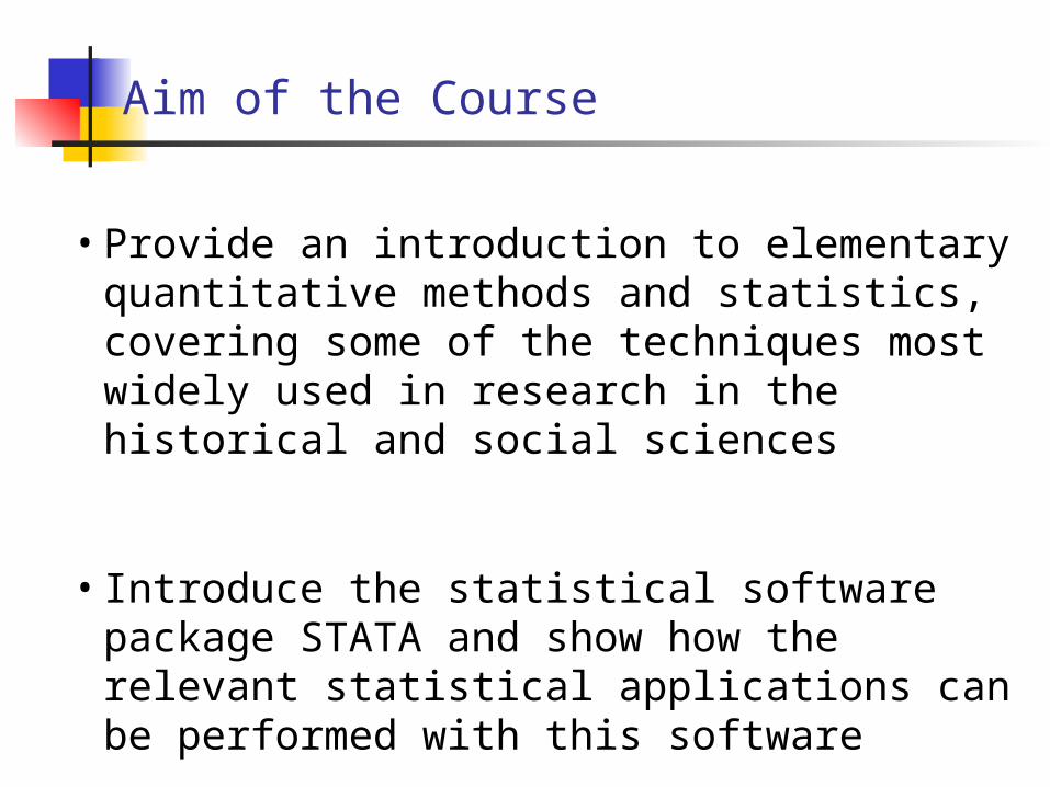
Aim of the Course
• Provide an introduction to elementary quantitative methods and statistics, covering some of the techniques most widely used in research in the historical and social sciences
• Introduce the statistical software package STATA and show how the relevant statistical applications can be performed with this software

Motivation of the Course
• Understanding quantitative research Quantitative methods are widely used both in History as well as in (other)
Social Sciences Being able to make use of quantitative research, but also being able to
assess its limits
• Using quantitative methods in your own research How representative or reliable are observed patterns? If many factors determine an outcome, the relative importance of the factors
can be determined Graphs and tables can be very persuasive tools, they can also give valuable
hints and raise new questions
• General usage We live in a “data world”, hence being able to handle data and quantitative
studies properly is a very useful qualification both in the job market as well as for everyday life
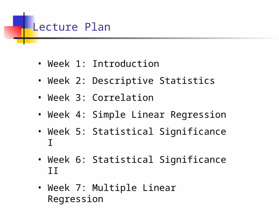
Lecture Plan
• Week 1: Introduction
• Week 2: Descriptive Statistics
• Week 3: Correlation
• Week 4: Simple Linear Regression
• Week 5: Statistical Significance I
• Week 6: Statistical Significance II
• Week 7: Multiple Linear Regression
• Week 8: Dummy Variables
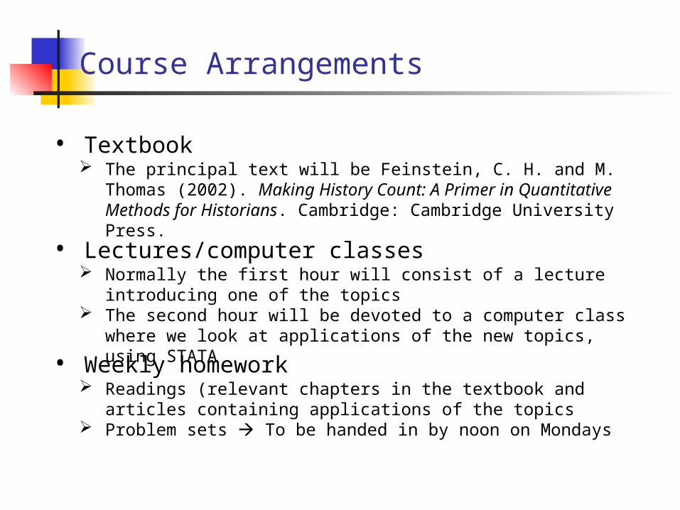
Course Arrangements
• Lectures/computer classes Normally the first hour will consist of a lecture introducing one of the topics The second hour will be devoted to a computer class where we look at
applications of the new topics, using STATA
• Textbook The principal text will be Feinstein, C. H. and M. Thomas (2002). Making
History Count: A Primer in Quantitative Methods for Historians. Cambridge: Cambridge University Press.
• Weekly homework Readings (relevant chapters in the textbook and articles containing
applications of the topics Problem sets To be handed in by noon on Mondays
Course Arrangements (II)
• All information is available on the course’s website:http://www.nuff.ox.ac.uk/users/studer/teaching.htmincluding slides, problem sets and data sets
• Mock exam At the end of the course there will be a simple take-away examination to
test your understanding of the various concepts and procedures covered during the course
Your Input
• Any questions so far?
• Any comments?
• Short introduction of participants What’s your background and how much do you know already
about statistics and quantitative methods? Why are you taking the course? Are you planning to use quantitative methods in your research? Is there anything specific you want to learn that is not on the
program?
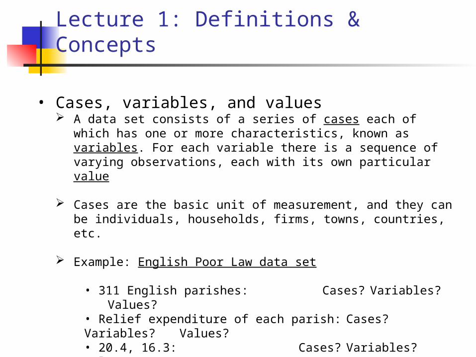
Lecture 1: Definitions & Concepts
• Cases, variables, and values A data set consists of a series of cases each of which has one or more
characteristics, known as variables. For each variable there is a sequence of varying observations, each with its own particular value
Cases are the basic unit of measurement, and they can be individuals, households, firms, towns, countries, etc.
Example: English Poor Law data set
• 311 English parishes: Cases? Variables? Values?• Relief expenditure of each parish: Cases? Variables? Values?• 20.4, 16.3: Cases? Variables? Values?
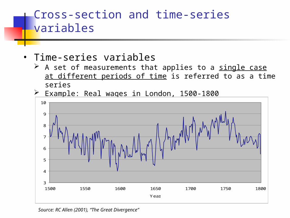
Cross-section and time-series variables
• Time-series variables A set of measurements that applies to a single case at different periods of time
is referred to as a time series Example: Real wages in London, 1500-1800
3
4
5
6
7
8
9
10
1500 1550 1600 1650 1700 1750 1800
Year
Source: RC Allen (2001), “The Great Divergence”
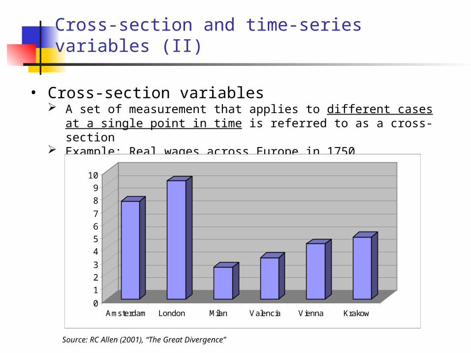
Cross-section and time-series variables (II)
• Cross-section variables A set of measurement that applies to different cases at a single point in time is
referred to as a cross-section Example: Real wages across Europe in 1750
Source: RC Allen (2001), “The Great Divergence”
0
1
2
3
4
5
6
7
8
9
10
Amsterdam London Milan Valencia Vienna Krakow
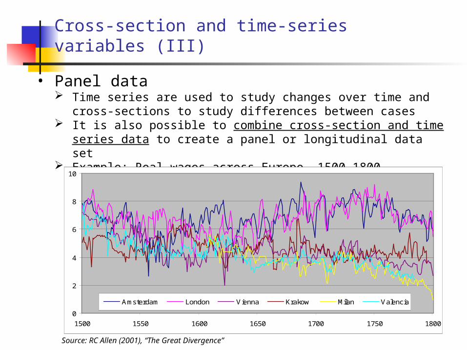
Cross-section and time-series variables (III)
• Panel data Time series are used to study changes over time and cross-sections to study
differences between cases It is also possible to combine cross-section and time series data to create a
panel or longitudinal data set Example: Real wages across Europe, 1500-1800
0
2
4
6
8
10
1500 1550 1600 1650 1700 1750 1800
Amsterdam London Vienna Krakow Milan Valencia
Source: RC Allen (2001), “The Great Divergence”
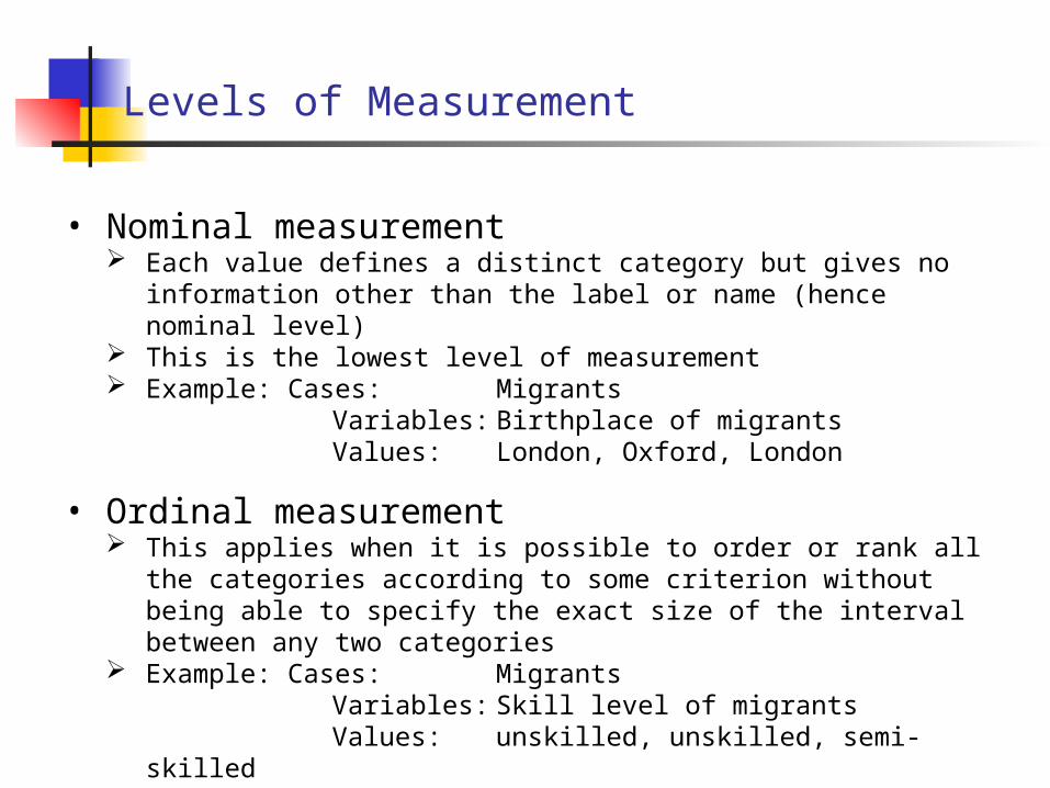
Levels of Measurement
• Nominal measurement Each value defines a distinct category but gives no information other than the
label or name (hence nominal level) This is the lowest level of measurement Example: Cases: Migrants
Variables: Birthplace of migrantsValues: London, Oxford, London
• Ordinal measurement This applies when it is possible to order or rank all the categories according to
some criterion without being able to specify the exact size of the interval between any two categories
Example: Cases: MigrantsVariables: Skill level of migrantsValues: unskilled, unskilled, semi-skilled
Levels of Measurement
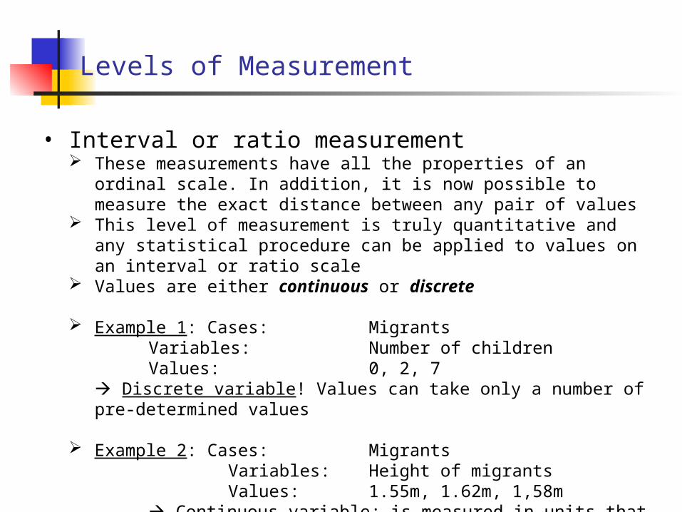
• Interval or ratio measurement These measurements have all the properties of an ordinal scale. In addition, it is
now possible to measure the exact distance between any pair of values This level of measurement is truly quantitative and any statistical procedure can
be applied to values on an interval or ratio scale Values are either continuous or discrete
Example 1: Cases: MigrantsVariables: Number of childrenValues: 0, 2, 7
Discrete variable! Values can take only a number of pre-determined values
Example 2: Cases: MigrantsVariables: Height of migrantsValues: 1.55m, 1.62m, 1,58m
Continuous variable; is measured in units that can (theoretically) be reduced in size to an infinite degree
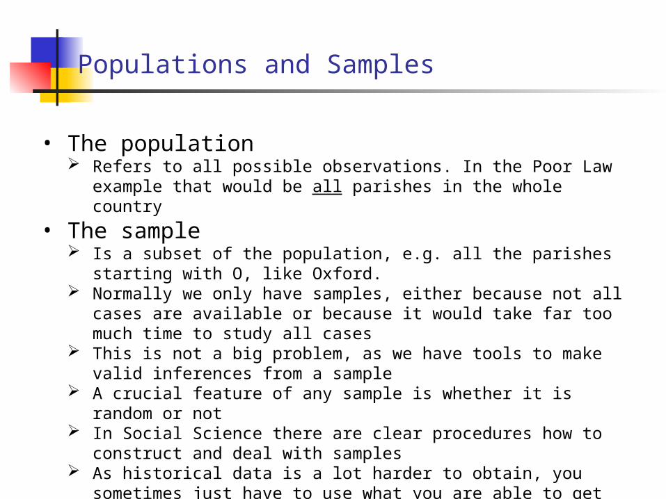
Populations and Samples
• The population Refers to all possible observations. In the Poor Law example that would be all
parishes in the whole country
• The sample Is a subset of the population, e.g. all the parishes starting with O, like Oxford. Normally we only have samples, either because not all cases are available or
because it would take far too much time to study all cases This is not a big problem, as we have tools to make valid inferences from a
sample A crucial feature of any sample is whether it is random or not In Social Science there are clear procedures how to construct and deal with
samples As historical data is a lot harder to obtain, you sometimes just have to use what
you are able to get
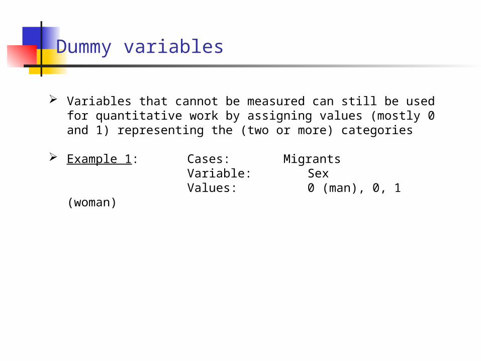
Dummy variables
Variables that cannot be measured can still be used for quantitative work by assigning values (mostly 0 and 1) representing the (two or more) categories
Example 1: Cases: MigrantsVariable: SexValues: 0 (man), 0, 1 (woman)
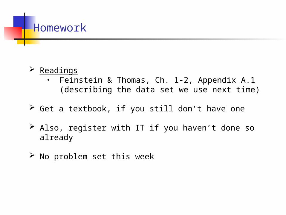
Homework
Readings• Feinstein & Thomas, Ch. 1-2, Appendix A.1 (describing the data
set we use next time)
Get a textbook, if you still don’t have one
Also, register with IT if you haven’t done so already
No problem set this week