Quantitative Easing and Financial Stability∗

Michael WoodfordColumbia University

May 13, 2016

Abstract

The massive expansion of central-bank balance sheets in response to recentcrises raises important questions about the effects of such “quantitative easing”policies, both their effects on financial conditions and on aggregate demand (theintended effects of the policies), and their possible collateral effects on financialstability. The present paper compares three alternative dimensions of central-bank policy — conventional interest-rate policy, increases in the central bank’ssupply of safe (monetary) liabilities, and macroprudential policy (possibly im-plemented through discretionary changes in reserve requirements) — showingin the context of a simple intertemporal general-equilibrium model why theyare logically independent dimensions of variation in policy, and how they jointlydetermine financial conditions, aggregate demand, and the severity of the risksassociated with a funding crisis in the banking sector. In the proposed model,each of the three dimensions of policy can be used independently to influenceaggregate demand, and in each case a more stimulative policy also increasesfinancial stability risk. However, the policies are not equivalent, and in par-ticular the relative magnitudes of the two kinds of effects are not the same.Quantitative easing policies increase financial stability risk (in the absence ofan offsetting tightening of macroprudential policy), but they actually increasesuch risk less than either of the other two policies, relative to the magnitudeof aggregate demand stimulus; and a combination of expansion of the centalbank’s balance sheet with a suitable tightening of macroprudential policy canhave a net expansionary effect on aggregate demand with no increased risk tofinancial stability. This suggests that quantitative easing policies may be usefulas an approach to aggregate demand management not only when the zero lowerbound precludes further use of conventional interest-rate policy, but also whenit is not desirable to further reduce interest rates because of financial stabilityconcerns.

∗I would like to thank Vasco Curdia, Emmanuel Farhi, Robin Greenwood, Ricardo Reis, HeleneRey, and Lars Svensson for helpful comments, Chengcheng Jia and Dmitriy Sergeyev for excellentresearch assistance, and the National Science Foundation for supporting this research.

Since the global financial crisis of 2008-09, many of the leading central banks

have dramatically increased the size of their balance sheets, and also have shifted

the composition of the assets that they hold, toward greater holdings of longer-term

securities (as well as toward assets that are riskier in other respects). While many

have hailed these policies as contributing significantly to contain the degree of damage

to both the countries’ financial systems and real economies resulting from the collapse

of confidence in certain types of risky assets, the policies have also been and remain

quite controversial. One of the concerns raised by skeptics has been the suggestion

that such “quantitative easing” by central banks may have been supporting countries’

banking systems and aggregate demand only by encouraging risk-taking by ultimate

borrowers and by financial intermediaries of a kind that increases the risk of precisely

the sort of destructive financial crisis that had led these policies to be introduced.

The most basic argument for suspecting that such policies create risks to financial

stability is simply that, according to proponents of these policies in the central banks

(e.g., Bernanke, 2012), they represent alternative means of achieving the same kind

of relaxation of financial conditions that would under more ordinary circumstances

be achieved by lowering the central bank’s operating target for short-term interest

rates — but a means that continues to be available even when short-term nominal

interest rates have already reached their effective lower bound, and so cannot be

lowered to provide further stimulus. If one believes that cuts in short-term interest

rates have as a collateral effect — or perhaps even as the main channel through which

they affect aggregate demand, as argued by Adrian and Shin (2010) — an increase

in the degree to which intermediaries take more highly leveraged positions in risky

assets, increasing the likelihood of and/or severity of a potential financial crisis, then

one might suppose that to the extent that quantitative easing policies are effective

in relaxing financial conditions in order to stimulate aggregate demand, they should

similarly increase risks to financial stability.

One might go further and argue that such policies relax financial conditions by

increasing the supply of central-bank reserves,1 and one might suppose that such

an increase in the availability of reserves matters for financial conditions precisely

because it relaxes a constraint on the extent to which private financial intermediaries

1The term “quantitative easing,” originally introduced by the Bank of Japan to describe the

policy that it adopted in 2001 in attempt to stem the deflationary slump that Japan had suffered in

the aftermath of the collapse of an asset bubble in the early 1990s, refers precisely to the intention to

increase the monetary base (and hence, it was hoped, the money supply more broadly) by increasing

the supply of reserves.

1

can issue money-like liabilities (that are subject to reserve requirements) as a way

of financing their acquisition of more risky and less liquid assets, as in the model of

Stein (2012). Under this view of the mechanism by which quantitative easing works,

one might suppose that it should be even more inevitably linked to an increase in

financial stability risk than expansionary interest-rate policy (which, after all, might

also increase aggregate demand through channels that do not rely upon increased

risk-taking by banks).

Finally, some may be particularly suspicious of quantitative easing policies on

the ground that these policies, unlike conventional interest-rate policy, relax finan-

cial conditions primarily by reducing the risk premia earned by holding longer-term

securities, rather than by lowering the expected path of the risk-free rate.2 Such a

departure from the normal historical pattern of risk premia as a result of massive

central-bank purchases may seem a cause for alarm. If one thinks that the premia

that exist when market pricing is not “distorted” by the central bank’s intervention

provide an important signal of the degree of risk that exists in the marketplace, one

might fear that central-bank actions that suppress this signal — not by actually re-

ducing the underlying risks, but only by preventing them from being reflected so fully

in market prices — run the danger of distorting perceptions of risk in a way that will

encourage excessive risk-taking.

The present paper considers the extent to which these are valid grounds for concern

about the use of this policy tool by central banks, by analyzing further the mechanisms

just sketched, in the context of an explicit model of the way in which quantitative

easing policies influence financial conditions, and the way in which monetary policies

more generally affect the incentives of financial intermediaries to engage in maturity

and liquidity transformation of a kind that increases the risk of financial crisis. It

argues, in fact, that the concerns just raised are of little merit. But it does not reach

this conclusion by challenging the view that quantitative easing policies can indeed

effectively relax financial conditions (and so achieve effects on aggregate demand that

are similar to the effects of conventional interest-rate policy); nor does it deny that

risks to financial stability are an appropriate concern of monetary policy deliberations,

or that expansionary interest-rate policy tends to increase such risks (among other

2Again see Bernanke (2012) for discussion of this view of how the policies work, though he also

discusses the possibility of effects of quantitative easing that result from central-bank actions being

taken to signal different intentions regarding future interest-rate policy.

2

effects). The model developed here is one in which risk-taking by the financial sector

can easily be excessive (in the sense that a restriction on banks’ ability to engage in

liquidity transformation to the degree that they choose to under laissez-faire would

raise welfare); in which, when that is true, a reduction in short-term interest rates

through central-bank action will worsen the problem by making it even more tempting

for banks to finance acquisitions of risky, illiquid assets by issuing short-term safe

liabilities; and in which the purchase of longer-term and/or risky assets by the central

bank, financed by creating additional reserves (or other short-term safe liabilities,

such as reverse repos or central-bank bills, that would also be useful in facilitating

transactions), will indeed loosen financial conditions, with an effect on aggregate

demand that is similar, though not identical to, the effect of a reduction in the central

bank’s operating target for its policy rate. Nonetheless, we show that quantitative

easing policies should not increase risks to financial stability, and should instead tend

to reduce them.

The reason for this different conclusion hinges on our conception of the sources

of the kind of financial fragility that allowed a crisis of the kind just experienced to

occur, and the way in which monetary policy can affect the incentives to create a more

fragile financial structure. In our view, the fragility that led to the recent crisis was

greatly enhanced by the notable increase in maturity and liquidity transformation in

the financial sector in the years immediately prior to the crisis (Brunnermeier, 2009;

Adrian and Shin, 2010) — in particular, the significant increase in funding of financial

intermediaries by issuance of collateralized short-term debt, such as repos (financing

investment banks) or asset-backed commercial paper (issued by SIVs). Such financing

is relatively inexpensive, in the sense that investors will hold such instruments even

when they promise a relatively low yield, because of the assurance they provide that

the investor can be sure of payment and can withdraw their funds at any time on short

notice if desired. But too much of it is dangerous, because it exposes the leveraged

institution to funding risk, which may require abrupt de-leveraging through a “fire

sale” of relatively illiquid assets. The sudden need to sell relatively illiquid assets

in order to cover a shortfall of funding can substantially depress the price of those

assets, requiring even more de-leveraging and leading to a “margin spiral” of the

kind described by Shleifer and Vishny (1992, 2010) and Brunnermeier and Pederson

(2009).

It is important to ask why such fragile financial structures should arise as an

3

equilibrium phenomenon, in order to understand how monetary policy may increase

or decrease the likely degree of fragility. According to the perspective that we adopt

here, investors are attracted to the short-term safe liabilities created by banks or other

financial intermediaries because assets with a value that is completely certain are

more widely accepted as a means of payment.3 If an insufficient quantity of such safe

assets are supplied by the government (through means that we discuss further below),

investors will pay a “money premium” for privately-issued short-term safe instruments

with this feature, as documented by Greenwood et al. (2010), Krishnamurthy and

Vissing-Jorgensen (2012), and Carlson et al. (2014). This provides banks with an

incentive to obtain a larger fraction of their financing in this way. Moreover, they may

choose an excessive amount of this kind of financing, despite the funding risk to which

it exposes them, because each individual bank fails to internalize the effects of their

collective financing decisions on the degree to which asset prices will be depressed in

the event of a “fire sale.” This gives rise to a pecuniary externality, as a result of

which excessive risk is taken in equilibrium (Lorenzoni, 2008; Jeanne and Korinek,

2010; Stein, 2012).

Conventional monetary policy, which cuts short-term nominal interest rates in

response to an aggregate demand shortfall, can arguably exacerbate this problem, as

low market yields on short-term safe instruments will further increase the incentive

for private issuance of liabilities of this kind (Adrian and Shin, 2010; Giavazzi and

Giovannini, 2012). The question of primary concern in this paper is, do quantitative

easing policies, pursued as a means of providing economic stimulus when conventional

monetary policy is constrained by the lower bound on short-term nominal interest

rates, increase financial stability risks for a similar reason?

In the model proposed here, quantitative easing policies lower the equilibrium real

yield on longer-term and risky government liabilities, just as a cut in the central bank’s

target for the short-term riskless rate will, and this relaxation of financial conditions

has a similar expansionary effect on aggregate demand in both cases. Nonetheless,

the consequences for financial stability are not the same. In the case of conventional

monetary policy, a reduction in the riskless rate lowers the equilibrium yield on risky

assets as well because, if it did not, the increased spread between the two yields

3The role of non-state-contingent payoffs in allowing an asset to be widely acceptable as a means

of payment is stressed in particular by Gorton and Pennacchi (2010), and in recent discussions such

as Gorton (2010) and Gorton, Lewellen and Metrick (2012).

4

would provide an increased incentive for maturity and liquidity transformation on

the part of banks, which they pursue until a point at which the spread has decreased

(because of diminishing returns to further investment in risky assets) to where it

is again balanced by the risks associated with overly leveraged investment. (This

occurs, in equilibrium, partly through a reduction in the degree to which the spread

increases — which means that the expected return on risky assets is reduced — and

partly through an increase in the risk of a costly “fire sale” liquidation of assets.)

In the case of quantitative easing, instead, the equilibrium return on risky assets is

reduced, but in this case through a reduction, rather than an increase in the spread

between the two yields. The “money premium,” which results from a scarcity of safe

assets, should be reduced if the central-bank asset purchases increase the supply of

safe assets to the public, as argued by Caballero and Farhi (2013) and Carlson et al.

(2014). Hence the incentives for creation of a more fragile financial structure are not

increased as much by expansionary monetary policy of this kind.

The idea that quantitative easing policies, when pursued as an additional means

of stimulus when the risk-free rate is at the zero lower bound, should increase risks to

financial stability because they are analogous to an expansionary policy that relaxes

reserve requirements on private issuers of money-like liabilities is also based on a

flawed analogy. It is true, in the model of endogenous financial stability risk presented

here, that a relaxation of a reserve requirement proportional to banks’ issuance of

short-term safe liabilities will (in the case that the constraint binds) increase the

degree to which excessive liquidity transformation occurs. And it is also true that in

a conventional textbook account of the way in which monetary policy affects financial

conditions, an increase in the supply of reserves by the central bank relaxes the

constraint on banks’ issuance of additional money-like liabilities (“inside money”)

implied by the reserve requirement, so that the means through which the central

bank implements a reduction in the riskless short-term interest rate is essentially

equivalent to a reduction in the reduction in the reserve requirement. However, this

is not a channel through which quantitative easing policies can be effective, when the

risk-free rate has already fallen to zero (or more generally, to the level of interest paid

on reserves). For in such a case, reserves are necessarily already in sufficiently great

supply for banks to be satiated in reserves, so that the opportunity cost of holding

them must fall to zero in order for the existing supply to be voluntarily held. Under

such circumstances (which is to say, those existing in countries like the US since

5

the end of 2008), banks’ reserve requirements have already ceased to constrain their

behavior. Hence, to the extent that quantitative easing policies are of any use at the

zero lower bound on short-term interest rates, their effects cannot occur through this

traditional channel.

In the model presented here, quantitative easing is effective at the zero lower

bound (or more generally, even in the absence of reserve requirements, or under cir-

cumstances where there is already satiation in reserves); this is because an increase

in the supply of safe assets (through issuance of additional short-term safe liabili-

ties by the central bank, used to purchase assets that are not equally money-like)

reduces the equilibrium “money premium.” But whereas a relaxation of a binding

reserve requirement would increase banks’ issuance of short-term safe liabilities (and

hence financial stability risk), a reduction in the “money premium” should reduce

their issuance of such liabilities, so that financial stability risk should if anything be

reduced.

The idea that a reduction in risk premia as a result of central-bank balance-sheet

policy should imply a greater danger of excessive risk-taking is similarly mistaken.

In the model presented here, quantitative easing achieves its effects (both on the

equilibrium required return on risky assets and on aggregate demand) by lowering

the equilibrium risk premium — that is, the spread between the required return on

risky assets and the riskless rate. But this does not imply the creation of conditions

under which it should be more tempting for banks to take on greater risk. To the

contrary, the existence of a smaller spread between the expected return on risky assets

and the risk-free rate makes it less tempting to finance purchases of risky assets by

issuing safe, highly liquid short-term liabilities that need pay only the riskless rate.

Hence again a correct analysis implies that quantitative easing policies should increase

financial stability, rather than threatening it.

The remainder of the paper develops these points in the context of an explicit

intertemporal monetary equilibrium model, in which it is possible to clearly trace the

general-equilibrium determinants of risk premia, the way in which they are affected by

both interest-rate policy and the central bank’s balance sheet, and the consequences

for the endogenous capital structure decisions of banks. Section 1 presents the struc-

ture of the model, and section 2 then derives the conditions that must link the various

endogenous prices and quantities in an intertemporal equilibrium. Section 3 considers

the effects of alternative balance-sheet policies on equilibrium variables, focusing on

6

the case of a stationary long-run equilibrium with flexible prices. Section 4 compares

the ways in which quantitative easing and adjustments of reserve requirements af-

fect banks’ financing decisions. Finally, section 5 compares (somewhat more briefly)

the short-run effects of both conventional monetary policy, quantitative easing, and

macroprudential policy in the presence of nominal rigidities that allow conventional

monetary policy to affect the degree of real economic activity. Section 6 concludes.

1 A Monetary Equilibrium Model with Fire Sales

This section develops a simple model of monetary equilibrium, in which it is possible

simultaneously to consider the effects of the central bank’s balance sheet on financial

conditions (most notably, the equilibrium spread between the expected rate of return

on risky assets and the risk-free rate of interest) and the way in which private banks’

financing decisions can increase risks to financial stability. An important goal of the

analysis is to present a sufficiently explicit model of the objectives and constraints

of individual actors to allow welfare analysis of the equilibria associated with alter-

native policies that is based on the degree of satisfaction of the individual objectives

underlying the behavior assumed in the model, as in the modern theory of public

finance, rather than judging alternative equilibria on the basis of some more ad hoc

criterion.4

Risks to financial stability are modeled using a slightly adapted version of the

model proposed by Stein (2012). The Stein model is a three-period model in which

banks finance their investments in risky assets in the first period; a crisis may occur in

the second period, in which banks are unable to roll over their short-term financing

and as a result may have to sell illiquid risky assets in a “fire sale”; and in the

third period, the ultimate value of the risky assets is determined. The present model

incorporates this model of financial contracting and occasional fire sales of assets into

a fairly standard intertemporal general-equilibrium model of the demand for money-

like assets, the “cash-in-advance” model of Lucas and Stokey (1987). In this way,

the premium earned by money-like assets, that is treated as an exogenous parameter

in Stein (2012), can be endogenized, and the effects of central-bank policy on this

4The proposed framework is further developed in Sergeyev (2016), which considers the interaction

between conventional monetary policy and country-specific macroprudential policies in a currency

union.

7

variable can be analyzed, and through this the consequences for financial stability.

1.1 Elements of the Model

Like most general-equilibrium models of monetary exchange, the Lucas and Stokey

(1987) model is an infinite-horizon model, in which the willingness of sellers to accept

central-bank liabilities as payment for real goods and services in any period depends

on the expectation of being able to use those instruments as a means of payment in

further transactions in future periods. The state space of the model is kept small

(allowing a straightforward characterization of equilibrium, despite random distur-

bances each period) by assuming a representative household structure; the two sides

of each transaction involving payment using cash are assumed to be two members of

a household unit with a common objective, that can be thought of as a “worker” and

a “shopper.” During each period, the worker and shopper from a given household

have separate budget constraints (so that cash received by the worker as payment for

the sale of produced goods cannot be immediately used by the shopper to purchase

goods, in the same market), as is necessary for the “cash-in-advance” constraint to

matter; but at the end of the period, their funds are again pooled in a single house-

hold budget constraint (so that only the asset positions of households, that are all

identical, matter at this point).

We shall employ a similar device, but further increasing the number of distinct

roles for different members of the household, in order to introduce additional kinds

of financial constraints into the model, while retaining the convenience of a repre-

sentative household. We suppose that each infinite-lived household is made of four

members with different roles during the period: a “worker” who supplies the inputs

used to produce all final goods, and receives the income from the sale of these goods;

a “shopper” who purchases “regular goods” for consumption by the household, and

who holds the household’s cash balance, for use in such transactions; a “banker” who

buys risky durable goods, and issues short-term safe liabilities in order to finance

some of these purchases; and an “investor” who purchases “special” final goods, and

can also bid for the risky durables sold by bankers in the event of a fire sale.5 As

5The distinction between bankers, investors, and worker/shopper pairs corresponds to the dis-

tinction in the roles of “bankers,” “patient investors,” and “households” in the model of Stein (2012).

In the Stein model, these three types of agents are distinct individuals with no sharing of resources

among them, rather than members of a single (larger) household; the device of having them pool

8

in the Lucas-Stokey model, the different household members have separate budget

constraints during the period (which is the significance of referring to them as differ-

ent people), but pool their budgets at the end of each period in a single household

budget constraint.

Four types of final goods are produced each period: durable goods and three types

of non-durable goods, called “cash goods,” “credit goods,” and “special goods.” In

addition, we suppose that workers also produce intermediate “investment goods”

that are used as an input in the production of durable goods. Both “cash” and

“credit” goods are purchased by shoppers; the distinction between the two types of

goods is taken from Lucas and Stokey (1987), where the possibility of substitution

by consumers between the two types of goods (one subject to the cash-in-advance

constraint, the other not) allows the demand for real cash balances to vary with the

size of the liquidity premium (opportunity cost of holding cash), for a given level of

planned real expenditure. This margin of substitution also results in a distortion in

the allocation of resources that depends on the size of the liquidity premium, and

we wish to take this distortion into account when considering the welfare effects of

changing the size of the central bank’s balance sheet.

The introduction of “special goods” purchased only by the investor provides an

alternative use for the funds available to the investor, so that the amount that in-

vestors will spend on risky durables in a fire sale depends on how low the price of

the durables falls.6 The produced “durable goods” in our model play the role of the

risky investment projects in the model of Stein (2012): they require an initial outlay

of resources, financed by bankers, in order to allow the production of something that

may or may not yield a return later. The device of referring separately to investment

goods and to the durable goods produced from them allows us to treat investment

goods as perfect substitutes for cash or credit goods on the production side, allowing

a simple specification of workers’ disutility of supplying more output, without having

also to treat durable goods as perfect substitutes for those goods, which would not

allow the relative price of durables to rise in a credit boom.

assets at the end of each “period” is not needed to simplify the model dynamics, because the model

simply ends when the end of the first and only “period” is reached (in the sense in which the term

“period” is used in this model). Note that in the present model, the representative household device

also allows more unambiguous welfare comparisons among equilibria.6The opportunity of spending on purchases of special goods plays the same role in our model as

the possibility of investment in “late-arriving projects” in the model of Stein (2012).

9

All of the members of a given household are assumed to act so as to maximize a

common household objective. Looking forward from the beginning of any period t,

the household objective is to maximize

Et

∞∑τ=t

βτ−t [u(c1τ , c2τ ) + u(c3τ ) + γsτ − v(Yτ ) − w(xτ )]. (1.1)

Here c1t, c2t, c3t denote the household’s consumption of cash goods, credit goods, and

special goods respectively in period t; st denotes the quantity of durables held by the

household at the end of period t that have not proven to be worthless, and hence

the flow of services in period t from such intact durables; Yt denotes the household’s

supply of “normal goods” (a term used collectively for cash goods, credit goods, and

investment goods, that are all perfect substitutes from the standpoint of a producer)

in period t; and xt denotes the household’s supply of special goods in period t.

The functions u(·, ·), u(·), v(·), and w(·) are all increasing functions of each of their

arguments; the functions u(·, ·) and u(·) are strictly concave; and the functions v(·)and w(·) are at least weakly convex. We also assume that the function u(·, ·) implies

that both cash and credit goods are normal goods, in the sense that it will be optimal

to increase purchases of both types of goods if a household increases its expenditure

on these types of goods in aggregate, while the (effective) relative price of the two

types of goods remains the same.7 In addition, the discount factor satisfies 0 < β < 1,

and γ > 0. The operator Et[·] indicates the expectation conditional on information

at the beginning of period t.

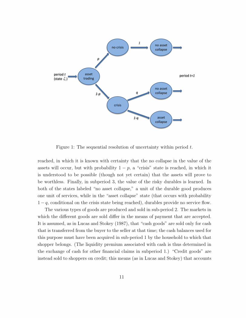
Each of the infinite sequence of periods t = 0, 1, 2, . . . is subdivided into three

subperiods, corresponding to the three periods in the model of Stein (2012). The

sequence of events, and the set of alternative states that may be reached, within

each period is indicated in Figure 1. In subperiod 1, a financial market is open

in which bankers issue short-term safe liabilities and acquire risky durables, and

households decide on the cash balances to hold for use by the shopper.8 In subperiod

2, information is revealed about the possibility that the durable goods purchased

by the banks will prove to be valueless. With probability p, the “no crisis” state is

7By the effective relative price we mean the relative price taking into account the cost to the

household of having to hold cash in order to purchase cash goods, as discussed further below.8This sub-period corresponds both to the first period of the Stein (2012) model, in which risky

projects are financed, and to the securities-trading subperiod of the model in section 5 of Lucas and

Stokey (1987), in which bonds are priced and hence the liquidity premium on cash is determined.

10

assettrading

no crisisno assetcollapse

crisis

no assetcollapse

assetcollapse

period t(state )tξ

period t+1

1

q

1-q

p

1-p

Figure 1: The sequential resolution of uncertainty within period t.

reached, in which it is known with certainty that the no collapse in the value of the

assets will occur, but with probability 1 − p, a “crisis” state is reached, in which it

is understood to be possible (though not yet certain) that the assets will prove to

be worthless. Finally, in subperiod 3, the value of the risky durables is learned. In

both of the states labeled “no asset collapse,” a unit of the durable good produces

one unit of services, while in the “asset collapse” state (that occurs with probability

1− q, conditional on the crisis state being reached), durables provide no service flow.

The various types of goods are produced and sold in sub-period 2. The markets in

which the different goods are sold differ in the means of payment that are accepted.

It is assumed, as in Lucas and Stokey (1987), that “cash goods” are sold only for cash

that is transferred from the buyer to the seller at that time; the cash balances used for

this purpose must have been acquired in sub-period 1 by the household to which that

shopper belongs. (The liquidity premium associated with cash is thus determined in

the exchange of cash for other financial claims in subperiod 1.) “Credit goods” are

instead sold to shoppers on credit; this means (as in Lucas and Stokey) that accounts

11

are settled between buyers and sellers only at the end of the period, at which point

the various household members have again pooled their resources, so that charges by

shoppers during the period can be paid out of the income received by workers for

goods sold during that same period. The only constraint on the amount of credit of

this kind that a household can draw upon is assumed to be determined by a no-Ponzi

condition (that is, the requirement that a household’s debts be able to be paid off

eventually out of future income, rather than rolled over indefinitely). “Investment

goods” are sold on credit in the same way. “Special goods” are also assumed to be

sold on credit, but in this case, the amount of credit that investors can draw upon is

limited by the size of the line of credit arranged for them in subperiod 1. In particular,

it is assumed that a given credit limit must be negotiated by the household before

it is learned whether a crisis will occur in subperiod 2, and thus whether investors

will have an opportunity to bid on “fire sale” assets. The existence of the non-state-

contingent credit limit for purchases by investors (both their purchases of special

goods and their purchases of risky durables liquidated by the bankers in a fire sale)

is important in order to capture the idea that only a limited quantity of funds can

be mobilized (by potential buyers with the expertise required to evaluate the assets)

to bid on the assets sold in a fire sale.9

The nature of the “cash” that can be used to purchase cash goods requires further

comment. Unlike Lucas and Stokey, we do not assume that only monetary liabilities

of the government constitute “cash” that is acceptable as a means of payment in this

market. We instead identify “cash” with the class of short-term safe instruments

(STSIs) discussed by Carlson et al. (2014) in the case of the U.S., which includes

U.S. Treasury bills (and not simply monetary liabilities of the Federal Reserve), and

certain types of collateralized short-term debt of private financial institutions. The

assumption that only these assets can be used to purchase cash goods is intended to

stand in for the convenience provided by these special instruments, that accounts for

their lower equilibrium yields relative to the short-period holding returns on other

assets.10 The fact that all assets of this type, whether issued by the government (or

9In the model of Stein (2012), this limit is ensured by assuming that the “patient investors” have

a budget that is fixed as a parameter of the model. Here we endogenize this budget, by allowing

it to be chosen optimally by the household in subperiod 1; but it is important that we still assume

that it cannot be changed in subperiod 2.10One interpretation of the “cash-in-advance” constraint is that it actually represents a constraint

on the type of assets that can be held by money-market mutual funds (MMMFs). But such a

12

central bank) or by bankers, are assumed equally to satisfy the constraint is intended

to capture the way in which the demand for privately-issued STSIs is observed to

vary with the supply of publicly-issued STSIs, as shown by Carlson et al. (2014).

We do not, of course, deny that there are also special uses for base money (currency

and reserve balances held at the Fed) as a means of payment, of the kind that Lucas

and Stokey sought to model. In particular, when the supply of reserves by the Fed

is sufficiently restricted, as was chronically the case prior to the financial crisis of

2008, the special convenience of reserve balances in facilitating payments between

financial intermediaries results in a spread between the yield on reserves and that on

STSIs such as Treasury bills; and the control of this spread by varying the supply of

reserves was the focus of monetary policy prior to the crisis. Nonetheless, the spread

between the yield on reserves and the T-bill rate (or federal funds rate) is not the one

of interest to us here. Under the circumstances in which the Fed has conducted its

experiments with “quantitative easing,” the supply of reserves has been consistently

well beyond the level needed to drive the T-bill yield down to (or even below) the

yield on reserves. Hence while certain kinds of payments by banks are constrained by

their reserve balances, we may assume that this has not been a binding constraint in

the period in which we wish to consider the effects of further changes in the central-

bank balance sheet. And granting that reserves have special uses that can result

in a liquidity premium specific to them (under circumstances no longer relevant at

present) does not in any way imply that STSIs cannot also have special uses for which

other assets will not serve, giving rise to another sort of money premium — one that

need not be zero simply because the premium associated with reserve balances has

been eliminated.

The acceptability of a financial claim as “cash” that can be used to purchase cash

goods is assumed to depend on its having a value at maturity that is completely

certain, rather than being state-contingent. This requires not only that it be a claim

to a fixed nominal quantity at a future date, but that it be viewed as completely

safe, for one of two possible reasons: either it is a liability of the government (or

constraint gives rise to a “money premium” only to the extent that there are special advantages

to investors of holding wealth in MMMFs; the ability to move funds quickly from them to make

purchases is one such advantage. Rather than explicitly introducing a demand for cash on the

part of MMMFs and assuming that households use their MMMF balances to make certain types

of purchases, we obtain the same equilibrium money premium more simply by supposing that the

STSIs can directly be used as a means of payment in certain transactions.

13

central bank),11 or it is collateralized in a way that allows a holder of the claim to

be certain of realizing a definite nominal value from it. We suppose that bankers can

issue liabilities that will be accepted as cash, but that these liabilities will have to be

backed by specific risky durables as collateral, and that the holder of the debt has the

right to demand payment of the debt at any time, if they cease to remain confident

that the collateral will continue to guarantee the fixed value for it.

When bankers purchase risky durables in the first subperiod, they can finance

some portion of the purchase price by issuing safe debt (that can be used by the

holder during the second sub-period to purchase cash goods), collateralized by the

durables that are acquired. If in the second subperiod, the “no-crisis” state is reached,

the durables can continue to serve as collateral for safe debt, as the value of the

asset in the third subperiod can in this case be anticipated with certainty. In this

case, bankers are able to roll over their short-term collateralized debt, and continue

to hold the durables. If instead the “crisis” state is reached, the durables can no

longer collateralize safe debt, as there is now a positive probability that in the third

subperiod the durables will be worthless. In this case, holders of the safe debt demand

repayment in the second sub-period, and the bankers must sell durables in a fire sale,

in the amount required to pay off the short-term debt. It is the right to force this

liquidation that makes the debt issued by bankers in the first sub-period safe.

To be more specific, we suppose that the sale of goods (and in particular, cash

goods) occurs at the beginning of the second subperiod: after it has been revealed

whether the crisis state will occur, but before the decision whether to demand imme-

diate repayment of the short-term debt is made. Thus at the time that shoppers seek

to purchase cash goods, they may hold liabilities issued by bankers that grant the

holder the right to demand repayment at any time; it is the fact that the short-term

debt has this feature that allows it to be accepted as cash in the market for cash

goods. After the market for cash goods has taken place, the holders of the bankers’

short-term debt (who may now include the sellers of cash goods) decide whether to

demand immediate repayment of the debt. At this point, these holders (whether

shoppers or workers) only care about the contribution that the asset will make to

11Of course, a claim on a government need not be completely safe. If, however, a government

borrows in its own fiat currency, and if it is committed to ensure that its nominal liabilities are

paid with certainty (by monetizing them if necessary), then it is possible for it to issue debt that is

correctly viewed as completely safe (in nominal terms).

14

the household’s pooled end-of-period budget. In the crisis state, they will choose

to demand repayment, since this ensures them the face value of the debt, whereas

if they do not demand repayment, they will receive the face value of the debt with

probability q < 1, but will receive nothing if the “asset collapse” state occurs. If they

demand repayment, they receive a claim on the investors who purchase the collateral

in the fire sale; such a claim is assumed to guarantee payment in the end-of-period

settlement, if within the bound of the line of credit arranged for the investor in the

first subperiod.

The other source of assets that count as cash is the government. Some very

short-term government liabilities (Treasury bills) count as cash. In addition, we shall

suppose that the central bank can issue liabilities that also count as cash. If the central

bank increases its supply of SFSIs by purchasing Treasury bills (that are themselves

SFSIs), the overall supply of cash will be unchanged. (This is again a demonstration

that our concept of “cash” differs importantly from that of Lucas and Stokey.) But if

the central bank purchases non-cash assets (either longer-term Treasury bonds, that

are less able to facilitate transactions than are shorter-term bills, or assets subject

to other kinds of risk) and finances these purchases by creating new short-term safe

liabilities, it can increase the net supply of SFSIs. We are interested in the effects of

this latter kind of policy.

1.2 Budget Constraints and Definition of Equilibrium

Each household begins period t with It−1 units of the investment good (purchased

in the previous period) and financial wealth At, which may represent either claims

on the government or on other households, and is measured in terms of the quantity

of cash that would have the same market value in subperiod 1 trading (even though

the assets aggregated in At need not all count as cash). In the first subperiod, the

investment good is used to produce F (It−1) units of the durable good, which can

sold on a competitive market at price Qt per unit.12 The banker in each household

purchases a quantity st of these durables, financed partly from funds provided by the

household for this purpose, and partly by issuing short-term collateralized debt in

12We may alternatively suppose that the investment goods are purchased by construction firms

that produce the durables and sell them to bankers, and that households simply begin the period

owning shares in these construction firms. The explicit introduction of such firms would not change

the equilibrium conditions presented below.

15

quantity Dt. Here Dt is the face value of the debt, the nominal quantity to which the

holder is entitled (with certainty) in the settlement of accounts at the end of period t.

The price Qt of the risky asset is quoted in the same (nominal, end-of-period) units;

thus the quantity of funds that the household must provide to the banker is equal to

Qtst −Dt in those units.

The household’s other uses of its beginning-of-period financial wealth are to ac-

quire cash, in quantity Mt, for use by the shopper, or to acquire (longer-term) bonds

Bt, which are government liabilities that do not count as cash. The quantity Mt rep-

resents the end-of-period nominal value of these safe assets; thus if interest is earned

on cash (as we allow), Mt represents the value of the household’s cash balances inclu-

sive of the interest earned on them, rather than the nominal value at the time that

they are acquired.13 The quantity of bonds Bt is measured in terms of the number

of units of cash that have the same market value in subperiod 1 trading (as with the

measurement of At). Hence the household’s choices of st, Dt, Mt and Bt in the first

subperiod are subject to an interim budget constraint

(Qtst − Dt) + Mt + Bt ≤ At + QtF (It−1). (1.2)

The financing decisions of bankers are also subject to a constraint that safe debt

Dt cannot be issued in a quantity beyond that for which they can provide sufficient

collateral, given their holdings of the durable st.14 This requires that

Dt ≤ Γt st, (1.3)

where Γt is the market price of the durable good in the fire sale, should one occur in

period t. (Here Γt is quoted in terms of the units of nominal value to be delivered by

13If we think of cash as Treasury bills, Mt represents their face value at maturity, rather than the

discounted value at which they are purchased.14We might suppose that bankers can also issue debt that is not collateralized, or not collateralized

to this extent. But such liabilities would not be treated as cash by the households that acquire them,

so that allowing such debt to be issued by a banker would have no consequences any different from

allowing the household itself to issue such debt in the first subperiod, in order to finance a larger

equity contribution to its banker. And allowing households to trade additional kinds of non-cash

financial liabilities would make no difference for the equilibrium conditions derived here; it would

simply allow us to price the additional types of financial claims. The ability of bankers to issue

collateralized short-term debt that counts as cash instead matters; this is not a type of claim that

a household can issue other than by having its banker issue it (because it must be collateralized by

risky durable goods), and issuing such claims has special value because they can relax the cash-in-

advance constraint.

16

investors in the end-of-period settlement of accounts. Note that while it is not yet

known in subperiod 1 whether a crisis will occur, the price Γt that will be realized

in the fire sale if one occurs is perfectly forecastable.) Constraint (1.3) indicates the

amount of collateral required to ensure that whichever state is reached in subperiod

2, the value of the collateralized debt will equal Dt, since sale of the collateral in a

fire sale will yield at least that amount.

Regardless of the state reached in subperiod 2, cash goods purchases of the shopper

must satisfy the cash-in-advance constraint

Pt c1t ≤ Mt, (1.4)

where Pt is the price of “normal goods” in period t (that may depend on the state

reached in subperiod 2), quoted in units of the nominal value to be delivered in the

end-of-period settlement. It is this constraint that provides a reason for the household

to choose to hold cash balances Mt. The common price for all normal goods follows

from the fact that these goods are perfect substitutes from the point of view of their

producers (workers), and that all payments that guarantee the same nominal value

in the end-of-period settlement are of equal value to the sellers, once the problem of

verifying the soundness of payments made in the cash goods market has been solved.15

There is no similar constraint on credit goods or investment goods purchases by

the shopper, as these are sold on credit. The investor’s purchases c3t of special goods,

and purchases s∗dt of durables in the fire sale16 must however satisfy a state-contingent

budget constraint

Pt c3t + ηt Γt s∗dt ≤ Ft, (1.5)

where Pt is the price of special goods (in the same units as Pt, and that similarly

may depend on the state reached in subperiod 2); ηt is an indicator variable for the

occurrence of a crisis in period t;17 and Ft is the line of credit arranged for the investor

in subperiod 1, quoted in units of the nominal quantity that the investor can promise

15Cash goods and credit goods sell for the same price in any given period for the same reason in

the model of Lucas and Stokey (1987).16We use the notation s∗t for the quantity of durables liquidated in the fire sale, if one occurs

in period t. An additional superscript d is used for the quantity demanded on this market, and a

superscript s for the quantity supplied. Note that s∗dt and s∗st are two independent choice variables

for an individual household, and need not be chosen to be equal, even though in equilibrium they

must be equal (given common choices by all households) in order for the market to clear.17That is, ηt = 1 if a crisis occurs, while ηt = 0 if the no-crisis state is reached.

17

to deliver in the end-of-period settlement, and with a value that must be independent

of the state that is realized in subperiod 2. (Note that (1.5), like (1.4), is actually

two constraints, one for each possible state that may be reached in subperiod 2.)

If the crisis state is reached in subperiod 2, the banker offers s∗st units of the

durable for sale in the fire sale, which quantity must satisfy the bounds

Dt ≤ Γt s∗st ≤ Γt st. (1.6)

The first inequality indicates that the banker must liquidate assets sufficient to allow

repayment of the short-term debt (given that in this state, the holders will necessarily

demand immediate repayment); the second inequality follows from the fact that the

banker cannot offer to sell more shares of the durable than she owns. (The range

of possible quantity offers defined in (1.6) is non-empty only because (1.3) has been

satisfied; thus a plan that satisfies (1.6) necessarily satisfies (1.3), making the earlier

constraint technically redundant.)

Given these decisions, the durables owned by the household in subperiod 3 will

equal

st = st + ηt [s∗dt − s∗st ] (1.7)

if the durables prove to be valuable, while st = 0 regardless of the household decisions

in the “asset collapse” state. The household’s pooled financial wealth at the end of

the period (in nominal units) will be given by

Wt = Mt + (Rbt/R

mt )Bt + PtYt − Pt[c1t+ c2t+It] + Ptxt + ηtΓts

∗st − Dt − Ft + Tt.

(1.8)

This consists of the household’s cash balances at the end of subperiod 1, plus the end-

of-period value of the bonds that it holds at the end of subperiod 1, plus additional

funds obtained from the sale of both normal goods and special goods in subperiod 2,

plus funds raised in the fire sale of assets in the event of a crisis, minus the household’s

expenditure on normal goods of the various types in subperiod 2, and the amounts

that it must repay at the end of the period (if not sooner) to pay off the collateralized

debt issued by the banker, and to pay for the line of credit arranged for the investor,

plus the nominal value Tt of net transfers from the government. We assume that the

household must pay Ft regardless of the extent to which the line of credit is used; we

then do not need to subtract expenditure by the investor, as this has already been

18

paid for when Ft is paid.18 Note also that bonds that cost the same amount as one

unit of cash in subperiod 1 are worth as much as Rbt/R

mt units of cash at the end of

the period, where Rmt is the gross nominal yield on cash (assumed to be known when

the cash is acquired in subperiod 1, since these assets are riskless in nominal terms)

and Rbt is the gross nominal holding return on bonds (which may depend on the state

reached by the end of the period).

We assume that each household is subject to a borrowing limit

Wt ≥ Wt, (1.9)

expressed as a lower bound on its net worth after the end-of-period settlement of

accounts. (We do not further specify the precise value of the borrowing limit, but note

that it can be set tight enough to ensure that any end-of-period net indebtedness can

eventually be repaid while at the same time being loose enough so that the constraint

(1.9) never binds in any period.) Finally, the household carries into period t+ 1 the

investment goods It purchased in subperiod 2 of period t, and financial wealth in the

amount

At+1 = Rmt+1Wt, (1.10)

where the multiplicative factor Rmt+1 converts the value of the household’s financial

wealth at the beginning of period t+ 1 into an equivalent quantity of cash (measured

in terms of the face value of the STSIs rather than their cost in subperiod 1 trading).

A feasible plan for a household is then a specification of the quantitiesMt, Bt, st, Dt,

Ft, s∗st , s

∗dt for each period t, as a function of the history ξt of shocks up until then,

and a specification of the quantities c1t, c2t, c3t, It, Yt, xt for each period t, as a func-

tion of both ξt and ηt (that is, whether a crisis occurs in period t), that satisfies the

constraints (1.2)–(1.3) for each possible history ξt and the constraints (1.4)–(1.10) for

18The assumption that Ft must be paid whether or not the full line of credit is used is important

because it prevents the household from simply asking for a large line of credit, as much as would be

desired in the crisis state, and then not using all of it in the non-crisis state. If that were possible

at no cost, the non-state-contingency of the credit available to the investor would have no bite.

The assumption that the line of credit must be paid for whether used or not makes this costly, and

results in the household’s wishing ex post in the crisis state that it had provided more funds to the

investor — though it also wishes ex post in the non-crisis state that it had provided less credit to

the investor. This device implies that the credit available to the investor will be optimal on average,

though not optimal in each state because it cannot be state-contingent.

19

each possible history (ξt, ηt), given initial financial wealth A0 and pre-existing invest-

ment goods I−1, and given the state-contingent evolution of the prices, net transfers

from the government to households, and the borrowing limit. An optimal plan is a

feasible plan that maximizes (1.1).

Equilibrium requires that all markets for goods and assets clear. Thus it requires

that in the first subperiod of period t,

Mt = Mt + Dt, (1.11)

Bt = Bst , (1.12)

st = F (It−1), (1.13)

where Mt is the public supply of cash (short-term safe liabilities of the government

or of the central bank) and Bst is the supply of longer-term government bonds (not

held by the central bank). Note that we assume for simplicity that durables fully

depreciate after supplying a service flow (in the event that there is no asset collapse)

in the period in which they are produced and acquired by bankers; thus the supply of

durables to be acquired by bankers in period t is given simply by the new production

F (It−1), and is independent of the quantity st−1 of valuable durables in the previous

period.

Equilibrium also requires that in the second subperiod, if a crisis occurs,

s∗dt = s∗st , (1.14)

and that in either the crisis or in the non-crisis state,

c1t + c2t + It = Yt, (1.15)

and

c3t = xt. (1.16)

We can then define a (flexible-price) equilibrium as a specification of prices Qt,Γt

and yield Rmt on cash for each history ξt, and prices Pt, Pt and bond yields Rb

t for

each history (ξt, ηt), together with a plan (as described above) for the representative

household, such that (i) the plan is optimal for the household, given those prices, and

(ii) the market-clearing conditions (1.11)–(1.14) are satisfied for each history ξt and

conditions (1.15)–(1.16) are satisfied for each history (ξt, ηt).

20

1.3 Fiscal Policy and Central-Bank Policy

The equilibrium conditions above involve several variables that depend on government

policy: the supplies of outside financial assets Mt and Bst , the net transfers Tt, and

the yields Rmt and Rb

t on the outside financial assets. Fiscal policy determines the

evolution of end-of-period claims on the government,

Lt ≡ Mt + (Rbt/R

mt )Bs

t + Tt, (1.17)

by varying state-contingent net transfers to households appropriately. The Treasury

also has a debt management decision: at the beginning of each period t, it must

decide how much of existing claims on the government will be financed through STSIs

(issuance of Treasury bills), as opposed to longer-term debt that cannot be used to

satisfy the cash-in-advance constraint. If we let M gt be T-bill issuance by the Treasury

in the first subperiod of period t, it follows that the total supply of longer-term debt

by the Treasury will equal19

Bgt = Rm

t Lt−1 − M gt . (1.18)

Of these longer-term securities issued by the Treasury, a quantity Bcbt will be held

as assets of the central bank, backing central-bank liabilities M cbt of equal value. We

shall suppose that all of these central-bank liabilities are STSIs that count as cash.

The supply of outside assets to the private sector is then given by

Mt ≡ M gt + M cb

t , (1.19)

Bst ≡ Bg

t − Bcbt . (1.20)

In equilibrium, the net wealth Wt of the representative household at the end

of period t must equal net claims Lt on the government. (A comparison of the

definition of Wt in (1.8) with the definition of Lt in (1.17) shows that the market-

clearing conditions imply that Wt = Lt.) It then follows from (1.10) and (1.18) that

the beginning-of-period assets At of the representative household must equal

At = M gt + Bg

t .

19Note that liabilities with a market value the same as Mgt +Bgt units of cash in subperiod 1 will

have a market price of (Mgt +Bgt )/Rmt .

21

Since M cbt = Bcb

t , we alternatively have

At = Mt + Bst , (1.21)

in terms of the supplies of outside assets to the private sector.

At the end of period t, the assets of the central bank are worth (Rbt/R

mt )Bcb

t , while

its liabilities are worth M cbt = Bcb

t . In general, these quantities will not be equal; we

suppose, however, that net balance-sheet earnings must be rebated to the Treasury

at the end of the period, in a transfer of magnitude

T cbt = (Rbt/R

mt )Bcb

t − M cbt .

A transfer from the central bank to the Treasury allows the Treasury to make a larger

transfer to the private sector while achieving the same target for end-of-period claims

on the government. However, this does not change formula (1.17) for the size of net

transfer that is made to the private sector, because that equation was already written

in terms of a consolidated budget constraint for the Treasury and central bank. If

instead we write

T gt = Lt − M gt − (Rb

t/Rmt )Bg

t

for the net transfer from the Treasury required to achieve the target Lt neglecting

any transfers from the central bank, then

Tt = T gt + T cbt .

Finally, in addition to choosing the size of its balance sheet, the central bank

can choose the nominal interest rate Rmt paid on its liabilities. In our model, where

central-bank liabilities (reserves, reverse repos, or central-bank bills) are treated as

perfect substitutes for all other forms of cash (Treasury bills or STSIs issued by private

banks), this policy decision directly determines the equilibrium yield on those other

forms of cash as well.20 There are thus two independent dimensions of central-bank

20In a more complex model in which reserve balances at the central bank play a special role that

other STSIs cannot fulfill, and are in sufficiently scarce supply, there will be a spread between the

interest rate paid on reserves and the equilibrium yield on other STSIs, though the central bank

will still have relatively direct control over the equilibrium yield on STSIs, by varying either the

interest rate paid on reserves or the degree of scarcity of reserves. Even before the increased size

of central-bank balance sheets resulting from the financial crisis, many central banks implemented

their interest-rate targets largely by varying the interest rate paid on reserve balances, as discussed

in Woodford (2003, chap. 1).

22

policy each period, each of which can be chosen independently of fiscal policy (that

is, of the evolution of both total claims on the government Lt and the supply of

short-term safe government liabilities), except to the extent that perhaps Bcbt must

be no greater than Bgt .

21 These can alternatively be described as implementation of

the central bank’s target for the interest rate paid on cash, and variation in the size

of its balance sheet holding fixed its target for that interest rate.

There is a further potential dimension of central-bank policy, which is choice of

the composition of its balance sheet. Above we have assumed that the central bank

holds only longer-term Treasury securities, but it might also hold Treasury bills on

its balance sheet (as indeed the Fed does). In our model, however, it is easy to see

that central-bank acquisition of T-bills (financed by issuing central-bank liabilities

that are perfect substitutes for T-bills and pay the same rate of interest) will have

no effect on any other aspect of equilibrium. To simplify the algebra, we do not even

allow for this possibility in the notation introduced above.

2 Determinants of Intertemporal Equilibrium

We turn now to a characterization of equilibrium in the model just described. We

shall give particular attention to the determinants of the supply of and demand for

safe assets, and the supply of and demand for risky durables, both when originally

produced and in the event of a fire sale.

2.1 Conditions for Optimal Behavior

We begin our characterization of equilibrium by noting some necessary conditions

for optimality of the representative household’s behavior. An optimal plan for the

21In fact, within the logic of the model, there is no problem with allowing Bcbt to exceed Bgt ;

this would simply require negative holdings of government bonds by the private sector (issuance of

“synthetic” bonds by the private sector), which can already be accommodated in the constraints

specified above.

23

household (as defined in the previous section) is one that maximizes a Lagrangian

E0

∞∑t=0

βt{u(c1t, c2t) + u(c3t) + γ[(1− ηt)st + ηtq(st + s∗dt − s∗st )] − v(Yt) − w(xt)

−ϕ1t [Mt +Bt +Qt(st − F (It−1)) − At −Dt] − ηtϕ2t [Dt − Γts∗st ]

−ηtϕ3t [Γts∗st − Γtst] − ϕ4t [Ptc1t −Mt] − ϕ5t [ηtΓts

∗dt + Ptc3t − Ft]

−ϕ6t[(At+1/Rmt+1) −Mt − (Rb

t/Rmt )Bt − Pt(Yt − c1t − c2t − It) − Ptxt

−ηtΓts∗st +Dt + Ft − Tt]} , (2.1)

where we have substituted (1.7) for st in the utility function, and (1.8) for Wt in

(1.10), in order to eliminate two variables and constraints from the maximization

problem (and thus allow simplification of the Lagrangian). We have also included no

term corresponding to the constraint (1.9), as in the equilibria discussed below we

assume that the borrowing constraint is set so as not to bind in any period.22

Differentiating the Lagrangian with respect to the choice variablesMt, Bt, Dt, st, s∗st ,

s∗dt , Ft, c1t, c2t, c3t, It, Yt, xt, and At+1 respectively, we obtain the first-order conditions

ϕ1t = Et[ϕ4t + ϕ6t], (2.2)

ϕ1t = Et[(Rbt/R

mt )ϕ6t], (2.3)

ϕ1t = (1− p)ϕ2t + Etϕ6t, (2.4)

ϕ1tQt = γ[p+ (1− p)q] + (1− p)ϕ3tΓt, (2.5)

γq = (ϕ2t − ϕ3t)Γt + ϕc6tΓt, (2.6)

γq = ϕc5tΓt, (2.7)

Etϕ5t = Etϕ6t, (2.8)

u1(c1t, c2t) = Pt[ϕ4t + ϕ6t], (2.9)

u2(c1t, c2t) = Ptϕ6t, (2.10)

u′(c3t) = Ptϕ5t, (2.11)

βϕ1,t+1Qt+1F′(It) = Ptϕ6t, (2.12)

22We assume a borrowing limit that constrains the asymptotic behavior of the household’s net

wealth position far in the future, so as to preclude running a “Ponzi scheme,” but that does not

constrain the household’s borrowing over any finite number of periods.

24

v′(Yt) = Ptϕ6t, (2.13)

w′(xt) = Ptϕ6t, (2.14)

and

ϕ6t = βRmt+1ϕ1,t+1, (2.15)

for each t ≥ 0.

In these conditions, it should further be understood that the first 7 choice variables

(Mt through Ft) must be chosen only as a function of the history ξt (i.e., the state

at the beginning of period t), while the other 7 variables (c1t through At+1) may

depend on ηt (i.e., whether a crisis occurs in period t) as well as ξt. This means

that while there is only one condition corresponding to each of the equations (2.2)–

(2.8) for each history ξt, each of the equations (2.9)–(2.15) actually corresponds to

two conditions for each history ξt, one for each of the two possible states that may

be reached in subperiod 2 (crisis or non-crisis). Similarly, the Lagrange multipliers

ϕ1t, ϕ2t, ϕ3t will each have a single value for each history ξt, but the values of the

multipliers ϕ4t, ϕ5t, ϕ6t may differ depending on the state reached in subperiod 2.

The conditional expectation E[·] that appears in conditions such as (2.2) refers to

the expected value (as of the first subperiod of period t) of variables that may take

different values depending which state is reached in subperiod 2.

The superscript c appearing on Lagrange multipliers in equations (2.6)–(2.7) in-

dicates the value of the multiplier in the case that the crisis state occurs in subperiod

2. Thus (2.6) indicates the way in which the values of the multipliers ϕ2t, ϕ3t (which

relate to constraints that apply only in the event that the crisis state is reached)

depend on the value of the multiplier ϕ6t in the event of a crisis in period t; but note

that this value may be different from the value of ϕ6t if no crisis occurs.

In writing the FOCs in this form, we have assumed for simplicity that any random

disturbances (other than learning whether or not an “asset collapse” occurs, after a

crisis state is reached in subperiod 2) are realized in subperiod 2 of some period.

Under this assumption, there is no difference between the information set in the first

subperiod of period t + 1 (which we have denoted ξt+1) and the information set in

subperiod 2 of period t.23 We also assume that while the yield Rbt+1 on longer-term

23There is of course the difference that by the beginning of period t+ 1, it will be known whether

an asset collapse occurred in period t, while this is not yet known in period in subperiod 2 of period t

(in the case that the crisis state is reached). However, because of the assumption of full depreciation

25

government debt may depend on the state reached in subperiod 2 of period t+ 1, the

yield Rmt+1 on safe short-term liabilities of the central bank does not; hence this also

must be known as of subperiod 2 of period t. Thus the central bank’s decision about

the policy rate Rmt+1 (which should actually be regarded as the period t interest-rate

decision24) must be announced in subperiod 2 of period t.25 This allows us to write

conditions (2.12) and (2.15) without conditional expectations, as the variables with

subscripts t + 1 in these equations are ones with values that are already perfectly

predictable in subperiod 2 of period t.

In addition to the FOCs (2.2)–(2.15), the household’s decision variables must

satisfy the constraints of the household problem, together with a set of complementary

slackness conditions. We can see from condition (2.13), together with the assumption

that v′(Y ) > 0 for all possible values of Y , that ϕ6t > 0 necessarily; similarly, if we

assume non-satiation in special goods, (2.11) implies that ϕ5t > 0 necessarily. Because

it is associated with an inequality constraint (condition (1.4)), the multiplier ϕ4t is

necessarily non-negative; condition (2.2) then implies that ϕ1t > 0 necessarily. The

remaining multipliers, ϕ2t, ϕ3t, ϕ4t, are associated with inequality constraints and so

are necessarily non-negative, but may be equal to zero if the constraints in question do

not bind. (We discuss further below when this will occur.) If any of these multipliers

has a positive value, the corresponding inequality constraint must hold with equality.

of existing durables at the end of each period, while the occurrence of an asset collapse affects the

utility of the household, it has no consequences for the assets carried by the household into the

following period, the amounts of which are already predictable in subperiod 2 as long as no other

random disturbances (such as an unexpected change in the size of net transfers Tt) are allowed to

occur in subperiod 3. We assume that policy in periods t+1 and later is also independent of whether

an asset collapse has occurred in period t. Given this, the relevant information set for equilibrium

determination in subperiod 1 of period t+1 is independent of whether an asset collapse has occurred.24Note that Rmt+1 is the nominal yield between the settlement of accounts at the end of period t

and the settlement of accounts at the end of period t+ 1 on wealth that is held in the form of cash.

This would often be called the period t riskless rate of interest, as it must be determined before the

period for which the safe return is guaranteed. We have used the notation Rmt+1 rather than Rmt for

consistency with the notation Rbt+1 for the one-period holding return on longer-term bonds over the

same time period; the latter variable is generally not perfectly predictable in subperiod 2 of period

t.25We similarly assume that the Treasury’s decision about the T-bill supply Mg

t+1 and the central

bank’s decision about the size of its balance sheet M cbt+1 are announced in subperiod 2 of period t.

The Treasury’s decision about the size of net transfers Tt, and hence the value of total claims on

the government Lt at the end of period t, are also announced in subperiod 2 of period t.

26

2.2 Characterizing Equilibrium

In an equilibrium, all of the necessary conditions for optimality of the household’s plan

just listed must hold, and in addition, the market-clearing conditions (1.11)–(1.16)

must hold. We now draw some further conclusions about relations that must exist

among the various endogenous variables in an equilibrium, in order to understand

how they are affected by central-bank policy.

To simplify the discussion, in the present paper we shall restrict attention to the

case in which any exogenous factors that change over time (apart from the occurrence

of crisis states and asset collapses, as depicted in Figure 1) are purely deterministic

(that is, simply a function of the date t). That is, when we consider the effects

of a temporary disturbance of any other type, we shall consider only the case of a

shock that occurs in the initial period t = 0, with consequences that are perfectly

predictable after that. We shall also restrict attention to the effects of alternative

monetary and fiscal policies that are similarly deterministic; this means that while

we can consider the effects of responding in different ways to a one-time disturbance

(in section xx below), we do not consider the effects of responding to the occurrence

of a crisis that results in a fire sale of bank assets (or to an asset collapse). The

reason is that our concern here is with the consequences for the risks to financial

stability of alternative central-bank policies prior to the occurrence of a crisis; the

interesting (but more complex) question of what can be achieved by suitable use of

these instruments to respond to a crisis after it occurs is left for a later study.

Under this assumption, neither the occurrence of a crisis nor an asset collapse in

any period t affects equilibrium determination in subsequent periods, and we obtain

an equilibrium in which the variables listed above as functions of the history ξt depend

only on the date t, and those listed as functions of the history (ξt, ηt) will depend only

on the date t and the value of ηt. Moreover, because the resolution of uncertainty

during the period has no effect on equilibrium in later periods, the Lagrange multiplier

ϕ6t indicating the shadow value of additional funds in the end-of-period settlement

of accounts will be independent of whether a crisis occurs in period t, and as a

consequence of this, the price Pt of normal goods, the quantities purchased of normal

goods (c1t, c2t, It), and the quantity Yt that are produced will all be independent

whether a crisis occurs. Similarly, the Lagrange multiplier ϕ4t associated with the

cash-in-advance constraint will have a value that is independent of whether a crisis

27

occurs.

Thus an equilibrium can be fully described by sequences {At,Mt, Bt, Dt, Ft, st, s∗t ,

c1t, c2t, It, Yt, cc3t, c

n3t} describing the choices of the representative household,26 se-

quences {Qt,Γt, Pt, Pct , P

nt } of prices and sequences {Rm

t , Rbct , R

bnt } of yields on govern-

ment securities, and sequences {ϕ1t, ϕ2t, ϕ3t, ϕ4t, ϕc5t, ϕ

n5t, ϕ6t} of Lagrange multipliers.

Here the superscripts c and n are used to indicate the values that variables take in

a given period conditional upon whether the crisis state (superscript c) or the non-

crisis state (superscript n) is reached; variables without superscripts take values that

depend only on the date. In order for these sequences to represent an equilibrium,

they must satisfy all of the equilibrium conditions stated above for each date, and

for each of the possible states in subperiod 2. Note that conditional expectations

are no longer needed in equilibrium relations such as (2.2) or (2.4), and that the c

superscript is no longer needed in (2.6).

2.3 Prices and Quantities Transacted in a Crisis

We turn now to a more compact description of the conditions that must hold in equi-

librium. We begin with a discussion of the relations that determine the equilibrium

supply of special goods, the degree to which investors are financially constrained, and

the price of durable goods in the event of a fire sale.

We first note that (2.11) and (2.14), together with the requirement that c3t = xt

in each state, require thatu′(cs3t)

w′(cs3t)= ϕs5t ≡

ϕs5tϕ6t

(2.16)

for each possible state s (equal to either c or n) that may be reached in subperiod 2.

Since the left-hand side of (2.16) is a monotonically decreasing function, we can solve

this equation uniquely for the demand for special goods in each state,

cs3t = c3(ϕs5t),

where we introduce the notation ϕkt ≡ ϕkt/ϕ6t for any k 6= 6, and c3(·) is the

monotonically decreasing function implicitly defined by (2.16).

26Here we have reduced the number of separate variables by using a single symbol s∗t to refer to

both s∗st and s∗dt , as these are necessarily equal in any equilibrium, and similarly eliminated separate

reference to xt since it must always be equal to c3t in any equilibrium.

28

Here ϕs5t measures the degree of financial constraint of investors in state s of

subperiod 2. The value ϕs5t = 1 would imply no ex post regret in state s about the

size of the credit line arranged for the investor, and a demand for special goods that

is the same as if there were no constraint separating the funds of the investor from

those of the rest of the household; ϕs5t > 1 indicates that ex post, the household would

wish it had arranged more credit for the investor, while ϕs5t < 1 would imply that

it would wish it had arranged less. We also note that the socially efficient level of

production and consumption of special goods in either state is given by the quantity

c∗3 such thatu′(c∗3)

w′(c∗3)= 1.

Hence special goods are under-produced or over-produced in state s according to

whether ϕs5t is greater or less than 1.

We can then use (2.14) to obtain the implied state-contingent price of special

goods (in units of end-of-period marginal utility),

ϕ6tPst = p(ϕs5t) ≡ w′(c3(ϕ

s5t)),

and the implied state-contingent expenditure on special goods (in the same units),

ϕ6tPst c

s3t = e3(ϕ

s5t) ≡ p(ϕs5t)c3(ϕ

s5t).

Note that e3(ϕ5) will be a monotonically decreasing function.

Since ϕ5t > 0 in each state, budget constraint (1.5) must hold with equality in each

state. The fact that Ft must not be state-contingent then implies that the left-hand

side of (1.5) must be the same whether a crisis occurs or not, so that in equilibrium,

e3(ϕn5t) = e3(ϕ

c5t) + Γts

∗t (2.17)

each period, where Γt ≡ ϕ6tΓt. We note also that condition (2.8) implies that

(1− p) ϕc5t + p ϕn5t = 1.

We can solve this equation for ϕn5t = ϕn5 (ϕc5t), a monotonically decreasing function

with the property that ϕn5 (1) = 1. Substituting this for ϕn5t in (2.17), we obtain an

equation

D(ϕc5t) = Γts∗t , (2.18)

29

where

D(ϕc5) ≡ e3(ϕn5 (ϕc5t)) − e3(ϕ

c5t)

is a monotonically increasing function with the property that D(1) = 0.

Finally, we note that (2.7) implies that

ϕc5tΓt = γq. (2.19)

This together with (2.18) implies that

ϕc5t D(ϕc5t) = γqs∗t .

Since the left-hand side of this equation is a monotonically increasing function of ϕc5t,

it can be uniquely solved for

ϕc5t = ϕc5(s∗t ), (2.20)

where ϕc5(s∗) is a monotonically increasing function with the property that ϕc5(0) = 1.

This solution for the equilibrium value of the multiplier ϕc5t then allows us to solve

for the implied values of Γt, ϕn5t, c

c3t, c

n3t, ϕ6tP

ct , and ϕ6tP

nt , each as a function of the

quantity s∗t of durable goods that are sold in the fire sale (if one occurs) in period

t. We observe that ϕc5t and cn3t will be increasing functions of s∗t , and ϕ6tPnt will be

non-decreasing, while Γt, ϕn5t, and cc3t will be decreasing functions of s∗t and ϕ6tP

ct will

be non-increasing.

In the case that s∗t = 0 (no assets are sold in a fire sale), we will have cc3t = cn3t = c∗3(the efficient quantity of special goods are produced in both states), ϕc5t = ϕn5t = 1

(no regret about the size of the line of credit arranged for the investor, in either

state), and Γt = γq (the market price of durables in the crisis state is equal to their

“fundamental” value). Instead, if s∗t > 0 (that is, if any assets are sold in a fire

sale), cc3t < c∗3 < cn3t, ϕn5t < 1 < ϕc5t, and Γt < γq. This means that special goods

are under-produced in the crisis state and over-produced in the non-crisis state, and

that ex post, the household wishes it had supplied more credit for its investor if

the crisis state occurs, while it wishes that it had supplied less credit if the crisis

state does not occur. It also means that if the crisis state occurs, the price at which

durables are sold in the fire sale is less than their “fundamental” value, conditional

on reaching that state. Moreover, the size of these distortions is greater the larger

is the aggregate value of s∗t . The fact that households do not take these equilibrium

effects into account when choosing their planned value of s∗st results in a pecuniary

externality.

30

2.4 Implications of the Demand for Safe Assets

We turn next to a discussion of the consequences of the supply of short-term safe

instruments for equilibrium purchases of cash and credit goods. We consider first the

implications of optimality conditions (2.9)–(2.10), together with the cash-in-advance

constraint (1.4) and the associated complementary slackness condition.

Let us first define the demand functions c∗1(λ), c∗2(λ) as the solution to the problem

of choosing c1 and c2 to maximize

u(c1, c2) − λ(c1 + c2)

for an arbitrary “price” λ > 0. Under the assumption that cash and credit goods

are both normal goods, both c∗1(λ) and c∗2(λ) must be monotonically decreasing func-

tions.27 We can then consider the constrained problem

maxc1,c2

u(c1, c2) − λ(c1 + c2) s.t. c1 ≤ m, (2.21)

where m > 0 represents real cash balances available to the household. The solution

c1(λ;m), c2(λ;m) to problem (2.21) can be characterized as follows: if m ≤ c∗1(λ),

then c1(λ;m) = m and c2(λ;m) is implicitly defined by the equation

u2(m, c2) = λ. (2.22)

If instead m ≤ c∗1(λ), then c1(λ;m) = c∗1(λ) and c2(λ;m) = c∗2(λ).

The Kuhn-Tucker conditions for this latter, constrained problem are easily seen

to correspond precisely to conditions (2.9)–(2.10) and constraint (1.4) together with

the complementary slackness condition, where the price of normal goods in units of

end-of-period marginal utility is given by λt ≡ ϕ6tPt, and available real cash balances

are given by mt ≡Mt/Pt. It follows that our model implies that c1t, c2t must satisfy

cjt = cj(λt;Mt/Pt)

for j = 1, 2, where the functions cj(λ;m) are defined in the previous paragraph.

Associated with this solution will be a value for the normalized Lagrange multiplier

ϕ4t, given by

ϕ4t = ϕ4(λt;Mt/Pt),

27The paths followed by the two variables as λ is reduced correspond to the “income-expansion

path” as a result of increasing the budget available to spend on these two goods, for a fixed relative

price (equal prices of the two goods).

31

where we define

ϕ4(λ;m) ≡ u1(c1(λ;m), c2(λ;m))

u2(c1(λ;m), c2(λ;m))− 1.

Note further that the Kuhn-Tucker conditions for the problem (2.21) imply that

ϕ4(λ;m) = 0 for all m ≥ c∗1(λ), while ϕ4(λ;m) > 0 for all m < c∗1(λ). Furthermore, in

the latter case (where the cash-in-advance constraint binds), the assumption that both

cash goods and credit goods are normal goods implies that ϕ4(λ;m) is a decreasing

function of λ for fixed m,28 and a decreasing function of m for fixed λ.29

A comparison of (2.2) with (2.4) (and recalling that the conditional expectations

have been eliminated from both of these conditions) implies that under any optimal

plan, we must have ϕ4t = (1 − p)ϕ2t. Hence in any equilibrium where the cash-in-

advance constraint binds in some period, so that ϕ4t > 0, we must also have ϕ2t > 0,

so that the first inequality in (1.6) is also a binding constraint, and Dt = Γts∗t (as

much as collateralized debt is issued by bankers as can be repaid in the event of a

crisis, given the quantity of durables that bankers plan to sell in a fire sale). More

generally, we can conclude that the normalized Lagrange multiplier ϕ2t will be given

by

ϕ2t = ϕ2(λt;Mt/Pt),

where we define

ϕ2(λ;m) ≡ ϕ4(λ;m)/(1− p).

Condition (2.2) implies that the normalized multiplier ϕ1t will similarly be given

by a function

ϕ1t = ϕ1(λt;Mt/Pt), (2.23)

28Concavity of the utility function implies that increasing c2 while c1 remains fixed at m implies

a decrease in the marginal utility of credit goods consumption, so that increasing λ with fixed m

must correspond to a reduction in the quantity of c2 that is purchased. In order for the demand

m for cash goods to remain the same despite a budget contraction that requires fewer credit goods

to be purchased, the relative price of cash goods must decrease (under the assumption of normal

goods). This means that u1/u2 must decrease, and hence that ϕ4 must decrease.29In the λ −m plane, the level curves of the function ϕ4 correspond to income-expansion paths,

as the budget for cash and credit goods changes with the relative price of the two types of goods

fixed. If the two goods are both normal goods, m must increase along such a path as λ decreases, as

discussed above; hence the level curves must have a negative slope at all points. It then follows that

the sign of this partial derivative follows from the sign of the one discussed in the previous footnote.

32

where we define

ϕ1(λ;m) ≡ 1 + ϕ4(λ;m).

It follows that ϕ1t > 1 if and only if the cash-in-advance constraint binds, while it is

equal to 1 otherwise. Note also that both ϕ1(λ;m) and ϕ2(λ;m) will be decreasing

in both arguments, in the region where the cash-in-advance constraint binds.

A comparison of (2.6) with (2.7) similarly implies that under any optimal plan,

we must have

ϕc5t − 1 = ϕ2t − ϕ3t. (2.24)

This allows us to solve for the implied value of the normalized multiplier ϕ3t as

ϕ3t = ϕ3(λt; s∗t ,Mt/Pt),

where we define

ϕ3(λt; s∗t ,Mt/Pt) ≡ ϕ2(λt;Mt/Pt) + 1 − ϕc5(s

∗t ). (2.25)

The supply of real cash balances Mt/Pt and the quantity of assets s∗t sold in the event

of a fire sale must be endogenously determined in such a way as to guarantee that in

equilibrium, the value of this function is always non-negative. (We show below the

existence of such a solution.)

Finally, (2.5) can be used to determine the equilibrium price of risky durables in

the subperiod 1 market. If we let Qt ≡ ϕ6tQt denote this price in marginal-utility

units, then we obtain a solution of the form

Qt = Q(λt; s∗t ,Mt/Pt),

where we define

Q(λt; s∗t ,Mt/Pt) ≡

Q∗ + (1− p)ϕ3(λt; s∗t ,Mt/Pt)Γ(s∗t )

ϕ1(λt;Mt/Pt). (2.26)

Here we use the notation

Q∗ ≡ γ [p + (1− p)q]

for the expected marginal utility of the anticipated service flow from a durable pur-

chased in subperiod 1, and

Γ(s∗) ≡ γq/ϕc5(s∗)

33

for the solution for Γt derived in the previous section.

Note that the “fundamental value” of a durable purchased in subperiod 1, if the

anticipated future service flow were to be valued using the same pricing kernel that

is used to price bonds in (2.3),30 would equal31

Qfundt ≡ Q∗

ϕ1t

. (2.27)

Thus (2.26) implies that durables will be priced at their fundamental value in subpe-

riod 1 if and only if the second inequality in (1.5) is not a binding constraint; that is,

the quantity of durables held by bankers (and thus the availability of collateral) does

not constrain bankers to issue less collateralized debt than they would otherwise wish.

When the constraint binds, so that ϕ3t > 0, durables are over-valued in subperiod 1.

Our discussion above of the equilibrium value of ϕ3t implies that in order for this to

happen, the cash-in-advance constraint must bind (so that ϕ2t > 0), while the supply

of durables (and hence the equilibrium value of s∗t ) must not be too large (so that

ϕc5(s∗t ) is not too much greater than 1).

2.5 Determinants of the Supply of Safe Assets

We turn now to the endogenous determination of the cash supply Mt, as a result of

the financing decisions of bankers. Since ϕc5(s∗t ) > 1 if s∗t > 0, we can conclude that

if any assets will be sold by bankers in the event of a fire sale, the left-hand side, and

hence also the right-hand side, of (2.24) must be positive. But the right-hand side of

(2.24) can be positive only if ϕ2t is positive, which occurs only if the cash-in-advance

constraint binds. This in turn would require that Dt = Γts∗t , as argued in the previous

paragraph, and hence (using (1.11)) that

Mt = Mt + Γts∗t . (2.28)

On the other hand, if s∗t = 0, constraint (1.5) requires that Dt = 0 as well, so that

(2.28) must hold in this case as well. We may thus conclude that in any equilibrium,

30Note that is a general pricing relation for non-cash assets, since we make no particular assump-

tion about the nature of the state-contingent return on bonds, only that this asset cannot be used

as a means of payment in the cash goods market.31Equation (2.3) states that an asset that yields Yt at the end of period in marginal-utility units

should have a price in subperiod 1 of PYt = Et[Yt]/ϕ1t. (For the case of longer-term bonds,

Yt = ϕ6tRbt and the price in the subperiod 1 market is PYt = Rmt .)

34

the total supply of cash will be given by (2.28).

It remains to determine the equilibrium value of s∗t . We first note that in marginal-

utility units, (2.28) can be written

Mt ≡ ϕ6tMt = λtmt + Γts∗t , (2.29)

using the notation mt ≡ Mt/Pt for the real supply of safe assets by the government.

Then in any equilibrium where

mt + Γts∗t/λt > c∗1(λt),

the cash-in-advance constraint will not bind; but since this implies that ϕ2t = 0,

(2.24) implies that ϕc5t cannot be greater than 1, which requires that s∗t = 0.

Hence such an equilibrium occurs if and only if

mt > m∗(λt) ≡ c∗1(λt), (2.30)

and involves Mt = λtmt. In this case, (2.25) implies that ϕ3t = 0, so that Qt

is equal to the fundamental value (2.27). In addition, because s∗t = 0, we must

have Γt = Γ(0) = 1, so that durables are also priced at their fundamental value in

subperiod 2, even if the crisis state is reached.

Let us consider now the possibility of an equilibrium in which the supply of real

cash balances is no greater than c∗1(λt) (the level required for satiation in cash), but

the supply of durables st is large enough so that bankers are unconstrained in the

amount of collateralized debt that they can issue (so that ϕ3t = 0). Because of (2.24),

this requires a value of s∗t such that

ϕc5(s∗t ) − 1 = ϕ2(λt; mt + Γ(s∗t )s

∗t/λt). (2.31)

It follows from our discussion above that the left-hand side of this equation is an

increasing function of s∗t , while the right-hand side is a non-increasing function of s∗t(decreasing until the point at which the cash-in-advance constraint ceases to bind,

and constant thereafter).32 Moreover, the right-hand side is at least as large as the

left-hand side if s∗t = 0, given our assumption now that mt ≤ c∗1(λt). Hence there is

32Recall that Γ(s∗)s∗ = D(ϕc5(s∗)) is a monotonically increasing function of s∗, and that ϕ2(λ;m)

is a decreasing function of m as long as the cash-in-advance constraint binds, and independent of

the value of m for all higher values.

35

a unique value of 0 ≤ s∗t < st that satisfies (2.31) if and only if the left-hand side is

greater than the right-hand side when s∗t = st, which is to say, if and only if

ϕc5(st) − 1 > ϕ2(λt; mt + Γ(st)st/λt). (2.32)

Thus such an equilibrium exists in period t if and only if the outside supply of safe

assets mt fails to satisfy (2.30) while the supply of durables st does satisfy (2.32); in

such a case, s∗t is implicitly defined by (2.31), and the total supply of cash is given by

(2.29). In this case, again ϕ3t = 0, and hence Qt = Qfundt . Moreover, if mt < c∗1(λt),

the solution must involve s∗t > 0 and hence Γt < 1, so that durables are under-priced

in the fire sale in the event of a crisis.

If, instead, mt does not satisfy (2.30) and the supply of durables st fails to satisfy

(2.32), then there can only be an equilibrium in which s∗t = st. In this case, the supply

of safe assets is given by

Mt = λtmt + Γ(st)st. (2.33)

The value of ϕ3t is given by (2.25), which will be positive in the case of any value

of st such that the inequality in (2.32) is reversed. In any such case, we must have

Qt > Qfundt , so that durables are overvalued in subperiod 1. In addition, the fact that

s∗t > 0 implies that Γt < 1, so that durables are under-priced in the event of a fire

sale, even though they are over-priced in subperiod 1. In this case, an asset “boom”

can be followed by a “crash.”

Thus we are able to completely characterize the equilibrium pricing of risky

durables in any period t (both in subperiod 1 and in the event of a crisis), as a

function of three quantities: the real supply mt of safe assets by the government (de-

termined by fiscal policy and central-bank asset purchases), the supply of durables st

(which follows directly from the quantity It−1 of investment goods produced in the

previous period), and the marginal utility λt that the representative household assigns

to additional real end-of-period wealth. The latter quantity depends on expectations

about subsequent periods, as we discuss next.

In particular, we can write the subperiod 1 equilibrium price of durables, expressed

in marginal-utility units, as a function

ϕ1tQt = φ(λt; st, mt)

derived in the manner just explained. It is useful for the discussion below to consider

how this function depends on the supply of durables st. In the case of an outside cash

36

supply satisfying mt > c∗1(λt), or a supply of durables satisfying (2.32), in equilibrium

we must have ϕ3t = 0, so that (2.26) implies that φ(λt; st, mt) = Q∗. Thus the value

of the function is independent of the value of st in either of these cases. If instead we

have both an outside cash supply below the satiation level and a supply of durables

too small to satisfy (2.32), the equilibrium supply of safe assets is given by (2.33).

The right-hand side of this equation is a monotonically increasing function of st, so

that Mt/Pt = Mt/λt is also an increasing function of st.

It follows from this that the equilibrium value of ϕ3t given by (2.25) will be a

monotonically decreasing function of st. It then follows from (2.26) that ϕ1tQt will be

a monotonically decreasing function of st, and hence that the function φ(λt; st, mt)

is decreasing in this argument. Thus in the case that mt < c∗1(λt), the function

φ(λt; st, mt) will be a decreasing function of st for all supplies of durables too small

to satisfy (2.32), and will instead be constant at its minimum value of Q∗ for all st

large enough to satisfy (2.32). The function is constant (and equal to Q∗) whenever

mt > c∗1(λt), regardless of the value of st.

It will also be useful for our discussion below of intertemporal equilibrium to note

that the relative value of funds available in subperiod 1 as opposed to the end of the

period will be given by a function of the form

ϕ1t = ϕ1(λt; st, mt). (2.34)

This function depends only on the value of λt, in the case that mt ≥ c∗1(λt), so that

there is satiation in cash. It depends on both λt and mt in the case that mt < c∗1(λt)

but st is large enough to satisfy (2.32), but does not depend on st, since in this case

bankers’ collateral constraint does not bind, and s∗t is independent of the size of st.

Finally, in the case that mt < c∗1(λt) and st is too small to satisfy (2.32), the value

of the function depends on all three of its arguments. (In this latter case, Mt/Pt will

be an increasing function of st, for given values of the other two arguments, as just

discussed; hence ϕ1t will be a decreasing function of st, for st in this range.)

2.6 Intertemporal Equilibrium

We now consider the connections between variables in successive periods required for

an intertemporal equilibrium. One such connection is given by condition (2.12) for

optimal investment demand. Using the solution for the subperiod 1 equilibrium price

37

of durables just derived, condition (2.12) can be written in the alternative form

λt = β φ(λt+1;F (It), mt+1)F′(It). (2.35)

(Here we have also used the fact that the supply of durables in period t + 1 must

equal st+1 = F (It).)

Since the right-hand side of this expression must be a monotonically decreasing

function of It,33 condition (2.35) has a unique solution for the equilibrium value of It,

which we can write in the form

It = I(λt;λt+1, mt+1). (2.36)

Because the right-hand side of (2.35) is a decreasing function of It, the function

I(λ;λ′, m) implicitly defined by this equation will be a monotonically decreasing

function of λ. Thus we obtain a “demand curve” for investment that is a decreasing

function of λt, similar to the demands for cash and credit goods as decreasing functions

of λt that can be derived in the way explained above. But whereas the demands for

cash and credit goods depend on st and mt along with the value of λt, investment

demand depends on expectations regarding the values of λt+1 and mt+1 along with

the value of λt.

If we write our solution for the sum of the demands for cash and credit goods as

c1t + c2t = y(λt; st, mt),

then the aggregate demand for normal goods can be written as

Yt = y(λt; st, mt) + I(λt;λt+1, mt+1). (2.37)

In a flexible-price equilibrium (the kind assumed thus far), this quantity of normal

goods will also have to be voluntarily supplied, which requires that condition (2.13)

be satisfied. Hence the equilibrium value of λt must satisfy

v′(y(λt;F (It−1), mt) + I(λt;λt+1, mt+1)) = λt. (2.38)

Since the left-hand side of this equation is a non-increasing function of λt (strictly

decreasing if v′′ > 0), there will be a unique solution for λt corresponding to given

values of It−1, mt, mt+1, and λt+1.

33Here we rely upon the demonstration above that φ(λ; s, m) is a non-increasing, positive-valued

function of s, in addition to our assumption that the function F (I) is strictly concave.

38

In the initial period of the model, the value of It−1 will be given as an initial

condition; but in all subsequent periods, the value will be endogenously determined

by (2.36). Hence for all periods after the initial period, we obtain an equilibrium

relation of the form

v′(y(λt;F (I(λt−1;λt, mt)), mt) + I(λt;λt+1, mt+1)) = λt. (2.39)

Given an initial stock of investment goods I−1 in period t = 0, and a path for {mt} for

all t ≥ 0 (determined by fiscal policy and the central bank’s balance-sheet policy), an

intertemporal equilibrium is then a sequence of anticipated values {λt} for all t ≥ 0

that satisfy equation (2.38) when t = 0 and the second-order nonlinear difference

equation (2.39) for all t ≥ 1.

Given a solution for the path {λt}, the associated path for the production of invest-

ment goods is given by (2.36) for all t ≥ 0. This in turn implies a supply of durables st

for each period t ≥ 0, using (1.13). One then has sequences of values {λt, st, mt} for

each of the periods t ≥ 0. The implied values for the variables s∗t ,Mt/Pt, and so on,

as well as for the various normalized Lagrange multipliers, can then be determined

for each of these periods using the results derived in the previous sections.

This gives us a solution for the allocation of resources, all relative prices and all

real asset prices, that involves no reference to any nominal variables, as long as the

central bank’s balance-sheet policy is specified in real terms (since the real supply

of outside safe assets is used in the above calculations). In fact, the only element of

policy that matters for the determination of real variables in the flexible-price version

of the model is the path of {mt}. The path of government debt as a whole does not

matter for the determination of any variables in the model: “Ricardian equivalence”

obtains (given our assumption of a representative household and lump-sum taxes and

transfers), except for the qualification that changes in the government supply of safe

assets are not neutral in this model, owing to the cash-in-advance constraint.34

Conventional monetary policy (the central bank’s control of the interest rate on

cash balances Rmt ) is also irrelevant to the determination of real variables, though it

can be used to control the general level of prices (the path {Pt}, and along with it

the prices of other goods and assets in monetary units). Condition (2.15) requires

34For the same reason, it does not matter exactly what type of liabilities the government issues

other than short-term safe assets; and it similarly does not matter, in this model, what type of

non-cash assets are held on the balance sheet of the central bank.

39

that in equilibrium

Rmt+1 = (1 + rmt+1)

Pt+1

Pt, (2.40)

where

1 + rmt+1 ≡λt

βλt+1ϕ1(λt+1; st+1, mt+1)

is the equilibrium real return on cash between the end of period t and the end of period

t+1. Note that the path of the variable {rmt+1} is determined for all t ≥ 0 by the path

of {mt} in the manner discussed above, as with all other real variables. Equation

(2.40) then describes the Fisher relation that must hold between the nominal interest

rate on cash and the rate of inflation.

The equilibrium paths of the price level {Pt} for t ≥ 0 and of the nominal interest

rate {Rmt+1} for t ≥ 0 are jointly determined by the equilibrium relation (2.40) and

the reaction function (that may for example be of the form Rmt+1 = ψ(Pt/Pt−1)) that

specifies how the central bank’s interest-rate target responds to variation in the price

level. The discussion of how this occurs follows exactly the lines of the discussion of

price-level determination in a flexible-price “cashless economy” in Woodford (2003,

chap. 2). Note that while the present model includes a number of financial frictions

and other complications not present in the simple model used in that discussion, what

matters is that the variable rmt+1 in equation (2.40) evolves in a way that is completely

exogenous with respect to the evolution of the price level and independent of the

specification of (conventional) monetary policy.

It will simplify the discussion that follows if we let conventional monetary policy

be specified not by a central-bank reaction function, but rather by a target path for

the price level {Pt} for all t ≥ 0. Since this target path can be achieved by a suitable

rule for setting the interest rate Rmt+1 (assuming that equation (2.40) does not imply

a negative nominal rate at any time,35 given the target path of prices), we will simply

assume that the path of the price level conforms to the target path chosen by the

central bank, and use equation (2.40) to determine the implied equilibrium evolution

of the nominal interest rate on cash.

35The model as described above would in fact not preclude a negative nominal interest rate

in equilibrium, i.e., a value Rmt+1 < 1. It is more realistic, however, to add an assumption that

households can demand currency from the central bank at any time in exchange for interest-earning

cash, which would for institutional reasons earn a zero nominal interest rate, and that such currency

would be acceptable as payment for cash goods. The possibility of holding currency would then

preclude equilibria with Rmt+1 < 1 in any period.

40

Finally, condition (2.3) requires that the equilibrium expected return on bonds

satisfy

Et[Rbt ] = ϕ1(λt; st, mt)

in all periods t ≥ 0. Given a specification of the character of this alternative form

of government debt to determine the relative value of bonds in states c and n, this

relation then completely determines the state-contingent returns on bonds. Note that

solution for equilibrium bond yields is not necessary in order to solve for any of the

other variables discussed earlier; hence we need not further discuss the character of

bonds or their equilibrium prices.

3 The Size of the Central-Bank Balance Sheet and

Stationary Equilibrium

We wish to compare the effects of the two dimensions of central-bank policy: vari-

ation in its target for the interest rate Rmt paid on cash, and variation in the size

of its balance sheet holding fixed its target for that interest rate. We first compare

alternative possible long-run stationary equilibria, in which the inflation rate, the

various interest rates, and relative prices are all constant over time, and the real size

of the central-bank balance sheet and the real supply of T-bills by the Treasury are

constant over time as well. We can show that there exists a two-dimensional family of

such stationary equilibria. Moreover, fixing the real supply of Treasury bills, it is still

possible to move in both directions within this two-dimensional family of stationary

equilibria by varying the two independent dimensions of central-bank policy. Thus

even a simple consideration of stationary equilibria allows us to observe the separate

effects of the two dimensions of policy.

3.1 Alternative Stationary Equilibria

In a stationary equilibrium, we assume that the government pursues a constant in-

flation targetPtPt−1

= Π > 0

41

for all t ≥ 0, starting from some given initial price level P−1, and chooses to supply a

constant quantity of real outside cash balances mt = m in all periods t ≥ 0 as well.36

We further assume that there are no transitory disturbances to preferences, techno-

logical possibilities or financial constraints (so that the equations derived above apply

in all periods, with no modifications), and that the economy starts from an initial

stock of investment goods I−1 that takes the particular value I with the property that

starting with this level of investment goods results in an equilibrium in which It = I

for all t ≥ 0 as well. In such a case (and for choices of the targets Π and m within

suitable ranges), we can show the existence of an intertemporal equilibrium with the

special property that the variables c1t, c2t, cc3t, c

n3t, st, s

∗t , λt, Qt, Λt, p

ct , p

nt , Mt, R

mt , and

the various normalized Lagrange multipliers all have the same constant values for all

t ≥ 0, which constant values we shall simply denote c1, c2, and so on.

From equation (2.39) it is evident that such a stationary equilibrium must corre-

spond to a constant value λ for the marginal-utility value of end-of-period real income

that satisfies

v′(y(λ;F (I(λ;λ, m)), m) + I(λ;λ, m)) = λ. (3.1)

This gives us a single equation to solve for the stationary equilibrium value of λ

corresponding to a given stationary target m. Given the solution for λ from this

equation, the implied stationary value of I is then given by I = I(λ;λ, m), which is

the value of I−1 that we must assume for existence of such an equilibrium. Such an

equilibrium will obviously involve a constant supply of durables, equal to s = F (I).

These constant values for λt, st, and mt in all periods then allow us to solve for

constant values of all of the other variables listed above, using the methods explained

in the previous section.

The constant value of the nominal interest rate on cash will be given by Rm =

(1 + rm(m))Π, where

1 + rm ≡ 1

βϕ1(m)

and ϕ1(m) is the stationary value of ϕ1t, that depends on the value chosen for m, as

discussed above, but is independent of the choice of Π. Thus for any choice of m, it

36Note that given our assumption of a constantly growing target path for the price level and

our assumption that this target is precisely achieved each period, there is no difference between

specifying the target path for the supply of outside cash balances as a constant real level or as a

nominal target with a constant growth rate equal to the target inflation rate.

42

is possible to choose any value of Π such that

Π ≥ βϕ1(m),

so that the required stationary nominal interest rate satisfies Rm ≥ 1.

There is a stationary equilibrium corresponding to any value m > 0, but for all

m greater than a critical value m∗, the stationary equilibrium is the same. Here

m∗ is the level of outside real cash balances required for satiation in cash balances,

which we can determine as follows. In a stationary equilibrium with satiation in cash

balances, we must have c1 = c∗1(λ) and c1 = c∗1(λ). In addition, ϕ1 = 1 Q = Q∗,

so that φ(λ; s, m) = Q∗, regardless of the values of λ and s. It follows that the

stationary level of investment goods production I must equal I∗(λ), the quantity

implicitly defined by the equation

F ′(I) =λ

βQ∗.

From this it follows that the stationary value of λ must satisfy

v′(c∗1(λ) + c∗2(λ) + I∗(λ)) = λ. (3.2)

Since c∗1(λ), c∗2(λ), and I∗(λ) are all monotonically decreasing functions, it follows

that the left-hand side of (3.2) is a non-increasing function of λ, and the equation

must have a unique solution for λ. The associated stationary level of cash balances can

be any level greater than or equal to m∗ ≡ c∗1(λ). Hence such a stationary equilibrium

exists in the case of any value of m that is greater than or equal to m∗.

Finally, in any stationary equilibrium, the equilibrium real return on longer-term

bonds (and indeed, any asset that can neither be used as cash nor used as collateral

in order to issue liabilities that can be used as cash) will equal

E[Rb]/Π = Rmϕ1/Π = β−1.

Note that this is independent of both m and Π. Thus a higher value of Rm/Π =

1+rm(m) corresponds to a reduced spread between the returns on longer-term bonds

and those on holding cash. We also note that the value of ϕ1 (or more precisely, the

log of ϕ1) measures this spread.

We thus find that there is a two-dimensional family of possible stationary equilib-

ria, which can be indexed by the choice of the two policy variables Π and m, which

43

can be independently varied using the two dimensions of central-bank policy: conven-

tional monetary policy (interest-rate policy) and balance-sheet policy (quantitative

easing). These two dimensions of monetary policy have quite different effects. In

our flexible-price model, interest-rate policy has no effect on any real variables, but

can be used (within the limit imposed by the zero lower bound) to control inflation.

Balance-sheet policy (changing the total supply of outside safe assets by increasing

or reducing the quantity of longer-term bonds held by the central bank) can instead

affect the steady-state values of all of the real variables in our model, except that

further increases in the real supply of outside safe assets beyond the level m = m∗

have no further effects.

The possible stationary values of the various real variables that can be achieved

by alternative monetary policies can thus be fully characterized by considering the

one-parameter family of stationary equilibria corresponding to different values of m.

These equilibria can be classified as of three possible types, according to which of the

financial constraints bind. (The three possible cases correspond to the three cases

discussed in our treatment in the previous section of the endogenous determination

of the safe asset supply.)

First, there are equilibria in which the real outside supply of safe assets equals or

exceeds the level m∗ required for satiation; in these equilibria, the cash-in-advance

constraint is slack, bankers finance none of their purchases of durables by issuing

collateralized short-term debt (so that the collateral constraint on such issuance is

also slack), and as no assets are sold in a fire sale even if the crisis state occurs, there

is no ex post regret of the size of investors’ credit limit (so that the constraint that

this must be fixed in advance also does not bind).

Second, there are equilibria in which the real outside supply of safe assets is

insufficient, and there is some private issuance of safe debt, but the quantity of safe

debt issued by bankers is still small enough for the collateral constraint not to bind.

And third, there are equilibria in which the incentive for issuance of safe debt by

bankers is so strong that their issuance of such liabilities is limited by the availability

of suitable collateral. The three cases correspond to different ranges of real outside

supply of safe assets: high values of m, an intermediate range of values of m, and low

values of m respectively.

This one-parameter family of stationary equilibria can alternatively be param-

eterized by the associated value of Rm/Π = 1 + rm(m), the stationary gross real

44

0.6 0.65 0.7 0.75 0.8 0.85 0.9 0.95 10

1

2

3

4

5

6

7

8

9

10

Rm

c1

c2

cn3

cc3

I

Figure 2: The allocation of resources in alternative stationary equilibria corresponding

to different constant values of Rm/Π.

rate of return on cash. Values of m increasing from 0 up to m∗ correspond to val-

ues of Rm/Π increasing from some minimum value 1 + rm(0) (which may well be

positive, though it will generally correspond to a negative real rate of return) up to

1+rm(m∗) = β−1 > 1 (the point at which the spread between the return on bonds and

that on cash is completely eliminated). A numerical example may usefully illustrate

how systematic variation in this parameter changes the character of the stationary

equilibrium.

Figure 2 shows how the stationary equilibrium values of c1, c2, cc3, c

n3 , and I vary

with alternative stationary values for Rm/Π. (The figure thus completely displays

the allocation of real resources in each possible equilibrium, and supplies all of the

information needed to evaluate the level of expected utility of the representative

household in each case, and draw conclusions about the welfare effects of alternative

possible long-run policy targets.) The values of Rm/Π considered vary from 1+rm(0)

45

at the left boundary of the figure to 1 + rm(m∗) = β−1 > 1 at the right boundary.

In this example, cash and credit goods enter the household’s utility function sym-

metrically, so that in an efficient allocation equal quantities of the two goods are

produced and consumed; thus a comparison of the magnitudes of c1 and c2 can be

used to see the size of the distortion created by the cash-in-advance constraint. There

is no distortion (c1 = c2) at the extreme right of the figure, i.e., when Rm/Π = β−1,

so that there is no spread between the return on longer-term bonds and cash. Moving

left in the figure, as the real return on cash is reduced (meaning that the spread is

made progressively larger), the extent to which c1 is less than c2 grows progressively

greater.

The efficiency of the level of production and consumption of special goods can

also be seen directly from the figure. Because both the utility from consuming spe-

cial goods and the disutility of supplying them are independent of which state occurs

in subperiod 2, an efficient allocation requires that cn3 equal cc3; and for the parameter-

ization used in this example, the common efficient level of special goods production

is equal to 1 (regardless of the level of production and consumption of other goods).

Thus the degree to which cn3 is greater than cc3 (and to which the former quantity is

greater than 1, while the latter quantity is smaller) indicates the degree to which the

production and consumption of special goods is distorted by the fact that investors

spend some of their resources on acquiring risky durables in the fire sale that occurs

in the crisis state. As one moves from right to left in the figure, the incentive of

bankers to issue collateralized short-term debt increases, but the consequence is an

increasing quantity of durables that must be sold to redeem such debt in the even of

a fire sale, increasing the wedge between cn3 and cc3.

The three different possible types of equilibrium correspond to different regions of

the horizontal axis in the figure. The possibility of an equilibrium in which the cash-in-

advance constraint is slack is represented by the right boundary (Rm/Π = β−1); while

this corresponds to an entire range of possible values of m (any m ≥ m∗), they all

correspond to the same real return on cash and the same allocation of resources. The

case in which the cash-in-advance constraint binds but bankers’ collateral constraint

is slack corresponds to values of Rm/Π from around 0.91 to 1.01, while the case in

which both constraints bind corresponds to all values of Rm/Π from the left boundary

to about 0.91.

In the relatively high-cash-return region, because bankers’ collateral constraint

46

0.6 0.65 0.7 0.75 0.8 0.85 0.9 0.95 10

2

4

6

8

10

12

Rm

Qs

M

Γs

D

Figure 3: The endogenous supply of safe assets in alternative stationary equilibria

corresponding to different constant values of Rm/Π, with its implications for both

the capital structure of banks and the total supply of safe assets.

does not bind, the quantity of short-term debt issuance by bankers increases relatively

rapidly as Rm/Π is decreased, as a consequence of which the wedge between cn3 and cc3increases relatively sharply; but because durables are still valued at their fundamental

value in subperiod 1, the production of durables does not increase greatly. In the

lower-cash-return region, instead, further reductions in Rm/Π do not increase debt

issuance as rapidly (because now the quantity of debt issued can increase only to the

extent that the quantity of durables purchased by bankers also increases enough to

provide the required additional collateral), so that the wedge between cn3 and cc3 no

longer increases so rapidly; but because the ability of durables to allow additional

short-term debt issuance increases the price of durables above their fundamental

value, the equilibrium production of durables now increases more rapidly with further

reductions in Rm/Π.

47

Figure 3 shows the stationary values of another set of variables, across the same

one-parameter family of stationary equilibria: the supply of short-term collateralized

debt D (the stationary value of the variable Dt ≡ ϕ6tDt), the resulting total supply

of cash M, the upper bound Γs on issuance of short-term debt by bankers given by

the expected market value of their assets in the event of a crisis, and for purposes

of comparison, the market value Qs of those same assets in subperiod 1.37 One sees

that as the equilibrium return on cash falls, and the money premium correspondingly

increases, as one moves from the right boundary of the figure to the left, that the

issuance of short-term debt by banks increases from an initial value of zero (when

the money premium is zero) to progressively higher values. The rate of increase is

sharpest in the high-cash-return region, because the upper bound on debt issuance

does not bind; after that constraint begins to bind (around Rm/Π = 0.91), D increases

less sharply with further declines in Rm/Π, as it can only increase to the extent

that Γs also increases. In fact, in the high-cash-return region, Γs decreases as the

money premium increases; the reason is that, as short-term debt issuance increases

the quantity of assets that must be sold in a fire sale in the event of a crisis increases,

depressing the fire-sale value of bankers’ assets. Once Rm/Π falls to around 0.91,

the constraint comes to bind, both because of the increase in desired debt issuance

and the reduction in the value of the collateral available to back such debt. Beyond

this point, further increases in the size of the money premium cause Γs to increase,

rather than continuing to decrease; this is because the value of relaxing the constraint

on short-term debt issuance now contributes to a larger market value of durables in

subperiod 1,38 which induces a larger market supply of durables (as can be seen from

the I curve in Figure 2), so that Γs increases slightly, even though the fire-sale price

Γ continues to fall.

37Each of these variables is measured in marginal-utility units, as they have a constant value in

marginal-utility units in a stationary equilibrium, regardless of the rate of inflation. Also, we have

shown above that the equilibrium relations determining the values of these variables are in many

cases simpler when written in terms of the variables expressed in marginal-utility units.38Specifically, the value of ϕ1Q/λ increases, which is the ratio of the marginal-utility value of the

sale price of a unit of the durable good in subperiod 1, given that payment received in subperiod 1

can be used to acquire cash for use by the shopper, to the marginal-utility value of the sale price

of a unit of normal goods in subperiod 2. This relative price determines the incentive to produce

additional investment goods, as shown by condition (2.12), and hence the supply of durables. Note

that the stationary value of Q does not increase, as can be seen from the Qs curve in this figure.

48

We can also see, from the size of the gap between the solid line indicating the value

of M and the dashed line indicating the value of D, how the part of the cash supply

that comes from outside safe assets (the value of λm, in marginal-utility units) varies

across the alternative stationary equilibria. This value decreases monotonically as one

proceeds from right to left in the figure, both because D increases and because M

decreases; the latter effect represents the reduction in the demand for cash balances

as the opportunity cost of holding them (i.e., the money premium) increases. The

fact that the equilibrium relationship between the size of the money premium and the

quantity of outside safe assets is monotonic indicates how the choice of a stationary

level for the supply of outside safe assets (through the combination of the Treasury’s

debt-management policy and the central bank’s balance-sheet policy) can be used to

determine the stationary value of Rm/Π, and thus to select which of the stationary

equilibria depicted in these figures should occur.

Note that there is a limit to how far Rm/Π can be reduced by shrinking the supply

of outside safe assets; at the left edge of the figure, m falls to zero, while Rm/Π is still

positive. (This is because this lower bound does not correspond to an opportunity

cost high enough to reduce the demand for cash balances to zero; it is only necessary

that the demand for cash balances fall to a low enough level that it is no greater than

the quantity of safe liabilities that bankers wish to supply, which grows the larger

the money premium gets.) However, this lower bound for Rm/Π can easily be well

below 1 (as shown in the figure), corresponding to a negative long-run equilibrium

short-term real rate. Thus our model is one in which it is perfectly possible to have

an equilibrium short-term real rate that remains negative forever, as a result of a

shortage of safe assets; this results in a “safety trap” in the sense of Caballero and

Farhi (2013), in the case that the inflation target Π is too low. An advantage of

working with a fully developed monetary equilibrium model, however, is that we see

that the existence of a safety trap depends not simply on too low a supply of safe

assets (or too great a demand for them), but also on choosing too low an inflation

target, just as in the “liquidity trap” model of Krugman (1998) and Eggertsson and

Woodford (2003).

Figure 4 shows how the degree to which durables are both over-valued in subperiod

1 (and at the time that the decision to divert resources into the production of durables

is made) and under-valued in the event of a fire sale varies across the alternative

stationary equilibria. The dashed plots the stationary value of ϕ1Q/Q∗, which is

49

0.6 0.65 0.7 0.75 0.8 0.85 0.9 0.95 1

0.7

0.8

0.9

1

1.1

1.2

1.3

1.4

Rm

Λs/(βγ[p + (1 − p)q])

ΛΓ/(γq)

Figure 4: The degree of initial over-valuation of durables (dashed line) and the degree

of their subsequent under-valuation in the event of a crisis (solid line), in alternative

stationary equilibria corresponding to different constant values of Rm/Π.

to say the ratio of the subperiod 1 market price of durables to their “fundamental”

value.39 Thus durables are over-valued in subperiod 1 to the extent that this quantity

exceeds 1. We see that it equals 1 (there is no over-valuation) in the high-cash-return

region, given that banks do not wish to acquire additional durables for the sake of

being able to issue more collateralized short-term debt. However, for all values of

Rm/Π below 0.91, durables are over-valued, and the degree of over-valuation gets

progressively higher the larger is the money premium.

The solid line in the same figure plots the stationary value of Γ/γq, which is the ra-

tio of the fire-sale price of durables to their fundamental value under this contingency

39Alternatively, the quantity plotted is the ratio of Λs to its fundamental value βQ∗, where Λs is

the marginal-utility valuation assigned to an additional quantity of investment goods sufficient to

allow production of an additional unit of durables, so that the demand curve for investment goods

can be written as F ′(I) = λ/Λs.

50

(which is smaller than their fundamental value in subperiod 1, since if a crisis occurs

the probability that the durables are worthless is higher than previously realized).

Thus durables are under-valued in the fire sale to the extent that this quantity is less

than 1. As shown in the figure, durables are under-valued in the fire sale in the case of

any Rm/Π < β−1 (corresponding to any m < m∗), and the degree of under-valuation

increases steadily the larger the money premium. The degree of under-valuation

increases especially sharply with increases in the money premium in the high-cash-

return region, since in this region s∗ (the quantity of assets sold in the fire sale if one

occurs) increases relatively sharply with increases in the money premium. Once the

constraint that s∗ can be no larger than the total quantity s of assets held by bankers

becomes a binding constraint, s∗ increases much less rapidly with further increases in

the money premium, and the degree of equilibrium under-valuation correspondingly

ceases to increase so rapidly, though it grows somewhat.

We can alternatively measure the extent to which distortions are created by finan-

cial constraints in the alternative stationary equilibria by looking not at how market

valuations differ from fundamental values, but at the extent to which the constraints

affect households’ decisions, as indicated by the size of the Lagrange multipliers as-

sociated with the various constraints. Figure 5 plots the values of the three key

(normalized) Lagrange multipliers in our model: ϕ1 (which indicates a binding cash-

in-advance constraint to the extent that it is greater than 140), ϕ3 (which indicates a

binding constraint on the quantity of collateralized short-term debt that bankers can

issue to the extent that it is positive), and ϕc5 (which indicates a binding constraint

on the ability of investors to spend as much in the crisis state as the household would

wish ex post, to the extent that it is greater than 1).

The value of ϕ1 is equal to u1/u2, the marginal rate of substitution between cash

and credit goods, and the more this exceeds 1, the greater the inefficiency of the allo-

cation of expenditure between these two types of goods (which have equal disutility

of supply). We see from the figure that the magnitude of this distortion increases

steadily as Rm/Π is reduced (which is to say, as the money premium increases),

starting from zero distortion when Rm/Π = β−1, so that there is no money premium.

Moreover, the magnitude of the distortion is a convex function of the size of the

money premium, so that the rate at which the distortion increases becomes greater

40Note that the quantity ϕ1− 1 plotted in the figure is also the value of ϕ4, as well as 1− p times

the value of ϕ2.

51

0.6 0.65 0.7 0.75 0.8 0.85 0.9 0.95 10

0.5

1

1.5

2

2.5

3

3.5

Rm

ϕ1 − 1

ϕ3

ϕc5 − 1

Figure 5: Lagrange multipliers indicating the degree to which the various financial

constraints bind, in alternative stationary equilibria corresponding to different con-

stant values of Rm/Π.

for larger values of the money premium.

As explained in section 2.3, the stationary equilibrium values of cc3 and cn3 are both

monotonic functions of ϕc5 (the first an increasing function, the latter a decreasing

function), with ϕc5 = 1 corresponding to the efficient level of production c∗3 of special

goods in both states. Hence the extent to which ϕc5 is greater than 1 indicates the

degree of inefficiency in the level of production and consumption of special goods

(in both states) owing to the possibility of a fire sale of assets by banks. The figure

shows that the magnitude of this distortion also increases asRm/Π is reduced, starting

from zero distortion when Rm/Π = β−1. However, the magnitude of this distortion

increases sharply with increases in the size of the money premium only in the high-

cash-return region; once the availability of collateral becomes a binding constraint

on issuance of short-term debt by bankers, the degree of inefficiency in the level of

52

production of special goods increases only gradually with further increases in the size

of the money premium.

Finally, the figure indicates that ϕ3 > 0, indicating that the constraint that short-

term debt issuance cannot exceed the amount that can be backed by the collateral

value of bankers’ assets binds, only for values of Rm/Π less than 0.91. Below this

point, however, the value of the multiplier rises sharply with further increases in the

money premium; this accounts for the increase in the subperiod 1 market price of

durables, shown in Figure 4, over this same region.

3.2 Consequences of a Larger Central-Bank Balance Sheet

We can now consider how a quantitative easing policy that permanently increases

the size of the central bank’s balance sheet (in real terms, or relative to the size of

the economy) — and more specifically, a policy of purchasing longer-term assets and

financing these purchases by issuing short-term safe liabilities — affects the economy’s

long-run equilibrium. To the extent that the effects of the policy are not undercut by

an offsetting shift in the maturity composition of the debt issued by the Treasury,41

such a policy can increase the steady-state level of m. If m < m∗, so that there is

not already satiation of the demand for safe assets even without any creation of safe

assets by the private sector, then increasing m will mean moving to a stationary

equilibrium with a higher value of Rm/Π, corresponding to a movement further to

the right in each of the figures just presented.

This has real effects, and in particular has consequences for financial stability.

However, a larger supply of outside safe assets as a result of a policy of quantitative

easing should improve financial stability. Specifically, whether the economy begins in

the low-cash-return or high-cash-return region, a higher value of Rm/Π (and hence

a smaller money premium) reduces private issuance of short-term debt D. As a

consequence, it reduces the quantity s∗ of durables that will have to be sold in a fire

sale in the event of a crisis, and so reduces the severity of the distortions associated

with a crisis.42 Both the degree to which durables are under-valued in the crisis (as

41Note that such a shift in Treasury policy did offset a significant part of the effect of the Fed’s

asset purchases in recent years, as shown by Greenwood et al. (2014).42Note that in the simple model presented here, the probability of a crisis is exogenous, and so

cannot be affected by policy. But policy can affect the severity of a crisis, conditional on the crisis

state being reached.

53

shown in Figure 4) and the degree of inefficiency in the level of production of special

goods (as shown in Figure 2) are smaller, the larger the value of Rm/Π.

Thus from the standpoint of financial stability, a larger central-bank balance sheet

is clearly to be preferred (at least as far as long-run steady states are concerned). In

fact, the other real effects of a quantitative easing policy on the long-run steady

state are also beneficial. A higher value of Rm/Π implies that the cash-in-advance

constraint binds less tightly (as shown by the value of ϕ1 in Figure 5), and this

results in a more efficient allocation of household expenditure on cash and credit

goods between the two types of goods (a ratio of c1/c2 closer to 1, in Figure 2). And

in the low-cash-return region (where ϕ3 > 0), a higher value of Rm/Π also results in

less over-valuation of durables in subperiod 1, so that there is less inefficient over-

production of durables (as is also seen in Figure 2). Thus each of these considerations

points in the same direction: the equilibrium allocation of resources is more efficient

(and the welfare of the representative household is increased) if the real supply of

outside safe assets is increased.

The conclusion that expansion of the central bank’s balance sheet is associated

with a more efficient allocation of resources between cash and credit goods might

seem surprising in light of the analysis of Lucas and Stokey (1987), who conclude,

in the context of a similar model (but without durable goods production or fire

sales), that efficiency in this respect is greater the lower the rate of growth of the

monetary base — with the highest levels of efficiency (and hence of welfare for the

representative household) being achieved only in the case of steady contraction of

the size of the central bank’s balance sheet. The difference in conclusions results

from their assumption that the safe liabilities that count as cash must earn a nominal

interest rate of zero (so that Rm = 1 is assumed). In that case, steady states with

different values of Rm/Π must correspond to different rates of inflation Π — whereas

here the choice of the inflation target Π is independent of the aspects of policy that

determine Rm/Π, within the bound required by the lower bound on nominal interest

rates.

Lucas and Stokey conclude, as we do, that relaxation of the cash-in-advance con-

straint, and a more efficient allocation of expenditure between cash and credit goods,

requires a higher value of Rm/Π, but in their analysis this requires a lower rate of

inflation, and hence a lower rate of growth of the nominal value of outside safe assets

Mt. In our model, it is also true that in a long-run stationary equilibrium, the rate of

54

growth of Mt must equal the inflation rate. But it is possible for the central bank to

control the value of the currency unit other than through its control of the path of Mt

(by appropriate variation in Rmt ), so that there is a decision to make about how large

Mt should be relative to the level of Pt aimed at through interest-rate policy, that is

separate from the question of the long-run rate of growth of both variables. Thus it

is not correct, more generally, to identify a decision to increase the size of the cen-

tral bank’s balance sheet with a decision to pursue a more inflationary policy; in the

long run, these are two distinct issues. The short-run consequences of balance-sheet

expansion are instead considered in section 5.

4 Quantitative Easing Compared with Macropru-

dential Policy

Another implication of increasing the supply of central-bank reserves through a quan-

titative easing policy, not discussed in the analysis above, is relaxation of the con-

straint on private banks’ ability to issue money-like liabilities that may result from a

requirement that they hold reserves in proportion to their issuance of such liabilities.

Such reserve requirements apply (at least in some countries, like the US) to at least

some kinds of short-term safe instruments issued by commercial banks — though

not, even in the US, to the kind of privately issued STSIs that were most responsible

for the financial fragility exposed by the recent crisis.43 And under many traditional

textbook accounts of the way that monetary policy affects the economy, the key ef-

fect of a central-bank open-market operation is precisely to relax this constraint on

private bank behavior by increasing the quantity of reserves that are available to

satisfy the reserve requirement. This might seem to have important implications for

financial stability that would cut in the opposite direction to the analysis above; that

is, it might seem that expansion of the central bank’s balance sheet should have as

an effect, or even as its primary effect, an increase in the extent to which private

banks acquire risky assets and finance those assets by issuing money-like liabilities.

43The kinds of liabilities, such as retail deposits at commercial banks, to which such requirements

apply were not the ones the demand for which proved to highly volatile. While these funds could in

principle be withdrawn on short notice, they were not, probably owing to the existence of deposit

insurance; and so they were not responsible for any appreciable funding risk.

55

This is in fact a key theme of the analysis by Stein (2012), and the basis for the

proposal there that monetary policy decisions be considered from the standpoint of

“financial-stability regulation.”

In the analysis here, we have abstracted from reserve requirements, since even

in the US, these have not been binding constraints on banks’ behavior during the

period when the Fed’s experiments with quantitative easing have occurred.44 We

can, however, use our framework to discuss the consequences for financial stability

of increasing or decreasing the cost to financial institutions of issuing collateralized

short-term debt as a source of financing, even when they hold sufficient assets to

provide the collateral for such issuance. But we view this as a separate dimension of

policy — macroprudential policy — that should be distinguished, conceptually, from

both conventional monetary policy (interest-rate policy) and central-bank balance-

sheet policy.45 One might well use instruments of macroprudential policy that affect

the ability and/or incentives of banks to issue money-like liabilities that are unrelated

to the central bank’s balance sheet (and that do not depend on the existence of reserve

requirements). And even when the tool that is used is a reserve requirement, one can

loosen or tighten this constraint independently of the way one that changes the size

of the central bank’s balance sheet; first, because one can vary the required reserve

ratio as well as the supply of reserves, and second, because the central bank can vary

the supply of STSIs without varying the supply of reserves, if it issues central-bank

bills or engages in reverse repo transactions,46 or by varying the quantity of Treasury

bills on its own balance sheet.

The effects of varying macroprudential policy are in fact quite different from the

effects (considered above) of varying the central bank’s supply of outside safe assets,

when the latter policy is implemented in a way that has no direct effects on finan-

cial institutions’ cost of short-term debt issuance. We can introduce macroprudential

44They were not relevant, even earlier, for most of the kinds of financing decisions modeled in this

paper. As noted earlier, the privately supplied “cash” in this model should be identified primarily

with repos or asset-backed commercial paper.45Macroprudential policy, modeled in a way similar to that used here, is also compared with

conventional monetary policy in Sergeyev (2016), which also discusses Ramsey policy when the two

distinct types of policy instruments exist. The discussion of optimal policy by Sergeyev does not

treat the use of balance-sheet policies of the kind that are the central focus here.46See in particular Carlson et al. (2014) on the usefulness of reverse repo transactions, such as

the Fed’s proposed ON RRP facility, for this purpose.

56

policy into the model set about above in the following way. Suppose that a banker

who issues short-term debt with face value Dt obtains only ξtDt in additional funds

with which to acquire assets in subperiod 1, where 0 ≤ ξt ≤ 1; the quantity (1−ξt)Dt

represents a proportional tax on issuance of safe debt, collected by the government.

The variable ξt (or alternatively the tax rate) then represents an instrument of macro-

prudential policy. Note that ξt may be varied from period to period, if the degree to

which it is desirable to provide a disincentive to safe debt issuance varies over time;

and that the choice of the path of {ξt} is independent of the choice of the path of

{mt}, the real outside supply of safe assets.

One possible way of implementing such a tax on safe debt issuance is through

a reserve requirement. Suppose that a bank that issues safe debt with face value

Dt is required to hold reserves Ht ≥ ktDt, where Ht is the value of the reserves in

the end-of-period settlement. Suppose furthermore that reserves pay a gross nominal

interest rate of Rcbt ≤ Rm

t , which means that θt ≡ Rmt /R

cbt ≥ 1 units of cash must

be paid in subperiod 1 to acquire a unit of reserves. Finally, suppose that a bank’s

reserve balance can be used to pay off its safe debt in subperiod 2, if the holders of

the bank’s short-term debt are not willing to roll it over, with one unit of reserves

serving to retire one unit of short-term debt. Then the bank’s collateral constraint

again takes the form (1.3), and the assets sold in a fire sale must satisfy (1.6), where

now Dt ≡ Dt − Ht is short-term debt issuance not covered by the bank’s reserve

balance. The funds obtained by the bank with which to purchase additional assets

in subperiod 1 are only Dt − θtHt, owing to the need to acquire reserves with some

of the proceeds of the debt issuance. This quantity can alternatively be expressed as

ξtDt, where

ξt ≡1− ktθt1− kt

≤ 1.

If we assume that ktθt ≤ 1, so that it is possible for the bank to acquire the required

reserves out of the proceeds of its short-term debt issuance,47 then ξt ≥ 0 as assumed

above. Thus reserve requirements are an example of the kind of macroprudential

policy that can be modeled in the way proposed above (in the case that the interest

rate paid on reserves is less than the rate paid on cash). Note that in this case, ξt can

be reduced either by reducing the interest rate Rcbt paid on reserves (relative to the

47Note that tighter reserve requirements than this would have no effect, since when ktθt = 1,

banks are already completely precluded from raising any funds by issuing short-term debt.

57

0.7 0.75 0.8 0.85 0.9 0.950

2

4

6

8

10

12

ξ

Qs

M

Γs

D

Figure 6: Short-term debt issuance by banks (and the other variables shown in Figure

3) in alternative stationary equilibria corresponding to different constant values of ξ,

for a fixed value of Rm/Π.

central bank’s target for the interest rate paid on cash), or by increasing the required

reserve ratio kt.

The FOCs that characterize optimal household behavior are not changed by the

introduction of macroprudential policy, except that (2.4) now takes the more general

form

ξtϕ1t = (1− p)ϕ2t + Etϕ6t. (4.1)

With this change, the derivation of the conditions for an intertemporal equilibrium

proceeds as in section 2. The equilibrium paths of the endogenous variables now

depend on the specification of the series {Pt, mt, ξt}, representing three distinct di-

mensions of policy: conventional monetary policy, the determination of the outside

supply of safe assets by debt management policy and quantitative easing, and macro-

prudential policy.

58

0.7 0.75 0.8 0.85 0.9 0.95

0.7

0.8

0.9

1

1.1

1.2

1.3

ξ

Λs/(βγ[p + (1 − p)q])

ΛΓ/(γq)

Figure 7: The degree of initial over-valuation of durables (dashed line) and the degree

of their subsequent under-valuation in the event of a crisis (solid line), in alternative

stationary equilibria corresponding to different constant values of ξ, for the same fixed

value of Rm/Π as in Figure 6.

In this more general version of the model, we obtain a three-parameter family of

stationary equilibrium, indexed by stationary values Π, m, and ξ. The stationary real

allocation of resources depends only the stationary values of m and ξ. In the previous

section, we have shown how variation in m (or alternatively, in Rm/Π) affects the

stationary equilibrium values of real variables and relative prices, for a fixed value of ξ.

(In that section, we assumed ξ = 1; but similar qualitative conclusions would obtain in

the case of any fixed value of ξ.) Here we consider instead the consequences of varying

the stationary value of ξ, and in particular, the extent to which the effects of varying

the strength of macroprudential policy (perhaps by relaxing or tightening reserve

requirements) are equivalent to the effects of variations in the supply of reserves,

discussed in the previous section.

59

Figure 6 shows again the stationary values of the variables plotted in Figure 3

(that compare short-term debt issuance by banks with the total supply of cash and

with the available collateral to back such issuance), for alternative constant values

of ξ ≤ 1, holding fixed the target that determines the central bank’s balance-sheet

policy (here assumed to be a fixed target for the term premium associated with

longer-term bonds, or equivalently a fixed value of Rm/Π). In the case shown in

the figure, the target for Rm/Π is low enough that, in the absence of any reserve

requirement or other regulation of short-term debt issuance by banks (i.e., the case

ξ = 1), the stationary equilibrium is of the “low-cash-return” type discussed in the

previous section; that is, the incentive for short-term debt issuance by banks is great

enough for the collateral constraint to bind, resulting in over-valuation of durables

in subperiod 1, so that durables are over-supplied. We consider this case for our

numerical illustration because it is the case in which there is the most reason to be

interested in whether macroprudential policy can reduce the distortions resulting from

banks’ excessive incentive to issue short-term debt. The corresponding stationary

values for the market valuation of durables are shown in Figure 7.

Figure 6 shows that as we increase the tax rate on short-term debt issuance (or

increase the effective tax rate, by increasing the required reserve ratio or reducing the

rate of interest paid on reserves), and thus lower ξ, the stationary value of D falls.

And for a sufficiently large tax rate (the case of ξ less than 0.77, in our numerical

example), the collateral constraint ceases to bind; this implies that durables are no

longer over-valued in subperiod 1, as shown in Figure 7. In the case of an even

larger tax rate (though still less than 100 percent taxation of the proceeds from

issuing short-term debt), short-term debt financing of banks is completely driven

out (D = 0), because the macroprudential tax fully offsets the value of the money

premium to issuers of financial claims that can be used as cash. (In our numerical

example, this occurs when ξ = 0.69, the left boundary of the figures.) When this

occurs, bankers no longer have to sell assets in a fire sale, even if the crisis state

occurs, and the under-valuation of durables in the crisis state is eliminated, as is also

shown in Figure 7. Further reductions in ξ below this value are irrelevant, as banks’

issuance of short-term debt cannot be further reduced.

The implications of these alternative equilibria for the allocation of resources are

shown in Figure 8. Because balance-sheet policy is used to fix the value of Rm/Π,

the stationary value of ϕ1, and hence the stationary value of ϕ4, are unaffected by

60

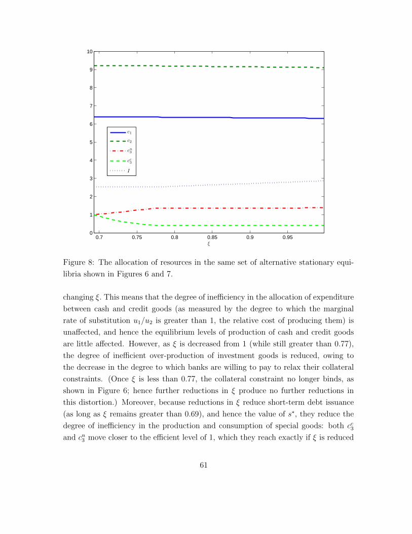
0.7 0.75 0.8 0.85 0.9 0.950

1

2

3

4

5

6

7

8

9

10

ξ

c1

c2

cn3

cc3

I

Figure 8: The allocation of resources in the same set of alternative stationary equi-

libria shown in Figures 6 and 7.

changing ξ. This means that the degree of inefficiency in the allocation of expenditure

between cash and credit goods (as measured by the degree to which the marginal

rate of substitution u1/u2 is greater than 1, the relative cost of producing them) is

unaffected, and hence the equilibrium levels of production of cash and credit goods

are little affected. However, as ξ is decreased from 1 (while still greater than 0.77),

the degree of inefficient over-production of investment goods is reduced, owing to

the decrease in the degree to which banks are willing to pay to relax their collateral

constraints. (Once ξ is less than 0.77, the collateral constraint no longer binds, as

shown in Figure 6; hence further reductions in ξ produce no further reductions in

this distortion.) Moreover, because reductions in ξ reduce short-term debt issuance

(as long as ξ remains greater than 0.69), and hence the value of s∗, they reduce the

degree of inefficiency in the production and consumption of special goods: both cc3and cn3 move closer to the efficient level of 1, which they reach exactly if ξ is reduced

61

to 0.69.

We can now ask to what extent the effects of expanding the supply of central-bank

liabilities through quantitative easing are equivalent, or even similar, to the effects

of relaxing a reserve requirement that limits the ability of banks to issue money-like

liabilities. In the context of our model, the former sort of policy corresponds to an

increase in m (resulting in an increase in Rm/Π, if there is not already satiation in

cash balances), which can be implemented while keeping ξ fixed; the latter sort of

policy corresponds to an increase in ξ (assuming a reserve requirement tight enough

to bind), which can be implemented while keeping m fixed, or with an appropriate

adjustment of the central bank’s balance sheet, while keeping Rm/Π fixed.

A comparison of Figures 6-8 with Figures 2-4 shows that not only are these two

policies not equivalent, their effects are in many respects exactly the opposite. An

expansion of the central bank’s balance sheet while fixing ξ corresponds to a movement

from left to right in Figures 2-4: short-term debt issuance by private banks falls,

both the over-valuation of durables in subperiod 1 and their under-valuation in the

event of a crisis are reduced, the over-production of durables is reduced, and level of

production of special goods in both the c and n states becomes more nearly efficient. A

relaxation of a binding reserve requirement while fixing Rm/Π corresponds instead to

a movement from left to right in Figures 6-8, which essentially reverses the effects seen

in the earlier figures: short-term debt issuance by private banks increases, both the

over-valuation of durables in subperiod 1 and their under-valuation in the crisis state

increase, the over-production of durables in increased, and the level of production of

special goods is progressively more severely distorted.

In fact, both an expansion of the outside supply of safe assets and a tightening

of reserve requirements (or other forms of macroprudential policy) have similar con-

sequences for financial stability, insofar as both reduce the extent to which banks

finance themselves by issuing short-term safe debt. Either of these policies, pur-

sued far enough, will completely eliminate private issuance of money-like claims (the

right boundary of Figures 2-4, or the left boundary of Figures 6-8), and consequently

eliminate the distortions resulting from the risk of a fire sale of assets and from the

desire of bankers to obtain assets that can be used to collateralize short-term debt

issuance. Thus each of these policies, either of which is welfare-enhancing (when

not irrelevant), can serve to some extent as a substitute for the other. It is worth

noting, however, that while a sufficient increase in the outside supply of safe assets

62

would make macroprudential policy unnecessary in our model (since private issuance

of money-like claims can be completely eliminated, even if ξ = 1), the reverse is not

true: even a macroprudential policy of the maximum possible stringency (one that

completely prevents private issuance of STSIs) will not eliminate the welfare gains

from further expansion of the outside supply of safe assets, since even when D = 0

(as in the case with ξ = 0.69 in Figures 6-8), there will still be inefficient under-

consumption of cash goods, owing to the binding cash-in-advance constraint, as long

as m < m∗.

5 Conventional and Unconventional Monetary

Policy in the Presence of Nominal Rigidities

In the analysis thus far, all prices have been assumed to be perfectly flexible, and

to clear markets each period. In such a model, conventional monetary policy has

no real effects, and affects only the general level of prices in terms of the monetary

unit. It follows that conventional monetary policy has no consequences for financial

stability. This establishes a sharp distinction between the effects of conventional

monetary policy (interest-rate policy) and balance-sheet policy, since as shown above,

the central bank’s balance sheet (specifically, the real supply of safe assets by the

central bank) does have consequences for financial stability.

Such an analysis is adequate for consideration of the possible long-run stationary

equilibria achievable under alternative policies, as in the previous two sections. But it

does not suffice for an analysis of the considerations at play when alternative dimen-

sions of monetary policy are used to address short-run macroeconomic stabilization

objectives, and this is the context in which central banks’ recent experiments with

quantitative easing have been conducted. To address the issues raised by recent poli-

cies, we need to consider the consequences for financial stability of using quantitative

easing as a substitute for an interest-rate cut that is prevented by the effective lower

bound on short-term nominal interest rates, in a situation where such an interest-rate

cut would otherwise be desired in order to achieve a higher level of output.

The notion that an interest-rate cut would be desired in order to increase real

activity only makes sense in the presence of nominal rigidities of some kind. Here

we discuss a simple extension of the model presented above, that shows how sticky

63

prices allow conventional monetary policy to have real effects in the short run, while

it affects only the general level of prices in the long run. We can then compare the

effects of quantitative easing to those of an interest-rate cut, both with respect to

the effects of these policies on aggregate demand, and their consequences for financial

stability.

5.1 Equilibrium with a Sticky Price for Normal Goods

We suppose that it is only the price Pt of normal goods that must be set in advance,

while the prices of special goods, durable goods, and all financial assets are assumed to

be perfectly flexible, as above. (Because all three types of normal goods are perfect

substitutes from the standpoint of their suppliers, we suppose that a single price

Pt is posted, at which goods of any of these types can be purchased; we suppose

that the buyer determines which type of good will be obtained.) For simplicity,

we also consider here the case of a single unexpected aggregate shock (apart from

the kind of uncertainty represented in Figure 1) at some date t, in response to which

monetary policy (both interest-rate policy and balance-sheet policy) may be adjusted;

we suppose that there is no further uncertainty (except for the kind depicted in Figure

1) about how the economy will evolve after this shock occurs, and that the shock is

completely unanticipated prior to its occurrence.

The fact that the shock is completely unexpected means that before it occurs,

people expect an equilibrium in which there will never be any random developments

except the kind depicted in Figure 1. We may suppose that this equilibrium is

a stationary equilibrium of the kind described in section 3. Note that in such an

equilibrium, the price Pτ of normal goods in any period τ is a deterministic function

of time; it does not depend on which state is reached in subperiod 2 of period τ , nor

does it depend on the history ξτ of states revealed in previous periods. Hence we

may suppose that the same price Pτ is set for normal goods in all periods τ ≤ t as

would clear markets in the flexible-price stationary equilibrium analyzed above, even

if the price Pτ must be set before subperiod 2 of period τ is reached. For purposes of

the present discussion, we need not discuss how exactly the predetermined price of

normal goods is determined, beyond the assumption that in an environment where

the future is perfectly predictable (except for the uncertainty each period depicted in

Figure 1), the price that is set each period is the one that would clear the market for

64

normal goods.

Let us suppose that period t is one in which no crisis occurs in subperiod 2 (though

it is not known up until this time that this would be the case). But let us also suppose

that in subperiod 2 of period t, an unexpected shock occurs, as a result of which the

utility of cash and credit goods consumption is equal to χu(c1t, c2t), and the disutility

of supplying normal goods is equal to χv(Yt), for some factor χ > 0 that need not

equal 1; the other components of the utility function are unaffected by the shock.

The factor χ is assumed to take a value different from 1 only in period t (and prior

to period t, it is assumed to equal 1 with probability 1 in period t as well). The point

of assuming a shock of this particular type is that for a given level of production

of investment goods, the efficient level of production and consumption of cash and

credit goods would not be changed by the shock χ; however, the real rate of interest

required to sustain that level of demand will change (will be lower if χ is lower).

Hence the shock χ represents a “demand disturbance” to which it would be desirable

to respond by lowering interest rates, if this is not precluded by the interest-rate lower

bound.

Both conventional monetary policy and balance-sheet policy are allowed to re-

spond to the occurrence of the shock, though their paths are assumed to be perfectly

predictable from then on, as with all other exogenous variables. We suppose that Rmτ

and mτ are both determined in subperiod 2 of period τ − 1. Hence neither Rmt nor

mt can be affected by the value of χ; these variables are both equal to their values

in the stationary equilibrium. But Rmτ and mτ can both differ from their stationary

equilibrium values in periods τ ≥ t+ 1.

For simplicity, we shall here consider only policy responses to the shock of a

special sort. We continue to suppose that from period t + 1 onward, conventional

monetary policy (that is, the choice of Rmτ + 1 for all τ ≥ t+ 1) is used to ensure that

the path of normal goods prices {Pτ} grows at the constant rate π∗ in all periods

τ ≥ t + 1.48 We similarly continue to suppose that balance-sheet policy is used to

48Note that Pt+1 is set in advance on the basis of expectations about the demand for normal

goods in period t+ 1, which will depend on the interest rate Rmt+2 because of condition (2.15). Thus

the rule for setting Rmτ+1 in periods τ ≥ t+ 1 can be used to ensure that the market-clearing price

for normal goods in all periods τ ≥ t+ 1 are consistent with the inflation target. This desideratum

leaves the value of Rmt+1 undetermined. Note that the value of Pt reflects expectations about how

Rmt+1 would be set; but these are expectations about monetary policy in period t that were held

prior to the unexpected shock, that may not be confirmed, as a result of the shock.

65

achieve a real outside supply of cash mτ+1 equal to the stationary equilibrium value

m for all τ ≥ t+ 1. We can then reduce the set of alternative monetary policies that

we consider to a two-parameter family, corresponding to different possible choices of

Rmt+1 and mt+1 (both of which must be chosen in subperiod 2 of period t, but which

may depend on the value of χ).49

Because the price Pt has been fixed in advance, it is assumed to be independent

of the value of χ, and equal to the price associated with the stationary equilibrium

that had previously been expected to continue. Once the shock χ occurs, there is

no further uncertainty about how the economy will evolve from then on (except the

uncertainty depicted in Figure 1). Hence we may suppose that the price Pτ of normal

goods in each period τ ≥ t + 1 is set so as to clear the market for normal goods in

that period. (While we assume that Pτ must be set prior to subperiod 2 of period

τ , we suppose that it is not set prior to subperiod 2 of period τ − 1.50) Thus in the

equilibrium considered in this section, the only period in which the market for normal

goods need not clear is period t (the period in which the shock χ occurs); in that

period, Pt is set at the level that would clear the market in the event that χ = 1.

More generally, we shall suppose that all variables that are determined in sub-

period 1 of period t, or earlier, are determined in the way that they are in the

equilibrium in which χ = 1 is expected (that is, as in the stationary equilibrium with

flexible prices implied by the initial policy). Thus the values of At,Mt, Bt, Dt, Ft, st,

and Qt are unaffected by the shock, in addition to Pt and all variables dated t − 1

or earlier. Instead the variables c1t, c2t, c3t, It, Yt, xt, and Pt, as well as all variables

dated t+ 1 or later, are determined in a way that takes account of the occurrence of

the shock χ.51 The Lagrange multipliers ϕ4t, ϕ5t, and ϕ6t are jointly determined with

this latter set of variables (as well as the Lagrange multipliers for later periods).

The variables that are affected by the shock χ are determined by a system of

intertemporal equilibrium conditions of the form stated earlier, with the following

49For simplicity, in this section we abstract from the possible use of macroprudential policy, as in

sections 1-3; that is, we consider only equilibria in which ξt = 1 at all times.50This means that the length of time for which prices are sticky is limited in the proposed model.

A quantitatively realistic model would doubtless need to allow some prices to remain fixed for a

longer period, but the simple case considered here suffices to illustrate the qualitative effects of

temporary stickiness of prices.51Note that the variables s∗t and Γt are undefined, as we have assumed that the crisis state does

not occur in period t.

66

exceptions. First, the fact that the suppliers of normal goods must supply whatever

quantity of such goods is demanded at the predetermined price Pt means that the

FOC (2.13) need not be satisfied in period t ex post (that is, after the shock χ occurs).

However, the other FOCs for optimal household behavior stated above continue to

apply, and (2.13) also must hold in periods t+ 1 and later (since normal goods prices

in those periods are set in a way that clears the market). Thus we drop one (but only

one) of the conditions that would determine a flexible-price intertemporal equilibrium

from subperiod 2 of period t onward, replacing it by the requirement that Pt equal a

predetermined value, whether this clears the market for normal goods or not. Second,

the partial derivatives ui(c1, c2) in FOCs (2.9)–(2.10) are replaced by χui(c1, c2) (for

i = 1, 2) in period t only. All other FOCs and market-clearing conditions continue to

take the forms stated above.

The demand for cash and credit goods in period t will then be given by

c1t = c1(λt/χ;Mt/Pt), c2t = c2(λt/χ;Mt/Pt),

where Mt/Pt is unaffected by the shock. Aggregate demand for normal goods in

period t is accordingly

Yt = c1(λt/χ;Mt/Pt) + c2(λt/χ;Mt/Pt) + I(λt;λt+1, mt+1). (5.1)

Since c1(λ;m) and c2(λ;m) are both non-increasing functions of λ, and at least c2

must be decreasing, it follows that aggregate demand is a monotonically increasing

function of χ, for given values of λt and λt+1.

Condition (2.40) continues to be a requirement for equilibrium, as a result of

which we must have

λt = β λt+1 ϕ1(λt+1;F (I(λt;λt+1, mt+1)), mt+1)Rmt+1

PtPt+1

. (5.2)

This equation indicates the way in which the choice of Rmt+1 in period t affects the value

of λt, and through it aggregate demand Yt, for given expectations about conditions

in period t + 1. Note that if the price Pt were required to clear the market for

normal goods, substitution of (5.1) into (2.13) would yield a condition to determine

the required value of λt in equilibrium; (5.2) would then indicate the interest rate

Rmt+1 required to achieve the price-level target Pt. Under the assumption that Pt is

predetermined and need not clear the market, it is possible for Rmt+1 to change in

67

response to the shock, resulting in a value of Yt that need not satisfy the voluntary

supply condition (2.13).

In each period from t + 1 onward, we effectively have flexible prices, so that

condition (2.39) is again required for equilibrium. Thus for any specification of Rmt+1

and of the path {mτ} for all τ ≥ t + 1, the equilibrium sequence {λτ} for τ ≥ t is

determined by condition (5.2) and the sequence of conditions of the form (2.39) for

each period from t + 1 onward. Given a solution for the sequence {λτ}, aggregate

demand for normal goods is determined by (5.1) in period t, and by (2.37) in each

period from t+ 1 onward. The implied equilibrium values of other variables are then

determined in the way discussed in section 2.

5.2 Real Effects of Conventional and Unconventional

Monetary Policy

We can now compare the effects of quantitative easing with those of conventional

interest-rate policy, as possible responses to a shock χ. Note that if both Rmt+1 and

the path {mτ} for t ≥ t+ 1 remain fixed at the values associated with the stationary

equilibrium in which there is no shock, then the values λτ = λ for all τ ≥ t will satisfy

condition (2.39) in period t and condition (2.39) for each of the periods t+1 and later,

where λ is the constant value of λτ in the stationary equilibrium. Aggregate demand

for normal goods in period t is then given by (5.1). If χ = 0, this implies Yt = Y , the

constant level of output in the stationary equilibrium. If instead χ < 0, we will have

Yt < Y . This reduction in the production of normal goods will be inefficient, since it

will imply that

u2(c1t, c2t) = χλ < λ = v′(Y ) ≤ v′(Yt),

so that the marginal utility of additional consumption of normal goods would exceed

the marginal disutility of supplying them.

We consider now the extent to which monetary policy can be used to respond to

such a shock. In addition to the effects of policy on production and consumption,

we shall be interested in how each of our possible dimensions of central-bank policy

influence financial conditions. Two measures of financial conditions are especially

useful. One is the size of the money premium earned by cash, which we can measure

68

by the extent to which the ratio

Et[Rbt+1]

Rmt+1

= ϕ1,t+1

is greater than one. This is a measure of financial conditions that determines the

incentives for short-term debt issuance by banks. Another important measure is the

expected one-period real return on longer-term bonds,

1 + rbt+1 ≡ Et+1

[Rbt+1PtPt+1

]=

λtβλ

.

(Note that this aspect of financial conditions can alternatively be measured by the

value of λt.) This is the measure of financial conditions that is relevant for determining

the aggregate demand for non-durable normal goods, as a result of (5.1). Below we

analyze the effects of each of the dimensions of policy on both of these measures of

financial conditions.

5.2.1 Conventional Monetary Policy

Conventional monetary policy can be used to mitigate the effects of a χ shock by

lowering Rmt (if this is not prevented by the lower bound on the nominal interest

rate). The effects of such policy are most easily seen in the special case that v(Y )

is linear, so that v′(Y ) = λ regardless of the value of Y . Then (2.39) requires that

λt+1 = λ, and (5.2) reduces to

λt = β λ ϕ1(λ;F (It), mt+1)Rmt+1/Π. (5.3)

Here we have also substituted the target gross inflation rate Π for Pt+1/Pt, on the

assumption that interest-rate policy in period t+ 1 is used to ensure that the target

inflation rate is realized, regardless of other conditions.

For simplicity, we discuss here only the case of an equilibrium in which bankers’

collateral constraint binds in period t+1, so that durables are over-valued in subperiod

1. (Note that this is the case in which risks to financial stability are of the greatest

concern.) In this case, we can use

Mt/Pt = mt + λ−1t Γ(st)st

69

(which follows from (2.29)), together with the fact that ϕ1(λ;m) is decreasing in both

arguments (as shown in section 2), to conclude that ϕ1(λ; s, m) will be a decreasing

function of both s and m, for any fixed value of λ.

In addition, (2.35) requires that

λt = β φ(λ;F (It), mt+1)F′(It). (5.4)

This establishes an equilibrium relationship between investment demand It and fi-

nancial conditions as measured by λt (though it is important to note that the value

of mt+1 remains of independent relevance). Equating the right-hand sides of (5.3)

and (5.4), we see that equilibrium investment It must satisfy

ϕ1(λ;F (It), mt+1) =Π

λ Rmt+1

φ(λ;F (It), mt+1)F′(It). (5.5)

Again restricting attention to the case where bankers’ collateral constraint binds

in period t + 1, we can alternatively express the function φ(λ; s, m) in terms of the

function ϕ1. Note that

ϕ1tQt = Q∗ + (1− p)ϕ3t Γt

= Q∗ + (1− p)[(ϕ2t + 1) Γt − γq]

= γp) + [ϕ1t − p] Γt,

using (2.5), (2.6), and (2.4) in succession. It follows that we can express the function

φ as

φ(λ; s, m) ≡ φ(ϕ1(λ; s, m); s), (5.6)

where

φ(ϕ1; s) ≡ γp + [ϕ1 − p] Γ(s). (5.7)

Condition (5.5) can then be written alternatively in the form

ϕ1,t+1 =Π

λ Rmt+1

φ(ϕ1,t+1;F (It))F′(It) (5.8)

using (5.6). This describes a relationship that must exist between investment demand

It and the money premium ϕ1,t+1 in the case of any given specification of conven-

tional monetary policy. It is worth noting (for the sake of our discussion below of

quantitative easing) that this relationship is unaffected by the value of mt+1.

70

Because Γ(s) ≤ γq < γ, (5.7) implies that

0 <∂φ

∂ϕ1

<φ

ϕ1

,∂φ

∂s< 0.

It follows from these that (5.8) implicitly defines a function

ϕ1,t+1 = ϕ1(It, Rmt+1) (5.9)

which is decreasing in both arguments.

Using this together with (2.34), we see that the equilibrium level of investment It

must satisfy

ϕ1(λ;F (It), mt+1) = ϕ1(It, Rmt+1). (5.10)

This can be solved for the effects of monetary policy on investment. Given that

ϕ1(λ; s,m) is a decreasing function of s (when the collateral constraint binds), we see

that both sides of (5.10) are decreasing functions of It.

The comparative statics of It in response to a change in either Rmt+1 or mt+1 then

depend on the relative slopes of these two schedules. We shall assume that in the

initial equilibrium, relative to which we wish to consider the effects of a change in

monetary policy,∂ϕ1

∂I<

∂ϕ1

∂I< 0, (5.11)

as shown in the upper part of Figure 9. In this case we obtain the conventional signs

for the short-run effects of interest-rate policy.52 In particular, because ϕ1(I, Rm) is a

decreasing function of Rm, a reduction of Rmt+1 will increase It, as shown in the figure.

It also follows from (5.6) and the fact that ϕ1(λ; s,m) is a decreasing function of

s that φ(λ; s, m) is also a decreasing function of s. Thus the right-hand side of (5.4)

is a decreasing function of It, for any fixed value of mt+1. Hence (5.4) establishes an

inverse relationship between λt and It that must hold regardless of the value chosen

52Note that if the inequality (5.11) is reversed, our model would imply that a reduction in the

interest rate on cash is associated with a decrease, rather than an increase, in aggregate demand.

Condition (5.4) establishes an inverse relationship between λt and It, regardless of whether (5.11)

holds; so if a reduction of Rmt+1 were associated with a reduction of It, this would have to mean

an increase in λt, and hence a decrease in all three terms on the right-hand side of (5.1). Such an

effect would be contrary to familiar evidence regarding the effects of interest-rate policy, and would

also preclude the possibility of a “liquidity trap” in which the lower bound on nominal interest rates

prevents rates from being cut enough to maintain a desired level of real activity.

71

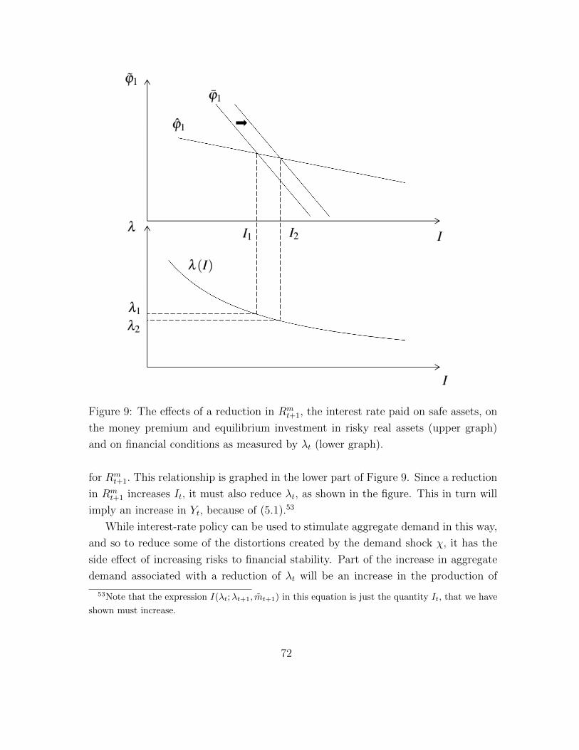
Figure 9: The effects of a reduction in Rmt+1, the interest rate paid on safe assets, on

the money premium and equilibrium investment in risky real assets (upper graph)

and on financial conditions as measured by λt (lower graph).

for Rmt+1. This relationship is graphed in the lower part of Figure 9. Since a reduction

in Rmt+1 increases It, it must also reduce λt, as shown in the figure. This in turn will

imply an increase in Yt, because of (5.1).53

While interest-rate policy can be used to stimulate aggregate demand in this way,

and so to reduce some of the distortions created by the demand shock χ, it has the

side effect of increasing risks to financial stability. Part of the increase in aggregate

demand associated with a reduction of λt will be an increase in the production of

53Note that the expression I(λt;λt+1, mt+1) in this equation is just the quantity It, that we have

shown must increase.

72

investment goods, as a result of which st+1 will be higher. In the case of an equilibrium

in which the collateral constraint binds, this will mean a correspondingly higher value

of s∗t+1, as a consequence of which the degree of under-valuation of durables in the

event of a crisis and fire sale will be more severe. Thus in the sticky-price version

of the model, it is indeed the case that reducing short-term nominal interest rates

increases risk-taking by banks in a way that makes the distortions associated with a

crisis more severe, should one occur.

5.2.2 Effects of Unconventional Policies

In the event that the lower bound on interest rates prevents Rmt+1 from being reduced

to the extent that would be necessary to maintain aggregate demand at the desired

level, quantitative easing provides an alternative channel through which aggregate

demand may be increased. Like conventional interest-rate policy, an expansion of

the supply of short-term safe assets by the central bank affects aggregate demand by

easing financial conditions, as indicated by a reduction in λt (which can be thought

of as the price of a particular very-long-duration indexed bond).

Consider the effects of an increase in mt+1, holding Rmt+1 fixed. We can again

determine the effect on equilibrium investment demand using (5.10). The schedule

corresponding to the right-hand side of this equation does not shift as a result of an

increase in mt+1, but the fact that ϕ1(λ; s, m) is a decreasing function of m means

that the schedule corresponding to the left-hand side of the equation shifts down for

each possible value of It, as shown now in the upper part of Figure 10. Then again

assuming that the relative slopes of the two schedules are given by (5.11), we can

again conclude that It must increase while ϕ1,t+1 must decrease.

We can also again use (5.4) to determine the change in λt required by a given

size increase in It. As argued above, an increase in It reduces the right-hand side

of this equation, for any given value of mt+1. In addition, (5.6) together with the

result above that ϕ1(λ; s, m) is a decreasing function of m implies that the function

φ(λ; s, m) is also a decreasing function of m. This means that the curve (the graph

of equation (5.4)) graphed in the lower part of Figure 10 shifts down as a result of

an increase in mt+1, as shown in the figure. It then follows that λt is reduced by an

increase in mt+1, both because of the decrease in It (the shift along the curve) and

because of the direct effect of an increase in mt+1 (the downward shift of the curve).

It follows that an increase in mt+1 must loosen financial conditions, in the sense

73

Figure 10: The effects of an increase in the central-bank supply of safe liabilities mt+1

on the money premium and equilibrium investment in risky real assets (upper graph)

and on financial conditions as measured by λt (lower graph).

that λt is reduced. This in turn means that, as in the case of an interest-rate cut, Yt

must increase because of (5.1). Thus the effects of quantitative easing are qualitatively

similar to those of an interest-rate cut: financial conditions are eased, the aggregate

demand for normal goods increases (both because of an increase in the demand for

credit goods and an increase in the demand for investment goods), but at the same

time risks to financial stability increase, because of an increase in short-term debt

issuance by banks, leading to larger expected distortions in the case that a crisis state

occurs in period t+ 1.

Nonetheless, the two policies do not have quantitatively equivalent effects. If we

74

compare an interest-rate cut (reduction in Rmt+1) and an increase in the net supply

of safe assets by the central bank (increase in mt+1) that increase the equilibrium

demand for investment goods It by the same amount, the increase in mt+1 reduces λt

by a greater amount.54 This can be seen from the fact that (5.4) must apply in either

case. If, by hypothesis, It increases by the same amount in both cases, then the only

difference in the implied value for λt is that mt+1 increases in the second case, but

remains constant in the first; and this implies a lower value of λt in the second case.

This means that in the case of quantitative easing, a greater share of the total increase

in aggregate demand comes from increased demand for credit goods, as opposed to

increased demand for investment goods. Thus a given degree of aggregate demand

stimulus can be achieved with less risk to financial stability if it is brought about

through an expansion of the central bank’s balance sheet, rather than by cutting the

interest rate paid on cash.

We can also consider the effects of aggregate demand stimulus through relaxation

of macroprudential constraints (that is, an increase in ξt+1). Let us generalize the

analysis presented in the earlier part of this section to allow for a macroprudential

tax (or reserve requirement), so that ξt need not equal 1 (as assumed thus far in this

section). Conditions (5.1), (5.3) and (5.4) continue to be required for an equilibrium,

and the definition of the function ϕ1(λ; s, m) is unchanged; but in (5.4), the expression

φ(λ;F (It), mt+1) must be replaced by φ(λ;F (It), mt+1, ξt+1), where we define

φ(λ; s, m, ξ) ≡ φ(ξϕ1(λ; s, m); s),

generalizing (5.6).

Condition (5.8) then takes the more general form

ϕ1,t+1 =Π

λ Rmt+1

φ(ξt+1ϕ1,t+1;F (It))F′(It).

As above, this implicitly defines a function

ϕ1,t+1 = ϕ1(It, Rmt+1, ξt+1), (5.12)

where now ϕ1(I, Rm, ξ) is decreasing in I and Rm, and increasing in ξ. The equilib-

rium level of investment is again determined by (5.10), but now the schedule corre-

54Compare Figures 9 and 10. In Figure 10, the amount of quantitative easing is chosen so as to

achieve the same increase in investment (from I1 to I2) as the interest-rate cut in Figure 9. The

reduction in λt is instead larger (from λ1 to λ3 < λ2).

75

sponding to the left-hand side is shifted only by mt+1, while the schedule correspond-

ing to the right-hand side is shifted by changes in either Rmt+1 or ξt+1. To a linear

approximation (which is to say, in the case of small enough policy changes), then, an

increase in ξt+1 (a relaxation of macroprudential policy, as by reducing the required

reserve ratio) has the same effects on It and ϕ1,t+1 as a certain size of cut in Rmt+1.

We can also use (5.12) to rewrite (5.3) in the form

λt = β λ ϕ1(It, Rmt+1, ξt+1)R

mt+1/Π. (5.13)

From this it follows that since a relaxation of macroprudential policy reduces the value

of ϕ1,t+1, it must reduce the value of λt. Hence it increases demand for credit goods,

and so must increase Yt, like the other two policies just considered. But it also follows

from (5.13) that in the case of two policy changes (a cut in Rmt+1 or an increase in ξt+1)

that reduce ϕ1,t+1 to the same extent, and that therefore reduce ϕ1(It, Rmt+1, ξt+1) to

the same extent, the interest-rate cut must reduce λt by more, and so must stimulate

demand for credit goods to a greater extent. Thus an even greater share of the

increase in aggregate demand achieved by relaxing macroprudential policy comes

from an increase in investment demand, as opposed to an increase in the demand for

credit goods, than in the case of an increase in aggregate demand achieved by cutting

the interest rate on cash.

We can therefore order the three types of expansionary policy: for a given degree

of increase in aggregate demand, achieving it by increasing mt+1 increases It the least,

achieving it by reducing Rmt+1 increases It to an intermediate extent, and achieving

it by increasing ξt+1 increases It (and hence short-term debt issuance by banks, and

risks to financial stability) the most. One consequence of this is that increasing

aggregate demand through monetary policy need not involve any increased risks to

financial stability at all. For example, one might combine an increase in mt+1 with

a tightening of macroprudential policy (reduction of ξt+1) that exactly offsets the

effects of the quantitative easing on desired investment demand, so that there is no

net change in It. Since the former policy change will reduce λt more than the latter

policy change increases it, the net effect will be a loosening of financial conditions,

and an increase in the demand for credit goods. Since there is (by hypothesis) no

change in investment demand, aggregate demand Yt will increase; but there will be

no associated increase in st+1, and hence no increase in the severity of the distortions

associated with a crisis state in period t+ 1.

76

We conclude that while quantitative easing may increase risks to financial stabil-

ity in the case that nominal rigidities allow short-run effects of monetary policy on

aggregate demand, it need not have any such effect. If the increase in the central

bank’s balance sheet is combined with an increase in the interest rate paid on cash, or

a tightening of macroprudential policy to a sufficient extent, it can increase aggregate

demand without any adverse consequences for financial stability. It is particularly

easy to achieve this outcome by combining the quantitative easing with macropruden-

tial policy, if a suitable macroprudential instrument exists; for in our model, reduction

of ξt+1 provides an even greater disincentive to issuance of short-term debt by banks

than does raising Rmt+1, for a given degree of reduction in aggregate demand.

These results imply that quantitative easing may be a useful addition to a central

bank’s monetary policy toolkit, even when interest-rate policy is not yet constrained

by the effective lower bound on short-term nominal interest rates. In the case of a

contractionary shock χ, the effects on aggregate demand can be offset purely through

a reduction in Rmt+1, if the lower bound does not prevent the size of rate cut that

is needed; but such a response increases risks to financial stability more than is

necessary. One could alternatively counter the effects of the χ shock by increasing

mt+1, while leaving Rmt+1 unchanged; and this would have the advantage of posing less

of a threat to financial stability. Even better, one could combine a somewhat larger

increase in mt+1 with a tightening of macroprudential policy, allowing the effects of

the χ shock on aggregate demand to be offset, with even less of an increased risk to

financial stability, possibly none at all.

6 Conclusions

We can now assess the validity of the concerns about the consequences of quantitative

easing for financial stability sketched in the introduction, in the light of the model

just presented. Our model is one in which monetary policy does indeed influence risks

to financial stability; in particular, policies that loosen financial conditions, either by

lowering the central bank’s operating target for its policy rate (conventional monetary

policy), or by relaxing reserve requirements (or other macro-prudential constraints),

should each increase the attractiveness of private issuance of “money-like” liabilities,

resulting in increased leverage and as a consequence an increased risk of serious

resource misallocation in the event of a funding crisis. This means that there can

77

at times be a tension between the monetary policy that would be preferable strictly

from the standpoint of aggregate demand management and inflation stabilization, on

the one hand, and the policy that would minimize risks to financial stability.

The question is whether it is correct to think of quantitative easing as a policy

analogous to these, and hence that poses similar risks to financial stability. Our model

implies that such an analogy is imperfect. A quantitative easing policy (increasing the

public supply of safe assets, by issuing additional safe liabilities of the central bank,

used to purchase assets that do not earn a similar safety premium) similarly increases

aggregate demand by lowering the equilibrium rate of return on non-safe assets. But

unlike conventional monetary policy, it does this by lowering the equilibrium safety

premium (by making safe assets less scarce), rather than by lowering the equilibrium

return on safe assets; and this does not have the same consequences for financial

stability. Lowering the equilibrium return on risky investments (such as the “durable

goods” modeled here, which one may think of as housing) by lowering the return on

safe assets works only insofar as the increased spread between the two returns that

would result if the return on risky investments did not also fall increases the incentive

to finance additional risky investment by issuing safe liabilities, thus increasing the

leverage of the banks and the degree to which they engage in liquidity transformation;

this results in a reduced equilibrium return on risky investment, but not by enough

to fully eliminate the increased spread that induces banks to issue additional safe

asset-backed liabilities. This mechanism necessarily increases the risk to financial

stability at the same time as it increases aggregate demand. Quantitative easing

instead decreases the spread between these two returns, at least in the absence of

any change in the private supply of safe liabilities. This reduction in the spread

reduces the incentive for private issuance of such liabilities, and reduced issuance of

safe asset-backed liabilities by banks offsets some of the reduction in the spread, but

does not completely eliminate it as otherwise banks would not have a reason to reduce

their issuance. Hence in this case the reduction in the equilibrium return on risky

investments is associated with a reduction of the incentive for liquidity transformation

by banks, rather than an increase.

Similarly, quantitative easing increases the total supply of safe assets and so re-

duces the safety premium; but unlike a reduction in reserve requirements (or relax-

ation of macroprudential policy), it achieves this by increasing the public supply of

safe assets (and actually reducing the incentive for private issuance), rather than by

78

increasing the incentive that banks have to finance risky investment by issuing safe

asset-backed liabilities. Again the consequences for the degree of liquidity transfor-

mation by the banking sector, and hence the risk to financial stability, are entirely

different.

Likewise, it is true that quantitative easing eases financial conditions by reducing

the spread between the required return on risky investments and the return on safe

assets; but this does not mean that risk premia are “artificially” reduced in a way that

distorts incentives for prudent behavior, leading to excessive risk-taking. In the model

presented here, quantitative easing reduces the safety premium, but because the pub-

lic supply of safe assets for private investors to hold is increased, and not because

anyone is misled into under-estimating the degree of risk involved in undertaking

risky investments. Moreover, the reduced spread reduces the incentive for private is-

suance of safe liabilities, and instead favors financing of investment through issuance

of non-safe liabilities, which is desirable on financial stability grounds. Rather than

threatening financial stability by encouraging more risk-taking, it favors it by encour-

aging forms of financing that reduce the magnitude of the distortions associated with

a funding crisis.

In our model, we can compare the effects of three alternative policies that can in-

crease aggregate demand by easing financial conditions: reducing the central bank’s

operating target for the nominal interest rate on safe assets (conventional monetary

policy, on the assumption that the zero lower bound does not yet preclude such

easing), relaxing reserve requirements (or other macro-prudential constraints), and

quantitative easing. We find that among these, quantitative easing is the policy that

increases risks to financial stability the least, for any given degree of increase in aggre-

gate demand. Not only does quantitative easing make it possible for a central bank

to increase aggregate demand even when conventional monetary policy is constrained

by the zero lower bound on nominal interest rates, but it is possible, at least in prin-

ciple, to increase aggregate demand without the collateral effect of an increased risk

to financial stability, if the increased supply of safe liabilities by the central bank

is combined with a sufficient tightening of macroprudential measures. (The latter

measures would by themselves reduce aggregate demand; but when combined with

quantitative easing, the net effect is an increase in aggregate demand, even when the

degree of macroprudential tightening is enough to fully offset any increase in risks to

financial stability as a result of the balance-sheet policy.)

79

This indicates that a concern for the effects of monetary policy on financial sta-

bility need not preclude using quantitative easing to stimulate aggregate demand in

circumstances where (as in the US in the aftermath of the recent crisis) conventional

monetary policy is constrained by the zero lower bound. In fact, the fact that de-

mand stimulus through quantitative easing poses smaller risks to financial stability

than demand stimulus through lowering short-term nominal interest rates suggests

that balance-sheet policy may be a useful tool of monetary stabilization policy even

when a central bank is far from the zero lower bound. In the model presented here,

aggregate demand stimulus achieved by lowering nominal interest rates increases the

risk to financial stability more than would a quantitative easing policy that is equally

effective in increasing aggregate demand. This implies that (even if macropruden-

tial policy is unavailable or ineffective) it should be possible to increase aggregate

demand without increasing the risk to financial stability by combining expansionary

balance-sheet policy with an appropriate size of increase in the policy rate. In such

a case, conventional monetary policy would essentially be used for macroprudential

purposes (to control the risk to financial stability) while balance-sheet policy is used

for demand stabilization.

Further study of the effects of quantitative easing policies would therefore seem to

be warranted, not simply for the sake of having a more effective policy toolkit for use

the next time that conventional policy is again constrained by the zero lower bound,

but also, arguably, in order to improve the conduct of stabilization policy under

more normal circumstances as well. The availability of this additional dimension

of monetary policy is particularly likely to be of use under circumstances where

additional monetary stimulus through interest-rate reduction is unattractive owing

to concerns about financial stability. Such a situation could easily arise even when

interest rates are well above their effective lower bound.

80

References

[1] Adrian, Tobias, and Hyun Song Shin, “Financial Intermediaries and Monetary

Economics,” Handbook of Monetary Economics, vol. 3A, Amsterdam: Elsevier

Press, 2010.

[2] Bernanke, Ben S., “Opening Remarks: Monetary Policy Since the Onset of the

Crisis,” in The Changing Policy Landscape, Kansas City: Federal Reserve Bank

of Kansas City, 2012.

[3] Brunnermeier, Markus K., “Deciphering the Liquidity and Credit Crunch 2007-

2008,” Journal of Economic Perspectives, 23(1): 77-100 (Winter 2009).

[4] Brunnermeier, Markus K., and Lasse Heje Pederson, “Market Liquidity and

Funding Liquidity,” Review of Financial Studies 22: 2201-2238 (2009).

[5] Caballero, Ricardo J., and Emmanuel Farhi, “A Model of the Safe Asset Mech-

anism (SAM): Safety Traps and Economic Policy,” NBER Working Paper no.

18737, January 2013.

[6] Carlson, Mark, Burcu Duygan-Bump, Fabio Natalucci, William R. Nelson,

Marcelo Ochoa, Jeremy Stein, and Skander Van den Heuvel, “The Demand for

Short-Term Safe Assets and Financial Stability: Some Evidence and Implications

for Central Bank Policies,” FEDS paper no. 2014-102, Federal Reserve Board,

November 25, 2014.

[7] Eggertsson, Gauti B., and Michael Woodford, “The Zero Bound on Interest

Rates and Optimal Monetary Policy,” Brookings Papers on Economic Activity

2003-1, pp. 139-211.

[8] Giavazzi, Francesco, and Alberto Giovannini, “Central Banks and the Financial

System,” in S. Eijffinger and D. Masciandaro, eds., Central Banking, Financial

Regulation and Supervision After the Financial Crisis, Cheltenham, UK: Edward

Elgar, 2012.

[9] Gorton, Gary, Slapped by the Invisible Hand: The Panic of 2007, Oxford: Oxford

University Press, 2010.

81

[10] Gorton, Gary, and George Pennacchi, “Financial Intermediaries and Liquidity

Creation,” Journal of Finance 45: 49-71 (1990).

[11] Gorton, Gary, Stefan Lewellen, and Andrew Metrick, “The Safe-Asset Share,”

American Economic Review 102(3): 101-106 (2012).

[12] Greenwood, Robin, Samuel G. Hanson, Joshua S. Rudolph, and Lawrence H.

Summers, “Government Debt Management at the Zero Lower Bound,” Hutchins

Center Working Paper no. 5, September 30, 2014.

[13] Greenwood, Robin, Samuel G. Hanson, and Jeremy C. Stein, “A Gap-Filling

Theory of Corporate Debt Maturity Choice,” Journal of Finance 65: 993-1028

(2010).

[14] Jeanne, Olivier, and Anton Korinek, “Managing Credit Booms and Busts: A

Pigouvian Taxation Approach,” NBER Working Paper no. 16377, September

2010.

[15] Krishnamurthy, Arvind, and Annette Vissing-Jorgensen, “The Aggregate De-

mand for Treasury Debt,” Journal of Political Economy 120: 233-267 (2012).

[16] Krugman, Paul R., “It’s Baaack: Japan’s Slump and the Return of the Liquidity

Trap,” Brookings Papers on Economic Activity 1998-2, pp. 137-206.

[17] Lorenzoni, Guido, “Inefficient Credit Booms,” Review of Economic Studies 75:

809-833 (2008).

[18] Lucas, Robert E., Jr., and Nancy L. Stokey, “Money and Interest in a Cash-in-

Advance Economy,” Econometrica 55: 491-513 (1987).

[19] Sergeyev, Dmitriy, “Optimal Macroprudential and Monetary Policy in a Cur-

rency Union,” working paper, Universita Bocconi, March 2016.

[20] Shleifer, Andrei, and Robert W. Vishny, “Liquidation Values and Debt Capacity:

A Market Equilibrium Approach,” Journal of Finance 47: 1343-1366 (1992).

[21] Shleifer, Andrei, and Robert W. Vishny, “Fire Sales in Finance and Macroeco-

nomics,” Journal of Economic Perspectives, 25(1): 29-48 (Winter 2011).

82

[22] Stein, Jeremy C., “Monetary Policy as Financial-Stability Regulation,” Quar-

terly Journal of Economics 127: 57-95 (2012).

[23] Woodford, Michael, Interest and Prices: Foundations of a Theory of Monetary

Policy, Princeton: Princeton University Press, 2003.

83