Quantitative Biology Lecture 2

(probability distributions + diffusion)

Gurinder Singh “Mickey” Atwal Center for Quantitative Biology

22nd Sep 2015

Summary  

•  Probability  distribu0ons  in  biology    •  Delbruck-­‐Luria  Experiment  

•  Central  Limit  Theorem    •  Molecular  Diffusion  

Probability  and  Sta0s0cs  in  Biology  

 MODELS  •  Molecular  biology  is  fundamentally  noisy  and  processes  are  best  described  probabilis)cally.  

 DATA  ANALYSIS  •  Interpreta0on  of  finite  noisy  measurements  

Sequence  Analysis  •  CAGCCAGACTGCCTTCCGGGTCACTGCCATGGAGGAGCCGCAGTCAGATCCTAGCGTCGAGCCCCCTCTGA

GTCAGGAAACATTTTCAGACCTATGGAAACTGTGAGTGGATCCATTGGAAGGGCAGGCCACCACCCCGACCCCAACCCCAGCCCCCTAGCAGAGACCTGTGGGAAGCGAAAATTCATGGGACTGACTTTCTGCTCTTGTCTTTCAGACTTCCTGAAAACAACGTTCTGGTAAGGACAAGGGTTGGGCTGGGACCTGGAGGGCTGGGGGGGCTGGGGGGCTGGGACCTGGTCCTCTGACTGCTCTTTTCACCCATCTACAGTCCCCCTTGCCGTCCCAAGCAATGGATGATTTGATGCTGTCCCCGGACGATATTGAACAATGGTTCACTGAAGACCCAGGTCCAGATGAAGCTCCCAGAATGCCAGAGGCTGCTCCCCGCGTGGCCCCTGCACCAGCAGCTCCTACACCGGCGGCCCCTGCACCAGCCCCCTCCTGGCCCCTGTCATCTTCTGTCCCTTCCCAGAAAACCTACCAGGGCAGCTACGGTTTCCGTCTGGGCTTCTTGCATTCTGGGACAGCCAAGTCTGTGACTTGCACG  

Biological  Problem  Given  this  sequence  :  • how  do  we  quan0fy  this  sequence?  • can  we  determine  what  organism  this  sequence  comes  from?  • is  the  sequence  different  from  the  rest  of  the  genome?  

Sequence  taken  from  TP53  gene  

Solu0on    Probabilis0c  model  (sta0s0cs)  

Binomial  Distribu0on  

•  Example:  what  is  the  probability  of  observing  n  guanine  bases  in  a  genomic  segment  of  size  L  bases?  

P (n) =L!

(L− n)!n!pn(1− p)L−n

�Ln

�≡ L!

(L− n)!n!shorthand  nota0on  

p  =  probability  of  G  base  

q ≡ 1− p

Permuta0ons    

(understanding  the  L!/(L-­‐n)!n!  prefactor  in  the  binomial  distribu0on)  

 

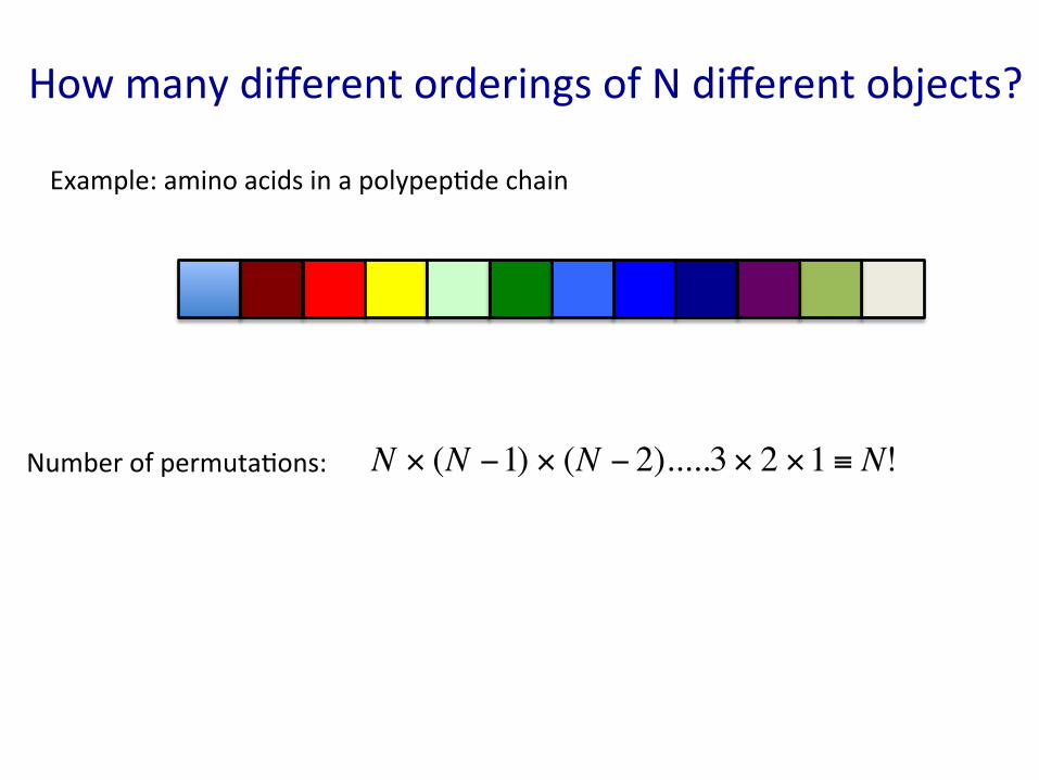
How  many  different  orderings  of  N  different  objects?  

!

N " (N #1) " (N # 2).....3 " 2 "1 $ N!

Example:  amino  acids  in  a  polypep0de  chain  

Number  of  permuta0ons:  

How  many  different  orderings  of  N  different  objects?  

!

N!3!

*   *   *  

3  objects  are  iden0cal  

Number  of  permuta0ons:  

How  many  different  orderings  of  N  objects?  

!

N!R!(N " R)!

#NR$

% & '

( )

R  red  objects  B=(N-­‐R)  blue  objects  

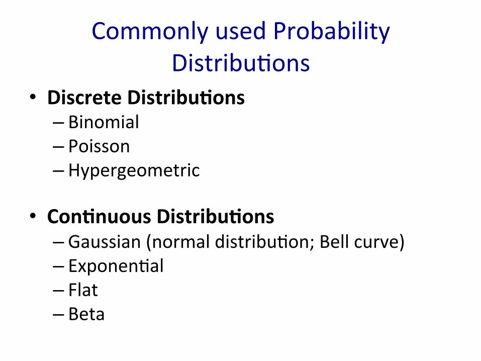
Commonly  used  Probability  Distribu0ons  

•  Discrete  Distribu0ons  – Binomial  – Poisson  – Hypergeometric  

•  Con0nuous  Distribu0ons  – Gaussian  (normal  distribu0on;  Bell  curve)  – Exponen0al  – Flat  – Beta  

Proper0es  of  binomial  distribu0on  

!

P(n;N, p) =Nn"

# $ %

& ' pn (1( p)N (n

!

n = nP(n;N, p) = Npn=0

N

"

!

"2 = n # n( )2

= Np(1# p)

MEAN  

VARIANCE  

Probability  of  k  events  occurring  out  of  n  chances,  with  each  event  occurring  with  probability  p  

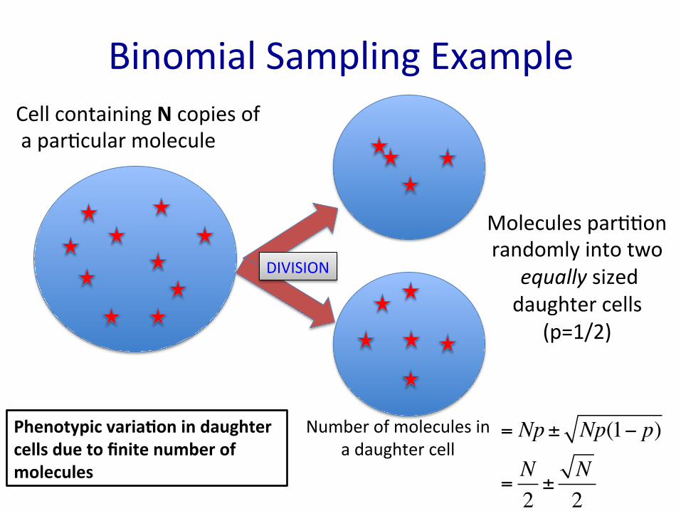
Binomial  Sampling  Example  Cell  containing  N  copies  of    a  par0cular  molecule    

Number  of  molecules  in  a  daughter  cell  

= Np± Np(1! p)

=N2±

N2

Molecules  par00on  randomly  into  two  

 equally  sized  daughter  cells  

(p=1/2)  

DIVISION  

Phenotypic  varia0on  in  daughter  cells  due  to  finite  number  of  molecules    

Rare  events:  Poisson  Distribu0on  

•  Example:  what  is  the  probability  of  observing  the  sequence  GATTACA  in  large  stretch  of  the  genome  

•  Small  probabili0es  implies  few  events  

•  Binomial  distribu0on  -­‐>  Poisson  distribu0on  in  the  rare  probability  limit    

Poisson  Distribu0on  

!

P(n;N, p) =(Np)n

n!e"Np N  >>  1  

p  <<  1  Np  fixed  

!

n = Np"2 = Np mean=variance  

coefficient  of  varia0on:     c =standard deviation

mean

=σ

�n�

=1√N

=1√Np

Poisson  Distribu0on  

•  Note  that  the  Poisson  distribu0on  only  depends  on  the  mean  <n>  

 •  Example:  the  probability  that  a  DNA  nucleo0de  is  not  sequenced  given  that  the  sequencing  coverage  is  5x  

P(n | n ) =n n

n!e! n

= P(0 | 5) = 50e!5

0!= e!5 = 0.007

Poisson  Process  •  Describes  the  distribu0on    of  random  events  •  Assump0ons:  

– The  number  of  events  in  each  interval  is  independent  of  other  events  

– The  probability  of  an  event  in  a  small  interval  is  propor0onal  to  the  interval  dura0on  

– The  probability  of  seeing  more  than  one  event  in  a  vanishing  small  interval  is  zero  

!

P(k) =(rt)k

k!e"rt

Probability  of  observing  k  events  in  0me  t:    

r  =  rate  of  events  For  a  homogeneous  process  the  rate  is  constant.  

Poisson  Process  Example:  Restric0on  sites    

Restric0on  endonuclease  EcoRI  recognizes  the  sequence  5’-­‐GAATTC-­‐3’.  The  probability  of  observing  a  par0cular  6-­‐mer  ≈  (0.25)6    ≈  2*10-­‐4  

genome            

restric0on  sites  

Model:  Homogeneous  Poisson  Process  with  rate  μ  per  base  pair  

Probability  of  n  restric0on  sites  in  segment  of  length  d       p(n) =

(µd)ne−µd

n!

Mean  number  of  restric0on  sites          

   Variance  of  restric0on  sites    

�n� = µd�(∆n)2

�≡

�(n− �n�)2

�= µd

Poisson  Process  Example:  Neural  Spike  Trains  

0   0   1   0   1   0   1   1   0   0   1   0  1   1   0  

Neural  spike    train  

Binary  representa0on.  Discre0za0on  into  small  bins  Δt  

In  small  interval  Δt,  the  probability  of  a  single  spike  =  

0me  

Δt   Tint  

Model:  Homogeneous  Poisson  Process  with  rate  r  spikes  per  unit  0me  

In  0me  interval  Tint,  the  probability  of  n  spikes  =      

volta

ge  

(rTint)ne−rTint

n!

r∆t

The  average  number  of  spikes  =    rTint

Variance  of  spike  counts  =  rTint

The Luria-Delbrück Model of evolution of Bacterial

Resistance

(Application of Poisson distribution and Fluctuation Test)

Curious experimental observation bacteria colony grows add virus (bacteriophage)

bacteria die new colony emerges

The Question

Did the mutation to resistance happen i) BECAUSE of the presence of a virus, or

ii) BEFORE adding the virus to the culture?

Two evolution models of bacterial resistance

The mutation happens…

BECAUSE of the virus (acquired immunity)

BEFORE adding the virus (mutation to immunity)

VIRUS VIRUS

Binomial ≈ Poisson distribution

Luria-Delbrück distribution

Fluctuation Test

In 1943, S.E. Luria and M. Delbrück compared the mean and variance (fluctuations) of both distributions to show that the number of mutations follows the Luria-Delbrück distribution, and not the Poisson distribution.

Mutations happen independent of the presence of viruses.

The data can then be used to estimate the mutation rate µ.

Results: variance ≠ mean

In every experiment the fluctuation of the numbers of resistant bacteria is much higher than the expectations from the hypothesis of acquired immunity.

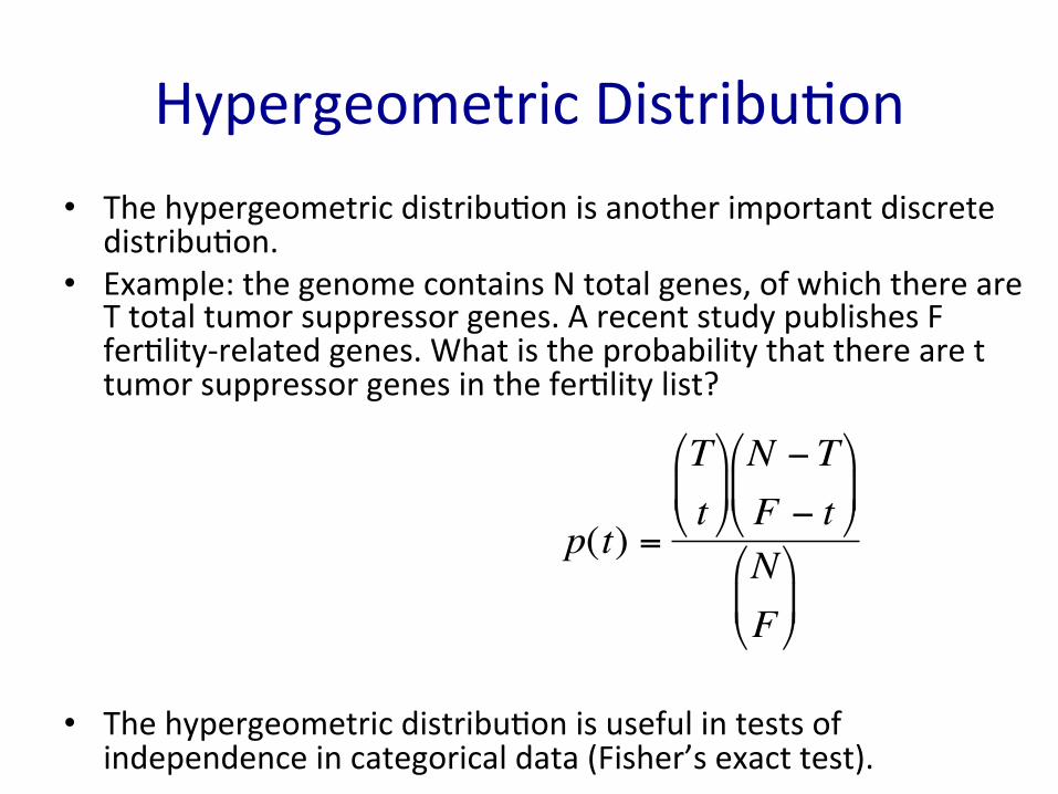
Hypergeometric  Distribu0on  •  The  hypergeometric  distribu0on  is  another  important  discrete  

distribu0on.  •  Example:  the  genome  contains  N  total  genes,  of  which  there  are  

T  total  tumor  suppressor  genes.  A  recent  study  publishes  F  fer0lity-­‐related  genes.  What  is  the  probability  that  there  are  t  tumor  suppressor  genes  in  the  fer0lity  list?    

•  The  hypergeometric  distribu0on  is  useful  in  tests  of  independence  in  categorical  data  (Fisher’s  exact  test).  

!

p(t) =

Tt"

# $ %

& ' N (TF ( t"

# $

%

& '

NF"

# $ %

& '

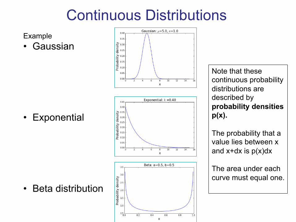
Continuous Distributions Example •  Gaussian

•  Exponential

•  Beta distribution

Note that these continuous probability distributions are described by probability densities p(x). The probability that a value lies between x and x+dx is p(x)dx The area under each curve must equal one.

Gaussian  Distribu0on  

P(x; x ,! 2 ) = 12"! 2

e!(x! x )2

2! 2

Large  N  limit  of  the  Binomial  distribu0on.      Gaussian  distribu0on  depends  only  on  mean  <x>  and  variance  σ2    Note  that  P(x;<x>,  σ2)  is  a  probability  density.    P(x;<x>,  σ2)  =  the  probability  that  a  measurement                                                                    lies  between  x  and  x+dx  

x  is  a  con0nuous    variable  

Gaussian  Distribu0on  

95%  between  μ-­‐(1.96)σ  and  μ+(1.96)σ  

Central  Limit  Theorem  

•  The  theorem  tells  us  how  the  mean/sum  of  a  set  of  independent  measurements  should  behave  

•  Let  us  take  an  arbitrary  distribu0on,  f(x),  with  mean  μ  and  standard  devia0on  σ.  We  now  take  n  samples  from  this  distribu0on  and  calculate  the  sampling  mean,  <x>=(x1+x2+…xn)/n  

•  Remarkably,  the  theorem  states  that  the  sampling  mean  <x>  will  always  follow  a  Gaussian  distribu0on  with  mean  μ  and  standard  devia0on    

!

"n

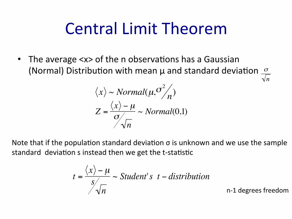
Central  Limit  Theorem  •  The  average  <x>  of  the  n  observa0ons  has  a  Gaussian  

(Normal)  Distribu0on  with  mean  μ  and  standard  devia0on    

!

x ~ Normal(µ,"2

n)!

"n

!

Z =x " µ#

n~ Normal(0,1)

Note  that  if  the  popula0on  standard  devia0on  σ  is  unknown  and  we  use  the  sample    standard    devia0on  s  instead  then  we  get  the  t-­‐sta0s0c    

!

t =x " µsn

~ Student's t " distributionn-­‐1  degrees  freedom  

Central  Limit  Theorem  

Many  Natural  Phenomena  follow  a  Gaussian  Distribu0on  

Sir  Francis  Galton  

!

P(n;N, p) =Nn"

# $ %

& ' pn (1( p)N (n

!

P(n;N, p) =12"#2

e$(n$Np )2

2# 2

!

P(n;N, p) =(Np)n

n!e"Np

BINOMIAL  

POISSON   GAUSSIAN  

(Probability  density)  

N  large  n  con0nuous  

N  large  p  small  

!

"2 = Np

! 2 = Np(1! p)n = Np

Python  code  for  distribu0ons  

Check  out  the  IPython  notebook  for  sta0s0cal  distribu0ons  and  simula0ons  of  the  central  limit  theorem:  

hsp://nbviewer.ipython.org/url/atwallab.cshl.edu/teaching/distribu0ons.ipynb  

Diffusion  Model  

0   1   2   3   4   5   6   7  -­‐1  -­‐2  -­‐3  -­‐4  -­‐5  -­‐6  -­‐7   X  

Par0cle  moves  either  lev  (L)  or  right  (R)  at  each  0me  step  Δt.  Example  sequence  of  N  steps:  LLLRLRRLRRRLLRRLRRL  

A=Total  number  of  R  steps    B=Total  number  of  L  steps  N=Total  number  of  steps=A+B  T=Total  0me=NΔt  

Displacement  at  0me  T  is  

Distribu0on  of  A  and  B  given  by  simple  Binomial  Distribu0on  

XT = A−B = A− (N −A)

= 2A−N

Diffusion  Model  Ques0on:  How  far  has  the  par0cle  been  typically  displaced  aver  0me  T?  

   i.e.,  what  are    <XT>  and  <XT2>  ?  

The  mo0on  of  a  single  par0cle  is  completely  stochas0c  and  thus  we  need  a    probabilis0c  model.  This  is  equivalent  to  observing  the  mo0on  of  a  large    collec0on  of  par0cles  with  the  same  star0ng  condi0ons.  

�XT � = 2 �A� −N�X2

T

�= 4

�A2

�− 4 �A�N +N2

To  calculate  these  quan00es  we  need  <A>  and  <A2>.  

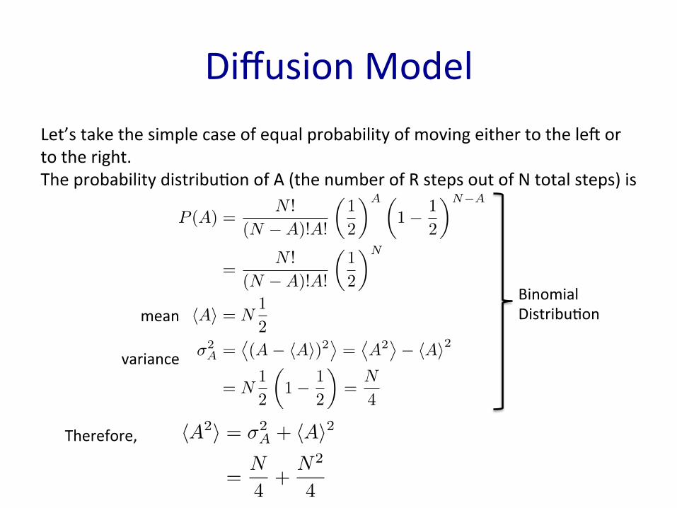
Diffusion  Model  

P (A) =N !

(N −A)!A!

�1

2

�A �1− 1

2

�N−A

=N !

(N −A)!A!

�1

2

�N

�A� = N1

2

σ2A =

�(A− �A�)2

�=

�A2

�− �A�2

= N1

2

�1− 1

2

�=

N

4

mean  

variance  

Let’s  take  the  simple  case  of  equal  probability  of  moving  either  to  the  lev  or    to  the  right.    The  probability  distribu0on  of  A  (the  number  of  R  steps  out  of  N  total  steps)  is  

Therefore,  

Binomial  Distribu0on  

�A2� = σ2A + �A�2

=N

4+

N2

4

Diffusion  Model  Plugging  the  equa0ons  for  <A>  and<A2>,  we  get  

�XT � = 2 �A� −N

= 0�X2

T

�= 4

�A2

�− 4 �A�N +N2

= N

In  terms  of  the  total  0me  T  and  the  the  diffusion  constant,  D=1/(2Δt),  we  get  �X2

T

�= 2DT

�X2

T

�1/2= (2DT )1/2

The  spread  of  a  collec0on  of  par0cles  grows  as  the  square  root  of  0me.  Therefore  a  par0cle  will  take  a  0me  100  0mes  longer  to  diffuse  a  distance  10  0mes  longer.  We  derived  this  result  in  one  dimension,  but  it  holds  in  all  dimensions  

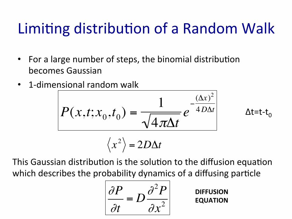
Limi0ng  distribu0on  of  a  Random  Walk  

•  For  a  large  number  of  steps,  the  binomial  distribu0on  becomes  Gaussian  

•  1-­‐dimensional  random  walk  

!

P(x, t;x0,t0) =14"#t

e$(#x )2

4D#t

!

x 2 = 2D"tThis  Gaussian  distribu0on  is  the  solu0on  to  the  diffusion  equa0on  which  describes  the  probability  dynamics  of  a  diffusing  par0cle  

!P!t

= D!2P!x2

Δt=t-­‐t0  

DIFFUSION  EQUATION  

Diffusion  Model  (large  0me)  In  the  limit  of  large  0me  T,  or  steps  N,  the  Binomial  probability  distribu0on  of  the    posi0on  of  the  diffusing  par0cle  becomes  Gaussian  with  a  0me-­‐dependent  width.  

p(X,T)   P (X,T ) =

1√4πDT

e−X2

4DT

σ =√2DT

early  T  

late  T  

width  

Gene  Regula0on  

Transcrip0on  factors  searching  for  their  specific  binding  site  using  both  three-­‐dimensional  diffusion  and  one-­‐dimensional  diffusion  along  the  DNA  molecule.    

Morphogen  gradients  DROSOPHILA  EMBRYO  

Bicoid  morphogen  freely  diffuses  along  anterior-­‐posterior  axis  

Bicoid  gradient  

Hunchback  gradient  

Bicoid  is  a  transcrip0on  factor  and  regulates  expression  of  gene  hunchback