quantitative analysis of gene expression systems - springer · quantitative analysis of gene...

Review

Quantitative analysis of gene expressionsystems

Tianshou Zhou* and Tuoqi Liu

School of Mathematics and Computational Science, Sun Yat-Sen University, Guangzhou 510275, China* Correspondence: [email protected]

Received October 23, 2015; Revised November 19, 2015; Accepted November 24, 2015

Gene expression is a complex biochemical process, involving many specific processes such as transcription,translation, switching between promoter states, and regulation. All these biochemical processes inevitably lead tofluctuations in mRNA and protein abundances. This noise has been identified as an important factor underlying theobserved phenotypic variability of genetically identical cells in homogeneous environments. Quantifying thecontributions of different sources of noise using stochastic models of gene expression is an important step towardsunderstanding fundamental cellular processes and cell-to-cell variability in expression levels. In this paper, we reviewprogresses in quantitative study of simple gene expression systems, including some results that we have not published.We analytically show how specific processes associated with gene expression affect expression levels. In particular, wederive the analytical decomposition of expression noise, which is important for understanding the roles of the factorialnoise in controlling phenotypic variability. We also introduce a new index (called attribute factor) to quantifyexpression noise, which has more advantages than the commonly-used noise indices such as noise intensity and Fanofactor.

Keywords: gene expression; chemical master equation; statistical quantities; binomial moments; expression noise

INTRODUCTION

The latest advances in biological experiments allow us tomap not only the protein-coding genes in the genomes ofprokaryotic or eukaryotic organisms but also theregulatory sequences present in these genomes. Inparticular, single-molecule and single-cell measurementsallow direct observations of real-time fluctuations in geneexpression levels in individual live cells [1–5]. A mainchallenge in the post-gene epoch is to understand how theregulatory sequences across a genome control theexpression spectrum of every gene within a cell andhow they collectively determine stochastic behavior of theentire gene regulatory network and further the cell’sfunction.Traditionally, the regulation of expression spectrum

was studied in experiments that usually measured theaverage expression level in populations consisting ofmany genetically identical cells (the number of cells usedin an experiment would be up to a few millions). Thesestudies related the average expression level of a gene to its

regulatory DNA sequence, but averaging over popula-tions often conceals differences in gene expression, whichnot only may occur between individual cells [6] but alsomay in turn have consequences for the whole multi-cellsystem or organism [7]. Therefore, this apparent draw-back of the average method makes it necessary to developother more effective methods to understand gene expres-sion in single cells as well as cell-to-cell variability inexpression spectrums.Within a single cell, gene expression is indigenously

stochastic mainly because of the following three reasons:(i) Protein-coding genes are typically present in only oneor two copies in a cell; (ii) Transcription initiation is amulti-step biochemical process; (iii) Whether a gene istranscribed at any given moment depends on the arrival ofmultiple transcription factors to their designated bindingsites. From the viewpoint of biochemical reactions, geneexpression involves transcription of DNA to mRNA,translation of mRNA to protein, transition or switchingbetween promoter activity states, feedback regulation,alternative splicing, and RNA nuclear retention [8–14].

168 © Higher Education Press and Springer-Verlag Berlin Heidelberg 2015

Quantitative Biology 2015, 3(4): 168–181DOI 10.1007/s40484-015-0056-8

All these specific biochemical processes are stochasticdue to the low copies of the involved reactive species.This stochasticity inevitably results in fluctuations inmRNA and protein abundances, and further cell-to-cellvariability in expression levels. This variability is referredto as gene expression noise, which is a main analysisobject of this paper.As a key step of gene expression, transcription takes

place often in a bursting fashion. Single-cell measure-ments have provided evidence for transcriptional burstingin prokaryotic cells [1] and in eukaryotic cells [2,15].Although the sources of transcriptional bursting remainpoorly understood [16], several lines of evidence[3,10,11,17–21] point to stochastic transitions amongthe active (ON) and inactive (OFF) states of genepromoter as an important source of expression noise,which is responsible for cell-to-cell heterogeneity inhomogeneous environments. It has been shown that incontrast to Poissonian transcription, where mRNA issynthesized in random, uncorrelated events with aprobability being uniform over time, bursty transcription,where mRNA is produced in episodes of high transcrip-tional activity (bursts) followed by long periods ofinactivity, typically leads to higher expression noise [22].Given the inherent stochasticity and complexity of gene

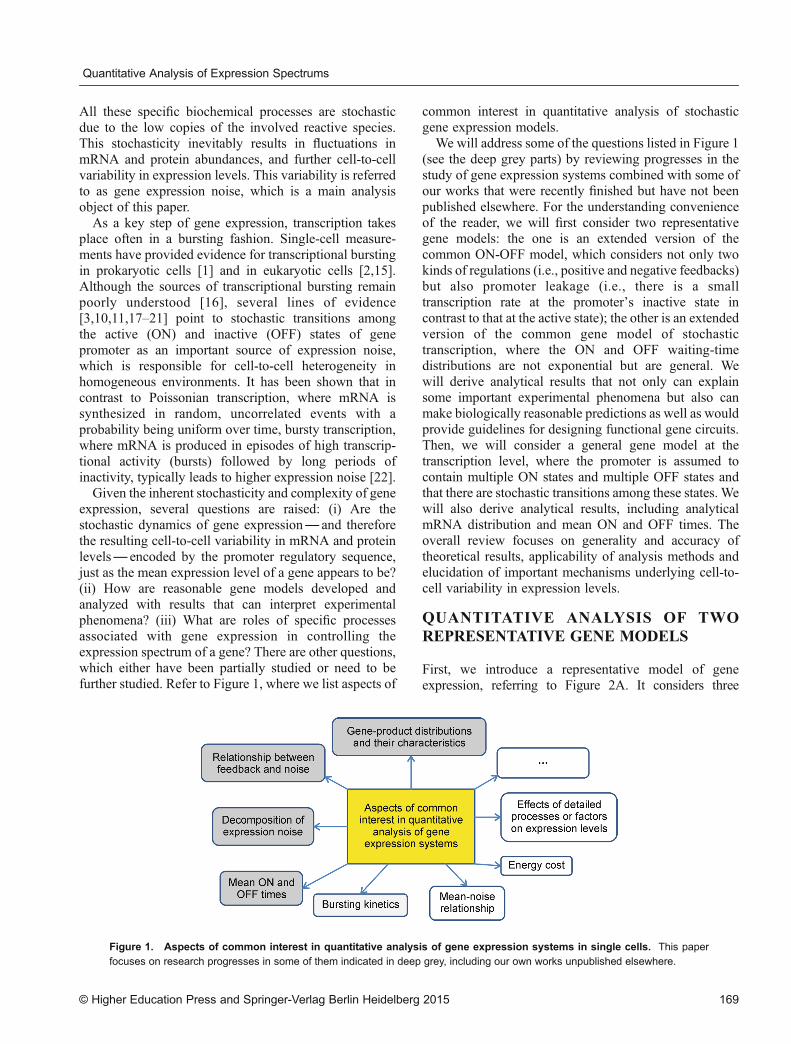
expression, several questions are raised: (i) Are thestochastic dynamics of gene expression— and thereforethe resulting cell-to-cell variability in mRNA and proteinlevels— encoded by the promoter regulatory sequence,just as the mean expression level of a gene appears to be?(ii) How are reasonable gene models developed andanalyzed with results that can interpret experimentalphenomena? (iii) What are roles of specific processesassociated with gene expression in controlling theexpression spectrum of a gene? There are other questions,which either have been partially studied or need to befurther studied. Refer to Figure 1, where we list aspects of

common interest in quantitative analysis of stochasticgene expression models.We will address some of the questions listed in Figure 1

(see the deep grey parts) by reviewing progresses in thestudy of gene expression systems combined with some ofour works that were recently finished but have not beenpublished elsewhere. For the understanding convenienceof the reader, we will first consider two representativegene models: the one is an extended version of thecommon ON-OFF model, which considers not only twokinds of regulations (i.e., positive and negative feedbacks)but also promoter leakage (i.e., there is a smalltranscription rate at the promoter’s inactive state incontrast to that at the active state); the other is an extendedversion of the common gene model of stochastictranscription, where the ON and OFF waiting-timedistributions are not exponential but are general. Wewill derive analytical results that not only can explainsome important experimental phenomena but also canmake biologically reasonable predictions as well as wouldprovide guidelines for designing functional gene circuits.Then, we will consider a general gene model at thetranscription level, where the promoter is assumed tocontain multiple ON states and multiple OFF states andthat there are stochastic transitions among these states. Wewill also derive analytical results, including analyticalmRNA distribution and mean ON and OFF times. Theoverall review focuses on generality and accuracy oftheoretical results, applicability of analysis methods andelucidation of important mechanisms underlying cell-to-cell variability in expression levels.

QUANTITATIVE ANALYSIS OF TWOREPRESENTATIVE GENE MODELS

First, we introduce a representative model of geneexpression, referring to Figure 2A. It considers three

Figure 1. Aspects of common interest in quantitative analysis of gene expression systems in single cells. This paperfocuses on research progresses in some of them indicated in deep grey, including our own works unpublished elsewhere.

© Higher Education Press and Springer-Verlag Berlin Heidelberg 2015 169

Quantitative Analysis of Expression Spectrums

kinds of fundamental biochemical processes: (i) Stochasticswitching between two promoter activity states (the activestate is denoted by A and the inactive state by I); (ii) Twokinds of regulations, i.e., positive and negative feedbacks.To derive analytical results, however, we assume thatfeedback regulation is linear although for nonlinearregulation, it is possible to derive some analytical results[23]; (iii) Promoter leakage, i.e., there is a smalltranscription rate at the OFF state, compared to that atthe ON state. Thus, our model contains most of thecommon ON-OFF models studied in the literature [24–34]as its particular case. For this model, we first derive theanalytical distribution of gene product, then give char-acteristics of statistical quantities such as noise intensityand attribute factor first introduced in this paper, and finallyanalyze the roles of factorial noise (i.e., a part of the totalnoise) in inducing the bimodal expression of gene product.Then, we introduce another representative gene model

at the transcription level, where waiting time distributionsat ON and OFF are not exponential but are general,referring to Figure 2B. For this kind of model, we firstderive an integral equation that can be used to calculatemoments of the mRNA distribution, and then give anexplicit expression for the common noise index anddiscuss its characteristics.We point that the analysis methods used to derive our

analytical results are very general, and can be applied tostochastic analysis of any reaction networks.

Explicit distribution

The distribution of the molecule numbers of the reactivespecies in a biochemical system of interest is veryimportant for understanding stochastic behavior andproperties of this system. Thus, finding this distributionis common interest although it is a challenging task inmany cases.First, we consider model (A) shown in schematic

Figure 2. The corresponding chemical master equation

(CME) reads

∂P1ðn, tÞ∂t

=– lP1ðn, tÞ þ γP0ðn, tÞ þ hnP0ðn, tÞ– gnP1ðn, tÞ þ �1[P1ðn – 1, tÞ –P1ðn, tÞ]þδ[ðnþ 1ÞP1ðnþ 1, tÞ – nP1ðn, tÞ]

∂P0ðn, tÞ∂t

=lP1ðn, tÞ – γP0ðn, tÞ – hnP0ðn, tÞþgnP1ðn, tÞ þ �0[P0ðn – 1, tÞ –P0ðn, tÞ]þδ[ðnþ 1ÞP0ðnþ 1, tÞ – nP0ðn, tÞ]

(1)

where Piðn, tÞ represents the probability that the geneproduct has n molecules at state-I (i=1 stands for ONwhereas i=0 for OFF) at time t. If the total probability isdenoted as Pðn, tÞ, then Pðn, tÞ=P0ðn, tÞ þ P1ðn, tÞaccording to the sum law of probability. In Equation (1), land γ are transition rates from ON to OFF states and viceversa, respectively; �1 and �0 are transcription rates at ONand OFF states, respectively (We assume �1 � �0 in thispaper since the latter describes promoter leakage); h and grepresent strengths of positive and negative feedbacks,respectively; and δ is the degradation rate of gene product.For convenience, we rescale all the parameters by δ in thefollowing, that is, ~l=l=δ, ~γ=γ=δ, ~h=h=δ, ~g=g=δ, and~�i=�i=δ with i=0, 1. Our interest is to find thestationary distribution PðnÞ.There are several efficient methods to find the

analytical expression of this distribution [26,31–34].Here, we adopt the Poisson representation method [35]to solve Equation 1. For this, we introduce two factorialfunctions �0ðsÞ and �1ðsÞ, which are related to twofactorial distributions P0ðnÞ and P1ðnÞ by

PiðnÞ=!smax

0�iðsÞe – s

sn

n!ds, i=0, 1 (2)

where the total function �ðsÞ=�0ðsÞ þ �1ðsÞ satisfies thenormalization condition !�ðsÞds=1 due to the prob-

ability conservative conditionX

n³0PðnÞ=1. By sub-

Figure 2. Schematic for two representative ON-OFF models of gene expression. (A) The model considers not onlyregulations but also promoter leakage; (B) The model considers ON and OFF mechanisms with general waiting-time distributions.


Tianshou Zhou and Tuoqi Liu

stituting into Equation (2), we can obtain a group ofdifferential equations regarding �0ðsÞ and �1ðsÞ. Toguarantee the uniqueness of the corresponding solution,

we impose the boundary conditions: !smax

0e – s s – ~�0ð Þ=½

1þ ~gþð Þ~h� ��ðsn=n!Þds=0, n=0, 1, 2, :::. Solving thisequation group with the given boundary conditions, weobtain the following expression of �ðsÞ

�ðsÞ=Ce~gþ~h

~gþ~hþ1sðs – ~�0Þ – 2ðα1 – sÞ

Að~gþ~hÞ~gþ~hþ1

þ1ðs – α2ÞBð~gþ~hÞ~gþ~hþ1

þ1

(3)

where C is a normalization constant. In Equation (3), wehave denoted

A=ðα1 – β1Þðα1 – β2Þ

α1 – α2, B=

ðα2 – β1Þðα2 – β2Þα2 – α1

(3A)

α1,2=1þ ~gð Þ~�0 þ 1þ ~h

� �~�1 �

ffiffiffiffiffiffiffiffiffiffiffiffiffiffiffiffiffiffiffiffiffiffiffiffiffiffiffiffiffiffiffiffiffiffiffiffiffiffiffiffiffiffiffiffiffiffiffiffiffiffiffiffiffiffiffiffiffiffiffiffiffiffiffiffiffiffiffiffiffiffiffiffiffiffiffiffiffiffiffiffiffiffiffiffiffiffiffiffiffiffi1þ ~gð Þ~�0 þ 1þ ~h

� �~�1

� �2– 4 1þ ~g þ ~h� �

~�0~�1

q2 ~g þ ~hþ 1� � (3B)

β1,2=~g~�0 þ ~h~�1 – ~l –~γ�

ffiffiffiffiffiffiffiffiffiffiffiffiffiffiffiffiffiffiffiffiffiffiffiffiffiffiffiffiffiffiffiffiffiffiffiffiffiffiffiffiffiffiffiffiffiffiffiffiffiffiffiffiffiffiffiffiffiffiffiffiffiffiffiffiffiffiffiffiffiffiffiffiffiffiffiffiffiffiffiffiffiffiffiffiffiffi~g~�0 þ ~h~�1 – ~l –~γ� �2 þ 4 ~g þ ~h

� �~l~�0 þ ~γ~�1

� �q2 ~g þ ~h� � (3C)

As such, the distribution of gene product can be formallyexpressed as

PðnÞ=C

n!!

smax

0e

– s~gþ~hþ1snðs–~�0Þ – 2ðα1–sÞ

Að~gþ~hÞ~gþ~hþ1

þ1ðs–α2ÞBð~gþ~hÞ~gþ~hþ1

þ1ds

(4)

In theory, this expression can reproduce many previously-derived distributions. Here, we give its explicit expressionsin two particular cases.In general, the promoter leakage rate, i.e., the

transcription rate at OFF state is much smaller than thatat the active state, i.e., �0 << �1. To derive the analyticalexpression of the distribution, we assume �0 � 0 forsimplicity. In this case, it is found from Equation (4) that

pðnÞ= �e�1ð Þnn!

Γðnþ αÞΓðβÞΓðαÞΓðnþ βÞ1F1 nþ α, nþ β; – �e�1ð Þ

(5)

where 1F1ða, b; zÞ=X1

n=0½ðaÞn=ðbÞn�ðzn=n!Þ with ðcÞn

being the Pochhammer symbol defined as ðcÞn=Γðcþ nÞ=ΓðcÞ is a confluent hypergeometricfunction, α=~γ= ~hþ 1

� �, β= ~lþ ~γ

� �= ~hþ ~g þ 1� �þ

~g~�1ð Þ= ~hþ ~g þ 1� �2

, a n d �= ~hþ 1� �

= ~hþ ~g þ 1� �2

.

Note that in the absence of feedback, i.e., if ~h=~g=0,the above expression can reproduce the mRNA distribu-tion in the common ON-OFF model of stochastictranscription [4,26].Then, we consider model (B) shown in Figure 2. In this

case, the mRNA distribution in general cannot beanalytically derived since waiting-time distributions aregeneral. In spite of this, we can derive integral equations

for both the moment-generating function and moments ofthe distribution. In fact, denote by W ðz; tÞ the moment-generating function of the distribution at time t, and inparticular, denote WinitðzÞ¼W ðz; 0Þ. Suppose that thereare N molecules at time t=0, where N itself is a randomvariable. Then, every mRNA at time t, which is also astochastic variable and is denoted by Xi, 1£i£N , has a

survival probability pðtÞ=1 –DðtÞ=e – δt, where DðtÞ=!

t

0δe – δsds represents the cumulative distribution function

for the mRNA lifetime. For simplicity, we assume thatthese variables Xi are independent of one another, eachfollowing a Bernoulli distribution with the moment-generating function given by MðzÞ=1þ pðtÞðez – 1Þ=1þe – δtðez – 1Þ [36–38]. Note that the total moleculenumber of mRNA at time t is given by S=X1 þ � � � þXN . Using the law of total expectation, we can know

W ðz; tÞ=Winitðlogð1þ e – δtðez – 1ÞÞÞ (6)

where we have assumed that every Xi is independent of N .In particular, at the end of an OFF-state, W ðz; toff Þ can be

given by integrating Winitðlogð1þ e – δtðez – 1ÞÞÞ over theinterval ð0, 1Þ, that is,

W ðz; toff Þ=!1

t=0Winitðlogð1þ e – δtðez – 1ÞÞÞfoff ðtÞdt (7)

where foff ðsÞ=!10Fðε, sÞdε with Fðu, sÞ representing

the joint probability density function of OFF and ONtimes is the distribution of times that the gene dwells at theOFF state (i.e., OFF times).Except that an ON-period degradation of the mRNA



molecules that have been present at the beginning of theburst continues as described above through the function1þ e – δuðez – 1Þ with Wdegðz; toff þ uÞ=Winitðlogð1þe – δðuþtoff Þðez – 1ÞÞÞ, mRNAs are also created anddegraded according to a birth-death process with anexponential waiting time. Moreover, the distribution forthis birth-death process is a Poisson distribution with the

average �u=�

δð1 – e – δuÞ and the moment-generating

function Weffectðz; toff þ uÞ=e�uðez – 1Þ [38]. Therefore,

their combination produces an effective burst size. Duringan ON-state, the probability distribution of the mRNAnumber is given by the convolution of the distribution ofthe number of those molecules that are still present fromprevious bursts and the effective burst-size distribution.This can be expressed as

W ðz; toff þ uÞ=!1

s=0Winitðlogð1þ e – δðsþuÞðez – 1ÞÞÞ

$e�uðez – 1Þfoff ðsÞds (8)

Note that one complete OFF and ON cycle defines aboundary condition:

W ðz; 0Þ=W ðz; ton þ toff Þ

=!1

s=0!

1

t=sW ðz; tÞfonðt – sÞfoff ðtÞdtds (9)

where fonðuÞ=!10Fðu, �Þd� represents the distribution

of ON times. Combining Equation (9) with Equation (6)and Equation (8), we thus arrive at the following integralequation with respect to WinitðzÞ

WinitðzÞ=W ðz; 0Þ=!1

s=0!

1

t=0Winitðlogð1þe – δðsþtÞðez–1ÞÞÞ

$e�uðez – 1ÞfonðtÞfoff ðsÞdtds (10)

which is a pivot for derivation of analytical results. Forexample, moments of the total mRNA distribution can beexpressed as

hmki= 1

τon þ τoff

$ !1

s=0hmkisð1 – f ðsÞÞdsþ!

1

u=0hmkiuð1 – gðuÞÞdu

� �(11)

with k=1, 2, where τoff=!1u=0!

1s=0

sFðu, sÞdsdu and

τon=!1s=0!

1u=0

uFðu, sÞduds are the mean OFF and ON

times respectively, whereas f ðsÞ and gðsÞ are thecumulative functions of the duration distributions at

OFF- and ON-states respectively. In Equation (11), hmkisis the kth -order moment of the mRNA distribution at timet=s during the OFF-state, which can be given by the kth -order derivative of Equation (6) at z=0, whereas hmkiu isthe kth moment of the mRNA distribution at time t=toff þu during the ON-state, which can be given by the kth -order derivative of Equation (8) at z=0.In principle, the moments obtained by Equation (11)

can be used to approximate the mRNA distribution. Infact, based on these common moments, we can calculateso-called binomial moments [39–41], which, e.g., in theone-dimensional case, are defined as

bk=Xm³k

m

k

PðmÞ=1

k!

Xm³k

mðm – 1Þ� � �ðm – kþ1ÞPðmÞ,

k=0, 1, 2, � � � (12)

where the sum function on the right-hand side can beexpressed as the linear combination of the commonoriginal moments given above. In turn, these binomialmoments can be used to reconstruct the correspondingdistribution according to the formula

PðmÞ=Xk³m

ð – 1Þm – k km

bk , m=0, 1, 2, � � � (13)

Note that unlike common moments that are divergent astheir orders go to infinity, binomial moments areconvergent as their orders go to infinity [39]. In addition,we point out that binomial moments defined above areeasily extended to cases of many random variables.

Decomposition and characteristics of expressionnoise

Noise decomposition is an interesting topic. Some authorsstudied noise decomposition in gene regulatory systems,e.g., Weinberger, et al., showed that dynamics of proteinnoise can distinguish between alternate sources ofvariability in gene expression levels [42]. Other authorsstudied noise decomposition in general biochemicalnetworks, e.g., Levchenko, et al., gave an empiricaldecomposition of the total noise (including intrinsic andextrinsic noise) in intracellular biochemical signalingnetworks using nonequivalent reporters [43], andBowsher, et al., discussed the issue of noise decomposi-tion in some biological networks and elucidated thebiological significance of their noise decomposition [44].Here, we are interested in accurate decomposition andessential characteristics of the total intrinsic noise inseveral representative models of gene expression, focus-ing on the tracing and dissecting of intrinsic noisysources.



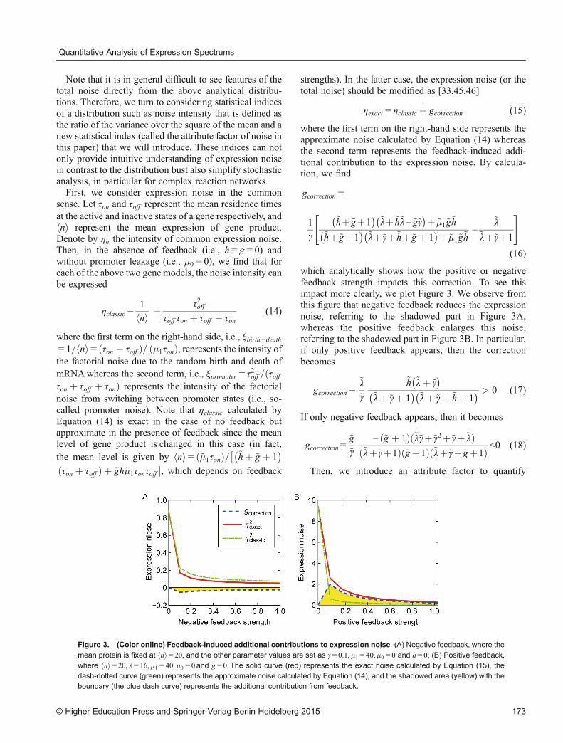
Note that it is in general difficult to see features of thetotal noise directly from the above analytical distribu-tions. Therefore, we turn to considering statistical indicesof a distribution such as noise intensity that is defined asthe ratio of the variance over the square of the mean and anew statistical index (called the attribute factor of noise inthis paper) that we will introduce. These indices can notonly provide intuitive understanding of expression noisein contrast to the distribution bust also simplify stochasticanalysis, in particular for complex reaction networks.First, we consider expression noise in the common

sense. Let τon and τoff represent the mean residence timesat the active and inactive states of a gene respectively, andhni represent the mean expression of gene product.Denote by ηn the intensity of common expression noise.Then, in the absence of feedback (i.e., h=g=0) andwithout promoter leakage (i.e., �0=0), we find that foreach of the above two gene models, the noise intensity canbe expressed

ηclassic=1

hni þ τ2offτoff τon þ τoff þ τon

(14)

where the first term on the right-hand side, i.e., �birth – death=1=hni=ðτon þ τoff Þ= ð�1τonÞ, represents the intensity ofthe factorial noise due to the random birth and death ofmRNAwhereas the second term, i.e., �promoter=τ2off =ðτoffτon þ τoff þ τonÞ represents the intensity of the factorialnoise from switching between promoter states (i.e., so-called promoter noise). Note that ηclassic calculated byEquation (14) is exact in the case of no feedback butapproximate in the presence of feedback since the meanlevel of gene product is changed in this case (in fact,the mean level is given by hni= ~�1τonð Þ= ~hþ ~g þ 1

� ��ðτon þ τoff Þ þ ~g~h~�1τonτoff �, which depends on feedback

strengths). In the latter case, the expression noise (or thetotal noise) should be modified as [33,45,46]

ηexact=ηclassic þ gcorrection (15)

where the first term on the right-hand side represents theapproximate noise calculated by Equation (14) whereasthe second term represents the feedback-induced addi-tional contribution to the expression noise. By calcula-tion, we find

gcorrection=

1

~γ

~hþ~gþ1� �

~lþ~h~l – ~g~γ� �þ ~�1~g~h

~hþ~gþ1� �

~lþ~γþ~hþ~g þ 1� �þ ~�1~g~h

–~l

~lþ~γþ1

" #(16)

which analytically shows how the positive or negativefeedback strength impacts this correction. To see thisimpact more clearly, we plot Figure 3. We observe fromthis figure that negative feedback reduces the expressionnoise, referring to the shadowed part in Figure 3A,whereas the positive feedback enlarges this noise,referring to the shadowed part in Figure 3B. In particular,if only positive feedback appears, then the correctionbecomes

gcorrection=~l

~γ

~h ~lþ ~γ� �

~lþ ~γþ 1� �

~lþ ~γþ ~hþ 1� � > 0 (17)

If only negative feedback appears, then it becomes

gcorrection=~g

~γ– ð~g þ 1Þð~l~γþ~γ2þ~γþ~lÞ

ð~lþ~γþ1Þð~gþ1Þð~lþ~γþ~gþ1Þ <0 (18)

Then, we introduce an attribute factor to quantify

Figure 3. (Color online) Feedback-induced additional contributions to expression noise (A) Negative feedback, where the

mean protein is fixed at hni=20, and the other parameter values are set as γ=0:1,�1=40,�0=0 and h=0; (B) Positive feedback,where hni=20, l=16,�1=40,�0=0and g=0:The solid curve (red) represents the exact noise calculated by Equation (15), thedash-dotted curve (green) represents the approximate noise calculated by Equation (14), and the shadowed area (yellow) with the

boundary (the blue dash curve) represents the additional contribution from feedback.



expression noise. Analogous to the definition of commonnoise intensity, we define the attribute factor as the ratio ofthe double of the second-order binomial moment over thesquare of the first-order binomial moment

�attribute=2b2b21

(19)

One will see that this factor has more advantages than thenoise intensity in quantifying characteristics of expressionnoise.In order to help understand this factor, let us

consider the simplest birth-death process described by

Æ ↕ ↓

gX ↕ ↓

δÆ. For this reaction model, we know that the

molecule number of X follows a Poisson distribution,PðnÞ=e – lln=n!, where l=g=δ is a characteristic para-meter of this distribution. Recall that the size of the Fanofactor defined as the ratio of variance over mean can beused to judge whether a distribution is Poissonian [47].Specifically, the distribution is sub-Poissonian if the Fanofactor is less than 1; it is Poissonian if the Fano factor isequal to 1; and it is sup-Poissonian if the Fano factor ismore than 1. Similarly, for the attribute factor introducedabove, we have that if �attribute<1, then the distribution issub-Poissonian; if �attribute=1, then the distribution isPoissonian; and if �attribute > 1, then the distribution issup-Poissonian.Interestingly, we find that for the common ON-OFF

gene model at the transcription level, the attribute factor�attribute is given by

�attribute=~�birth – death þ �promoter

=1þ τ2offτon þ τoff þ τonτoff

> 1 (20)

which depends only on promoter structure but is irrelativeto the transcription rate. Thus, the mRNA distribution issup-Poissonian for this gene model. In the presence offeedback but without promoter leakage, we can show

�attribute=1þ 1

~γ

~lþ ~h~l – ~g~γþ ~�1~g ~hþ 1� �

~hþ ~g þ 1

~lþ ~γþ ~hþ ~g þ 1þ ~�1~g~hþ ~g þ 1

þ~lþ ~γ� �

~hþ ~g þ 1� �þ ~g~�1

~γ~�1> 1 (21)

This indicates that the mRNA distribution is also sup-Poissonian.We point out the following three points: (i) the above

analysis gives partial reasons why �attribute is called theattribute factor; (ii) the attribute factor has many other

advantages, e.g., it contains useful information onbursting kinetics; (iii) the above analytical results providequantitative descriptions of essential intracellular pro-cesses. The related results for the first and second pointswill be published elsewhere.

Roles of factorial noise in controlling phenotypicvariability

In this subsection, we investigate the role of factorialnoise in controlling cellular phenotype (e.g., bimodality).From the above subsection, we know that the expressionnoise is composed of two parts: the one is from the birthand death of gene product and the other from stochasticswitching between promoter states. Each part is called asfactorial noise in this paper. As is well known, thedistribution of gene product in an ON-OFF model canexhibit one peak or two distinct peaks, which correspondto different cellular phenotypes. Thus, a natural questionis what the role of factorial noise is in inducingunimodality or bimodality.For simplicity, we consider the common ON-OFF

model at the transcription level, implying that we considerneither regulation nor promoter leakage. In this case, weadopt two approximations to elucidate the roles of twonoisy sources in inducing bimodality [31]: continuousapproximation and adiabatic approximation.First, we consider continuous approximation. If the

characteristic number of gene products (i.e., proteins) isvery large as that in the deterministic case (i.e.,M=�1=δ � 1), then the ratio (or concentration) x=n=M may be considered as a continuous variable. Thus, wecan easily derive the corresponding CME. By solving thisequation, we obtain

PðxÞ=Ce hþgð Þxð1 – xÞ~γþg – 1 x – ~�0=~�1ð Þh~�0þ~l~�1

~�1– 1

(22)

where h=~h~�1, g=~g~�1, and C is a normalization constant

determined by !1

0PðxÞ=1.

Then, we consider adiabatic approximation. If theprotein number fluctuations become significant comparedto those from switching between promoter activity states(e.g., in prokaryotic cells), the CME will be reduced toanother simpler model, where all the gene states aresimply integrated by fast equilibrium. In this simplifiedmodel, the dominant noise is transcriptional or transla-tional noise, which is generated due to the stochastic birthand death of protein. Moreover, the protein distribution isgiven by

PðnÞ= 1

1F1 α, β; e�1ð Þe�1ð Þnn!

ðαÞnðβÞn

(23)

where α= ~γ~�1 þ ~l~�0

� �= ~h~�1

� �and β=~�1.



In order to characterize the above two approximations,we introduce a ratio, which is defined as

Ratio=promoter noise

synthesis noise(24)

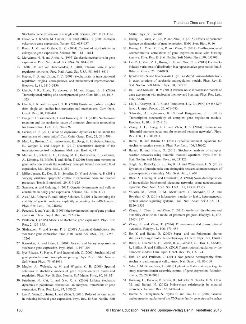
Apparently, promoter noise is dominant if Ratio � 1whereas translational noise is dominant if Ratio << 1.Thus, the former corresponds to the continuous approx-imation whereas the latter to the adiabatic approximation.Figure 4 shows how factorial noise can induce bimodality.It should be pointed out that the above analysis can also

obtain the decomposition of expression noise (Actually,we only can the formal expression according to the noisedefinition). Compared to the derived-above analyticaldecomposition in which the noisy sources are practicallyartificial, the former decomosition is essential since thetraced sources of noise are releastic. However, thedifference between them is not too big under someassumed conditions (detailed discussions are omittedhere).

QUANTITATIVE ANALYSIS OF AGENERAL GENE MODEL

Complex promoters with more than two states are not theexception but the rule as combinatorial control of generegulation by multiple species of transcription factors, andthe latter case is widespread in eukaryotic cells [48]. Eventhose promoters that are regulated by a single transcrip-tion factor may have multiple states [2,49]. For bacterialcells, the promoters that are often viewed as simple canexist in a surprisingly large number of regulatory states.For example, the PRM promoter of phage lambda in E.coli is regulated by two different transcription factors

binding to two sets of three operators that can be broughttogether by looping out the intervening DNA. As a result,the number of regulatory states of the PRM promoter is upto 128 [50]. In contrast, eukaryotic promoters are morecomplex, involving nucleosomes competing with or beingremoved by transcription factors [51]. In addition to theconventional regulation by transcription factors, theeukaryotic promoters can be also epigenetically regulatedvia histone modifications [52–54]. Such regulation maylead to very complex promoter kinetics [52].Based on the above reasons, we introduce a general

gene model at the transcription level, where the genepromoter contains many activity states due to differentbindings of transcription factors to regulatory sites onDNA or other unspecified mechanisms. These activitystates (N in total) are divided as L active states and K(=N – L) inactive states. For analysis convenience, we donot consider regulation. We use matrix A=ðaijÞ todescribe promoter activity, diagonal matrix Λ=diagð�1,�2, � � � , �N Þ to describe exits of transcription from DNAto mRNA, and diagonal matrix δ=diagðδ1, δ2, � � � , δN Þto describe degradation of mRNA at promoter activitystates. Let PkðmÞ represent the distribution that mRNAhas m molecules at state-k of the promoter and P=ðP1, � � � , PN ÞT represent the column vector consisting ofthese factorial probabilities. Then, the CME for thecorresponding gene model can be expressed as

dPðm; tÞdt

=APðm; tÞ þ δðE – IÞ[mPðm; tÞ]

þΛðE – 1 – IÞ[Pðm; tÞ] (25)

where E is a vector of step operators and I is a vector ofunit operators. Interestingly, the time-evolution equations

Figure 4. (Color online) Phase diagrams describing how stochastic bimodality is generated (A) Slow switching, where

l=γ=0:5; (B) Fast switching, where l=20 and γ=2: In (A) and (B), the gray curve represents the monstable state in thedeterministic case, and blue, dashed green and dot-dashed red curves each representing the noise-induced stable state in thestochastic case correspond respectively to the high state where the protein number is large, the middle state where the protein

number is moderate (corresponding to the valley between two peaks of the distribution) and the low state where the protein numberis small.



for the binomial moments defined above take thefollowing simpler form in contrast to the CME

d

dtbk=Abk þ Λbk – 1 – kδbk (26)

where k=1, 2, � � �. Clearly, the first term on the right-hand side of Equation (26) describes kinetics of thepromoter with the transition matrix A that is actually anM-matrix (since the sum of every column elements isequal to zero), the second term describes the exits oftranscription with the transcription matrix Λ, and the thirdterm describes the degradation dynamics of mRNA withthe degradation matrix δ (throughout this paper, weconsider only the same degradation rate for simplicity,and denote it as δ). We point out that model (26) includesall previously-studied models of mRNA expression as itsparticular cases.

mRNA distributions

For simplicity, we consider a particular case, i.e., assumeall the degradation rates are equal: δ1=δ2= � � �=δN=δ(implying that the degradation matrix takes the form ofδ=δIN with IN being the unit matrix). In addition, werescale all the parameters by δ for convenience. In thefollowing, we are only interested in the steady-statemRNA distribution.Note that when solving Equation (26), we need to know

the expression of b0=ðbð1Þ0 , bð2Þ0 , � � � , bðNÞ0 ÞT , which can

be given by noting the fact that the transition matrix A isan M-matrix (i.e., the sum of every column elements isequal to zero). By solving uNb0=1 and Ab0=0, whereuN=ð1, 1, � � � , 1Þ is an N – dimensional row vector, wefind

bðkÞ0 =∏N – 1

i=1

βðkÞi

αi, 1£k£N (27)

where 0, – α1, – α2, � � � , – αN – 1 are the characteristic

values of the rescaled matrix ~A and – βðkÞ1 , – βðkÞ2 , � � � ,– βðkÞN – 1 are the eigenvalues of the matrix Mk that is theminor one of the N � N matrix ~A by crossing out the kth

row and kth column of its entry ~akk .

Also note that the total distribution is given by PðmÞ=XN

k=1Pk and the order-k binomial moment is

calculated according to bk=XN

i=1bðiÞk =uN⋅bk . Thus,

it follows from Equation (26) that

bn=1

n!∏nk=1det kI – ~A

� � uN∏1

k=nkI – ~A� �� ~Λ� �

b0 ,

n=1, 2, � � � (28)

where kI – ~A� ��

and det kI – ~A� �

are the adjacency matrix

and the determinant of matrix kI – ~A� �

, respectively.Once all the binomial moments are given by Equation(28), we can calculate the mRNA distribution accordingto the above Equation (13).Now, we consider distributions in several particular

cases. If all the rescaled transcription rates are equal, i.e.,~�1=~�2= � � �=~�N=~� (implying that the rescaled tran-scription matrix takes the form of ~Λ=~�IN ), then thenumber of mRNA molecules always follows a Poissoniandistribution, independent of promoter structure. This is aninteresting fact. If transcription matrix takes the form of~Λ=~� 0ðN – 1Þ 0

0 1

, then the mRNA distribution takes

the form

PðmÞ= e�m

m!∏N – 1

i=1

ðβðNÞi ÞmðαiÞm

$N – 1 FN – 1mþ β Nð Þ

1 , � � � , mþ β Nð ÞN – 1

mþ α1, � � � , mþ αN – 1

��; – e�� ,

m=0, 1, 2, � � � (29)

where nFna1, � � � , anb1, � � � , bn

j;��

is a confluent hypergeo-

metric function [55]. If the rescaled transcription matrix

takes the form: ~Λ=~� IðN – 1Þ 00 0

, then the mRNA

distribution

PðmÞ= e –e�m!

Xmk=0

m

k

e�m – kð – 1Þk

$ ∏N – 1

i=1

ðβðNÞ1 ÞkðαiÞk N – 1FN – 1

k þ βðNÞ1 , � � � , k þ βðNÞ

N – 1

k þ α1, � � � , k þ αN – 1

��; e�� (30)

In particular, for the common ON-OFF model ofstochastic transcription, we find that the resultingmRNA distribution obtained by Equation (13) combinedwith Equation (28) can reproduce the one obtained inprevious studies [4]. That is,

pðmÞ= e�m

m!

Γ elþ m

Γ elþeγ Γ elþeγþ m

Γ el $1F1

elþ m, elþeγþ m; – e� (31)

Waiting time distributions and mean waiting times

As is seen from the above, the mean ON and OFF times



are important for calculating the mean mRNA level andstudying the mRNA noise. In the case that the genepromoter has multiple ON and OFF states, in order to givemean ON and OFF times, we need to calculate thedistributions of ON and OFF times.Let matrices A11 and A00 describe transitions among

the active states and among the inactive states, respec-tively. The matrix A10 describes how the active statestransition to the inactive states. Similarly, we canintroduce matrix A01. Denote by A=ðaijÞ the N � Ntransition matrix, which consist of four block matricesA11, A00, A10 and A01. Matrix Λ=diagð�1, � � � , �N Þdescribes exits of transcription with �i representing thetranscription rate of mRNA in state-i (�i=0 means that notranscription takes place). Thus, two matrices A and Λaltogether determine the promoter structure completelyAssume that the promoter states begin to transition

from OFF (ON) to ON (OFF) at time t=0. Define

Qð1Þi ðτÞ ði=1, � � � , LÞ and Qð0Þ

k ðτÞ ðk=1, � � � , KÞas the subsequent “survival” probabilities that thepromoter is still at the ith ON and at the kth OFF state at

time t=τ > 0, respectively. If we denote Qð0ÞðτÞ=ðQð0Þ

1 ðτÞ, � � � , Qð0ÞK ðτÞÞT and Qð1ÞðτÞ=ðQð1Þ

1 ðτÞ, � � � ,Qð1Þ

L ðτÞÞT, then according to the corresponding CME,we can show

Qð0ÞðτÞ=expðA00τÞQð0Þð0Þ

Qð1ÞðτÞ=expðA11τÞQð1Þð0Þ(32)

Thus, for two given sets of initial survival probabilities

fQð0Þ1 ð0Þ, � � � , Qð0Þ

K ð0Þg and fQð1Þ1 ð0Þ, � � � , Qð1Þ

L ð0Þg,the distribution functions for the dwell times τ at theOFF and ON states are given by

~f off ðτÞ=uLA01Qð0ÞðτÞ=uLA01expðA00τÞQð0Þð0Þ

~f onðτÞ=uKA10Qð1ÞðτÞ=uKA10expðA11τÞQð1Þð0Þ

(33)

From Equation (33), we can see that each of twodistribution functions is in general a linear combinationof exponential functions of the form eljτ , so the result hereis an extension of that in [56–58]. Furthermore, the OFFand ON times can be computed by substituting ~f off ðτÞ,~f onðτÞ into the general expression ~τ=!

10τf ðτÞdτ, that is,

~τoff=!1

0τuLA01expðA00τÞQð0Þð0Þdτ

=uLA01ðA00Þ – 2Qð0Þð0Þ

~τon=!1

0τuKA10expðA11τÞQð1Þð0Þdτ

=uKA10ðA11Þ – 2Qð1Þð0Þ (34)

Note that Equation (34) is not the resulting meanwaiting times at OFF and ON states since the initialsurvival probabilities Qð0ÞðτÞ and Qð1ÞðτÞ depend on thetransition pattern among ON and OFF states. For a givenpromoter structure, to obtain the total OFF and ON dwelltimes, we require to average h~τoff i or h~τoni over all suchON states that transition to OFF states or over all suchOFF states that transition to ON states. For example, to

compute the resulting fonðτÞ, one should choose Qð1jÞi ð0Þ

¼ðXL

l=1að0↕ ↓1Þil =

XK

k=1

XL

l=1að0↕ ↓1Þkl Þδij ðj, i=1, � � � ,

KÞ as the initial conditions, where δij is the Kronecker

delta, and for clarity, we let að0↕ ↓1Þik represent the transition

rate from the kth OFF state to the ith ON state (similarly,

að1↕ ↓0Þik , að0↕ ↓0Þ

ik and að1↕ ↓1Þik ). The resulting distribution

functions for the mean ON and OFF times are given by

foff ðτÞ=uLA01expðA00τÞA10uTL

fonðτÞ=uKA10expðA11τÞA01uTK

(35)

Correspondingly, the resulting mean dwell times at OFFand ON states are given by

τoff=1

uLA10uTL

uLA01ðA00Þ – 2A10uTL

τon=1

uKA01uTK

uKA10ðA11Þ – 2A01uTK

(36)

One can use the common ON-OFF model to verify thecorrectness of the above analytical expressions.

Decomposition and characteristics of the mRNAnoise

First, note that the common noise (i.e., it is defined as theratio of variance over the square of mean) in a reactivespecies of interest in any reaction network can becalculated using the first two binomial moments. Thatis, we have the following general formula

η=1

b1þ 2b2 – b

21

b21(37)

Second, for the above gene model with generalpromoter structure, we find that the mRNA noise isgiven by



ηm=1

hmi þ∏N – 1

i=1

βðNÞi

αi∏N – 1

i=1

1þ βðNÞi

1þ αi– ∏N – 1

i=1

βðNÞi

αi

" #

∏N – 1

i=1

βðNÞi

αi

!2 (38)

where hmi= ~�τonð Þ=ðτoff þ τonÞ. Like the case of thecommon ON-OFF model, the first term on the right-handside of Equation (38) represents the birth-death noise ofmRNA whereas the second term represents the promoternoise. In other words, we have the following decomposi-tion formula for the mRNA noise in any case

ηm=�birth – death þ �promoter (38)

\ Third, we give the decomposition of the mRNA noiseusing the attribute factor introduced above. It is easy toverify that the attribute factor can be expressed as

�attribute=1þ∏N – 1

i=1

βðNÞi

αi∏N – 1

i=1

1þ βðNÞi

1þ αi– ∏N – 1

i=1

βðNÞi

αi

" #

∏N – 1

i=1

βðNÞi

αi

!2 (39)

which is independent of the transcription rate �. Recallthat ð2b2Þ=b21 represents the burst size [59]. Thus, for theabove general model of stochastic transcription, theattribute factor can describe not only the level of theexpression noise but also the burst size.In addition, if the gene promoter has one active state

and L inactive states, which altogether form a loop withunidirectional transcription between every two neighbor-ing states, then the mRNA noise intensity can beexpressed as

ηm=1

hmi þ ðτon þ τoff Þ∏Lk=1ð1þ τkÞ

ð1þ τonÞ∏Lk=1ð1þ τkÞ – 1

– 1 (40)

Finally, we show how the number of the inactive statesimpacts the noise intensity in the common sense. If the

total OFF time is fixed, i.e.,XN – 1

k=1τk=cosntant, then

we have

ηm³ηmin=1

hmi þ ðτon þ τoff Þðτoff =Lþ 1ÞLð1þ τonÞðτoff =Lþ 1ÞL – 1 – 1 (41)

Note that the function f ðLÞ=ðτoff =Lþ 1ÞL=[ð1þ τonÞðτoff =Lþ 1ÞL – 1] is monotonically decreasing with theincrease of L, so the noise intensity (ηm) achieves themaximum at L=1 that corresponds to the common two-state gene model (we denote by ηon – off the correspondingnoise intensity). Therefore,

ηm<ηon – off (42)

unless L=1. Since the actual OFF mechanism corre-sponds to L > 1 [10], we obtain an important biologicalconclusion, i.e., the multi-OFF mechanism alwaysreduces the noise in contrast to the common ON-OFFmechanism. This implies that the common ON-OFFmodel overestimates the noise in gene expression in thereal case.

SUMMARY AND DISCUSSION

Gene expression is one of the important research contentsof systems biology since it is the core of intracellularprocesses. While recent advances in experimental meth-ods allow direct observations of real-time fluctuations ingene expression levels in individual live cells [1–5], thereis considerable interest in theoretically understandinghow different molecular mechanisms of gene expressionimpact variations in mRNA and protein levels across apopulation of cells. By analyzing two representative genemodels (Figure 2) and a general gene model at thetranscription level, we have shown that the moleculenumber of gene product in general follows a distributionexpressed by a confluent hypergeometric function. Wehave also shown that in the absence of feedback,expression noise can be decomposed into the simplesum of the birth-death noise and transcription noise. In thepresence of feedback, however, we have found that thefeedback can induce additional contribution to expressionnoise. In particular, the multi-OFF mechanism alwaysplays a role of reducing expression noise in contrast to thecommon ON-OFF mechanism. These results are inde-pendent of choice of system parameters and are thereforequalitative.As is pointed out in the introduction, gene expression

involves other biochemical processes such as alternativesplicing [50,61] and RNA nuclear retention [62], apartfrom transcription, translation and feedback regulation. Infact, gene expression processes are becoming clearer dueto the occurrence of new experimental technologies. Onecan imagine that these detailed processes would impactexpression levels in their own ways. For quantitativeanalysis of this impact, one may take some methods andindices used in this paper, such as binomial momentmethod and attribute factor. In addition, we point out thatthis paper has focused on analysis of intrinsic noise, butextrinsic noise can also exist in gene expression systems.Analyzing contributions of extrinsic noise to cell-to-cellvariability and dissecting decomposition principles of thetotal noise as done in this paper are challenging taskssince source of extrinsic noise may be complex.In this paper, we have reviewed some progresses in the

study of several gene expression systems, focusing onmodeling and analysis as well as elucidation of the related



mechanisms. Even for these systems, however, there aresome other questions that are also interesting butunsolved. Here, we list only partial and unsolvedquestions, and give frameworks for their quantitativeanalysis.

Differences between transient and stationarydynamics of gene expression

Many dynamical systems may exhibit very differentsteady-state and transient dynamics. In particular, thereare big differences between stationary and transientbehaviors of gene expression systems, mainly becauseof stochastic switching between promoter activity states.For example, for the common ON-OFF model of geneexpression, the time-evolutional distribution may exhibitbimodalities of different modes although the correspond-ing steady-state distribution is unimodal [46]. For steady-state dynamics, this paper has given nice, analyticaldescriptions. For transient dynamics, however, it seemsimpossible to give analytical descriptions. In spite of this,numerical simulation based on the Gillespie stochasticalgorithm [63] or on the binomial moment methodmentioned in this paper may give quantitative descrip-tions for differences between two distinct behaviors.

Inferring promoter structure based on expressionspectrums

While expression spectrums observed in experiments arecomprehensive consequences of gene expression, thenumber of promoter activity states in eukaryotic organ-isms may be up to 128 [50]. A question naturally arises:how is promoter structure inferred from experimentaldata? This question is interesting but challenging. Apossible way of solving the question is to analyze andcompare all the possible modes of steady-state andtransient distributions and find differences between them.For example, for the common ON-OFF model at thetranscription level, all the possible modes of the mRNAdistribution are only those: two modes of unimodality,where the peak is close to the origin and the peak is awayfrom the origin; one mode of bimodality, where one peakis close to the origin whereas the other peak is away fromthe origin [46]. If the promoter has activity states of morethan one, then the modes of the mRNA distribution maybe complex but different from those in the case of onlytwo activity states.

The mean-noise relationship

Mathematically, the mean-noise relationship is formu-lated as

logð�2=�2Þ=βlog�þ logα (43)

where �2 and � represent the variance and the mean ofmRNA or protein, respectively. In Equation (43), both αand β are two constants depending on the parameters of astochastic system of interest. For this formulation, the keyis to determine the sign and size of β since β represents theslope of the line in the ðlog�, logð�2=�2ÞÞ plane. Forsystems of gene expression, there are many works tostudy the relationship between mean and noise [64–66],some of which showed that β is negative [64] whereasothers showed it may be positive or negative [65]. Anunsolved question is what mechanisms govern the mean-noise relationship, in particular the sign and size of β.Owing to potential applications of this relationship in,e.g., disease systems [66], this question deserves study.Note that �2=�2 represents the noise intensity. Therefore,one may use the results given in this paper to analyze themean-noise relationship in some cases.

ACKNOWLEDGEMENTS

This work was partially supported by Grant Nos. 91230204 (T. Z.),

91530320 (T. Z.), 2014CB964703 and 20120171110047 (T. Z.).

COMPLIANCE WITH ETHICS GUIDELINES

The authors Tianshou Zhou and Tuoqi Liu declare that they have no conflict

of interests.

This article does not contain any studies with human or animal subjects

performed by any of the authors.

REFERENCES

1. Golding, I., Paulsson, J., Zawilski, S. M. and Cox, E. C. (2005) Real-

time kinetics of gene activity in individual bacteria. Cell, 123, 1025–

1036

2. Raj, A., Peskin, C. S., Tranchina, D., Vargas, D. Y. and Tyagi, S. (2006)

Stochastic mRNA synthesis in mammalian cells. PLoS Biol., 4, e309

3. Suter, D. M., Molina, N., Gatfield, D., Schneider, K., Schibler, U. and

Naef, F. (2011) Mammalian genes are transcribed with widely different

bursting kinetics. Science, 332, 472–474

4. Harper, C. V., Finkenstädt, B., Woodcock, D. J., Friedrichsen, S.,

Semprini, S., Ashall, L., Spiller, D. G., Mullins, J. J., Rand, D. A.,

Davis, J. R., et al. (2011) Dynamic analysis of stochastic transcription

cycles. PLoS Biol., 9, e1000607

5. Spiller, D. G., Wood, C. D., Rand, D. A. and White, M. R. H. (2010)

Measurement of single-cell dynamics. Nature, 465, 736–745

6. Raj, A. and van Oudenaarden, A. (2008) Nature, nurture, or chance:

stochastic gene expression and its consequences. Cell, 135, 216–226

7. Blake, W. J., Balázsi, G., Kohanski, M. A., Isaacs, F. J., Murphy, K. F.,

Kuang, Y., Cantor, C. R., Walt, D. R. and Collins, J. J. (2006)

Phenotypic consequences of promoter-mediated transcriptional noise.

Mol. Cell, 24, 853–865

8. Ozbudak, E. M., Thattai, M., Kurtser, I., Grossman, A. D. and van

Oudenaarden, A. (2002) Regulation of noise in the expression of a

single gene. Nat. Genet., 31, 69–73

9. Elowitz, M. B., Levine, A. J., Siggia, E. D. and Swain, P. S. (2002)



Stochastic gene expression in a single cell. Science, 297, 1183–1186

10. Blake, W. J., KAErn, M., Cantor, C. R. and Collins, J. J. (2003) Noise in

eukaryotic gene expression. Nature, 422, 633–637

11. Raser, J. M. and O’Shea, E. K. (2004) Control of stochasticity in

eukaryotic gene expression. Science, 304, 1811–1814

12. McAdams, H. H. and Arkin, A. (1997) Stochastic mechanisms in gene

expression. Proc. Natl. Acad. Sci. USA, 94, 814–819

13. Thattai, M. and van Oudenaarden, A. (2001) Intrinsic noise in gene

regulatory networks. Proc. Natl. Acad. Sci. USA, 98, 8614–8619

14. Kepler, T. B. and Elston, T. C. (2001) Stochasticity in transcriptional

regulation: origins, consequences, and mathematical representations.

Biophys. J., 81, 3116–3136

15. Chubb, J. R., Trcek, T., Shenoy, S. M. and Singer, R. H. (2006)

Transcriptional pulsing of a developmental gene. Curr. Biol., 16, 1018–

1025

16. Chubb, J. R. and Liverpool, T. B. (2010) Bursts and pulses: insights

from single cell studies into transcriptional mechanisms. Curr. Opin.

Genet. Dev., 20, 478–484

17. Boeger, H., Griesenbeck, J. and Kornberg, R. D. (2008) Nucleosome

retention and the stochastic nature of promoter chromatin remodeling

for transcription. Cell, 133, 716–726

18. Larson, D. R. (2011) What do expression dynamics tell us about the

mechanism of transcription? Curr. Opin. Genet. Dev., 21, 591–599

19. Mao, C., Brown, C. R., Falkovskaia, E., Dong, S., Hrabeta-Robinson,

E., Wenger, L. and Boeger, H. (2010) Quantitative analysis of the

transcription control mechanism. Mol. Syst. Biol., 6, 431

20. Mariani, L., Schulz, E. G., Lexberg, M. H., Helmstetter, C., Radbruch,

A., Löhning, M., Höfer, T. and Höfer, T. (2010) Short-term memory in

gene induction reveals the regulatory principle behind stochastic IL-4

expression. Mol. Syst. Biol., 6, 359

21. Miller-Jensen, K., Dey, S. S., Schaffer, D. V. and Arkin, A. P. (2011)

Varying virulence: epigenetic control of expression noise and disease

processes. Trends Biotechnol., 29, 517–525

22. Sanchez, A. and Golding, I. (2013) Genetic determinants and cellular

constraints in noisy gene expression. Science, 342, 1188–1193

23. Assaf, M., Roberts, E. and Luthey-Schulten, Z. (2011) Determining the

stability of genetic switches: explicitly accounting for mRNA noise.

Phys. Rev. Lett., 106, 248102

24. Peccoud, J. and Ycart, B. (1995) Markovian modelling of gene product

synthesis. Theor. Popul. Biol., 48, 222–234.

25. Paulsson, J. (2005) Models of stochastic gene expression. Phys. Life

Rev., 2, 157–175.

26. Shahrezaei, V. and Swain, P. S. (2008) Analytical distributions for

stochastic gene expression. Proc. Natl. Acad. Sci. USA, 105, 17256–

17261

27. Karmakar, R. and Bose, I. (2004) Graded and binary responses in

stochastic gene expression. Phys. Biol., 1, 197–204

28. Iyer-Biswas, S., Hayot, F. and Jayaprakash, C. (2009) Stochasticity of

gene products from transcriptional pulsing. Phys. Rev. E: Stat. Nonlin.

Soft Matter Phys., 79, 031911

29. Mugler, A., Walczak, A. M. and Wiggins, C. H. (2009) Spectral

solutions to stochastic models of gene expression with bursts and

regulation. Phys. Rev. E: Stat. Nonlin. Soft Matter Phys., 80, 041921

30. Friedman, N., Cai, L. and Xie, X. S. (2006) Linking stochastic

dynamics to population distribution: an analytical framework of gene

expression. Phys. Rev. Lett., 97, 168302

31. Liu, P., Yuan, Z., Huang, L. and Zhou, T. (2015) Roles of factorial noise

in inducing bimodal gene expression. Phys. Rev. E: Stat. Nonlin. Soft

Matter Phys., 91, 062706

32. Huang, L., Yuan, Z., Liu, P. and Zhou, T. (2015) Effects of promoter

leakage on dynamics of gene expression. BMC Syst. Biol., 9, 16

33. Huang, L., Yuan, Z., Liu, P. and Zhou, T. (2014) Feedback-induced

counterintuitive correlations of gene expression noise with bursting

kinetics. Phys. Rev. E: Stat. Nonlin. Soft Matter Phys., 90, 052702

34. Liu, P. J., Yuan, Z. J., Huang, L. F. and Zhou, T. S. (2015) Feedback-

induced variations of distribution in a representative gene model. Int. J.

Bifurcat. Chaos, 25, 1540008.

35. Iyer-Biswas, S. and Jayaprakash, C. (2014) Mixed Poisson distributions

in exact solutions of stochastic autoregulation models. Phys. Rev. E:

Stat. Nonlin. Soft Matter Phys., 90, 052712

36. Jia, T. and Kulkarni, R. V. (2011) Intrinsic noise in stochastic models of

gene expression with molecular memory and bursting. Phys. Rev. Lett.,

106, 058102

37. Liu, L., Kashyap, B. R. K. and Templeton, J. G. C. (1990) On the GIX/

G/1 . J. Appl. Probab., 27, 671–683.

38. Schwabe, A., Rybakova, K. N. and Bruggeman, F. J. (2012)

Transcription stochasticity of complex gene regulation models.

Biophys. J., 103, 1152–1161

39. Zhang, J. J., Huang, L. F. and Zhou, T. S. (2014) Comment on

‘Binomial moment equations for chemical reaction networks’. Phys.

Rev. Lett., 112, 088901.

40. Barzel, B. and Biham, O. (2011) Binomial moment equations for

stochastic reaction systems. Phys. Rev. Lett., 106, 150602

41. Barzel, B. and Biham, O. (2012) Stochastic analysis of complex

reaction networks using binomial moment equations. Phys. Rev. E:

Stat. Nonlin. Soft Matter Phys., 86, 031126

42. Singh, A., Razooky, B. S., Dar, R. D. and Weinberger, L. S. (2012)

Dynamics of protein noise can distinguish between alternate sources of

gene-expression variability. Mol. Syst. Biol., 8, 607

43. Rhee, A., Cheong, R. and Levchenko, A. (2014) Noise decomposition

of intracellular biochemical signaling networks using nonequivalent

reporters. Proc. Natl. Acad. Sci. USA, 111, 17330–17335

44. Voliotis, M., Perrett, R. M., McWilliams, C., McArdle, C. A. and

Bowsher, C. G. (2014) Information transfer by leaky, heterogeneous,

protein kinase signaling systems. Proc. Natl. Acad. Sci. USA, 111,

E326–E333

45. Zhang, J., Chen, L. and Zhou, T. (2012) Analytical distribution and

tunability of noise in a model of promoter progress. Biophys. J., 102,

1247–1257

46. Zhang, J. and Zhou, T. (2014) Promoter-mediated transcriptional

dynamics. Biophys. J., 106, 479–488

47. He, Y. and Barkai, E. (2005) Super- and sub-Poissonian photon

statistics for single molecule spectroscopy. J. Chem. Phys., 122, 184703

48. Bintu, L., Buchler, N. E., Garcia, H. G., Gerland, U., Hwa, T., Kondev,

J., Phillips, R. and Phillips, R. (2005) Transcriptional regulation by the

numbers: models. Curr. Opin. Genet. Dev., 15, 116–124

49. Huh, D. and Paulsson, J. (2011) Non-genetic heterogeneity from

stochastic partitioning at cell division. Nat. Genet., 43, 95–100

50. Vilar, J. M. G. and Saiz, L. (2010) CplexA: a Mathematica package to

study macromolecular-assembly control of gene expression. Bioinfor-

matics, 26, 2060–2061

51. Hornung, G., Bar-Ziv, R., Rosin, D., Tokuriki, N., Tawfik, D. S., Oren,

M. and Barkai, N. (2012) Noise-mean relationship in mutated

promoters. Genome Res., 22, 2409–2417

52. Halme, A., Bumgarner, S., Styles, C. and Fink, G. R. (2004) Genetic

and epigenetic regulation of the FLO gene family generates cell-surface



variation in yeast. Cell, 116, 405–415

53. Octavio, L. M., Gedeon, K. and Maheshri, N. (2009) Epigenetic and

conventional regulation is distributed among activators of FLO11

allowing tuning of population-level heterogeneity in its expression.

PLoS Genet., 5, e1000673

54. Weinberger, L., Voichek, Y., Tirosh, I., Hornung, G., Amit, I. and

Barkai, N. (2012) Expression noise and acetylation profiles distinguish

HDAC functions. Mol. Cell, 47, 193–202

55. Slater, L. J. (1960) Confluent Hypergeometric Functions. Cambridge:

Cambridge University Press

56. Tu, Y. (2008) The nonequilibrium mechanism for ultrasensitivity in a

biological switch: sensing by Maxwell’s demons. Proc. Natl. Acad. Sci.

USA, 105, 11737–11741

57. Li, G. and Qian, H. (2002) Kinetic timing: a novel mechanism that

improves the accuracy of GTPase timers in endosome fusion and other

biological processes. Traffic, 3, 249–255

58. Qian, H. (2007) Phosphorylation energy hypothesis: open chemical

systems and their biological functions. Annu. Rev. Phys. Chem., 58,

113–142

59. Singh, A. and Hespanha, J. P. (2010) Stochastic hybrid systems for

studying biochemical processes. Philos. Trans. AMath. Phys. Eng. Sci.,

368, 4995–5011

60. Black, D. L. and Douglas, L. (2003) Mechanisms of alternative pre-

messenger RNA splicing. Annu. Rev. Biochem., 72, 291–336

61. Wang, Q. and Zhou, T. (2014) Alternative-splicing-mediated gene

expression. Phys. Rev. E: Stat. Nonlin. Soft Matter Phys., 89, 012713

62. Prasanth, K. V., Prasanth, S. G., Xuan, Z., Hearn, S., Freier, S. M.,

Bennett, C. F., Zhang, M. Q. and Spector, D. L. (2005) Regulating gene

expression through RNA nuclear retention. Cell, 123, 249–263

63. Gillespie, D. (1977) Exact stochastic simulation of coupled chemical

reactions. J. Phys. Chem., 81, 2340–2361.

64. Vallania, F. L. M., Sherman, M., Goodwin, Z., Mogno, I., Cohen, B. A.

and Mitra, R. D. (2014) Origin and consequences of the relationship

between protein mean and variance. PLoS One, 9, e102202

65. Carey, L. B., van Dijk, D., Sloot, P. M. A., Kaandorp, J. A. and Segal, E.

(2013) Promoter sequence determines the relationship between

expression level and noise. PLoS Biol., 11, e1001528

66. Dar, R.D., Hosmane, N.N., Arkin, M.R., Siliciano, R.F. and

Weinberger, L.S. (2014) Screening for noise in gene expression

identifies drug synergies. Science, 344, 1932–1936



quantitative analysis of gene expression systems - springer · quantitative analysis of gene...

Documents