quantitative analysis for research - · pdf file11/8/2013 2 overview data preparation data...
TRANSCRIPT

11/8/2013
1
Quantitative Analysis for Research
KASHIF QADRI
Data Preparation, Coding and Basic Analysis
Lecture Week 3
2

11/8/2013
2
Overview Data Preparation
Data Editing
Data Coding
Format of coding
Basic Data Analysis
Frequency and percentages
Cross-tabulation
3
Data Preparation
4

11/8/2013
3
Data Preparation Process Prepare Preliminary Plan of Data Analysis
Check Questionnaire
Edit
Code
Transcribe
Clean Data
Statistically Adjust the Data
Select Data Analysis Strategy
5
Questionnaire Checking
A questionnaire returned from the field may be unacceptable
for several reasons.
Parts of the questionnaire may be incomplete.
The pattern of responses may indicate that the respondent did
not understand or follow the instructions.
The responses show little variance.
One or more pages are missing.
The questionnaire is received after the preestablished cutoff
date.
The questionnaire is answered by someone who does not
qualify for participation.
6

11/8/2013
4
Editing
Treatment of Unsatisfactory Results
Returning to the Field - The questionnaires with
unsatisfactory responses may be returned to the field, where the
interviewers recontact the respondents.
Assigning Missing Values - If returning the questionnaires
to the field is not feasible, the editor may assign missing values
to unsatisfactory responses.
Discarding Unsatisfactory Respondents - In this
approach, the respondents with unsatisfactory responses are
simply discarded.
7
Coding
Coding means assigning a code, usually a number, to each possible response to
each question. The code includes an indication of the column position (field)
and data record it will occupy.
Coding Questions
Fixed field codes, which mean that the number of records for each
respondent is the same and the same data appear in the same column(s) for all
respondents, are highly desirable.
If possible, standard codes should be used for missing data. Coding of
structured questions is relatively simple, since the response options are
predetermined.
In questions that permit a large number of responses, each possible response
option should be assigned a separate column.
8
11/8/2013
5
• Transcribing: Transcribing data involves transferring data so as to make it accessible to people or applications for further processing. • Cleaning: Cleaning reviews data for consistencies (validity, accuracy, usability and integrity). Inconsistencies may arise from faulty logic, out of range or extreme values. • Statistical adjustments: Statistical adjustments applies to data that requires weighting and scale transformations. • Analysis strategy selection: Finally, selection of a data analysis strategy is based on earlier work in designing the research project but is finalized after consideration of the characteristics of the data that has been gathered. Not all of these steps occur in every research study. But as situations dictate, none of these steps should be overlooked in the name of expediency or economy.
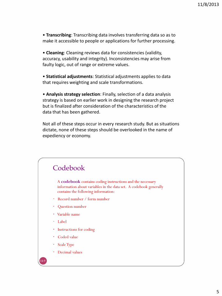
Codebook
A codebook contains coding instructions and the necessary
information about variables in the data set. A codebook generally contains the following information: Record number / form number
Question number
Variable name
Label
Instructions for coding
Coded value
Scale Type
Decimal values
14-9

11/8/2013
6
How will you code the following Situations?
10
Categorical Data Gender:
Male
[1]
Female
[2]
Your education
[1] Primary
[2] secondary
[3] Graduation
[4] Other
11

11/8/2013
7
Categorical data with multiple choices How will you code this?
Which news channel(s) do you often watch?
[
] Geo
[
] Sama
[
] Express
[
] Dunya
[
] PTV
This is not one variable, these are five variables. Each choice will be treated as one variable. Hence we will enter ‘1’ if the choice is selected or ‘0’ if the choice is not selected.
12
Continuous Rating Scale Respondents rate the objects by placing a mark at the appropriate position
on a line that runs from one extreme of the criterion variable to the other.
The form of the continuous scale may vary considerably.
How would you rate Sears as a department store?
Version 1
Probably the worst - - - - - - -I - - - - - - - - - - - - - - - - - - - - - - Probably the best
Version 2
Probably the worst - - - - - - -I - - - - - - - - - - - - - - - - - - - - - ----------------------------Probably the best
0
10
20
30
40
50
60
70
80
90
100
Version 3 Very bad
Neither good
Very good nor bad
Probably the worst - - - - - - -I - - - - - - - - - - - - - - - - - - - - ---------------------------Probably the best 0
10
20
30
40
50
60
70
80
90
100

11/8/2013
8
Likert and Other Scales The quality of the service is satisfactory:
[1] Strongly Agree
[2] Agree
[3] Neutral
[4] Disagree
[5] Strongly Disagree
[-2] Strongly Agree
[-1] Agree
[0] Neutral
[1] Disagree
[2] Strongly Disagree
Reversing the scale:
In some cases the statement has negative (opposite) meaning as
compared to the group of other statements. In that case either coding
is reversed either at the time of entry or at the time of analysis.
The quality of the service is NOT satisfactory:
[1] Strongly Agree
[2] Agree
[3] Neutral
[4] Disagree
[5] Strongly Disagree
[5] Strongly Agree
[4] Agree
[3] Neutral
[2] Disagree
[1] Strongly Disagree
14
Semantic differential scale The quality of food in this restaurant is:
Best
Worst
+3
+2
+1
0
-1
-2
-3
15

11/8/2013
9
Grid Choices Please tick ( ) or cross ( ) if you are satisfied or not satisfied in the following case.
KFC
McDonald
Pizza Hut
Service
Quality of
food
Ambiance
Price
16
Grid Choices Please write down 1 - 5 according to your level of
satisfaction in the following case.
1 = very dissatisfied, 2 = dissatisfied, 3= neutral, 4 = satisfied, 5 = very satisfied
KFC
McDonald
Pizza Hut Service
Quality of
food
Ambiance
Price
17
11/8/2013
10
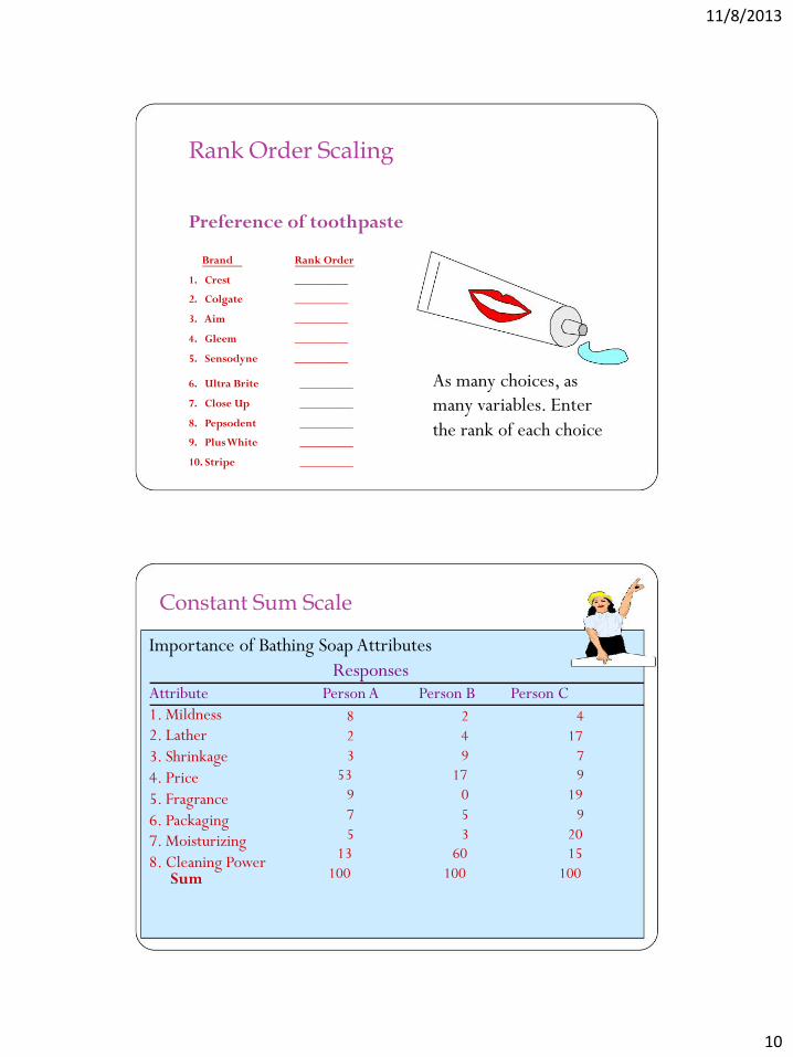
Rank Order Scaling
Preference of toothpaste
Brand Rank Order
1. Crest _________
2. Colgate _________
3. Aim _________
4. Gleem _________
5. Sensodyne _________
6. Ultra Brite _________
7. Close Up _________
8. Pepsodent _________
9. Plus White _________
10. Stripe _________
As many choices, as
many variables. Enter
the rank of each choice
Constant Sum Scale
Importance of Bathing Soap Attributes
Responses
Attribute
1. Mildness
2. Lather
3. Shrinkage
4. Price
5. Fragrance
6. Packaging
7. Moisturizing
8. Cleaning Power
Sum
Person A Person B Person C
8 2 4
2 4 17
3 9 7
53 17 9
9 0 19
7 5 9
5 3 20
13 60 15
100 100 100

11/8/2013
11
Data Cleaning & Consistency Checks
Consistency checks identify data that are out of range, logically
inconsistent, or have extreme values.
Computer packages like SPSS, SAS, EXCEL and MINITAB can
be programmed to identify out-of-range values for each variable
and print out the respondent code, variable code, variable
name, record number, column number, and out-of-range value.
Extreme values should be closely examined.
20
Data Cleaning & Treatment of Missing Responses
Substitute a Neutral Value - A neutral value, typically the mean
response to the variable, is substituted for the missing responses.
Substitute an Imputed Response - The respondents' pattern of
responses to other questions are used to impute or calculate a suitable
response to the missing questions.
In casewise deletion, cases, or respondents, with any missing
responses are discarded from the analysis.
In pairwise deletion, instead of discarding all cases with any missing
values, the researcher uses only the cases or respondents with complete
responses for each calculation.
21

11/8/2013
12
Statistically Adjusting the Data Weighting
In weighting, each case or respondent in the database is
assigned a weight to reflect its importance relative to other cases
or respondents.
Weighting is most widely used to make the sample data more
representative of a target population on specific characteristics.
Yet another use of weighting is to adjust the sample so that
greater importance is attached to respondents with certain
characteristics.
22
Statistically Adjusting the Data Use of Weighting for Representativeness
Years of
Sample
Population
Education
Percentage
Percentage
Weight
Elementary School
0 to 7 years
2.49
4.23
1.70
8 years
1.26
2.19
1.74
High School
1 to 3 years
6.39
8.65
1.35
4 years
25.39
29.24
1.15
College
1 to 3 years
22.33
29.42
1.32
4 years
15.02
12.01
0.80
5 to 6 years
14.94
7.36
0.49
7 years or more
12.18
6.90
0.57
Totals
100.00
100.00
23

11/8/2013
13
Statistically Adjusting the Data - Variable Re-specification
Variable respecification involves the transformation of data to
create new variables or modify existing variables.
For example the researcher may create new variables that are
composites of several other variables.
Dummy variables are used for respecifying categorical variables.
The general rule is that to respecify a categorical variable with K
categories, K-1 dummy variables are needed.
24
Statistically Adjusting the Data - Variable Re-specification
Product Usage
Original
Dummy Variable Code Category
Variable Code
X1
X2
X3
Nonusers
1
1
0
0 Light users
2
0
1
0 Medium users
3
0
0
1 Heavy users
4
0
0
0
Note that X1 = 1 for nonusers and 0 for all others. Likewise, X2 = 1 for light
users and 0 for all others, and X3 = 1 for medium users and 0 for all others. In
analyzing the data, X1, X2, and X3 are used to represent all user/nonuser groups.
25

11/8/2013
14
Basic Analysis
30
Internet Usage Data Respondent
Sex Familiarity
Internet
Attitude Toward
Usage of Internet
Number
Usage
Internet
Technology Shopping
Banking
1
1.00
7.00
14.00
7.00
6.00
1.00
1.00
2
2.00
2.00
2.00
3.00
3.00
2.00
2.00
3
2.00
3.00
3.00
4.00
3.00
1.00
2.00
4
2.00
3.00
3.00
7.00
5.00
1.00
2.00
5
1.00
7.00
13.00
7.00
7.00
1.00
1.00
6
2.00
4.00
6.00
5.00
4.00
1.00
2.00
7
2.00
2.00
2.00
4.00
5.00
2.00
2.00
8
2.00
3.00
6.00
5.00
4.00
2.00
2.00
9
2.00
3.00
6.00
6.00
4.00
1.00
2.00
10
1.00
9.00
15.00
7.00
6.00
1.00
2.00
11
2.00
4.00
3.00
4.00
3.00
2.00
2.00
12
2.00
5.00
4.00
6.00
4.00
2.00
2.00
13
1.00
6.00
9.00
6.00
5.00
2.00
1.00
14
1.00
6.00
8.00
3.00
2.00
2.00
2.00
15
1.00
6.00
5.00
5.00
4.00
1.00
2.00
16
2.00
4.00
3.00
4.00
3.00
2.00
2.00
17
1.00
6.00
9.00
5.00
3.00
1.00
1.00
18
1.00
4.00
4.00
5.00
4.00
1.00
2.00
19
1.00
7.00
14.00
6.00
6.00
1.00
1.00
20
2.00
6.00
6.00
6.00
4.00
2.00
2.00
21
1.00
6.00
9.00
4.00
2.00
2.00
2.00
22
1.00
5.00
5.00
5.00
4.00
2.00
1.00
23
2.00
3.00
2.00
4.00
2.00
2.00
2.00
24
1.00
7.00
15.00
6.00
6.00
1.00
1.00
25
2.00
6.00
6.00
5.00
3.00
1.00
2.00
26
1.00
6.00
13.00
6.00
6.00
1.00
1.00
27
2.00
5.00
4.00
5.00
5.00
1.00
1.00
28
2.00
4.00
2.00
3.00
2.00
2.00
2.00
29
1.00
4.00
4.00
5.00
3.00
1.00
2.00
30
1.00
3.00
3.00
7.00
5.00
1.00
2.00

11/8/2013
15
Frequency Distribution
In a frequency distribution, one variable is considered
at a time.
A frequency distribution for a variable produces a table of
frequency counts, percentages, and cumulative
percentages for all the values associated with that variable.
Frequency Distribution of Familiarity with the Internet
Valid
Cumulative
Value label
Value
Frequency (N)
Percentage percentage percentage
Not so familiar
1
0
0.0
0.0
0.0
2
2
6.7
6.9
6.9
3
6
20.0
20.7
27.6
4
6
20.0
20.7
48.3
5
3
10.0
10.3
58.6
6
8
26.7
27.6
86.2
Very familiar
7
4
13.3
13.8
100.0
Missing
9
1
3.3
TOTAL
30
100.0
100.0

11/8/2013
16
Frequency Histogram
8
7
6
5
4
3
2
1
0
2
3
4
5
6
7
Familiarity
Cross-Tabulation
While a frequency distribution describes one variable at a time, a
cross-tabulation describes two or more variables simultaneously.
Cross-tabulation results in tables that reflect the joint distribution of
two or more variables with a limited number of categories or distinct
values

11/8/2013
17
Gender and Internet Usage Gender
Row
Internet Usage
Male
Female
Total
Light (1)
5
10
15
Heavy (2)
10
5
15
Column Total
15
15
Two Variables Cross-Tabulation
Since two variables have been cross-classified, percentages could
be computed either columnwise, based on column totals or
rowwise, based on row totals
The general rule is to compute the percentages in the direction of
the independent variable, across the dependent variable. The
correct way of calculating percentages is as shown in this table.

11/8/2013
18
Internet Usage by Gender
Gender
Internet Usage
Male
Female
Light
33.3%
66.7%
Heavy
66.7%
33.3%
Column total
100%
100%
Gender by Internet Usage
Internet Usage
Gender
Light
Heavy
Total
Male
33.3%
66.7%
100.0%
Female
66.7%
33.3%
100.0%

11/8/2013
19
Purchase of Fashion Clothing by
Marital Status
Purchase of
Current Marital Status
Fashion Clothing
Married
Unmarried
High
31%
52%
Low
69%
48%
Column
100%
100%
Number of
700
300 respondents
Purchase of Fashion Clothing by
Marital Status
Purchase of
Sex Fashion
Male
Female Clothing
Married
Not
Married
Not Married
Married
High
35%
40%
25%
60%
Low
65%
60%
75%
40%
Column
100%
100%
100%
100% totals
Number of
400
120
300
180 cases

11/8/2013
20
Three Variables Cross-Tabulation Initial Relationship was Spurious Table shows that 32% of those with college degrees own an expensive automobile, as compared to 21% of those without college degrees. Realizing that income may also be a factor, the researcher decided to
reexamine the relationship between education and ownership of expensive automobiles in light of income level. In Table the percentages of those with and without college degrees who
own expensive automobiles are the same for each of the income groups. When the data for the high income and low income groups are examined separately, the association between education and ownership of expensive automobiles disappears, indicating that the initial relationship
observed between these two variables was spurious.
Ownership of Expensive Automobiles by Education Level
Own Expensive
Education
Automobile
College Degree
No College Degree
Yes
32%
21%
No
68%
79%
Column totals
100%
100%
Number of cases
250
750

11/8/2013
21
Ownership of Expensive Automobiles by Education Level and Income Levels
Income
Own
Low Income
High Income Expensive
Automobile College
No
College
No College Degree
College
Degree
Degree Degree
Yes
20%
20%
40%
40%
No
80%
80%
60%
60%
Column totals
100%
100%
100%
100%
Number of
100
700
150
50 respondents
Three Variables Cross-Tabulation Reveal Suppressed Association Table shows no association between desire to travel abroad and age.
When sex was introduced as the third variable, Table 15.11 was obtained. Among
men, 60% of those under 45 indicated a desire to travel abroad, as compared to
40% of those 45 or older. The pattern was reversed for women, where 35% of
those under 45 indicated a desire to travel abroad as opposed to 65% of those 45
or older.
Since the association between desire to travel abroad and age runs in the opposite
direction for males and females, the relationship between these two variables is
masked when the data are aggregated across sex as in Table.
But when the effect of sex is controlled, as in Table the suppressed association
between desire to travel abroad and age is revealed for the separate categories of
males and females.

11/8/2013
22
Desire to Travel Abroad by Age
Desire to Travel Abroad
Age
Less than 45
45 or More
Yes
50%
50%
No
50%
50%
Column totals
100%
100%
Number of respondents
500
500
Desire to Travel Abroad by Age and Gender
Desire to
Sex Travel
Male
Female Abroad
Age
Age
< 45
>=45
<45
>=45
Yes
60%
40%
35%
65%
No
40%
60%
65%
35%
Column
100%
100%
100%
100% totals
Number of
300
300
200
200 Cases

11/8/2013
23
Three Variables Cross-Tabulations No Change in Initial Relationship
Consider the cross-tabulation of family size and the tendency to eat
out frequently in fast-food restaurants as shown in table. No
association is observed.
When income was introduced as a third variable in the analysis,
Table was obtained. Again, no association was observed.
Eating Frequently in Fast-Food Restaurants by Family Size
Eat Frequently in Fast-
Family Size Food Restaurants
Small
Large
Yes
65%
65%
No
35%
35%
Column totals
100%
100%
Number of cases
500
500

11/8/2013
24
Eating Frequently in Fast Food-Restaurants by Family Size and Income
Income
Eat Frequently in Fast-
Low
High
Food Restaurants
Family size
Family size
Small
Large
Small
Large
Yes
65%
65%
65%
65%
No
35%
35%
35%
35%
Column totals
100%
100%
100%
100%
Number of respondents
250
250
250
250
54