quantitative analysis for business decisions - school of computing
TRANSCRIPT

CA200 – Quantitative Analysis for Business Decisions
File name: CA200_Section_04A_StatisticsIntroduction
CA200 - Quantitative Analysis for Business Decisions
CA200_Section_04A_StatisticsIntroduction Page 2 of 16
Table of Contents
4. Introduction to Statistics ............................................................................................ 1
4.1 Overview .............................................................................................................. 3
4.2 Discrete or continuous data :Variable types ........................................................ 4
4.3 Frequency distributions:Probability (Statistical) Distributions and depiction ..... 6
4.4 Characterising distributions (average, dispersion etc) ......................................... 7
4.5 Standard Continuous Distributions: (pdfs) (Normal & its tables) ..................... 12
4.6 Standard Discrete Distributions ......................................................................... 13
4.7 Exercises ............................................................................................................ 16
CA200 - Quantitative Analysis for Business Decisions
CA200_Section_04A_StatisticsIntroduction Page 3 of 16
4. Introduction to Statistics
4.1 Overview
Statistics deal with the management and quantitative analysis of data of different
types, much of it numerical. Underpinning statistical theory are the mathematics of
probability; in other words, it is possible to talk about expected outcomes and how
reliable these outcomes are, whether reproducible and so on.
Of interest, typically, in a statistical investigation, is
(i) The collection of data from past records, from targeted surveys, from
experiment and so on. Experiments can be ‘controlled’ to some extent,
whereas surveys are passive, although ’leading questions’ may be inserted
to try to obtain desired answers, which is not helful to the objectivity of
the investigation, but may help the marketing!
(ii) The analysis and interpretation of the data collected: - using a range of
statistical techniques
(iii)Use of the results, together with probabilities, costs and revenues to make
informed decisions.
Note: Much statistical data relies on sampling, as we can rarely obtain
information from (or on) every unit of the target population, (whatever that may
be). If the population is sampled correctly – i.e. using random sampling (or one of
the other variant probabilistic sampling methods), then probability rules apply and
we can use these for interpretation – as above. In effect, the correctly-drawn
sample is considered to be representative of the target population and can be
used to make estimates of different features of that population.
A sample, taken without this type of rigour – e.g. a ‘judgement’ , ‘chunk’, ‘quota’
sample, or similarly, is not a probabilistic sample and can be analysed as
descriptive of itself only and not taken to be representative of the larger group.
Starting points:
- Nature or type of data
- Grouping the data in some useful way.
2
CA200 - Quantitative Analysis for Business Decisions
CA200_Section_04A_StatisticsIntroduction Page 4 of 16
4.2 Discrete or Continuous data: Variable types
Discrete Data: has distinct values, no intermediate points, so e.g. can have values,
such as 0,1,2,3, , but not values, such as 1.5, 2.7, 4.35,…..
Continuous Data: consists of any values over a range, so either a whole number or a
fraction, so e.g. weights 10.68Kg., 14.753kg., 16kg., 21.005kg.
Random variable (i.e. a variable which can take any chance value appropriate to the
data type) is used to refer to values of the data for the measure of interest, so if X =
Discrete Random Variable = No. of Days (say), X might have values 0,1,2,3,…. If Y
= Continuous Random Variable = Distance in Miles (say), then is has a set of any
values, e.g. 12.5, 30.02, 17.8, 20.96 etc.
These random variables thus have a set of values for any given situation, which is
determined by the actual dataset that is being considered. In consequence, we can
refer to the probability of the random variable having a given value (or range of
values), and we can obtain its expected value and so on. Thus:
Discrete Distribution: discrete data generate a discrete frequency distribution (or
more generally, a description of possible outcomes by a discrete probability
distribution)
Continuous Distribution: as above, but for continuous data over an interval
(continuous range of possible measures/outcomes).
Note1: Usually, continuous distributions are more amenable to statistical analysis.
Further, where samples are large, it is often possible to assume continuity of
values, even if data type is strictly discrete.
Comment: In talking about data type and nature of measurement, we should also
recall how scales (or levels) of measurement can differ and what we can do with data
of discrete and continuous types, depending on what is being measured.
SoM / LoM include Nominal, Ordinal, Interval and Ratio
Examples
CA200 - Quantitative Analysis for Business Decisions
CA200_Section_04A_StatisticsIntroduction Page 5 of 16
Nominal -use convenient labels to differentiate categories, so e.g. M and F; e.g.
holiday types, e.g. product brands etc.
Ordinal – rank has some meaning for the data, so e.g. scale of satisfaction – very
dissatisfied, dissatisfied, find acceptable, satisfied, very satisfied. These might be
given scores 1 to 5, but these are not measurable in a numerical sense. They give rank,
but do not tell us if very satisfied is twice as happy as satisfied, for example.
(We can construct a distribution for these levels of measurement, but labelling M = 1
and F = 2 for convenience, does not give the value 1.5 a real meaning. Similarly,
subtracting dissatisfied (=2) from very satisfied (= 5), does not mean that these are
equivalent to a distance of ‘find acceptable’ apart. Merely the ranking tells us the
direction of increasing/decreasing satisfaction in relation to each other. ).
Interval : - scale is quantitative, so have equality of units, and differences and
amounts have meaning. Zero is just another point on the scale so values above and
below this are acceptable. For example, if we consider journey distance from given
start point. A is 20 miles East from starting point, B 30 miles West, so labelling the
start point zero, B as -30 and A as +20 means that A and B are 50 miles apart, A is 2/3
distance B away from start point and similarly. Another classic example is the
Fahrenheit temperature scale, which includes both negative and positive values, but
where for C and D the same no. of units apart as E and F, the same difference in
temperature in degrees Fahrenheit applies.
Ratio : the ratio scale is also a quantitative scale and has equality of units. However,
absolute zero is a defined number, so no negative values possible. Examples include
physical measures, such as volume, height, weight, age etc.
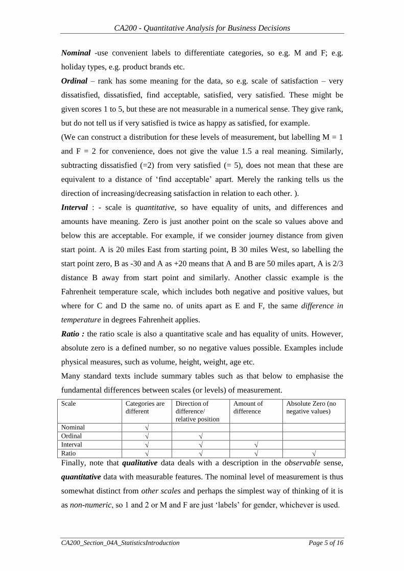
Many standard texts include summary tables such as that below to emphasise the
fundamental differences between scales (or levels) of measurement.
Scale Categories are
different
Direction of
difference/
relative position
Amount of
difference
Absolute Zero (no
negative values)
Nominal
Ordinal
Interval
Ratio
Finally, note that qualitative data deals with a description in the observable sense,
quantitative data with measurable features. The nominal level of measurement is thus
somewhat distinct from other scales and perhaps the simplest way of thinking of it is
as non-numeric, so 1 and 2 or M and F are just ‘labels’ for gender, whichever is used.
CA200 - Quantitative Analysis for Business Decisions
CA200_Section_04A_StatisticsIntroduction Page 6 of 16
4.3 Frequency distributions: Statistical Distributions – depiction
Frequency Distribution or (Relative Frequency)or (%Frequency) records actual data
values available for a given data set.
Probability Distributions (also called Statistical Distributions) describe ‘possible’
data sets, sampled data , e.g. past experience information. So, samples drawn from a
larger group or population have associated probabilities of how these might look.
Note: Also recall that a basic definitions of (objective) probability is the long-run
proportion or relative frequency, e.g. large no. coin tosees, picking a card etc.
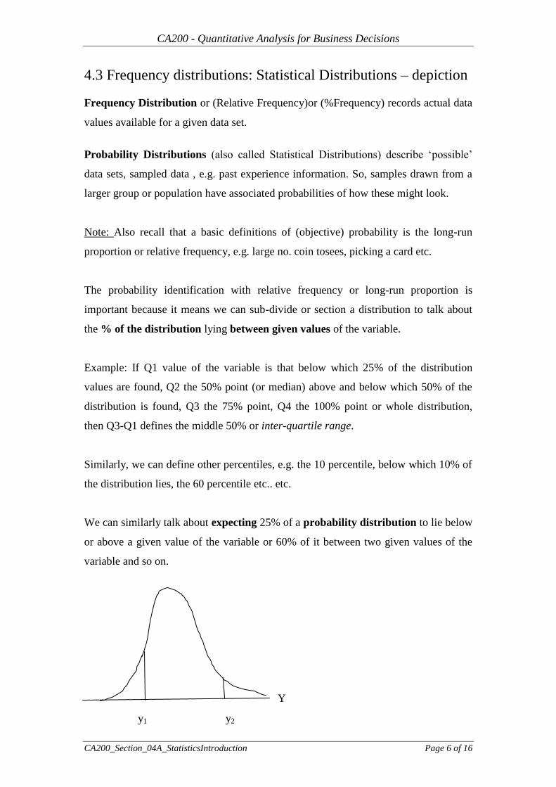
The probability identification with relative frequency or long-run proportion is
important because it means we can sub-divide or section a distribution to talk about
the % of the distribution lying between given values of the variable.
Example: If Q1 value of the variable is that below which 25% of the distribution
values are found, Q2 the 50% point (or median) above and below which 50% of the
distribution is found, Q3 the 75% point, Q4 the 100% point or whole distribution,
then Q3-Q1 defines the middle 50% or inter-quartile range.
Similarly, we can define other percentiles, e.g. the 10 percentile, below which 10% of
the distribution lies, the 60 percentile etc.. etc.
We can similarly talk about expecting 25% of a probability distribution to lie below
or above a given value of the variable or 60% of it between two given values of the
variable and so on.
Y
y2 y1
CA200 - Quantitative Analysis for Business Decisions
CA200_Section_04A_StatisticsIntroduction Page 7 of 16
4.4 Characterising Distributions: (average, dispersion etc.)
Summary Statistics: Values summarising main features of the data. These are
usually representative in some way, i.e. measures of location or central tendency or
of spread (dispersion or variability)
Random Value: could pick any one in a set of data S= {x1, x2,…. xn} , say xk.
Straightforward, but obviously extreme values can occur and successive values might
be very different.
Average:
Commonly use the Arithmetic Mean, so for set of values, S above
or for data that are grouped, where x1 occurs f1 times, x2 occurs f2 times etc.
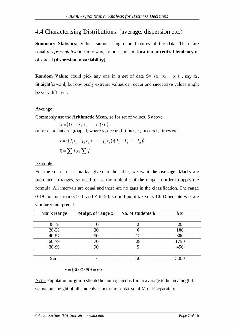
Example.
For the set of class marks, given in the table, we want the average. Marks are
presented in ranges, so need to use the midpoint of the range in order to apply the
formula. All intervals are equal and there are no gaps in the classification. The range
0-19 contains marks > 0 and to 20, so mid-point taken as 10. Other intervals are
similarly interpreted.
Mark Range Midpt. of range xi No. of students fi fi xi
0-19 10 2 20
20-38 30 6 180
40-57 50 12 600
60-79 70 25 1750
80-99 90 5 450
Sum - 50 3000
Note: Population or group should be homogeneous for an average to be meaningful,
so average height of all students is not representative of M or F separately.
nxxxx n /)....( 21
)..../()....( 212211 nnn fffxfxfxfx
fxfx /
60}50/3000{ x

CA200 - Quantitative Analysis for Business Decisions
CA200_Section_04A_StatisticsIntroduction Page 8 of 16
The Mode is another common ‘average’ measure and is that value which occurs most
frequently in the distribution of values.
The Median is the middle point of the distribution,. So, if {x1, x2, ….xn} are the
marks of the students, placed in increasing order, the median is the mark of the
(n+1)/2 th student. This is often calculated from the cumulative frequency
distribution.
For example, the median is the mark of the 25th
/ 26th
students. From the table, this is
the mark of the 5.5 th student in the 60-79 mark range, which contains 25 students and
spans 20 marks so Median = 60 + [(5.5)/25] 20 = 64.4 marks. From the diagram, it is
the 50% point in the cumulative frequency diagram of marks 0 (the more than
cumulative frequency) or 100, (the less than cumulative frequency).
Similar concepts apply for continuous distributions. The distribution function or
cumulative distribution function is defined by:
Its derivative is the frequency distribution or frequency function (or prob. density fn.)
i.e.
x 20 40 60 80 100
50
}{)( xXPxF
dxxdfxf )()(
dxxfxF )()(

CA200 - Quantitative Analysis for Business Decisions
CA200_Section_04A_StatisticsIntroduction Page 9 of 16
Dispersion or Spread
An ‘average’ alone may not be adequate, as distributions may have the same
arithmetic mean, but the values may be grouped very differently. For a distribution
with small variability or dispersion, the distribution is concentrated about the mean.
For large variability, the distribution may be very scattered.
The average of the squared deviations about the mean is called the variance and
this is the commonly used statistical measure of dispersion. The square root of the
variance is called the standard deviation and has the same units of measurement as
the original values.
To illustrate why the variance is needed, consider a second set of student marks and
compare with the first. Both have the same mean, but the variability of the second set
is much higher, i.e. marks are much more dispersed or scattered about the mean value.
Example:
First Set of Marks Second Set of Marks
f x fx fx2
f x fx fx2
2 10 20 200 6 10 60 600
6 30 180 5400 8 30 240 7200
12 50 600 30000 6 50 300 15000
25 70 1750 122500 15 70 1050 73500
5 90 450 40500 15 90 1350 121500
50 3000 198600 50 3000 217800
Then for set 1:
Var(x) =198600/50 – (60)2
= 372 marks2 i.e. s.d. = 19.3 marks
for set 2:
Var(x) = 217800/50 – (60)2 = 756 marks
2 i.e. s.d. = 27.5 marks
)(.. xVarDS
fdeviationssquaredfxVar /)(2
2
22
2
)()(
)( xf
xf
f
xxf
xVar i
i
i
i

CA200 - Quantitative Analysis for Business Decisions
CA200_Section_04A_StatisticsIntroduction Page 10 of 16
Other Summary Statistics, characterising distributions
Average Measures (other than Arithmetic Mean): there are a number of these, apart
from the simple ones of the mode and median.
Other Dispersion Measures
Range = Max. value – Min. value
Inter-quartile Range = Q3 –Q1 (as before)
Skewness
Degree of symmetry. Distributions that have a large tail of outlying values on the
right-hand-side are called positively skewed or skewed to the right. Negative
skewness refers to distributions with large left-hand tail.
A simple formula for skewness is
Skewness = ( Mean - Mode ) / Standard Deviation
so, for Set 1 of student marks:
Skewness = (60 - 67.8) / 19.287 = - 0.4044.
Kurtosis
-measures how peaked the distribution is; 3 broad types ate Leptokurtic - high peak,
mesokurtic, platykurtic – flattened peak.
Characterising Probability (Statistical) Distributions:
We have seen examples of this already in the work on expected values and decision
criteria.
Example: X = random variable = Distance in km. travelled by children to school. Past
records show probability distribution to be as below. Calculations are similar.
pi xi pixi pixi2
0.15 2.0 0.30 0.60
0.40 4.0 1.60 6.40
0.20 6.0 1.20 7.20
0.15 8.0 1.20 9.60
0.10 10.0 1.00 1.00
1.00 E(x) = = 5.30 33.80
Then Expected Value of X = E(X) = 5.30 km.
Variance of X = Var(X) = 33.80 - (5.30)2 = 5.71 km.
2

CA200 - Quantitative Analysis for Business Decisions
CA200_Section_04A_StatisticsIntroduction Page 11 of 16
Standard Probability (or Statistical) Distributions
For a summary of commonly used statistical distributions – see any statistical
textbook.
Importantly, characterised by expectation and variance (as for random variables) and
by the parameters on which these are based.
E.g.for a Binomial distribution, the parameters are p the probability of success in an
individual trial and n the No. of trials.
The probability of success remains constant – otherwise, another distribution applies.
Use of the correct distribution is core to statistical inference – i.e. estimating
population values on the basis of a (correctly drawn, probabilistic) sample.
The sample is then representative of the population- (sampling theory)

CA200 - Quantitative Analysis for Business Decisions
CA200_Section_04A_StatisticsIntroduction Page 12 of 16
4.5 Standard Continuous Distns. (pdfs): Normal (& Tables)
Fundamental to statistical inference (Section 5) is the Normal (or Gaussian), with
parameters, the mean (or more formally) expectation of the distribution) and (or
2
), the Standard deviation (Variance) respectively. A random variable X has a
Normal distribution with mean µ and standard deviation if it has density
Notes:
The Normal distribution is also the so-called ‘limiting’ distribution of the Mean of a
set of independent and identically distributed random variables: this means that if you
have a distribution of values for a random variable X, then whatever the distribution
for X looks like, the distribution of is Normal; ~ N, providing that the
sample size is sufficiently large.
This result is called the Central Limit Theorem and plays a fundamental role in
sampling theory and statistical inference, as it means that the Normal distribution can
often be used to describe values of a variable or its mean or proportion.
Further, the Normal can also be used to approximate many empirical data. Default
in much empirical work is to assume observations are distributed (~) approx. as N.
It can also be used to approximate discrete distributions if the sample size is large.
Tables:
Given that a Normal distribution can be generated for any combination of mean ()
and variance (2), this implies very many tables would be needed to be able to work
out probabilities of (say) % of a distribution between given values, unless we wished
to calculate these from first principles! Fortunately, a simple transformation means
that Standardised Normal Tables can be used for any value of the mean and standard
deviation (or variance).
X is said to be a Standardised Normal Variable, (U), if = 0 and 2 (or ) = 1.
[For Normal Tables, (i.e. Standardised Normal Tables, see pages 13 sand 14 in White,
Yeats and Skipworth, “Tables for Statisticians.” ]
otherwiseand
xforx
xf
0
21exp
21
)(
2
X X

CA200 - Quantitative Analysis for Business Decisions
CA200_Section_04A_StatisticsIntroduction Page 13 of 16
4.6 Standard Discrete Distributions
Importance
Modelling practical applications (such as counts, binary choices etc.)
Mathematical properties known
Described by few parameters, which have natural interpretations.
Bernoulli Distribution.
This is used to model a single trial or sample, which gives rise to just two outcomes:
e.g. male/ female, 0 / 1.
Let p be the probability that the outcome is one and q = 1 - p that the outcome is zero,
then have:
E[X] = p (1) + (1 - p) (0) = p
VAR[X] = p (1)2
+ (1 - p) (0)2
- E[X]2
= p (1 - p).
Binomial
Suppose that we are interested in the number of successes X in a number ‘n’ of
independent repetitions of a Bernoulli trial, where the probability of success in an
individual trial is constant and = p. Then
Prob {X = k} = n
Ck p
k
(1-p)n - k
, (k = 0, 1, …, n)
E[X] = n p
VAR[X] = n p (1 - p)
where Binomial Coefficients are the No. combinations of n items, taken k at a time.
The shape of the distribution depends on the value of n and p.
As p ½ and n increases, it becomes increasingly symmetric
(and can be approximated by the Normal for large n)
k
nwrittenalsoCk
n
0 p 1 x
1 Prob.
p
1-p
Prob. 1
0 1 2 3 4 x
np
CA200 - Quantitative Analysis for Business Decisions
CA200_Section_04A_StatisticsIntroduction Page 14 of 16
Poisson Distribution
The Poisson distribution = limiting case of the Binomial distribution, where n ∞ ,
p 0 in such a way that np , the Poisson parameter
The Poisson is used to model the No.of occurrences of a certain phenomenon in a
fixed period of time or space, e.g. people arriving in a queue in a fixed interval of
time, e.g. No. of fires in given period, See insurance example Section 3B). we can
therefore think of the Poisson as the rare event Binomial, i.e. p small. Its shape
depends on the value of p and n (i.e. value of ) ; usually right –skewed (positive-
skewed) for p small, n small,
Note:
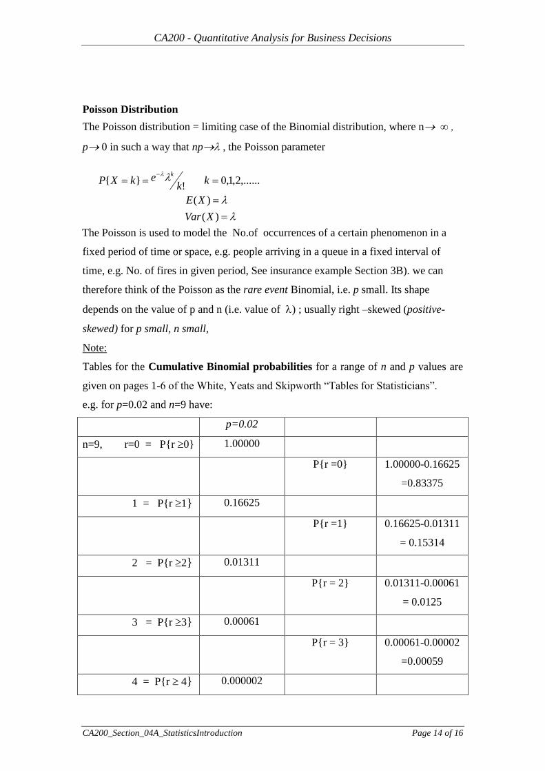
Tables for the Cumulative Binomial probabilities for a range of n and p values are
given on pages 1-6 of the White, Yeats and Skipworth “Tables for Statisticians”.
e.g. for p=0.02 and n=9 have:
p=0.02
n=9, r=0 = P{r 0} 1.00000
P{r =0} 1.00000-0.16625
=0.83375
1 = P{r 1} 0.16625
P{r =1} 0.16625-0.01311
= 0.15314
2 = P{r 2} 0.01311
P{r = 2} 0.01311-0.00061
= 0.0125
3 = P{r 3} 0.00061
P{r = 3} 0.00061-0.00002
=0.00059
4 = P{r 4} 0.000002
)(
)(
,......2,1,0!
}{
XVar
XE
kk
ekXPk
CA200 - Quantitative Analysis for Business Decisions
CA200_Section_04A_StatisticsIntroduction Page 15 of 16
Tables for the Cumulative Poisson probabilities for a range of values are given
on pages 7-10 of the White, Yeats and Skipworth “Tables for Statisticians” and
probabilities for exact values 0,1,2, etc. are calculated as for the Binomial example
above.
Example:
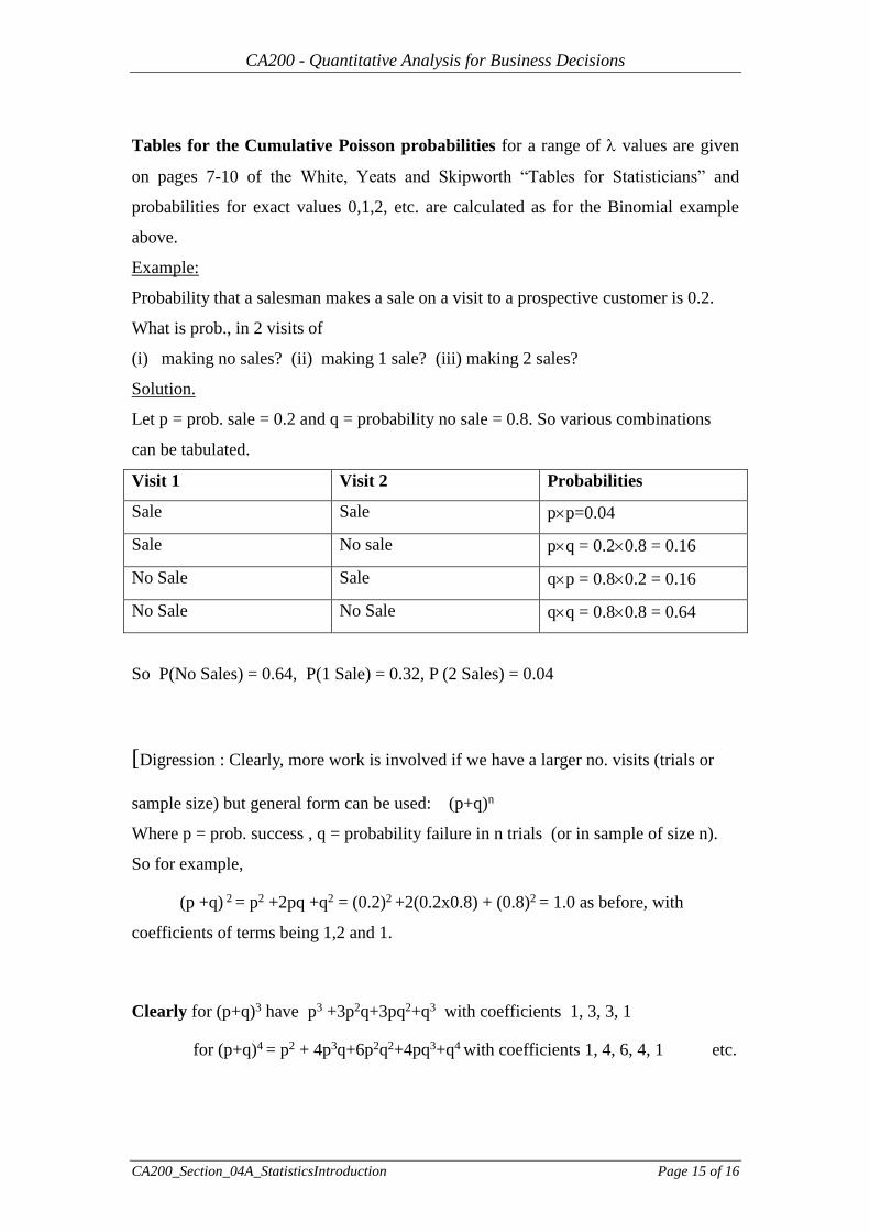
Probability that a salesman makes a sale on a visit to a prospective customer is 0.2.
What is prob., in 2 visits of
(i) making no sales? (ii) making 1 sale? (iii) making 2 sales?
Solution.
Let p = prob. sale = 0.2 and q = probability no sale = 0.8. So various combinations
can be tabulated.
Visit 1 Visit 2 Probabilities
Sale Sale pp=0.04
Sale No sale pq = 0.20.8 = 0.16
No Sale Sale qp = 0.80.2 = 0.16
No Sale No Sale qq = 0.80.8 = 0.64
So P(No Sales) = 0.64, P(1 Sale) = 0.32, P (2 Sales) = 0.04
[Digression : Clearly, more work is involved if we have a larger no. visits (trials or
sample size) but general form can be used: (p+q)n
Where p = prob. success , q = probability failure in n trials (or in sample of size n).
So for example,
(p +q) 2 = p2 +2pq +q2 = (0.2)2
+2(0.2x0.8) + (0.8)2 = 1.0 as before, with
coefficients of terms being 1,2 and 1.
Clearly for (p+q)3 have p3 +3p2q+3pq2+q3
with coefficients 1, 3, 3, 1
for (p+q)4 = p2 + 4p3q+6p2q2+4pq3+q4 with coefficients 1, 4, 6, 4, 1 etc.
CA200 - Quantitative Analysis for Business Decisions
CA200_Section_04A_StatisticsIntroduction Page 16 of 16
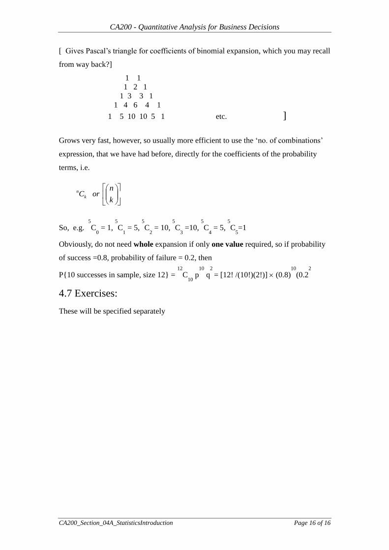
[ Gives Pascal’s triangle for coefficients of binomial expansion, which you may recall
from way back?]
1 1
1 2 1
1 3 3 1
1 4 6 4 1
1 5 10 10 5 1 etc. ]
Grows very fast, however, so usually more efficient to use the ‘no. of combinations’
expression, that we have had before, directly for the coefficients of the probability
terms, i.e.
So, e.g.
5
C0 = 1,
5
C1 = 5,
5
C2 = 10,
5
C3 =10,
5
C4 = 5,
5
C5=1
Obviously, do not need whole expansion if only one value required, so if probability
of success =0.8, probability of failure = 0.2, then
P{10 successes in sample, size 12} = 12
C10
p10
q2
= [12! /(10!)(2!)] (0.8)10
(0.22
4.7 Exercises:
These will be specified separately
k
norCk
n